the Creative Commons Attribution 4.0 License.
the Creative Commons Attribution 4.0 License.
 | 07 Dec 2023
A year of transient tracers (chlorofluorocarbon 12 and sulfur hexafluoride), noble gases (helium and neon), and tritium in the Arctic Ocean from the MOSAiC expedition (2019–2020)
Oliver Huhn
Maren Walter
Natalia Sukhikh
Salar Karam
Wiebke Körtke
Myriel Vredenborg
Klaus Bulsiewicz
Jürgen Sültenfuß
Ying-Chih Fang
Christian Mertens
Benjamin Rabe
Sandra Tippenhauer
Jacob Allerholt
Hailun He
David Kuhlmey
Ivan Kuznetsov
Maria Mallet
Trace gases have demonstrated their strength for oceanographic studies, with applications ranging from the tracking of glacial meltwater plumes to estimates of the abyssal overturning duration. Yet measurements of such passive tracers in the ice-covered Arctic Ocean are sparse. We here present a unique data set of trace gases collected during the Multidisciplinary drifting Observatory for the Study of Arctic Climate (MOSAiC) expedition, during which R/V Polarstern drifted along with the Arctic sea ice from the Laptev Sea to Fram Strait, from October 2019 to September 2020. During the expedition, trace gases from anthropogenic origin (chlorofluorocarbon 12 (CFC-12), sulfur hexafluoride (SF6), and tritium) along with noble gases (helium and neon) and their isotopes were collected at a weekly or higher temporal resolution throughout the entire water column (and occasionally in the snow) from the ship and from the ice. We describe the sampling procedures along with their challenges, the analysis methods, and the data sets, and we present case studies in the central Arctic Ocean and Fram Strait to illustrate possible usage for the data along with their robustness. Combined with simultaneous hydrographic measurements, these trace gas data sets can be used for process studies and water mass tracing throughout the Arctic in subsequent analyses. The two data sets can be downloaded via PANGAEA: https://doi.org/10.1594/PANGAEA.961729 (Huhn et al., 2023a) and https://doi.org/10.1594/PANGAEA.961738 (Huhn et al., 2023b).
- Article
(6873 KB) - Full-text XML
- BibTeX
- EndNote


The Arctic Ocean is changing rapidly in response to ongoing climate change (Meredith et al., 2019). In the upper ocean, the sea ice cover is thinning and reducing, overall (e.g. Kwok, 2018), while freshwater input from glaciers, rivers, and the atmosphere (Solomon et al., 2021) as well as heat input from the global ocean (Polyakov et al., 2020) are changing. These factors have notably resulted in contrasting changes in the stratification in the Arctic basins (Polyakov et al., 2018) and in an intensification of the Beaufort Gyre (Timmermans and Toole, 2023). As the exact processes responsible for these changes remain unclear, so does the future of the upper Arctic Ocean (Muilwijk et al., 2023). In the deeper layers of the Arctic Ocean, we do not even know whether there is a change, as hydrographic observations deeper than 1000 m are too sparse in space and time for proper dynamics studies (Heuzé et al., 2022). There is an urgent need to establish a baseline for the under-observed full-depth Arctic Ocean circulation, including its spatial and temporal variability, and to observe changes in near-real time. We argue that passive tracers, as presented in this paper, are the ideal tool to not only increase data coverage in the Arctic, but also study the processes that impact the Arctic Ocean.
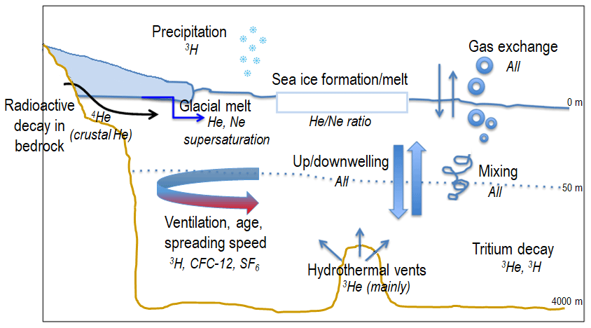
Figure 1Schematic of the ocean–ice–atmosphere interactions (plain font) affecting the tracers (italics) sampled during MOSAiC. Not included is the river runoff, relevant for 3H.
To study the full-depth ocean circulation, we need prolonged measurements over a large area at relatively high spatial and temporal resolutions. In the rest of the world ocean, thousands of autonomous profilers have been monitoring the upper 2000 m since the 1990s (Johnson et al., 2022). Although ice-avoidant and/or ice-tethered profilers have been deployed in the Arctic (Toole et al., 2011), their uninterrupted operation remains a challenge in the ice-covered ocean. Besides, they are limited to the upper 1000 m; to the best of our knowledge, no full-depth autonomous profiler has been deployed in the Arctic Ocean yet. Another option is to use trace gases, which has been done since the beginning of modern-day Arctic research (e.g. Top et al., 1983; Schlosser et al., 1990; Tanhua et al., 2009; Rajasakaren et al., 2019). The trace gases that we focus on here are all passive tracers; that is, they are not affected by chemical or biological activity. Consequently, by comparing their concentration throughout the water column or between profiles, one can infer the processes that have affected the water, the water circulation, and even the age of the water. These tracers have different sources and, therefore, different applications, which are schematically represented in Fig. 1.
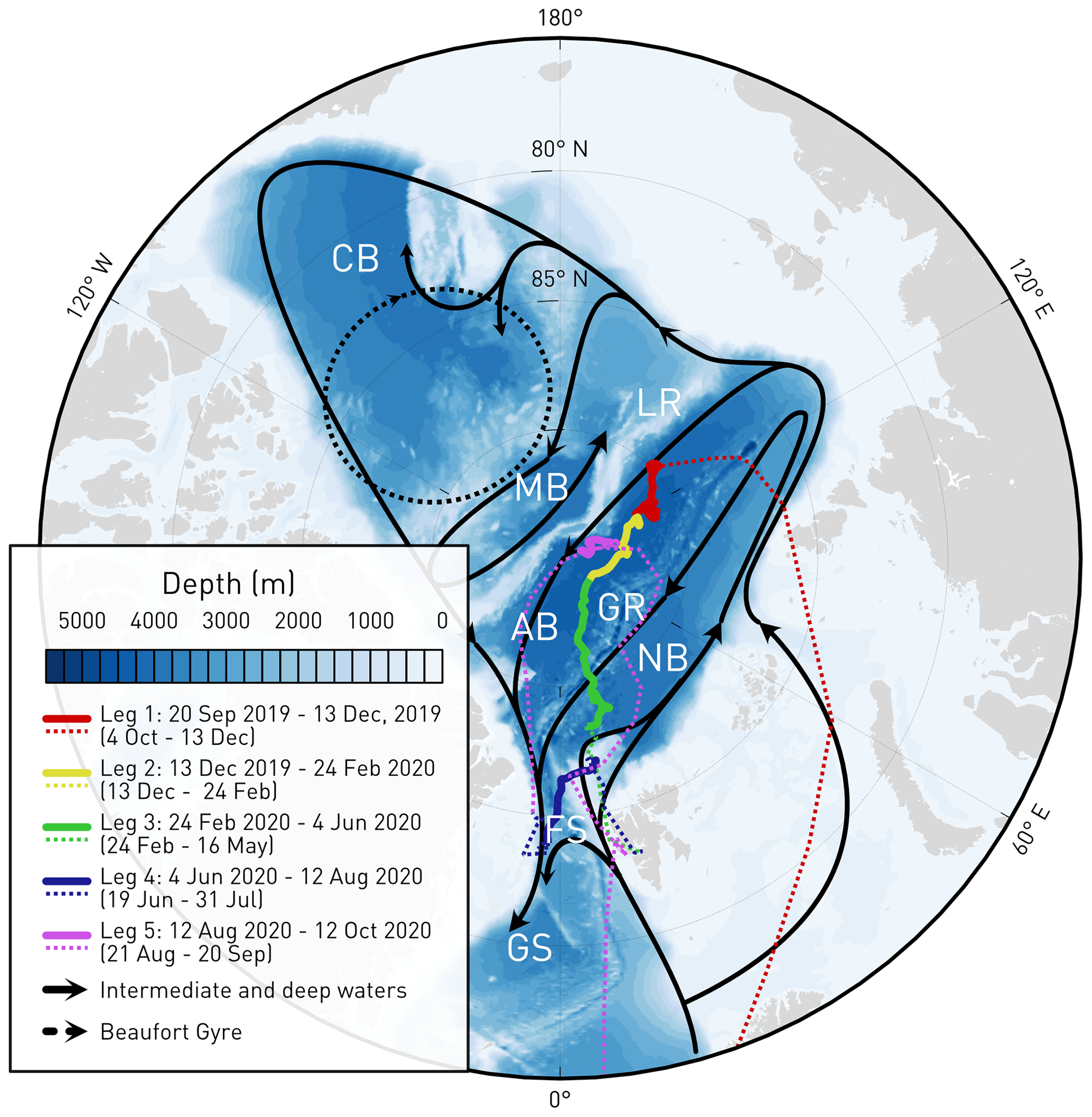
Figure 2Track of the five legs of the MOSAiC expedition. Solid lines show when R/V Polarstern was drifting with the sea ice, and dotted lines show the transit. Dates for each leg are given, with dates excluding transit in parentheses. Solid black arrows show the main circulation features of the Arctic Ocean intermediate (Atlantic) and deep waters, and the dashed black arrow shows the approximate location of the Beaufort Gyre. The place names discussed in the text are Greenland Sea (GS), Fram Strait (FS), Nansen Basin (NB), Gakkel Ridge (GR), Amundsen Basin (AB), Lomonosov Ridge (LR), Makarov Basin (MB), and Canada Basin (CB). The bathymetry (blue-to-white shading) is from the International Bathymetric Chart of the Arctic Ocean (IBCAO; Jakobsson et al., 2020), and the land mask is from A Global Self-consistent, Hierarchical, High-resolution Geography Database (GSHHG; Wessel and Smith, 1996).
The inert and stable noble gases helium (He) and neon (Ne) are abundant in the atmosphere but have a low solubility. Consequently, supersaturation at the surface indicates that processes that inject air bubbles, e.g. wave breaking or wind, have recently taken place (e.g. Hahm et al., 2004). Below the surface, excess helium and neon allow for the detection and even quantification of glacial/basal meltwater (e.g. Schlosser, 1986; Beaird et al., 2015; Huhn et al., 2021a): atmospheric air with a constant composition of these noble gases is trapped in the ice matrix during formation of the meteoric ice. Due to the enhanced hydrostatic pressure at the base of the shelf ice, these gases are completely dissolved in the water when the ice is melting from below. This leads to an excess of He of 1280 % and Ne of 890 % in pure meltwater (Loose and Jenkins, 2014). Besides, glacial meltwater can be enriched by crustal 4He, leading to anomalously high ratios in the relative vicinity of Greenland fjords (Beaird et al., 2015; Huhn et al., 2021a). In the central Arctic, the ratio at the surface is a proxy for sea ice processes as the noble gases fractionate during sea ice formation: the lighter He is incorporated into the ice matrix, whereas Ne is rejected along with the brine. Anomalously low ratios of approx. −2 % can therefore indicate recent sea ice formation (e.g. Top et al., 1983; Hahm et al., 2004).
The helium isotope 3He has its main source in the Earth's interior, the mantle and crust. This primordial helium gets injected into the deep ocean via the hydrothermal circulation of seawater through the crust, which leads to an excess in 3He compared to the atmospheric equilibrium value of the isotopic ratio found in the upper ocean. Thus, the isotopic ratio (specifically δ3He, the excess 3He compared to the atmospheric ratio) can be used as a tracer for hydrothermal venting (German et al., 2022) and the vertical exchange between the interior ocean and the upper layers (Rhein et al., 2010). The other source of excess 3He is tritiugenic, i.e. it is produced by the decay of tritium. Note that the component separation of helium, especially tritiugenic and terrigenic 3He, is complicated and requires the use of additional environmental information (Roether et al., 1998). Tritium (3H) is the radioactive isotope of hydrogen, and it enters the ocean as a result of nuclear testing in the 1960s via meteoric water from water vapour exchange, local precipitation, and continental runoff, making it an ideal tracer for studying the penetration of surface waters into the deep. Its half-life is 12.32 years, and simultaneous measurements of tritium and its decay product 3He can also be used as an age tracer. Tritium can also be a by-product of nuclear fission reactors. However emissions from European coastal plants are too diluted by the time they reach the Arctic to be detectable (Oms et al., 2019), and those from nuclear submarine normal operations have been deemed insignificant (Curren, 1988).
Chlorofluorocarbon 12 (CFC-12) and sulfur hexafluoride (SF6) are anthropogenic trace gases with well-known atmospheric concentrations (Bullister, 2015; Dutton et al., 2022a, b). The gases are well mixed in the atmosphere with only a small difference between the Northern Hemisphere and Southern Hemisphere. The atmospheric CFC concentrations increased exponentially in the 1970s, linearly afterwards, and the growth rate started to decrease after the Montreal Protocol of 1987. CFC-12 reached its peak in atmospheric concentration in 2002/03. For SF6, the increase still continues; thus, it can be used for younger, more recently ventilated, waters. For the ocean, the atmosphere is the only source of the trace gases CFC-12 and SF6, since there are no significant natural sources. The gases enter the surface waters of the ocean through air–sea gas exchange and can reach equilibrium concentration with the atmosphere (Fine, 2011). However, especially in the Arctic Ocean and for SF6, a 100 % saturation is normally not reached due to a too slow adaption to changing conditions (e.g. Smith et al., 2022; Tanhua et al., 2009).
The tracers can also be combined to shed light on specific processes, most often by first computing the transit time distribution (TTD), which is a measure of the age spectrum of a water mass (e.g. Tanhua et al., 2009). For example, Jenkins et al. (2015) used He and tritium to determine the age of the water and thus detect a signature of upwelling. Mauldin et al. (2010) used He, tritium, and CFCs together to determine the width, velocity, and mixing timescale of the Arctic Ocean Boundary Current. As these tracers also have different solubilities and equilibration times (see Appendix A1), one can compare their values to detect changes in temperature, salinity, or wind. Individually though, each tracer will be most adapted to different water mass ages, with noble gases more relevant for comparatively young waters and CFC-12 and SF6 for older ones (e.g. Waugh et al., 2003), and they will therefore often not be sampled over the same depth ranges, as was done here.
We report on trace gas measurements of CFC-12, SF6, helium, neon, and tritium made as part of the physical oceanography programme of the Multidisciplinary drifting Observatory for the Study of Arctic Climate (MOSAiC) expedition. From October 2019 to September 2020, the German icebreaker R/V Polarstern (Knust, 2017) drifted with the sea ice pack within the Eurasian Arctic (Fig. 2) and served as a scientific platform, allowing for the collection of water samples throughout the entire water column even in the middle of winter. The expedition and overall physical oceanography programme are described in detail in Rabe et al. (2022). We here describe the sampling strategy in the field in Sect. 2, while laboratory analyses are described in Sect. 3. The data sets are briefly described in Sect. 4. In Sect. 5, we demonstrate the validity of our data and show possible applications using samples from two distinct regions: the central Arctic and Fram Strait. We conclude in Sect. 7 with a brief discussion of the wider scope of the data sets and the lessons learnt from MOSAiC.
2.1 Objectives of the tracer sampling
There were two main aims for the tracer sampling during MOSAiC:
-
The first aim is to study upper ocean dynamics, including the subsurface warm and salty Atlantic Water layer (hereafter referred to as “Atlantic Water”). The goal is a better understanding of the mixed layer processes in the horizontal and vertical, with a focus on the role of the sea ice and the proximity of the ice edge, and how it affects the exchange of heat between atmosphere, mixed layer, and the heat sources in the interior (i.e. the Atlantic Water). The combination of the anthropogenic tracers (CFC-12, SF6) with the noble gas isotopes and tritium is used to study the integral effect of events like leads, eddies, and storms on the mixed layer properties and the vertical exchange between the mixed layer and the Atlantic Water.
-
The second aim is to study deep ocean dynamics also including the Atlantic Water. The goal is to determine the deep oceanic circulation in the Arctic, notably which route(s) the deep waters take, the ventilation processes, and the age of the waters. Only CFC-12 and SF6 were sampled for this; future efforts to track the ventilation should also sample tritium, while measurements above Gakkel Ridge of helium would be ideal. Other tracers could also be used, such as 14C or 39Ar, although measurements of 14C are now becoming more uncertain because of the addition of anthropogenic carbon (Koeve et al., 2015), while 39Ar still requires too large volumes (5 L, admittedly improved from its previous 1000 L) to be easily implemented on multidisciplinary, ecosystem-heavy expeditions (Ebser et al., 2018).
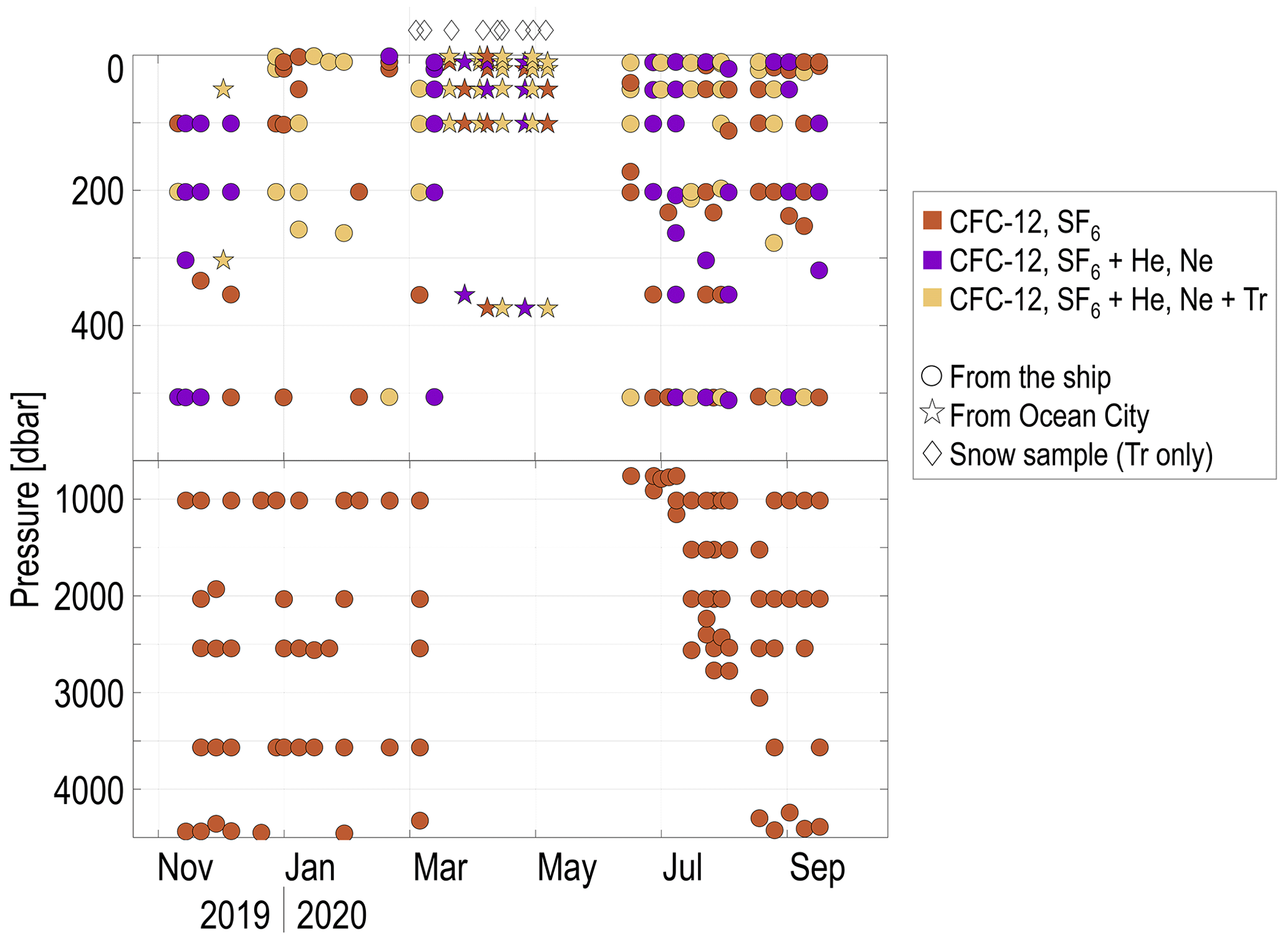
Figure 3Depth and date of all the samples included in this data set. Note the discontinued y axis. Red shows where only CFC-12/SF6 data were collected, purple where noble gases were additionally sampled, and yellow dots where tritium was sampled in addition to all other tracers. Circles indicate that the sample was collected from the ship, whereas stars denote samples from Ocean City. Diamonds above the panel indicate the dates in March to May 2020 (Leg 3) of the tritium (Tr) from snow samples.
For both the upper and deeper ocean, studies are ongoing to detangle the temporal (Fig. 3) and spatial (Fig. 4) variabilities of all these processes.
The two main aims resulted in the following general sampling strategy: during the weekly hydrographic casts (conductivity–temperature–depth or CTD) from the ship (Rabe et al., 2022), tracer samples were collected from a water bottle rosette over 12 depth levels covering the entire water column (circles in Fig. 3). Additional sampling over the upper 500 m took place from CTD casts in the ice camp (Ocean City or OC), mainly during spring (stars in Fig. 3). Trace gas samples were the first to be collected at the rosette to avoid potential degassing. Prior to sampling, the metal tubing and intake adapter were cleaned with isopropanol to remove any fat, and the person sampling made sure to not directly touch these parts. We now describe the procedure for each specific sampling.
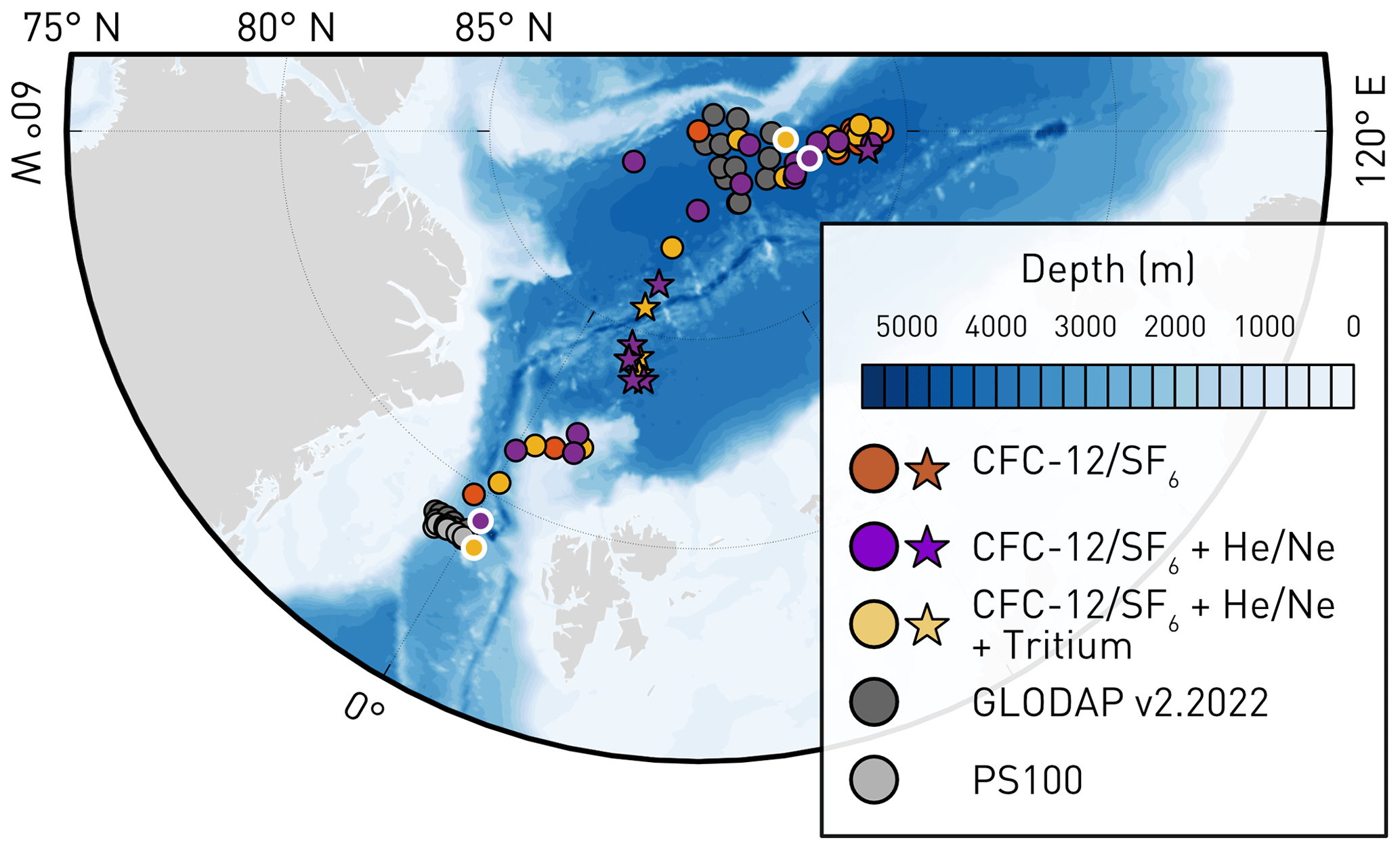
Figure 4Location of tracer data collected during the MOSAiC expedition. Red colours show where only CFC-12/SF6 data were collected, purple colours where were additionally sampled, and yellow colours where tritium was sampled in addition to all other tracers. The circles denote samples taken from the ship, whereas the stars denote samples from Ocean City. The location of the four example casts analysed in Sect. 5 are denoted by thick, white outlines, and the reference values to which they are compared are denoted with grey dots (see main text). Bathymetry (blue-to-white shading) is from IBCAO (Jakobsson et al., 2020); land mask is from GSHHG (Wessel and Smith, 1996).
2.2 Sampling of helium and neon, tritium, and CFC-12 and SF6
In total, we took 290 water samples for stable noble gas isotopes (3He, 4He, 20Ne, 22Ne) during Legs 1–5 (purple and yellow in Figs. 3 and 4). The water samples were stored from the CTD/water bottle rosettes (ship and Ocean City) without contact to atmospheric air in 40 mL gas-tight copper tubes, which are clamped off at both sides. They were collected straight after the CFC-12/SF6 samples if at the same rosette bottle, and they were collected first if no transient tracer sample was needed at that bottle. The person that was sampling took great care to rid the plastic tubing for sampling of any bubble by letting the water flow for as long as necessary and by regularly hitting the copper tube with a wrench.
For tritium measurements, we took 143 sea-water samples during Legs 1–5 (yellow in Figs. 3 and 4). The samples were stored in 500 mL plastic water bottles from the CTD/water bottle rosettes (ship and Ocean City). Additionally, we opportunistically took nine samples from snow and placed them into 2×500 mL plastic bottles during Leg 3 (diamonds in Fig. 3).
For the transient tracers CFC-12 and SF6, we took 410 samples during Legs 1–5, all the way to the sea floor (red, purple, and yellow in Figs. 3 and 4). The CFC-12 and SF6 water samples from the CTD/water bottle systems were stored in 220 mL glass ampoules, avoiding contact with the atmosphere during the tapping by a dedicated tubing and rinsing procedure. After sampling, the ampoules were flame sealed after a headspace of pure nitrogen had been applied. Flame-sealing started immediately after the sampling, but due to the large number of samples and the fact that only one sample could be sealed at a time, up to 6 h passed between sampling and the sealing of the last ampoule.
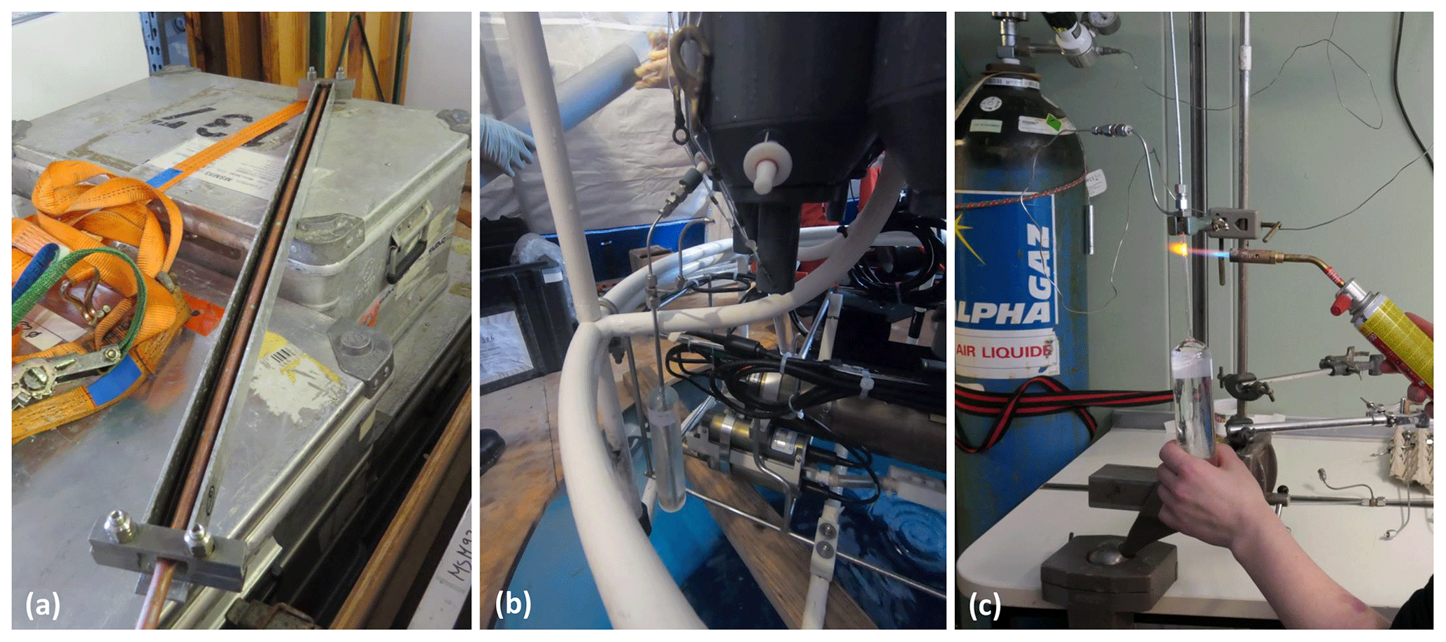
Figure 5Photos illustrating sampling challenges: (a) 90 cm long rigid copper tube for noble gas sampling (credit: Wiebke Körtke); (b) sampling of CFC-12 and SF6 during Leg 3 from Ocean City (tent on the sea ice) with the deep ocean directly below our ampoules (credit: Natalia Sukhikh); (c) flame sealing of the CFC-12 sample on board R/V Polarstern (credit: Janin Schaffer).
The sampling strategy had to be adapted during Leg 3 due to the loss of the ship-CTD hydrohole by compressed ice (Rabe et al., 2022). Combined with the uncertainties from the development of Covid-19, it was decided that the ship would not be moved to open a new hole. It was therefore impossible to sample from the ship and perform deep water sampling from March to May, when the ship eventually moved to exchange personnel. Consequently, key regions of interest such as the Amundsen–Nansen basin transition and the Gakkel Ridge were not covered with deep samples (stars in Figs. 3 and 4).
Noble gas samples and flame-sealed transient tracer samples were stored on board the ship until the end of the expedition. They were then analysed at the Institute of Environmental Physics (IUP) of the University of Bremen, Germany, following standard procedures (Bulsiewicz et al., 1998; Sültenfuß et al., 2009), as described in the following subsections.
3.1 Helium and neon samples
In the IUP Bremen noble gas lab, the samples were pre-processed with a UHV (ultra-high-vacuum) gas extraction system. Sample gases are transferred via water vapour into a glass ampoule kept at liquid nitrogen temperature. For analysis of the noble gas isotopes, the glass ampoules were connected to a fully automated UHV mass spectrometric system equipped with a two-stage cryogenic system, a quadrupole, and a sector-field mass spectrometer. Regularly, the system is calibrated with atmospheric air standards (reproducibility <0.2 %). Measurement of line blanks and linearity are done as well. The performance of the Bremen facility is described in Sültenfuß et al. (2009).
Noble gas concentrations are reported in nanomole per kilogram (nmol kg−1, for total He = 4He + 3He and total Ne = 20Ne + 22Ne) or percent (for 3He) such as
However, for presentation in this paper, we use for total He and total Ne the gas excess in percent:
using the equilibrium functions Heequilibrium= f(T,S) and Neequilibrium= f(T,S) from Weiss (1971), where T and S are the potential temperature and practical salinity as recorded at the Niskin bottle. The advantage of this common unit for noble gases is that it removes the equilibrium concentration caused by atmospheric gas exchange for the given T and S and shows only the gas-excess caused by, for example, bubble injection, basal glacial meltwater, hydrothermal addition, or other processes inside the ocean. Ultimately, 208 samples were analysed successfully, including 25 pairs of replicate samples that were each averaged for the final data set. The precision is 0.4 % for He, 0.7 % for Ne, and 0.8 % for δ3He (based on the 25 pairs of replicate measurements). Twenty-two samples were flagged doubtful; these error flags are based on a comparison with other properties and identification as outliers.
3.2 Tritium samples
In the IUP Bremen noble gas lab, the water samples were pre-processed with a gas extraction system for complete degassing and were then stored for several months. During that time, part of the tritium (3H) decayed by beta decay to helium-3 (3He). The newly produced 3He was then analysed by the same mass spectrometer system as described above. Tritium concentrations reported here are scaled to 1 January 2020 and referred to as TU-2020. Concentrations are given in TU (tritium unit), where 1 TU is the ratio of 1 tritium atom to 1018 hydrogen atoms. Typical errors for this data set are 0.04 TU or 3 %, whichever is largest.
3.3 CFC-12 and SF6 samples
The determination of CFC-12 and SF6 concentrations in the IUP Bremen gas chromatography lab was accomplished by purge and trap (cryogenic trapping at −65 ∘C) sample pre-treatment of a precise water volume of 140 mL followed by gas chromatographic separation on a capillary column and electron capture detection (ECD). After thermal desorption, the released gases are separated on a pre-column of type Aluminia Bond/CFC (0.54 mm ID × 3 m) and a main column of type Aluminia Bond/CFC (0.54 mm ID × 30 m). SF6 and CFC-12 are then detected on a micro-ECD.
The analytical system is calibrated frequently by analysing different volumes of known standard gas concentrations. The loss of CFC-12 and SF6 into the headspace is considered by equilibration between liquid and gas phases under controlled conditions before the sealed ampoules are opened and the volume of the headspace precisely measured. At a constant temperature of 24 ∘C, the loss into the headspace was 2.21 ± 1.50 % for CFC-12 and 29.1 ± 20.0 % for SF6. A more detailed description of the measurement system is given by Bulsiewicz et al. (1998).
CFC-12 concentrations are reported in picomole per kilogram (pmol kg−1), and SF6 concentrations are reported in femtomole per kilogram (fmol kg−1), with both reported on the SIO98 scale (Prinn et al., 2000). We use these units to show the data in this paper. Two hundred and seventy-one samples were analysed successfully, including 43 pairs of replicate samples that were each averaged for the final data set. The precision of the measurement, based on the comparison of the replicate samples, is 1 % or 0.003 pmol kg−1 for CFC-12 (whichever is largest) and 2 % or 0.02 fmol kg−1 for SF6 (whichever is largest). The accuracy for CFC-12 is 2 % or 0.005 pmol kg−1 (whichever is largest) and for SF6 is 3 % or 0.03 fmol kg−1 (whichever is largest), including errors of calibration, linearity, standard gas, gas volumes for calibration, water volume, gas loss into the headspace, and calibration scale. Seven samples for CFC-12 were flagged doubtful, and two were flagged bad. Eight samples for SF6 were flagged doubtful, and six were flagged bad. These error flags are based on either suspicious processing during the measurement (e.g. failure during cryogenic trapping or others) or by comparison with other properties and identification as outliers.
Data and metadata of all samples where at least one of the gases was successfully analysed are provided as two ASCII (*.dat) files: one for the ocean, and one for the snow samples. The data sets are available on PANGAEA as Huhn et al. (2023a) and Huhn et al. (2023b); see also the “Data availability” section.
Table 1Summary of the data included in the ocean data set (Huhn et al., 2023a). Station, cast, leg, date, latitude, longitude, bottle number, and bottle pressure are the same as in the MOSAiC CTD data sets. The World Ocean Circulation Experiment (WOCE) flags are the following: 2 = good; 3 = doubtful; 4 = bad; 6 = mean of replicates; 9 = no measurement.
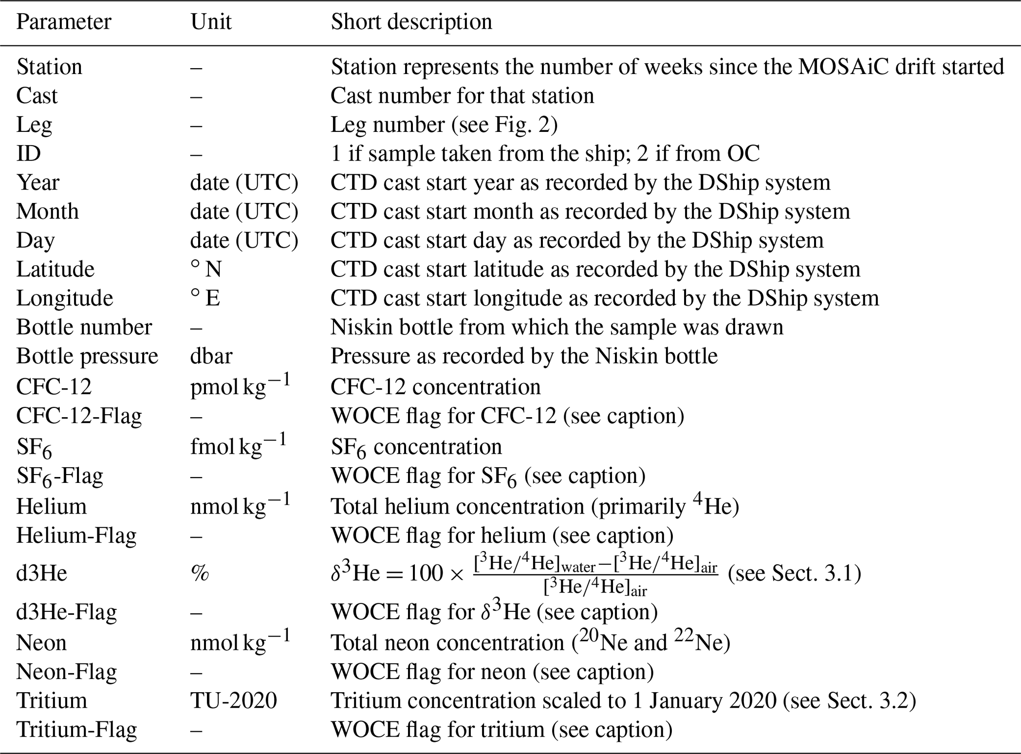
Table 2Summary of the data included in the snow data set (Huhn et al., 2023b). The World Ocean Circulation Experiment (WOCE) flags are the following: 2 = good; 3 = doubtful; 4 = bad; 6 = mean of replicates; 9 = no measurement.
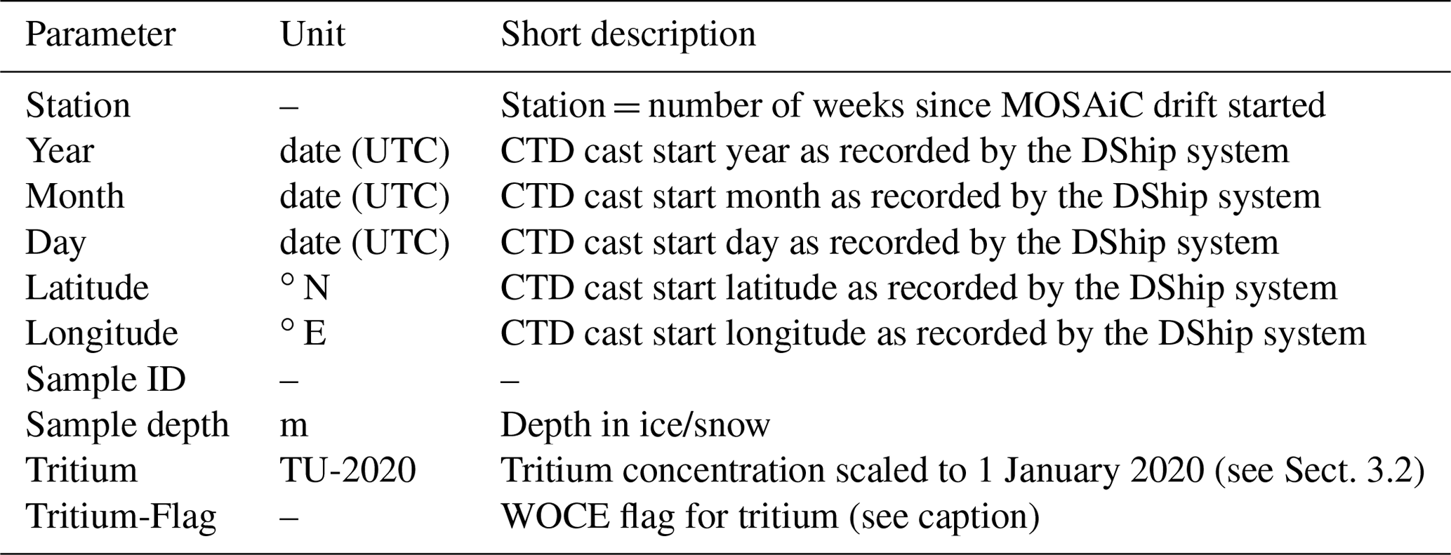
The data set metadata are identical to those of the MOSAiC CTD data sets, also on PANGAEA as Tippenhauer et al. (2023b) and Tippenhauer et al. (2023a), to facilitate cross-analysis. The link to the CTD data sets is also provided on the pages of our data sets and in the “Data availability” section of this paper. Our metadata are (see Tables 1 and 2):
-
the station (or MOSAiC week) and cast numbers,
-
the MOSAiC leg number,
-
the start date of the CTD cast,
-
the start latitude and longitude of the CTD cast, and
-
the Niskin bottle number and its recorded pressure for the ocean samples and a sample number and its depth in snow/ice for the snow samples.
We also provide an ID variable to indicate whether the sample was collected from the ship or OC CTD (two different CTD data sets). The ocean data set contains first all ship data and then all OC data.
For all variables, we use the quality flags of the World Ocean Circulation Experiment (WOCE), where 2 indicates a good value, 3 indicates doubtful, 4 indicates bad, 6 indicates that the value is the mean of several replicates, and 9 indicates that there is no measurement.
In this section, we verify that our measured values are sensible and demonstrate possible applications of these tracers for scientific studies. We show four full-depth profiles: two in the central Arctic Ocean collected in late August 2020 and two in Fram Strait collected 1 month earlier. For each region, we compare the profiles to each other and to historical values, and we finally compare the two regions.
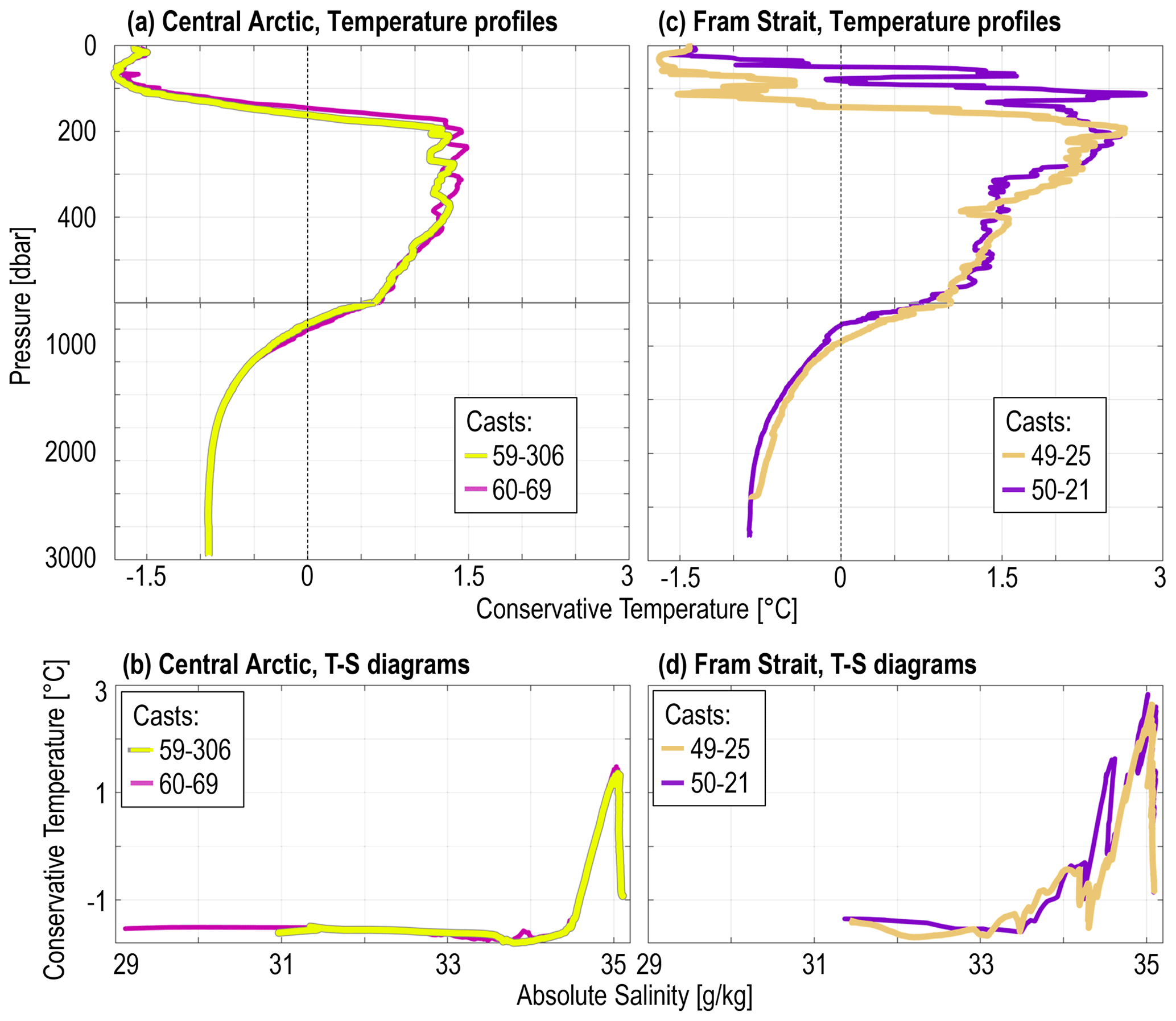
Figure 6For the two profiles of the central Arctic analysed in Sect. 5.1 (a, b) and the two Fram Strait profiles analysed in Sect. 5.2 (c, d), full-depth profiles of conservative temperature (a, c) and conservative temperature vs. absolute salinity diagram (b, d). Note the discontinued y axis on the temperature profiles. Black vertical lines in panels (a) and (c) at 0 ∘C indicates the limits of the Atlantic Water. On the T–S diagrams, the ocean surface is to the bottom left, and depth increases as the line moves towards increasing salinity.
Profiles for the historical comparison were selected from the Global Ocean Data Analysis Project (GLODAPv2; Lauvset et al., 2022, dark grey in Fig. 4). In Fram Strait, the main criterion was to remain in the deep parts of the Greenland Sea, i.e. east of the 500 m isobath and west of the prime meridian. The GLODAPv2 profiles are at most 50 km from the centre coordinate of the two studied MOSAiC profiles in Sect. 5.2. As GLODAPv2 has no noble gas data in Fram Strait, we compare our values to those collected during PS100 (also known as ARK-XXX/2; light grey in Fig. 4), published in Huhn et al. (2021b). In the central Arctic where historical values are rarer, we selected all CFC-12 and SF6 profiles in GLODAPv2 that are within 200 km of those studied in Sect. 5.1, in the deep Amundsen Basin (depth >3500 m). This yielded 12 profiles to compare to. To our knowledge, no public domain data set for noble gases contains data in the central Arctic; therefore, we limit our comparison to values from the literature. Similarly, although we acknowledge the existence of tritium data in the Arctic in the Jenkins et al. (2019) data set, we cannot use them for direct quantitative comparison as they have been decay-corrected to 1997, i.e. approximately two tritium half-lives ago.
To facilitate the discussion, we also provide the corresponding full-depth Conservative Temperature profiles as well as the Conservative Temperature vs. Absolute Salinity (T–S) diagrams (Fig. 6). More information about these variables can be found in the MOSAiC OCEAN overview (Rabe et al., 2022), which also details how to derive the mixed layer depth and Atlantic Water properties. All profiles have a shallow mixed layer not exceeding 10 m, which is to be expected for summer profiles. The Atlantic Water core (temperature maximum around 200 dbar in Fig. 6a and c or peak to the right of panels b and d) is deeper and colder for the central Arctic profiles than for the Fram Strait ones. We therefore expect tracers to show that the Atlantic Water is older in the central Arctic Ocean than in Fram Strait. The Fram Strait casts are supposedly in the Arctic outflow, i.e. should be the oldest, but instead are most likely recirculating young water. We will discuss this further in Sect. 5.3. The strong difference in surface salinity between the two casts of the central Arctic (bottom left of Fig. 6d) is discussed in Sect. 5.1. The casts of Fram Strait have many intrusions in their upper 200 m, which we discuss in Sect. 5.2. Although this does not affect our results, the reader should bear in mind that the hydrography is that of the downcast, when the water column is least perturbed, but the samples were collected during the upcast. The two do not match perfectly, especially in layers with active mixing or intrusions.
5.1 Profile agreement in the central Arctic
The two profiles in the central Arctic Ocean have the cast numbers 59-306 (bright yellow on all figures) and 60-69 (purple/magenta). They are 80 km apart. Both casts were collected while R/V Polarstern was moored to the ice, 59-306 on 27 August 2020 and 60-69 on 3 September 2020. Tritium was collected only during cast 59-306. Helium, neon, and tritium were collected in the upper 500 m only; CFC-12 and SF6 were collected down to the sea floor, approximately 4400 m deep.
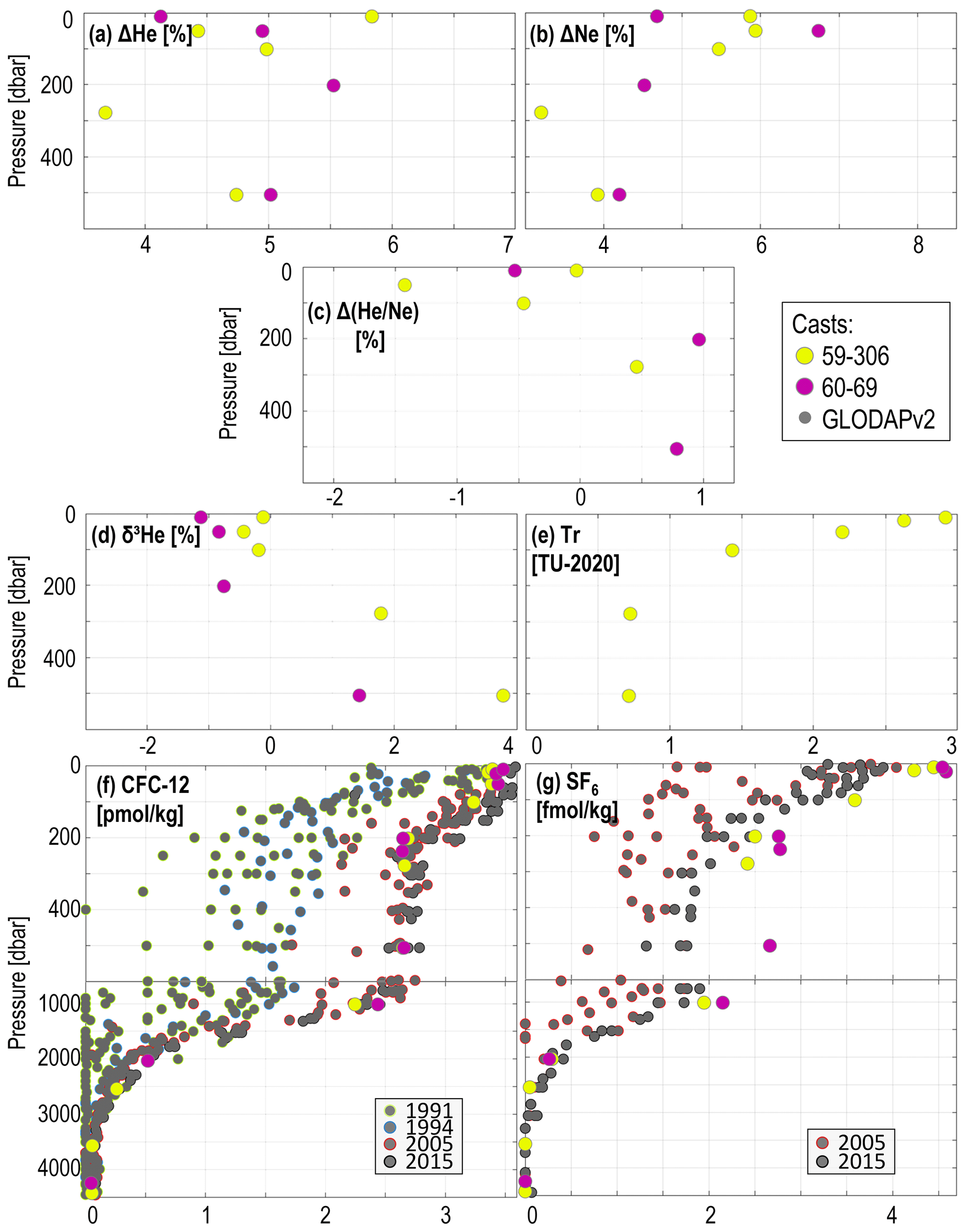
Figure 7Two exemplary profiles collected a week and 80 km apart in the central Arctic Ocean in summer 2020 during MOSAiC for (a) helium, (b) neon, (c) helium to neon ratio, (d) 3He, (e) tritium, (f) CFC-12 concentration, and (g) SF6 concentration. Grey dots are reference values from GLODAPv2 if available. See locations in Fig. 4.
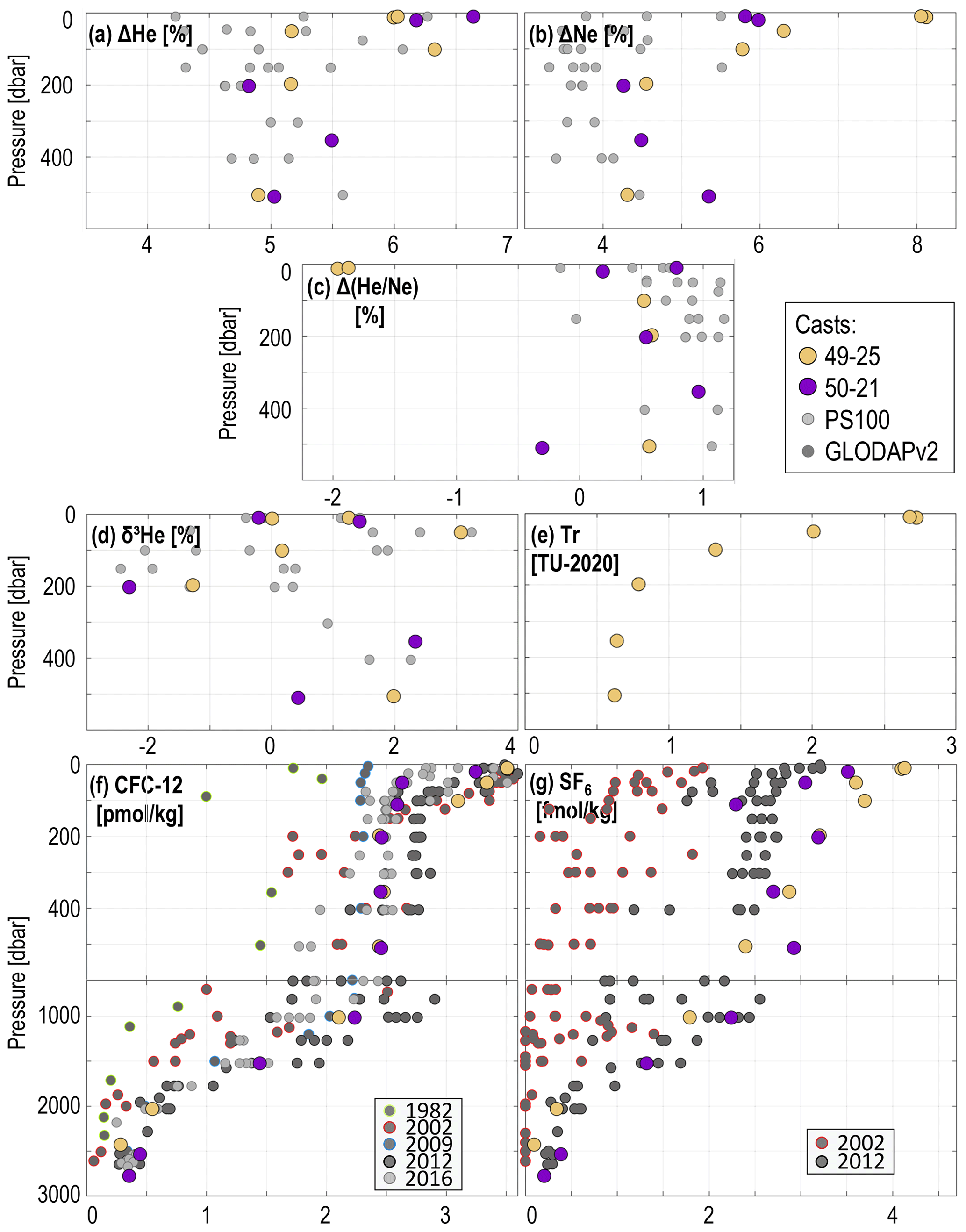
Figure 8Two exemplary profiles collected a week and 72 km apart in Fram Strait in summer 2020 during MOSAiC for (a) helium, (b) neon, (c) helium to neon ratio, (d) 3He, (e) tritium, (f) CFC-12 concentration, and (g) SF6 concentration. Grey dots are reference values from PS100 (pale grey, all variables except SF6) and GLODAPv2 (dark grey, CFC-12 and SF6; coloured contours indicate the year) if available. See locations in Fig. 4.
The upper 100 m is very different for both profiles for helium, neon, and their ratio (Fig. 7a–c). Starting with cast 59-306 (yellow), we observe a zigzag pattern in helium, decreasing significantly from 5.8 % at 10 m depth to 4.4 % at 50 m only to increase again to 5 % at 100 m. Changes in neon are less strong but follow the opposite pattern: increase then decrease. Consequently, the ratio goes from nearly 0 % at the surface to −1.4 % at 50 m and increases afterwards. The signal around 50 m could indicate a by-product of the previous autumn's sea ice formation, which was carried with the mixed layer in the previous winter when it was deeper and was trapped below the shallow summer mixed layer (approx 10 m deep). A week later in contrast, cast 60-69 (purple) has low He and Ne at the surface, which both increase below. The surface salinity is approx. 2 g kg−1 fresher for cast 60-69 than for cast 59-306 taken a week prior (Fig. 6d), which suggests that the ice has melted between the two casts and/or that the ship has drifted into different surface waters. Finally, the very different values between the two casts at 300 m (59-306) and 200 m (60-69) indicate that the samples happen to be taken in different waters, which is consistent with the large intrusions in that depth range (Fig. 6c).
The two casts do not show significant differences in the upper 50 m in the 3He signals (Fig. 7d), with differences within the measurement error range. For both casts, 3He then increases with depth, most likely as a result of tritium decay, as expected for that depth range in the central Arctic Ocean.
At the surface, the water is at the same temperature (−1.5∘C) in both casts, but the salinity differed by 2 g kg−1 (Fig. 6d). Hence, we expect a solubility difference on the order of 0.1 pmol kg−1 for CFC-12 and 0.1 fmol kg−1 for SF6, which is consistent with the observed differences in concentration between the two casts at 10 and 20 m depth for CFC-12 (Fig. 7f) and at 10 m depth for SF6 (Fig. 7g). The difference at 20 m in SF6 is 0.35 or 3 times as high as expected from the solubility difference only; the corresponding density (not shown) indicates a small instability at that depth, so the gas deficit could be caused by mild overturning. At 50 m, the salinity difference between the two profiles taken a week apart decreases by a factor of 10 while the temperature remains similar; from solubility alone, the difference in CFC-12 between the two profiles should be 0.01 pmol kg−1, but it remains at 0.1. There is no SF6 value at that depth, but in agreement with the strong stratification evidenced by, for example, the signal, this difference might still reflect the solubility difference when the waters of these two profiles were at the surface. Below, in the Atlantic Water layer, the two profiles have somewhat constant and similar values in both CFC-12 and SF6. Differences could come, as explained above, from sampling of different waters in the intrusions, which is not surprising for profiles collected 1 week and 80 km apart. Interestingly, in the bottom 1000 m, both profiles have values above the detection threshold for CFC-12 (Fig. 7f) but below the detection threshold for SF6 (Fig. 7g). This suggests that these waters were last at the surface in the 1930s, when CFC-12 was already used but industrial usage of SF6 was still in its infancy. The historical CFC-12 data clearly show two different regimes, especially so in the upper 1000 m, with our profiles fitting nicely in between (Fig. 7f). The historical SF6 values are consistently lower than ours (Fig. 7g). Although not specified in Fig. 4 for readability, not all GLODAPv2 profiles had both CFC-12 and SF6, so the reference SF6 profiles are systematically further towards the central Amundsen Basin than ours. They also were collected 15 to 30 years before ours, and the reader should bear in mind that SF6 is still increasing in the atmosphere. It is therefore no surprise that these reference profiles have lower SF6 values than ours.
Huhn et al. (2023a)Huhn et al. (2023b)Tippenhauer et al. (2023b)Tippenhauer et al. (2023a)Jakobsson et al. (2020)Huhn et al. (2021b)Lauvset et al. (2022)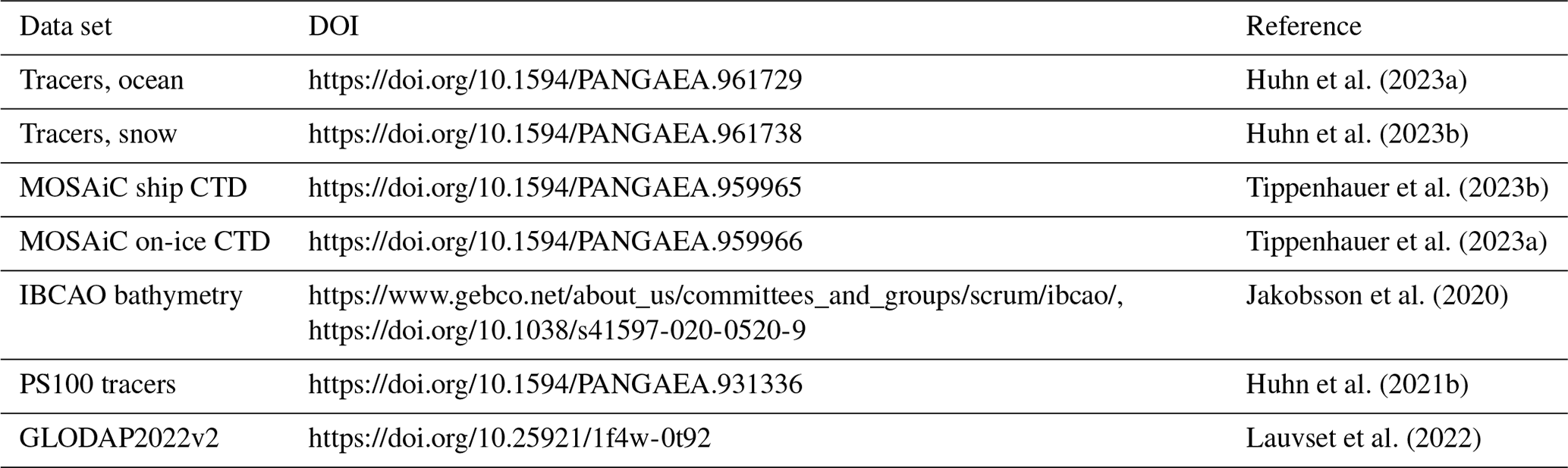
5.2 Profile agreement in Fram Strait
The two profiles in Fram Strait have the cast numbers 49-25 (orange/yellow in all figures) and 50-21 (purple). They are 72 km away from each other. Cast 49-25 was collected on 29 July 2020 while R/V Polarstern was still moored at the ice floe; cast 50-21 was collected on 5 August 2020 during transit. Tritium was collected only during cast 49-25. Helium, neon, and tritium were collected in the upper 500 m only; CFC-12 and SF6 were collected down to the sea floor, approximately 3000 m deep. Note that Fram Strait is well-known for its variability in both space and time. To better understand the dynamics and processes in Fram Strait, a data set with better spatio-temporal resolution would be required, such as the one described in Stöven et al. (2016). Here we only describe, briefly, some noteworthy features of the profiles.
The first cast, 49-25, has a low value of around −2 % at the surface (Fig. 8c), steadily increasing for the rest of the profile, whereas the second cast, 50-21, is positive at the surface and more inconsistent throughout the profile. The negative values at the surface for cast 49-25 could be the result of sea ice formation, although the air temperatures reported in Shupe et al. (2022) were hovering around 0 ∘C in the week leading to cast 49-25, which rather suggests sea ice melt. Verifying whether sea ice formation actually took place is beyond the scope of this data paper. The increased helium value around 350 m in cast 50-21 (Fig. 8a, purple) could indicate the presence of Greenland meltwater (Huhn et al., 2021a), but is more likely not significant. Note that all values are within the range observed during PS100 (grey dots; also see Table 3), with somewhat higher values for neon during MOSAiC (Fig. 8b), further suggesting sea ice formation. Neon, 3He, and tritium all have a sharp decline in the upper 200 m, highlighting the transition into Atlantic Water (Fig. 6 compared to Fig 8).
Finally, below the Atlantic Water and down to the sea floor, the CFC-12 and SF6 concentrations (Fig. 8f and g) are lower for cast 49-25 (yellow) than for cast 50-21 (purple), and cast 49-25 is also warmer. However, the difference persists when comparing the partial pressure (not shown). The differences are more likely caused by different water masses and/or different (re)circulation, but more data would be required to establish this. Although both variables, for both casts, are within the range of PS100 and GLODAPv2 data, it is worth noting that SF6 in GLODAPv2 is very noisy and that the data quality seems variable.
5.3 Brief comparison of the two regions
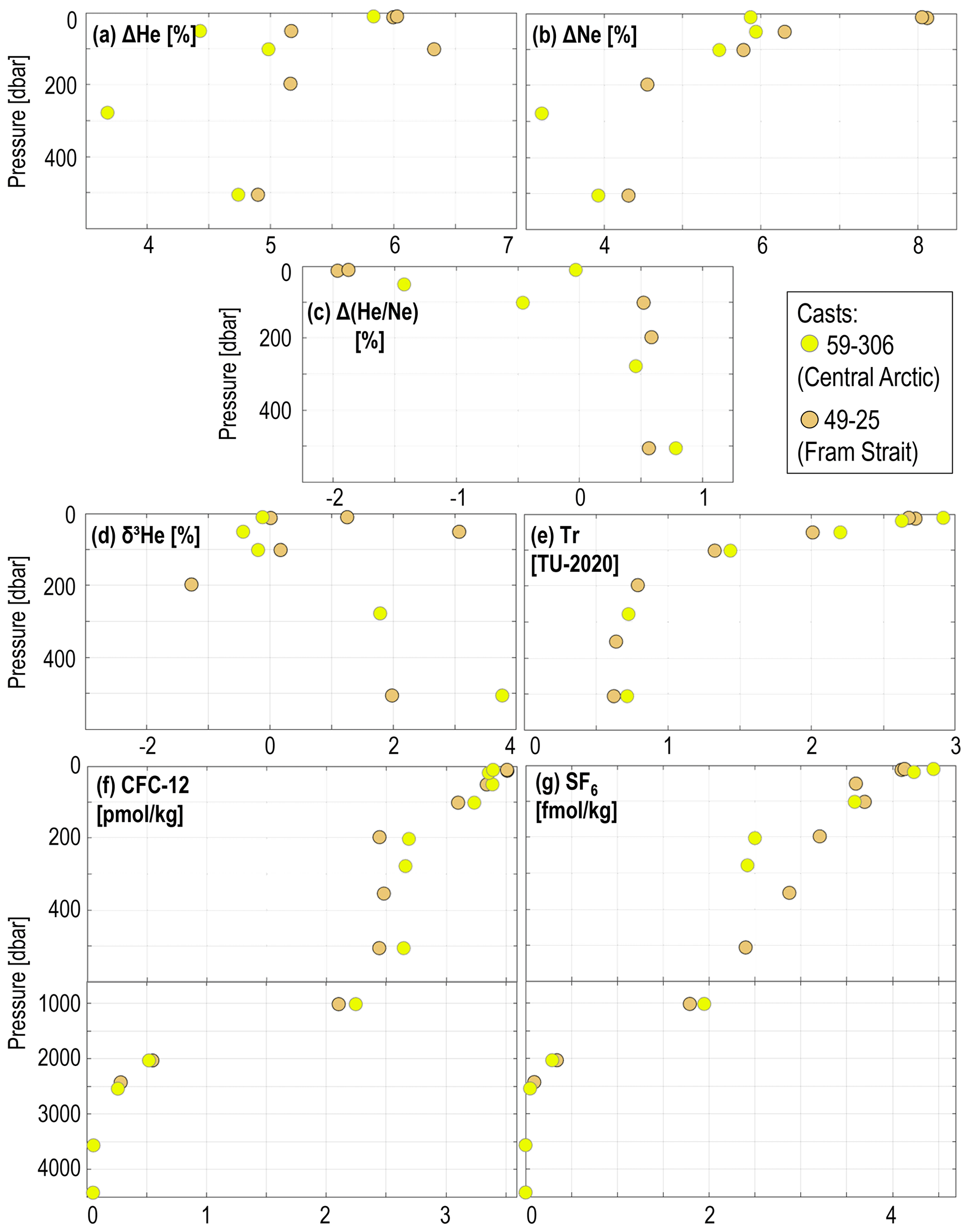
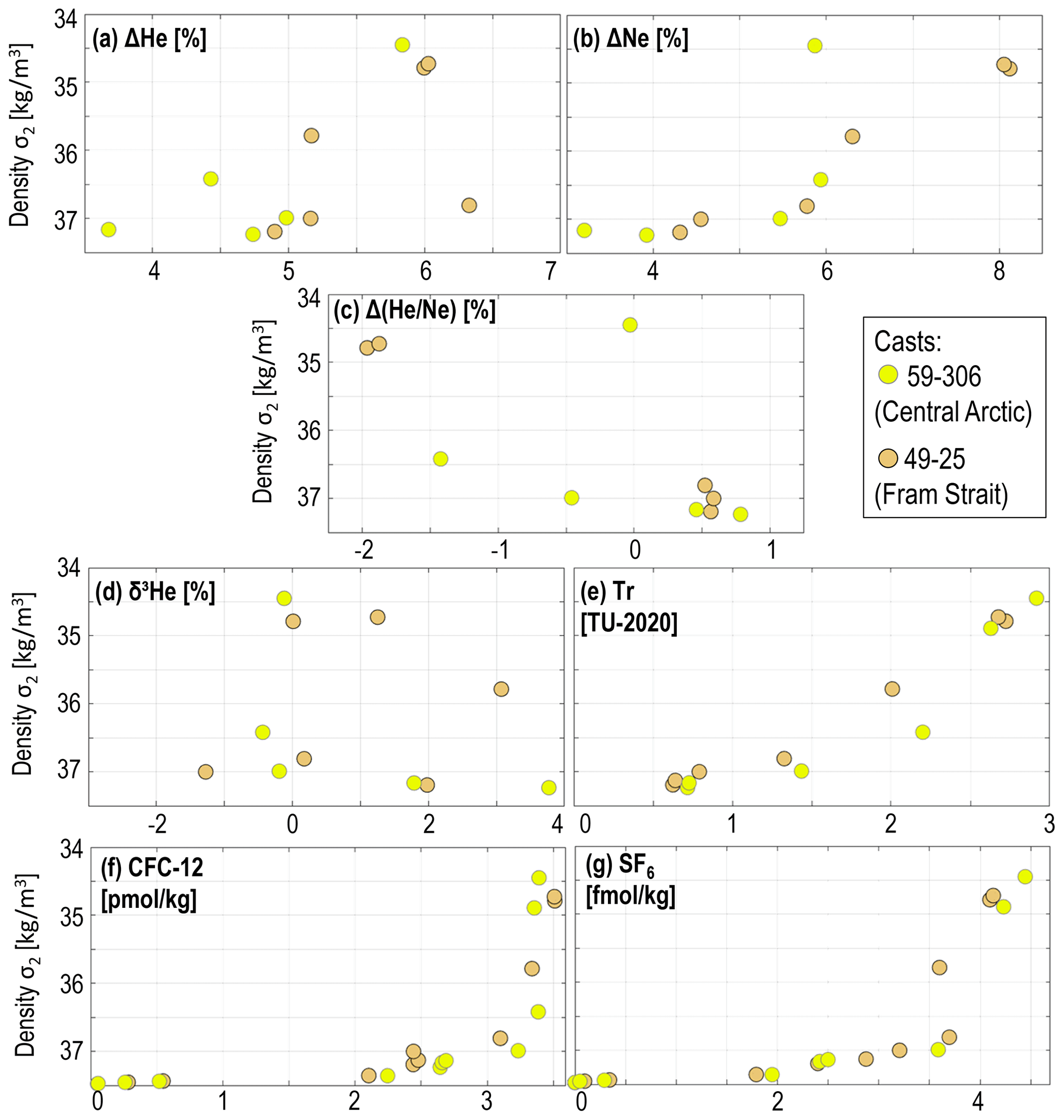
We now briefly compare profile 59-306 of the central Arctic with profile 49-25 of Fram Strait, as they both have measurements for all tracers, including tritium. We chose summer profiles for both regions to try and minimise the effect of seasonality, but we acknowledge that disentangling the temporal and spatial variability may not be straightforward for some applications. In particular, we do not comment further on helium and neon (Fig. 9a–c), as the differences between the two locations is most likely caused by seasonal sea ice processes, as we discussed previously. The profiles are also provided as a function of density in Fig. A1.
The central Arctic Ocean cast 59-306 has systematically larger values of tritium than the Fram Strait cast 49-25 (Fig. 9e), which is to be expected as the central Arctic is closer to the sources of tritium: rivers flowing onto the Arctic shelf (e.g. Schlosser et al., 1994). Nothing happens aside from the expected decrease in value with depth, as expected from profiles that are not directly influenced by a river outflow.
From approx. 300 m depth, i.e. in the Atlantic Water, the larger 3He values (Fig. 9d) for the central Arctic Ocean than for Fram Strait are consistent with the larger tritium we just described. Besides, as the seafloor lies 4000 m away from our measurements, 3He is unlikely to come from the mantle. Along with the lower SF6 for the central Arctic (Fig. 9g) over approx. 200 to 500 m depth, these larger 3He values rather suggest that the waters in the Atlantic Water are older in the central Arctic than they are in Fram Strait. That is, the water now at approx 200–500 m depth in the central Arctic Ocean were last at the surface in the North Atlantic a longer time ago than those now in Fram Strait. This is consistent with the difference in hydrography (Fig. 6), as described at the beginning of this section: although on the western side of Fram Strait, our Fram Strait profile contains young water. The tracers and hydrography therefore indicate a recirculation in Fram Strait (e.g. Hofmann et al., 2021), extending to the sampling location.
All data used in this paper are listed in Table 3.
In this manuscript, we describe the CFC-12, SF6, tritium, helium, and neon data set produced from the samples collected between October 2019 and September 2020 during the MOSAiC expedition to the Eurasian Arctic Ocean. Noble gases and tritium were limited to the upper 500 m, whereas CFC-12 and SF6 were collected for the full depth. All tracers are available at weekly or higher temporal resolution, although CFC-12 and SF6 are limited to the upper 1000 m during the 2-month period (March–May 2020) where the ship CTD could not be operated. We showed that individual tracers can be used or combined with each other to investigate rapid sea ice processes, the (suspected) ocean mixing, and even the presence of oceanic recirculation branches. By studying them in relation to sparse, previously collected data (or other tracers), they can be used to study the large-scale oceanic circulation or even elucidate the impact of climate change on ventilation.
Unsurprisingly, the main conclusion for us is that we regret not collecting more samples. Having a larger team and/or more experienced samplers would have allowed us to collect tracers at a higher vertical resolution. The ice dynamics made the ship CTD inoperable during 2 months, which coincided with the transition from the Amundsen Basin to the Nansen Basin via Gakkel Ridge. This possibility had been foreseen during the MOSAiC planning phase, so an alternative water collection system via the moon pool had been devised but ultimately not implemented as it was too expensive. Besides, due to the objectives of the contributing projects, the funding for noble gases and tritium, which can be used to track hydrothermal plumes and ventilation, respectively, was limited to the upper 500 m.
As the Arctic, a hotspot of climate change, becomes the focal point of many teams and funding agencies, we strongly recommend that future endeavours collect samples of these tracers all the way to the sea floor, especially so in the vicinity of Gakkel Ridge and close to suspected overflow locations (listed in, for example, Luneva et al., 2020).
The different gases require a different solubility function to determine the response of their solubility to changes in temperature and salinity. For He and Ne, it is that of Weiss (1971); for CFC-12 it is that of Warner and Weiss (1985); and for SF6 it is that of Bullister et al. (2002). These yield the following:
-
At a fixed salinity of 34 psu, for a change in temperature from 1 to 0 ∘C, He increases by 0.5 %, Ne increases by 0.9 %, CFC-12 increases by 6 %, and SF6 increases by 5 %;
-
At a fixed temperature of 1 ∘C, for a change in salinity from 33 to 34 psu, He increases by 0.6 %, Ne increases by 0.7 %, CFC-12 increases by 1 %, and SF6 increases by 1 %.
That is, CFC-12 and SF6 are up to 10 times more affected by a change in temperature than He and Ne, but they all have a similar response to a change in salinity.
The gas exchange between ocean and atmosphere depends on the gradient between the two, the wind velocity, the solubility, etc. The velocity of the exchange, Vg, depends primarily on the Schmidt number Sc, as described in, for example, Wanninkhof (1992):
Using an average wind speed uav of 3 m s−1, we obtain
-
For He, Sc = 372, so Vg = 13 cm h−1.
-
For Ne, Sc = 767, so Vg = 9 cm h−1.
-
For CFC-12, Sc = 3256, so Vg = 4.4 cm h−1.
-
For SF6, Sc = 3000, so Vg = 4.6 cm h−1.
That is, He and Ne are 2 to 3 times faster equilibrated than CFC-12 and SF6.
Initial conception of the study: CH, OH and MW. Fieldwork logistics and/or collection of samples: JA, YCF, HH, CH, SK, DK, IK, MM, CM, BR, NS, ST. Lab analysis of the samples: KB, OH, JS. Preparation of the original draft, including visualisations: KB, CH, OH, SK, WK, JS, MV, MW. Initial submission: all.
The contact author has declared that none of the authors has any competing interests.
Publisher’s note: Copernicus Publications remains neutral with regard to jurisdictional claims made in the text, published maps, institutional affiliations, or any other geographical representation in this paper. While Copernicus Publications makes every effort to include appropriate place names, the final responsibility lies with the authors.
Data used in this paper were produced as part of the international Multidisciplinary drifting Observatory for the Study of the Arctic Climate (MOSAiC) expedition with the tag MOSAiC20192020 (AWI_PS122_00). We thank all those who contributed to MOSAiC and made this endeavour possible (Nixdorf et al., 2021). Céline Heuzé and Salar Karam were supported by Vetenskapsrådet (grant no. 2018-03859), awarded to Céline Heuzé, for project “Why is the deep Arctic Ocean Warming? (WAOW)”, and we acknowledge support from the Swedish Polar Research Secretariat for berth fees for MOSAiC. Wiebke Körtke, Natalia Sukhikh, and Maren Walter gratefully acknowledge the funding by the Deutsche Forschungsgemeinschaft (DFG, German Research Foundation) (project no. 268020496–TRR 172), within the Transregional Collaborative Research Center “ArctiC Amplification: Climate Relevant Atmospheric and SurfaCe Processes, and Feedback Mechanisms (AC)3”. This work contributes to the Changing Arctic Ocean (CAO) programme, jointly funded by the UKRI Natural Environment Research Council (NERC) and the BMBF, project Advective Pathways of nutrients and key Ecological substances in the ARctic (APEAR) (grants NE/R012865/1, NE/R012865/2 and #03V01461); and the BMBF project Eddy Properties and Impacts in the Changing Arctic (EPICA) (grant no. 03F0889A). Hailun He is funded by the Chinese Polar Environmental Comprehensive Investigation and Assessment Programs. We thank the two anonymous reviewers whose comments greatly improved the quality of the paper.
This research has been supported by the Vetenskapsrådet (grant no. 2018-03859) and the Deutsche Forschungsgemeinschaft (grant no. 268020496–TRR 172).
The article processing charges for this open-access publication were covered by the Gothenburg University Library.
This paper was edited by Dagmar Hainbucher and reviewed by Núria Casacuberta and one anonymous referee.
Beaird, N., Straneo, F., and Jenkins, W.: Spreading of Greenland meltwaters in the ocean revealed by noble gases, Geophys. Res. Lett., 42, 7705–7713, https://doi.org/10.1002/2015GL065003, 2015. a, b
Bullister, J., Wisegarver, D., and Menzia, F.: The solubility of sulfur hexafluoride in water and seawater, Deep-Sea Res. Pt. I, 49, 175–187, https://doi.org/10.1016/S0967-0637(01)00051-6, 2002. a
Bullister, J. L.: Atmospheric Histories (1765–2015) for CFC-11, CFC-12, CFC-113, CCl4, SF6 andN2O, https://doi.org/10.3334/CDIAC/otg.CFC_ATM_Hist_2015, 2015. a
Bulsiewicz, K., Rose, H., Klatt, O., Putzka, A., and Roether, W.: A capillary‐column chromatographic system for efficient chlorofluorocarbon measurement in ocean waters, J. Geophys. Res.-Oceans, 103, 15959–15970, https://doi.org/10.1029/98JC00140, 1998. a, b
Curren, T.: Nuclear-powered Submarines: Potential Environmental Effects, https://inis.iaea.org/collection/NCLCollectionStore/_Public/24/010/24010563.pdf (last access: 21 September 2023), 1988. a
Dutton, G. S., Hall, B., Dlugokencky, E., Lan, X., Nance, J., Gentry, M., and Madronich, M.: Combined Atmospheric Sulfur hexaflouride Dry Air Mole Fractions from the NOAA GML Halocarbons Sampling Network, 1995–2022, version: 2022-08-12, NOAA [data set], https://doi.org/10.15138/TQ02-ZX42, 2022a. a
Dutton, G. S., Hall, B., Montzka, S., Nance, J., and Gentry, M.: Combined Atmospheric Chloroflurocarbon-12 Dry Air Mole Fractions from the NOAA GML Halocarbons Sampling Network, 1977–2022, version: 2022-08-12, NOAA [data set], https://doi.org/10.15138/PJ63-H440, 2022b. a
Ebser, S., Kersting, A., Stöven, T., Feng, Z., Ringena, L., Schmidt, M., Tanhua, T., Aeschbach, W., and Oberthaler, M.: 39Ar dating with small samples provides new key constraints on ocean ventilation, Nat. Commun., 9, 5046, https://doi.org/10.1038/s41467-018-07465-7, 2018. a
Fine, R.: Observations of CFCs and SF6 as Ocean Tracers, Annu. Rev. Mar. Sci., 3, 173–195, https://doi.org/10.1146/annurev.marine.010908.163933, 2011. a
German, C., Reeves, E., Türke, A., Diehl, A., Albers, E., Bach, W., Purser, A., Ramalho, S., Suman, S., Mertens, C., Walter, M., Ramirez-Llodra, E., Schlindwein, V., Bünz, S., and Boetius, A.: Volcanically hosted venting with indications of ultramafic influence at Aurora hydrothermal field on Gakkel Ridge, Nat. Commun., 13, 6517, https://doi.org/10.1038/s41467-022-34014-0, 2022. a
Hahm, D., Postlethwaite, C. F., Tamaki, K., and Kim, K. R.: Mechanisms controlling the distribution of helium and neon in the Arctic seas: The case of the Knipovich Ridge, Earth Planet. Sc. Lett., 229, 125–139, https://doi.org/10.1016/j.epsl.2004.10.028, 2004. a, b
Heuzé, C., Purkey, S. G., and Johnson, G. C.: It is high time we monitor the deep ocean, Environ. Res. Lett., 17, 121002, https://doi.org/10.1088/1748-9326/aca622, 2022. a
Hofmann, Z., von Appen, W.-J., and Wekerle, C.: Seasonal and Mesoscale Variability of the Two Atlantic Water Recirculation Pathways in Fram Strait, J. Geophys. Res.-Oceans, 126, e2020JC017057, https://doi.org/10.1029/2020JC017057, 2021. a
Huhn, O., Rhein, M., Kanzow, T., Schaffer, J., and Sültenfuß, J.: Submarine meltwater from Nioghalvfjerdsbrae (79 north Glacier), northeast Greenland, J. Geophys. Res.-Oceans, 126, e2021JC017224, https://doi.org/10.1029/2021JC017224, 2021a. a, b, c
Huhn, O., Rhein, M., Bulsiewicz, K., and Sültenfuß, J.: Noble gas (He, Ne isotopes) and transient tracer (CFC-11 and CFC-12) measurements from POLARSTERN cruise PS100 (northeast Greenland, 2016), PANGAEA [data set], https://doi.org/10.1594/PANGAEA.931336, 2021b. a, b
Huhn, O., Heuzé, C., Walter, M., Mertens, C., Bulsiewicz, K., and Sültenfuß, J.: Transient tracers (CFC-12 and SF6), noble gases (He and Ne isotopes), and Tritium measurements from POLARSTERN cruise PS122 (MOSAiC, 2019–2020), PANGAEA [data set], https://doi.org/10.1594/PANGAEA.961729, 2023a. a, b, c
Huhn, O., Heuzé, C., Walter, M., Mertens, C., Bulsiewicz, K., and Sültenfuß, J.: Tritium in snow measurements from POLARSTERN cruise PS122 (MOSAiC, 2019–2020), PANGAEA [data set], https://doi.org/10.1594/PANGAEA.961738, 2023b. a, b, c
Jakobsson, M., Mayer, L. A., Bringensparr, C., Castro, C. F., Mohammad, R., Johnson, P., Ketter, T., Accettella, D., Amblas, D., An, L., Arndt, J. E., Canals, M., Casamor, J. L., Chauché, N., Coakley, B., Danielson, S., Demarte, M., Dickson, M. L., Dorschel, B., Dowdeswell, J. A., Dreutter, S., Fremand, A. C., Gallant, D., Hall, J. K., Hehemann, L., Hodnesdal, H., Hong, J., Ivaldi, R., Kane, E., Klaucke, I., Krawczyk, D. W., Kristoffersen, Y., Kuipers, B. R., Millan, R., Masetti, G., Morlighem, M., Noormets, R., Prescott, M. M., Rebesco, M., Rignot, E., Semiletov, I., Tate, A. J., Travaglini, P., Velicogna, I., Weatherall, P., Weinrebe, W., Willis, J. K., Wood, M., Zarayskaya, Y., Zhang, T., Zimmermann, M., and Zinglersen, K. B.: The International Bathymetric Chart of the Arctic Ocean Version 4.0, Scientific Data, 7, 176, https://doi.org/10.1038/s41597-020-0520-9, 2020 (data available at: https://www.gebco.net/about_us/committees_and_groups/scrum/ibcao/, last access: 30 November 2023). a, b, c
Jenkins, W., Lott III, D., Longworth, B., Curtice, J., and Cahill, K.: The distributions of helium isotopes and tritium along the US GEOTRACES North Atlantic sections (GEOTRACES GAO3), Deep-Sea Res. Pt. II, 116, 21–28, https://doi.org/10.1016/j.dsr2.2014.11.017, 2015. a
Jenkins, W. J., Doney, S. C., Fendrock, M., Fine, R., Gamo, T., Jean-Baptiste, P., Key, R., Klein, B., Lupton, J. E., Newton, R., Rhein, M., Roether, W., Sano, Y., Schlitzer, R., Schlosser, P., and Swift, J.: A comprehensive global oceanic dataset of helium isotope and tritium measurements, Earth Syst. Sci. Data, 11, 441–454, https://doi.org/10.5194/essd-11-441-2019, 2019. a
Johnson, G. C., Hosoda, S., Jayne, S. R., Oke, P. R., Riser, S. C., Roemmich, D., Suga, T., Thierry, V., Wijffels, S. E., and Xu, J.: Argo–Two decades: Global oceanography, revolutionized, Annu. Rev. Mar. Sci., 14, 379–403, https://doi.org/10.1146/annurev-marine-022521-102008, 2022. a
Knust, R.: Polar Research and Supply Vessel POLARSTERN Operated by the Alfred-Wegener-Institute, Journal of Large-Scale Research Facilities, 3, A119, https://doi.org/10.17815/jlsrf-3-163, 2017. a
Koeve, W., Wagner, H., Kähler, P., and Oschlies, A.: 14C-age tracers in global ocean circulation models, Geosci. Model Dev., 8, 2079–2094, https://doi.org/10.5194/gmd-8-2079-2015, 2015. a
Kwok, R.: Arctic sea ice thickness, volume, and multiyear ice coverage: losses and coupled variability (1958–2018), Environ. Res. Lett., 13, 105005, https://doi.org/10.1088/1748-9326/aae3ec, 2018. a
Lauvset, S. K., Lange, N., Tanhua, T., Bittig, H. C., Olsen, A., Kozyr, A., Alin, S. R., Álvarez, M., Azetsu-Scott, K., Barbero, L., Becker, S., Brown, P. J., Carter, B. R., Cotrim da Cunha, L., Feely, R. A., Hoppema, M., Humphreys, M. P., Ishii, M., Jeansson, E., Jiang, L.-Q., Jones, S. D., Lo Monaco, C., Murata, A., Müller, J. D., Pérez, F. F., Pfeil, B., Schirnick, C., Steinfeldt, R., Suzuki, T., Tilbrook, B., Ulfsbo, A., Velo, A., Woosley, R. J., and Key, R. M.: Global Ocean Data Analysis Project version 2.2022 (GLODAPv2.2022) (NCEI Accession 0257247), NOAA [data set], https://doi.org/10.25921/1f4w-0t92, 2022. a, b
Loose, B. and Jenkins, W.: The five stable noble gases are sensitive unambiguous tracers of glacial meltwater, Geophys. Res. Lett., 41, 2835–2841, https://doi.org/10.1002/2013GL058804, 2014. a
Luneva, M., Ivanov, V., Tuzov, F., Aksenov, Y., Harle, J., Kelly, S., and Holt, J.: Hotspots of dense water cascading in the Arctic Ocean: Implications for the Pacific water pathways, J. Geophys. Res.-Oceans, 125, e2020JC016044, https://doi.org/10.1029/2020JC016044, 2020. a
Mauldin, A., Schlosser, P., Newton, R., Smethie Jr, W., Bayer, R., Rhein, M., and Jones, E.: The velocity and mixing time scale of the Arctic Ocean Boundary Current estimated with transient tracers, J. Geophys. Res.-Oceans, 115, C08002, https://doi.org/10.1029/2009JC005965, 2010. a
Meredith, M., Sommerkorn, M., Cassotta, S., Derksen, C., Ekaykin, A., Hollowed, A., and et al., K. G.: IPCC Special Report on the Ocean and Cryosphere in a Changing Climate, Chapter 3, Polar Regions, UN, https://www.ipcc.ch/srocc/ (last access: 30 November 2023), 2019. a
Muilwijk, M., Nummelin, A., Heuzé, C., Polyakov, I. V., Zanowski, H., and Smedsrud, L. H.: Divergence in climate model projections of future Arctic Atlantification, J. Climate, 36, 1727–1748, https://doi.org/10.1175/JCLI-D-22-0349.1, 2023. a
Nixdorf, U., Dethloff, K., Rex, M., Shupe, M., Sommerfeld, A., Perovich, D. K., Nicolaus, M., Heuzé, C., Rabe, B., Loose, B., Damm, E., Gradinger, R., Fong, A., Maslowski, W., Rinke, A., Kwok, R., Spreen, G., Wendisch, M., Herber, A., Hirsekorn, M., Mohaupt, V., Frickenhaus, S., Immerz, A., Weiss-Tuider, K., König, B., Mengedoht, D., Regnery, J., Gerchow, P., Ransby, D., Krumpen, T., Morgenstern, A., Haas, C., Kanzow, T., Rack, F. R., Saitzev, V., Sokolov, V., Makarov, A., Schwarze, S., Wunderlich, T., Wurr, K., and Boetius, A.: MOSAiC Extended Acknowledgement, Zenodo [data set], https://doi.org/10.5281/zenodo.5541624, 2021. a
Oms, P., Du Bois, P., Dumas, F., Lazure, P., Morillon, M., Voiseux, C., Le Corre, C., Cossonnet, C., Solier, L., and Morin, P.: Inventory and distribution of tritium in the oceans in 2016, Sci. Total Environ., 656, 1289–1303, https://doi.org/10.1016/j.scitotenv.2018.11.448, 2019. a
Polyakov, I. V., Pnyushkov, A. V., and Carmack, E. C.: Stability of the Arctic halocline: a new indicator of Arctic climate change, Environ. Res. Lett., 13, 125008, https://doi.org/10.1088/1748-9326/aaec1e, 2018. a
Polyakov, I. V., Alkire, M. B., Bluhm, B. A., Brown, K. A., Carmack, E. C., Chierici, M., and Danielson, M. C. E.: Borealization of the Arctic Ocean in response to anomalous advection from sub-Arctic seas, Frontiers in Marine Science, 7, 491, https://doi.org/10.3389/fmars.2020.00491, 2020. a
Prinn, R., R.F., W., Fraser, P., Simmonds, P., Cunnold, D., Alyea, F., O'Doherty, S., Salameh, P., Miller, B., Huang, J., Wang, R., Hartley, D., Harth, C., Steele, L., Sturrock, G., Midgley, P., and McCulloch, A.: A history of chemically and radiatively important gases in air deduced from ALE/GAGE/AGAGE, J. Geophys. Res.-Atmos., 105, 17751–17792, https://doi.org/10.1029/2000JD900141, 2000. a
Rabe, B., Heuzé, C., Regnery, J., Aksenov, Y., Allerholt, J., Athanase, M., Bai, Y., Basque, C., Bauch, D., Baumann, T., and Chen, D. E.: Overview of the MOSAiC expedition: Physical oceanography, Elem. Sci. Anth., 10, 00062, https://doi.org/10.1525/elementa.2021.00062, 2022. a, b, c, d
Rajasakaren, B., Jeansson, E., Olsen, A., Tanhua, T., Johannessen, T., and Smethie Jr., W.: Trends in anthropogenic carbon in the Arctic Ocean, Prog. Oceanogr., 178, 102177, https://doi.org/10.1016/j.pocean.2019.102177, 2019. a
Rhein, M., Dengler, M., Sültenfuß, J., Hummels, R., Hüttl-Kabus, S., and Bourles, B.: Upwelling and Associated Heat Flux in the Equatorial Atlantic Inferred from Helium Isotope Disequilibrium, J. Geophys. Res., 115, C08021, https://doi.org/10.1029/2009JC005772, 2010. a
Roether, W., Well, R., Putzka, A., and Rueth, C.: Component Separation of Oceanic Helium, J. Geophys. Res., 103, 27931–27946, https://doi.org/10.1029/98JC02234, 1998. a
Schlosser, P.: Helium: a new tracer in Antarctic oceanography, Nature, 321, 233–235, https://doi.org/10.1038/321233a0, 1986. a
Schlosser, P., Bönisch, G., Kromer, B., Münnich, K., and Koltermann, K.: Ventilation rates of the waters in the Nansen Basin of the Arctic Ocean derived from a multitracer approach, J. Geophys. Res.-Oceans, 95, 3265–3272, https://doi.org/10.1029/JC095iC03p03265, 1990. a
Schlosser, P., Bauch, D., Fairbanks, R., and Bönisch, G.: Arctic river-runoff: mean residence time on the shelves and in the halocline, Deep-Sea Res. Pt. I, 41, 1053–1068, https://doi.org/10.1016/0967-0637(94)90018-3, 1994. a
Shupe, M., Rex, M., Blomquist, B., Persson, P., Schmale, J., Uttal, T., Althausen, D., Angot, H., Archer, S., Bariteau, L., and Beck, I. E.: Overview of the MOSAiC expedition: Atmosphere, Elem. Sci. Anth., 10, 00060, https://doi.org/10.1525/elementa.2021.00060, 2022. a
Smith, J. N., Smethie Jr., W. M., and Casacuberta, N.: Synoptic 129I and CFC–SF6 Transit Time Distribution (TTD) Sections Across the Central Arctic Ocean From the 2015 GEOTRACES Cruises, J. Geophys. Res.-Oceans, 127, e2021JC018120, https://doi.org/10.1029/2021JC018120, 2022. a
Solomon, A., Heuzé, C., Rabe, B., Bacon, S., Bertino, L., Heimbach, P., Inoue, J., Iovino, D., Mottram, R., Zhang, X., Aksenov, Y., McAdam, R., Nguyen, A., Raj, R. P., and Tang, H.: Freshwater in the Arctic Ocean 2010–2019, Ocean Sci., 17, 1081–1102, https://doi.org/10.5194/os-17-1081-2021, 2021. a
Stöven, T., Tanhua, T., Hoppema, M., and von Appen, W.-J.: Transient tracer distributions in the Fram Strait in 2012 and inferred anthropogenic carbon content and transport, Ocean Sci., 12, 319–333, https://doi.org/10.5194/os-12-319-2016, 2016. a
Sültenfuß, J., Roether, W., and Rhein, M.: The Bremen mass spectrometric facility for the measurement of helium isotopes, neon, and tritium in water, Isot. Environ. Healt. S., 45, 83–95, https://doi.org/10.1080/10256010902871929, 2009. a, b
Tanhua, T., Jones, E. P., Jeansson, E., Jutterstrom, S., Smethie, W. M., Wallace, D. W. R., and Anderson, L. G.: Ventilation of the Arctic Ocean: Mean ages and inventories of anthropogenic CO2 and CFC-11, J. Geophys. Res.-Oceans, 114, C01002, https://doi.org/10.1029/2008JC004868, 2009. a, b, c
Timmermans, M. L. and Toole, J. M.: The Arctic Ocean's Beaufort Gyre, Annu. Rev. Mar. Sci., 15, 223–248, https://doi.org/10.1146/annurev-marine-032122-012034, 2023. a
Tippenhauer, S., Vredenborg, M., Heuzé, C., et al.: Physical oceanography based on Ocean City CTD during POLARSTERN cruise PS122, PANGAEA [data set], https://doi.org/10.1594/PANGAEA.959966, 2023a. a, b
Tippenhauer, S., Vredenborg, M., Heuzé, C., et al.: Physical oceanography water bottle samples based on ship CTD during POLARSTERN cruise PS122, PANGAEA [data set], https://doi.org/10.1594/PANGAEA.959965, 2023b. a, b
Toole, J. M., Krishfield, R. A., Timmermans, M. L., and Proshutinsky, A.: The ice-tethered profiler: Argo of the Arctic, Oceanography, 24, 126–135, 2011. a
Top, Z., Clarke, W., and Moore, R.: Anomalous neon‐helium ratios in the Arctic Ocean, Geophys. Res. Lett., 10, 1168–1171, https://doi.org/10.1029/GL010i012p01168, 1983. a, b
Wanninkhof, R.: Solubilities of chlorofluorocarbons 11 and 12 in water and seawater, J. Geophys. Res.-Oceans, 97, 7373–7382, https://doi.org/10.1029/92JC00188, 1992. a
Warner, M. and Weiss, R.: Solubilities of chlorofluorocarbons 11 and 12 in water and seawater, Deep-Sea Res. Pt. I, 32, 1485–1497, https://doi.org/10.1016/0198-0149(85)90099-8, 1985. a
Waugh, D., Hall, T., and Haine, T.: Relationships among tracer ages, J. Geophys. Res.-Oceans, 108, 3138, https://doi.org/10.1029/2002JC001325, 2003. a
Weiss, R.: Solubility of helium and neon in water and seawater, J. Chem. Eng. Data, 16, 235–241, https://doi.org/10.1021/je60049a019, 1971. a, b
Wessel, P. and Smith, W. H.: A global, self-consistent, hierarchical, high-resolution shoreline database, J. Geophys. Res.-Sol. Ea., 101, 8741–8743, https://doi.org/10.1029/96jb00104, 1996. a, b
- Abstract
- Introduction
- Sampling strategy during MOSAiC
- Analysis, calibration, and validation of the samples in the lab
- Structure of the data sets
- Example usage of the data
- Data availability
- Summary
- Appendix A: Solubility and equilibration times
- Author contributions
- Competing interests
- Disclaimer
- Acknowledgements
- Financial support
- Review statement
- References