12 years of continuous atmospheric O₂, CO₂ and APO data from Weybourne Atmospheric Observatory in the United Kingdom

We present a 12-year time series of continuous atmospheric measurements of O₂ and CO₂ at the Weybourne Atmospheric Observatory in the United Kingdom. These measurements are combined into the term atmospheric potential oxygen (APO), a tracer that is invariant to terrestrial biosphere fluxes. The CO₂, O₂ and APO datasets discussed are hourly averages between May 2010 and December 2021. We include details of our measurement system and calibration procedures, and describe the main long-term and seasonal features of the time series. The 2 min repeatability of the measurement system is approximately ±3 per meg for O₂ and approximately ±0.005 ppm for CO₂. The time series shows average long-term trends of 2.40 ppm yr⁻¹ (2.38 to 2.42) for CO₂, −24.0 per meg yr⁻¹ for O₂ (−24.3 to −23.8) and −11.4 per meg yr⁻¹ (−11.7 to −11.3) for APO, over the 12-year period. The average seasonal cycle peak-to-peak amplitudes are 16 ppm for CO₂, 134 per meg for O₂ and 68 per meg for APO. The diurnal cycles of CO₂ and O₂ vary considerably between seasons. The datasets are publicly available at https://doi.org/10.18160/Z0GF-MCWH (Adcock et al., 2023) and have many current and potential scientific applications in constraining carbon cycle processes, such as investigating air–sea exchange of CO₂ and O₂ and top-down quantification of fossil fuel CO₂.

1 Introduction

Carbon dioxide (CO₂) and oxygen (O₂) vary in the atmosphere due to a range of processes including terrestrial biosphere exchange, combustion (e.g. fossil fuels and wild fires) and air–sea gas exchange with the oceans. Terrestrial biosphere fluxes of O₂ and CO₂ are strongly anti-correlated, with a stoichiometric exchange ratio of 1.05–1.10 moles of O₂ consumed per mole of CO₂ produced (or vice versa) (Severinghaus, 1995; Keeling and Manning, 2014). In fossil fuel combustion O₂ is consumed, and CO₂ is produced, with a globally weighted average stoichiometric exchange ratio of about 1.38 mol mol⁻¹ (Keeling and Manning, 2014). There is no fixed stoichiometric coupling between CO₂ and O₂ in ocean–atmosphere fluxes due to their different seawater chemistry properties (Keeling et al., 1993). Due to these varied relationships between CO₂ and O₂, measuring atmospheric O₂ concurrently to CO₂ provides a wealth of additional information on carbon biogeochemical cycles than can be achieved by measuring CO₂ alone.

Making high-precision measurements of O₂ mole fractions in the atmosphere is technically challenging as variations in O₂ are relatively very small compared to the atmospheric background (variations of the order of 10 ppm against a background of ∼210 000 ppm). As such, atmospheric O₂ mole fractions are typically reported as changes in the ratio of O₂ to N₂, relative to a reference ${\mathrm{O}}_{\mathrm{2}}/{\mathrm{N}}_{\mathrm{2}}$ ratio (Keeling and Shertz, 1992).

$$\begin{array}{}\text{(1)}& \mathit{\delta }\left({\mathrm{O}}_{\mathrm{2}}/{\mathrm{N}}_{\mathrm{2}}\right)={\displaystyle \frac{({\mathrm{O}}_{\mathrm{2}}/{\mathrm{N}}_{\mathrm{2}}{)}_{\mathrm{sample}}-({\mathrm{O}}_{\mathrm{2}}/{\mathrm{N}}_{\mathrm{2}}{)}_{\mathrm{reference}}}{({\mathrm{O}}_{\mathrm{2}}/{\mathrm{N}}_{\mathrm{2}}{)}_{\mathrm{reference}}}}.\end{array}$$

This study uses a ${\mathrm{O}}_{\mathrm{2}}/{\mathrm{N}}_{\mathrm{2}}$ reference derived from a suite of compressed air reference gases stored in high-pressure tanks and maintained by the Scripps Institution of Oceanography, USA (SIO; Sect. 2.2; Keeling et al., 2007). Given that variations of δ(${\mathrm{O}}_{\mathrm{2}}/{\mathrm{N}}_{\mathrm{2}}$) are small, the values are multiplied by 10⁶ and expressed in “per meg” units (Keeling and Shertz, 1992). Since mole fractions are relative to the total amount of air, changing the total number of molecules, for example by changing the number of CO₂ molecules, will make it appear as if the amounts of O₂ and N₂ are changing even when they are not. This dilution effect is problematic for O₂ and N₂ because they are not trace gases; however, reporting O₂ as the ${\mathrm{O}}_{\mathrm{2}}/{\mathrm{N}}_{\mathrm{2}}$ ratio circumvents this issue. The dilution effect also exists for trace gases but has a negligible effect. Natural variations in N₂ are much smaller than O₂ (Manning and Keeling, 2006), and, therefore, any changes in the ${\mathrm{O}}_{\mathrm{2}}/{\mathrm{N}}_{\mathrm{2}}$ ratio can be assumed to be due to a change in O₂. When measuring O₂, CO₂ must also be measured concurrently, and a correction applied to account for changes in CO₂. For simplicity, in this paper, we refer to O₂ variations as O₂ mole fraction changes.

Atmospheric potential oxygen (APO) is a calculated term that is helpful to further investigate some of the processes that affect both O₂ and CO₂, for example ocean processes (e.g. Ishidoya et al., 2022; Tohjima et al., 2015; Resplandy et al., 2019; Nevison et al., 2020; Pickers et al., 2017) and fossil fuel combustion (Pickers, 2016; Chevallier and the WP4 CHE partners, 2021; Pickers et al., 2022). APO is the sum of atmospheric O₂ and atmospheric CO₂ multiplied by the O₂:CO₂ molar exchange ratio of terrestrial biosphere–atmosphere exchange (Stephens et al., 1998). APO is thus invariant to terrestrial biosphere processes and is influenced by most fossil fuel emissions, due to their different exchange ratios, and by air–sea gas exchange of O₂ and CO₂. APO is calculated according to:

$$\begin{array}{}\text{(2)}& \mathrm{APO}={\mathrm{O}}_{\mathrm{2}}+{\displaystyle \frac{{\mathit{\alpha }}_L\times ({\mathrm{CO}}_{\mathrm{2}}-\mathrm{350})}{S_{{\mathrm{O}}_{\mathrm{2}}}}},\end{array}$$

where α_L is the global average terrestrial biosphere exchange ratio, 1.10 mol mol⁻¹ (Severinghaus, 1995), $S_{{\mathrm{O}}_{\mathrm{2}}}$ is the standard atmospheric mole fraction of O₂, 0.2095 (Machta and Hughes, 1970), and 350 is an arbitrary reference value used to express APO on the Scripps Institution of Oceanography (SIO) APO scale. CO₂ is the measured CO₂ mole fraction, expressed in parts per million (ppm), and O₂ is the measured O₂ reported as δ(${\mathrm{O}}_{\mathrm{2}}/{\mathrm{N}}_{\mathrm{2}}$) ratio changes. Both APO and O₂ are expressed in per meg units.

We present continuous in situ measurements of atmospheric O₂ and CO₂ mole fractions from Weybourne Atmospheric Observatory (WAO). WAO is a field station located on the north Norfolk coast in a rural part of the United Kingdom (52.95^∘ N, 1.12^∘ E, Fig. 1). The station was established in 1992 by the University of East Anglia (UEA) and is a United Nations World Meteorological Organization Global Atmosphere Watch (WMO/GAW) “Regional” station, a UK National Centre for Atmospheric Science Atmospheric Measurement and Observation Facility (NCAS/AMOF), and a European Integrated Carbon Observation System (ICOS) “Class II” station. The O₂ and CO₂ measurement system is housed in an air-conditioned concrete building. The sample inlets sit atop a 10 m mast, ∼27 m above sea level and ∼50 m inland from the North Sea coastline. In addition to continuous measurements of atmospheric O₂ and CO₂, other species routinely measured include CO, CH₄, H₂, O₃, N₂O, SF₆, ²²²Rn, NO, NO₂, PM_2.5, PM₁₀, SO₂, NH₃, δ¹³C-CO₂, δ¹⁸O-CO₂, and δ¹⁷O-CO₂, as well as basic meteorological parameters (http://www.weybourne.uea.ac.uk, last access: 17 November 2023).

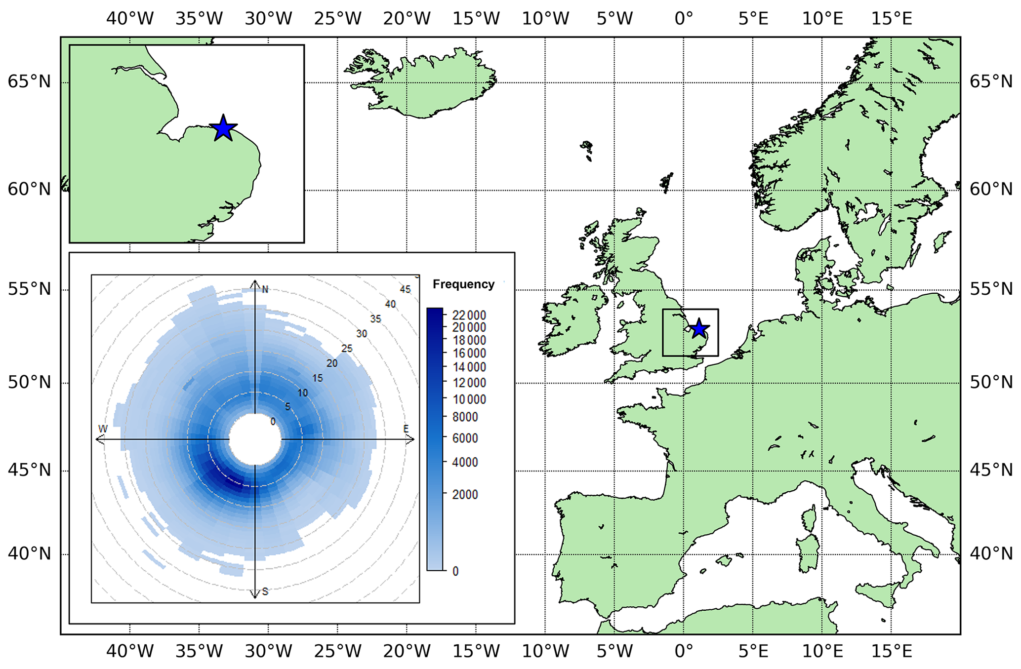
Figure 1 Map showing the location of the Weybourne Atmospheric Observatory (WAO, 52.95^∘ N, 1.12^∘ E) as a blue star. Bottom left inset: polar frequency plot showing wind speed (m s⁻¹) and wind direction at WAO averaged over the period 2016–2021. The frequency is the number of points with that wind speed and wind direction.

In the remainder of this paper, Sect. 2 describes the measurement system and the seasonal decomposition methodologies, and Sect. 3 provides an assessment of the measurement system's performance via intercomparison programme results, and repeatability and compatibility measures. In Sect. 4, we present the main features of the dataset: long-term trends, seasonal cycles, and diurnal cycles of CO₂, O₂ and APO. This analysis builds on work previously presented in the PhD theses of Wilson (2012) and Barningham (2018).

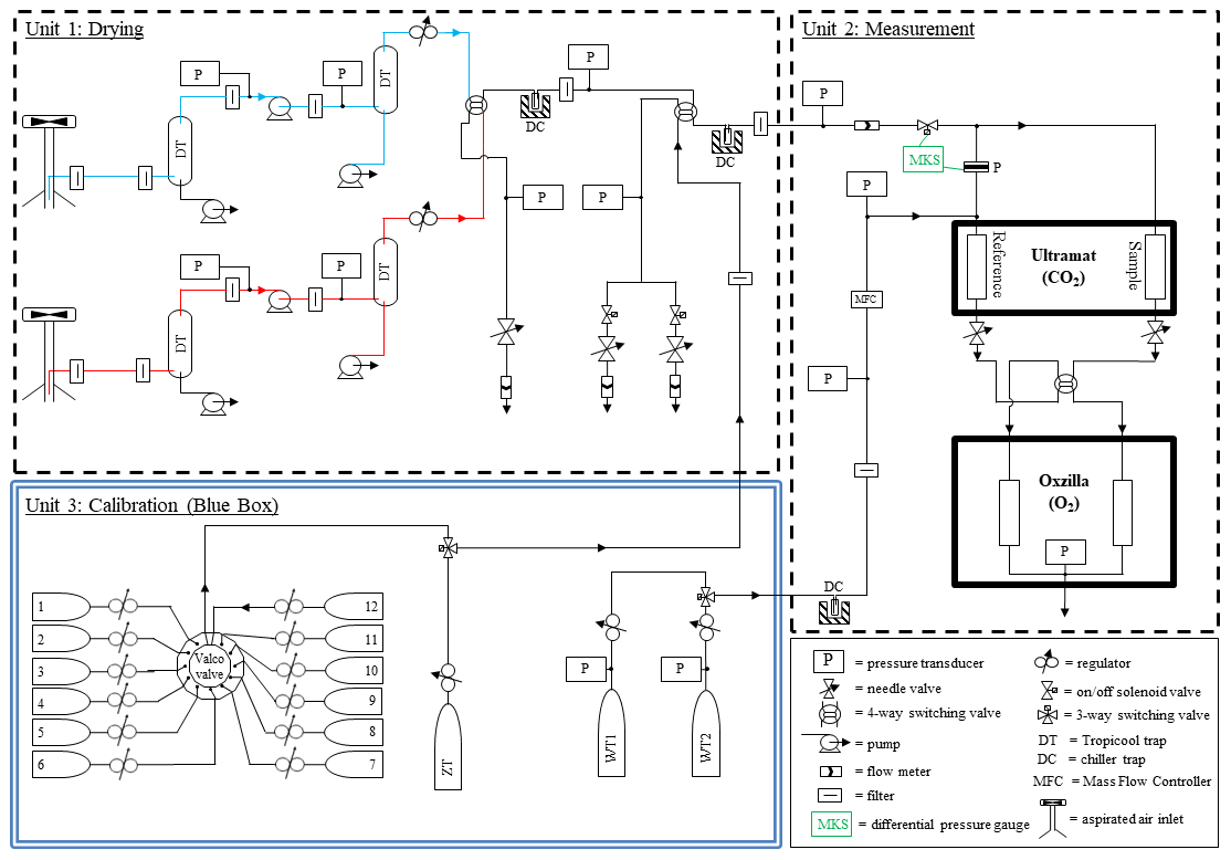
Figure 2 Gas handling diagram of the Weybourne Atmospheric Observatory (WAO) O₂ and CO₂ measurement system. The drying, measurement, and calibration units are shown in separate boxes. The “red” and “blue” inlet lines are coloured accordingly, and the green colouring denotes the “MKS” differential pressure gauge. The cylinders numbered 1–12 in the “Blue Box” demonstrate the maximum capacity of the multi-position “Valco” valve; these normally comprise of calibration cylinders, cylinders that are periodically measured as part of intercomparison programmes, Target Tanks (TTs), Zero Tanks (ZTs) and Working Tanks (WTs); see main text for details.

2 Methods

2.1 Analytical setup

The CO₂ and O₂ measurement system used at WAO is similar to those described in Stephens et al. (2007), Thompson et al. (2007) and Pickers et al. (2017). The WAO measurement system was first described in Patecki and Manning (2007) before it was deployed at WAO; it was also described in Pickers et al. (2022) and in the PhD theses of Wilson (2012) and Barningham (2018). There have been many modifications and upgrades to the system since it was first installed. The following description and Fig. 2 present the system as it stands in 2023.

There are two inlet lines, and the measurement system alternates sampling air between these two inlet lines every 2 h to diagnose for leaks, blockages, or other faults. The inlet lines are approximately 14 m long and are made of Synflex type 1300 tubing with an outer diameter of $\mathrm{1}/{\mathrm{4}}^{\prime \prime }$. Each inlet line includes an aspirated air inlet (Aspirated Radiation Shield Model No. 43502, Read Scientific Ltd.), whereby the inlet samples from a moving airstream and shields the entrance from solar radiation, to avoid fractionation of O₂ molecules relative to N₂ (Blaine et al., 2006) and a small diaphragm pump (KNF Neuberger Inc.; model PM27653-N86ATE) to draw air through the inlet tubing at 100 mL min⁻¹.

Air from the inlets passes through a two-stage drying system to dry the sample air to <1 ppm water vapour, which prevents dilution effects caused by water vapour that would otherwise bias the O₂ measurements (Stephens et al., 2007). The first stage of the drying system is a Peltier element thermo-electric cooler (Tropicool, model XC3000A), set at approximately 1 ^∘C. Water condenses out of the air and is drained away by peristaltic pumps (Cole Parmer, Masterflex). The Tropicool consists of stainless-steel traps filled with 4 mm diameter Pyrex glass beads (to provide greater surface area to promote water condensation). Traps are positioned both upstream and downstream of the diaphragm pump; the downstream pump provides better water condensation because of the above ambient pressure provided by the pump (∼3 bar), whereas the upstream pump prevents water build up in the pump itself. The second stage of the drying system is a VT490D cryogenic cooler (SP Scientific), which contains traps filled with 4 mm diameter Pyrex glass beads in a 4 L ethanol bath, and achieves a dew point of approximately −80 ^∘C.

The CO₂ mole fraction is measured by a non-dispersive infrared (NDIR) CO₂ analyser from Siemens Corp., model Ultramat 6E and the O₂ mole fraction is measured by an “Oxzilla”, a dual fuel cell O₂ analyser from Sable Systems International Inc. The fuel cells contain a gas-permeable membrane across which O₂ from the air permeates and undergoes electrochemical reduction in the cells, which contain a lead anode in an acidic electrolyte solution. The Ultramat and Oxzilla analysers are both differential analysers and are placed in series. Sample air flows through one side of the analysers, and air from the Working Tank (WT, see Sect. 2.2) flows continuously through the other side of the analysers; air from calibration, quality control and intercomparison cylinders passes through the “sample” side. The flow rate of the measurement system (both the sample and working reference sides) is set to 100 mL min⁻¹ using a mass flow controller (MFC, Fig. 2). The pressures and flow rates are carefully balanced to be the same on both the sample air and WT air sides of the analysers. This balance is achieved with a differential pressure transducer (MKS Instruments, model Baratron 223B), which measures the pressure difference between the sample and WT air streams and then adjusts the sample side pressure to match the pressure of the WT air using a fast-response solenoid valve (MKS Instruments Inc., 248A; Fig. 2).

A four-way switching solenoid valve (Numatics, model TM series) immediately upstream of the Oxzilla switches the sample air and WT air between each of the fuel cells every 60 s. Switching between sample air and WT air helps to eliminate short-term drift and increases the signal to noise ratio, since the amplitude of the fuel cell difference is doubled, but the noise remains the same (Stephens et al., 2007). The first 30 s of data after every switch are discarded. Using the remaining 30 s of data, the difference between the fuel cells is calculated. We refer to the fuel cell difference as the “double differential O₂ value”, and it is effectively twice the O₂ mole fraction (Stephens et al., 2007). The measurement system reports an O₂ and CO₂ measurement every 2 min.

As shown in Fig. 2, the measurement system includes several pressure transducers, flow metres, solenoid valves, a flow controller, and temperature sensors (not shown in Fig. 2) that are all connected to an electronics control box (custom built in-house). Bespoke software (custom built in-house) enables the automation of many of the routine processes and minimises human intervention. The software's automation functionality includes: measuring cylinders at predetermined intervals; switching between the two inlet sample lines; flushing sample or cylinder air prior to analysis, processing analyser signals to calculate calibrated mole fractions in near real-time; rejecting calibrations outside a set range and notifying the user when key diagnostics stray outside of acceptable ranges. The software also records all of the analyser and diagnostic data (i.e. pressure, flow and temperature data) and routinely backs up all data files. In addition, the system can be accessed and controlled remotely, with the software displaying most of the data in near real-time.

2.2 Calibration procedures

The measurement system includes a calibration unit, consisting of a thermally insulated housing for gas cylinder stabilisation, a so-called “Blue Box”, where high-pressure cylinders are stored horizontally, a requirement for high-precision O₂ measurements (Keeling et al., 2007) that minimises thermal and gravitational fractionation of O₂ and N₂ molecules inside the cylinders. Our calibration procedures are similar to those detailed for O₂ and CO₂ in Kozlova and Manning (2009). Stored in the “Blue Box” are Working Tanks (WTs), Working Secondary Standards (WSSs), Zero Tanks (ZTs) and Target Tanks (TTs), and occasionally cylinders that are part of intercomparison programmes.

A cylinder containing dry, compressed air, known as a Working Tank (WT), is continuously run through the reference side of the differential Ultramat and Oxzilla analysers. CO₂ and O₂ are measured by comparing the CO₂ and O₂ in the air from the inlets (i.e. the sample side) to the CO₂ and O₂ in the air from the WT. By measuring the difference, any analyser response variability independent of the atmospheric mole fractions, for example from changes in room temperature or atmospheric pressure, is largely mitigated, since these changes will affect both the inlet air and WT air to roughly the same degree (Stephens et al., 2007).

A suite of three Working Secondary Standards (WSSs), which have high, medium, and low mole fractions of O₂ and CO₂ spanning the typical range of mole fractions observed at the station, is used to calibrate the analysers every 47 h (see calibration scale information below). The Ultramat exhibits a non-linear response to CO₂, so a quadratic equation ($y=a{x}^{\mathrm{2}}+bx+c$) is used in order to appropriately fit the analyser response function. The Oxzilla exhibits a linear response, so a linear equation is used ($y=bx+c$). With the exception of the CO₂ c-term, the calibration coefficients are redetermined every 47 h, and then these new values are used until the next calibration.

The CO₂ c-term (sometimes called the zero coefficient) is redetermined every 3 or 4 h using a Zero Tank (ZT), which is a cylinder filled with ambient air, and is run immediately after every calibration and then every 3 or 4 h afterwards. This CO₂ c-term adjustment is done to correct for baseline response drift in the Ultramat analyser, which is predominately due to room temperature fluctuations in-between calibrations. The ZT correction is only required for the CO₂ measurements, as the double differential switching accounts for analogous short-term temperature related drift in the O₂ analyser. A Target Tank (TT), also filled with ambient air, is typically measured every 11 h as a quality control check on both the measurement system and the calibration procedures.

All cylinders used are 40 or 50 L high-pressure aluminium cylinders (Luxfer Gas Cylinders Inc.) filled with very dry air (<1 ppm water vapour content) to ∼200 bar, at the Cylinder Filling Facility (CFF) at the UEA before being deployed at WAO. The O₂ and CO₂ mole fractions in the WSSs and the TT are pre-determined at UEA's Carbon Related Atmospheric Measurement (CRAM) Laboratory, by measuring the cylinders using a bespoke Vacuum Ultraviolet (VUV) absorption analyser (Stephens et al., 2003) for O₂ and a Siemens Ultramat 6F analyser for CO₂, against a suite of primary standards obtained from NOAA (National Oceanic and Atmospheric Administration), USA and Scripps Institution of Oceanography (SIO) (see calibration scale information below). The WSSs and TTs are used at WAO until the cylinder pressure is ∼30 bar, and the WTs and ZTs are used until the cylinder pressure is ∼5 bar, as there is frequently outgassing of gases from cylinder walls at low cylinder pressures.

From its inception to June 2014, the WAO CO₂ data were reported on the SIO CO₂ calibration scale. From July 2014 to December 2021 the CO₂ data were reported on the WMO CO₂ X2007 scale. Presently, all the data from October 2007 to December 2021 have been transferred onto the WMO CO₂ X2019 scale using Eq. (6) in Hall et al. (2021). The WMO CO₂ X2019 calibration scale is maintained by the Central Calibration Laboratory (CCL) at the NOAA Earth System Research Laboratories (ESRL) Global Monitoring Laboratory (GML). The O₂ measurements are reported on the SIO “S2” scale that was used by SIO from April 1995 to August 2017 (Keeling et al., 2020). For O₂ measurements there is no formally recognised scale but most laboratories within the global O₂ community use or are linked to the SIO scale.

The measurement system was first installed at WAO in October 2007; however, between October 2007 and May 2010, the system was still being developed and underwent major changes, leading to large gaps in the dataset and much of the data being of unknown quality and with calibration scale issues. Therefore the data from this period have been excluded, and only data from May 2010 to December 2021 are publicly available and are discussed in this paper.

2.3 Seasonal decomposition

The baselines of all three species were calculated from the hourly averages with the Robust Extraction of Baseline Signal (REBS) method using the RFBaseline function within the IDPMisc package in R (Ruckstuhl et al., 2012; 2020). The RFBaseline function has three adjustable parameters: span, bi-weight function (b), and the number of iterations (maxit). The span is the smoothing time period, based on the frequency of data points. We have used a value of 0.01, which applies a smoothing window with a period of approximately 4 weeks, which we think is the most appropriate for distinguishing regional and background variability. The bi-weight function uses asymmetrical weighting, which is appropriate for CO₂ and O₂, where short-term excursions from the baseline are mostly uni-directional (positive for CO₂; negative for O₂); here, we used 0.01, and the number of iterations used is (4,0).

The time series were decomposed using the REBS results and STL (Seasonal Trend decomposition using LOESS (locally weighted scatterplot smoothing); Cleveland et al., 1990), so that salient features in long-term trends and seasonality can be described and quantified. The STL function (in R) performs a moving average calculation to separate the trend, seasonal and random components of the time series. STL has two smoothing parameters: s.window, which is the number of years to use when estimating the seasonal component, and t.window, which is the number of consecutive observations to use when estimating the trend. We used an s.window of 5 years (this value is often used in other studies (Pickers and Manning, 2015)) and a t.window of 13 149. Cleveland et al. (1990) suggests that the t.window should be approximately 1.5 to 2 times the number of observations in each year, for hourly data, that is 8766 h per year ($\mathrm{365.25}\cdot \mathrm{24}=\mathrm{8766}$), and $\mathrm{1.5}\cdot \mathrm{8766}=\mathrm{13}\mathrm{149}$. The decomposed time series are shown in the Supplement (Figs. S2–S4).

Since the currently available version of STL cannot handle gaps in the time series, the REBS results were interpolated using the na_seadec function in the imputeTS package in R (algorithm = “interpolation”, option = “spline”), prior to decomposition using STL. Gap filling is to take account of times when sample air is not being measured because of routine cylinder analyses, because of scheduled system maintenance, or because of inadvertent downtimes owing to system faults. Figure S1 shows the baseline data with the interpolated values. In order to avoid possible end effects with the STL decomposition (Pickers and Manning, 2015), the time series were extended by a year both forwards and backwards in time, by taking the interpolated data for the first year and the last year and adding and subtracting the average annual trends for each species (CO₂: 2.31 ppm yr⁻¹, O₂: −24.1 per meg yr⁻¹, APO: −12.0 per meg yr⁻¹). These average annual trends were from an initial run of STL. After the seasonal decompositions were completed, these extended years were removed for all subsequent analyses (including recomputing average annual trends). The baselines, the interpolation of the datasets, and the seasonal decompositions presented here are just one example of the methods and parameters that could be used, since time series decomposition can be susceptible to the choice of method and parameters (Pickers and Manning, 2015).

3 Repeatability and compatibility of the measurement system

The WMO/GAW sets compatibility goals for measurements of greenhouse gas and related species in the atmosphere based on what compatibility is scientifically desirable. Compatibility is a measure of the persistent bias between measurement records (Crotwell et al., 2020). These WMO compatibility goals are ±0.1 ppm for CO₂ in the Northern Hemisphere and ±2 per meg for O₂ globally. However, given current analytical capabilities, the O₂ goal is considered somewhat aspirational, as it is not routinely achievable. The WMO also provide an extended compatibility goal of ±10 per meg for studies where greater accuracy is not required (Crotwell et al., 2020), and which is routinely achievable for some laboratories. Nevertheless, for most applications of O₂ data from our WAO station, the extended compatibility goal is not sufficient, so we strive to get as close to the ±2 per meg goal as we can. We can also quantify repeatability from our datasets. Repeatability is a measure of the closeness of the agreement between the results of successive measurements over a short period of time (Crotwell et al., 2020). Repeatability goals should be one half of the network compatibility goals, that is, ±0.05 ppm for CO₂, and ±1 per meg for O₂ (or ±5 per meg for the extended O₂ goal). We have several ways in which to quantify compatibility and repeatability from our WAO datasets, which we discuss in this section, including results from intercomparison programmes, analysing data from our TT, ZT, and WT measurements, and examining the standard deviation of sample air data.

3.1 Intercomparison programmes

WAO has participated in three intercomparison programmes in order to assess the compatibility of WAO with other measurement sites. These intercomparison programmes are: “Cucumbers” (http://www.cucumbers.uea.ac.uk, last access: 17 November 2023); “GOLLUM” (Global Oxygen Laboratories Link Ultra-precise Measurements, http://www.gollum.uea.ac.uk, last access: 17 November 2023); and the WMO/IAEA Round Robin Comparison Experiment (World Meteorological Organization/International Atomic Energy Agency, http://gml.noaa.gov/ccgg/wmorr/index.html, last access: 17 November 2023). These intercomparison programmes involve measuring the same high pressure cylinders filled with dry air, circulated amongst different laboratories and field stations, and comparing the measurements. Each programme includes several trios of cylinders circulating amongst participants, except for the most recent WMO round (“Round 6”), where pairs of cylinders were circulated. The intercomparison results from WAO are shown in Fig. 3 and are plotted as the values measured at WAO minus the values from the first time the cylinders were measured at the central laboratories: Max Planck Institute for Biogeochemistry (MPI-BGC) for the Cucumbers; SIO for the GOLLUMs; and for the WMOs the NOAA/ESRL/GML for CO₂ and the National Center for Atmospheric Research (NCAR), USA. for O₂.

The average offsets at WAO relative to the initial central laboratory analysis, for CO₂ and O₂, are shown in Table 1. The average offset for the GOLLUMs is within the WMO compatibility goal (±0.1 ppm) but the Cucumbers and WMOs average offsets are larger. The GOLLUMs and Cucumbers ±1σ standard deviations are slightly larger than ±0.1 ppm, which implies that the WAO CO₂ measurements are not of sufficiently high precision to have confidence in the average offset. The WMOs ±1σ standard deviation is less than ±0.1 ppm, suggesting that the WAO CO₂ measurements are offset from the NOAA CO₂ values, although this is based on only two sets of measurements (in 2010 and 2015). For the Cucumbers, 16 out of the 30 sites involved in the programme, had a ±1σ standard deviation $>\pm \mathrm{0.1}$ ppm (Manning et al., 2014). This demonstrates that, even for a gas such as CO₂, where measurement precision is routinely achievable to WMO requirements, maintaining such compatibility at field stations over the long-term is still challenging owing to other gas handling and calibration effects, such as leaks, drifting mole fractions within cylinders, and disturbances to the ambient environment, for instance room temperature control issues (Manning et al., 2014).

Table 1 The average offsets at WAO relative to the initial central laboratory analysis for the three intercomparison programmes WAO participated in. These average offsets are the average of the cylinder differences and the ±1σ standard deviation of the cylinder differences.

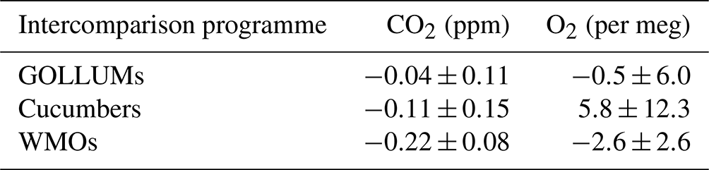
The WMO O₂ average offset is based on only one set of measurements of two cylinders (O₂ analysis was not an option with the WMO programme prior to Round 6). For Cucumbers none of the five sites measuring O₂ were within the ±2 per meg goal, and four of the five sites were within the ±10 per meg goal (Manning et al., 2014). The measurements made in 2015 have larger ±1σ standard deviations, since during this time the WAO O₂ analyser was performing less well (see Sect. 4.1). The GOLLUM cylinders tend to perform better than the Cucumber cylinders for O₂, possibly because Cucumbers was not specifically focused on O₂, and, therefore, the laboratories that were not doing O₂ measurements may not have treated the cylinders in the way that is typically used for O₂ measurements (e.g. vertical storage and non-ideal pressure regulators) and that this could have influenced the O₂ mole fraction in the cylinders. Some of the intercomparison cylinders had O₂ and CO₂ mole fractions outside of the calibration range of our measurement system, which may have influenced the results. The results of the intercomparison programmes should be kept in mind when comparing WAO data to other stations.

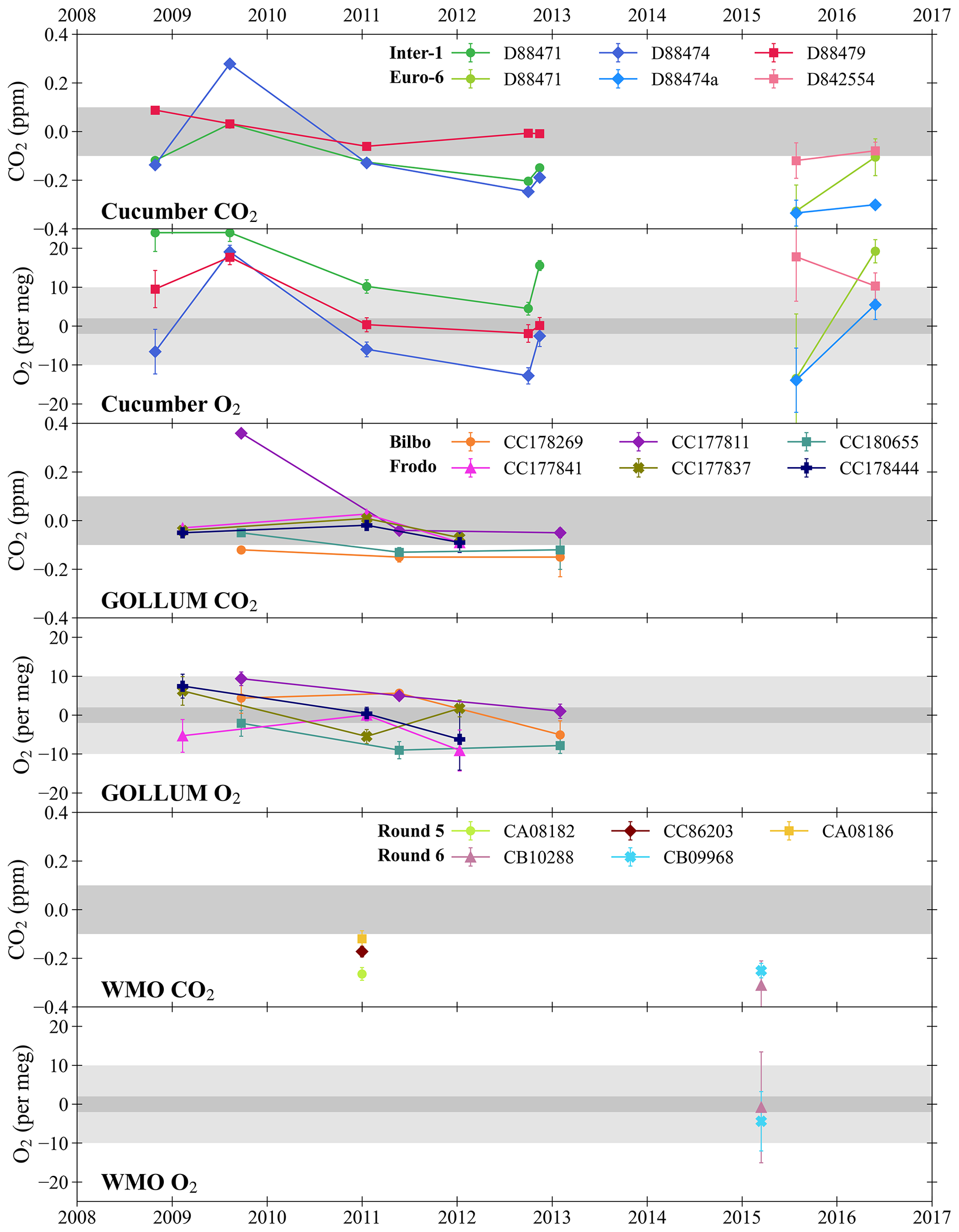
Figure 3 Cucumbers, GOLLUM, and WMO intercomparison cylinder results for CO₂ and O₂ plotted as the WAO measurements minus the initial central laboratory measurements. The horizontal shaded grey bands represent the WMO compatibility goals: ±0.1 ppm for CO₂, and ±2 per meg and ±10 per meg for O₂. The legends state the unique cylinder ID numbers. If the same cylinder was measured more than once throughout the programme, this is indicated by connecting symbols with lines. The error bars show the ±1σ standard deviation of the cylinder measurements and in some cases the error bars are smaller than the symbols. All programmes involve trios of cylinders, with the exception of “Round 6” of the WMO programme for which there were pairs of cylinders. WAO was originally part of the “Inter-1” Cucumbers rotation but later moved to the “Euro-6” rotation; WAO participated in both the “Frodo” and “Bilbo” GOLLUM rotations concurrently; and WAO participated in “Round 5” and “Round 6” of the WMO Round Robins. The x axis tick marks are at the beginning of each year.

3.2 Stability of Target Tank mole fractions

The Target Tank (TT) is used to check the performance of the O₂ and CO₂ measurement system and is typically measured every 11 h. The TT has a dual purpose: firstly, it is used to check how compatible the measurements at WAO are to the UEA CRAM Laboratory, where TT cylinders are usually analysed before being used at WAO. Secondly, the TT can also indicate the repeatability of the WAO CO₂ and O₂ analysers. Between May 2010 and December 2021, 11 TTs were measured at WAO, with a total of 8365 TT measurements, where we define a TT measurement as the mean of seven consecutive 2 min measurements. TT measurements made when there were known technical issues have been removed, resulting in 961 O₂ and 878 CO₂ TT measurements removed, leaving 89 % of the O₂ data and 90 % of the CO₂ data. The TT does not pass through the inlet lines or the first stage of the drying system (Fig. 2), and, therefore, the repeatability of the TT measurements is not a quality control check on the whole measurement system but of the analysers, the internal calibration, and the gas handling system from the TT to the analysers.

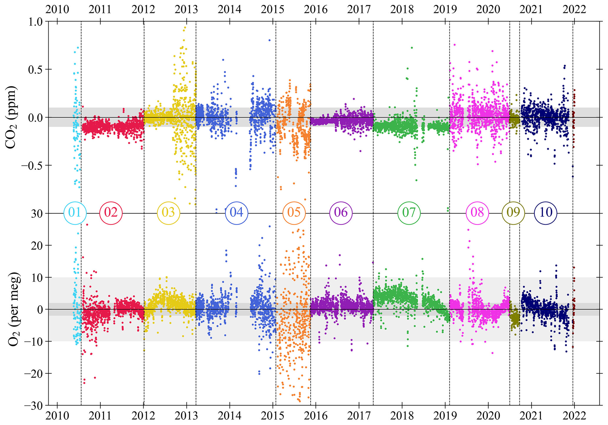
Figure 4 Target Tank (TT) measurements of CO₂ (top panel) and O₂ (bottom panel) at WAO between May 2010 and December 2021. Data are plotted as the difference from the UEA CRAM Laboratory “declared” values (measured minus declared), with each cylinder plotted in a different colour and separated by vertical dashed lines. Cylinders are numbered in the order that they were used. Each TT measurement shown is the mean of seven consecutive 2 min measurements of O₂ and CO₂. Note that 10 and 18 measurements are off scale in the O₂ and CO₂ panels, respectively, out of more than 7000 measurements shown for each species. The O₂ y axis is not visually comparable on a mole per mole basis to the CO₂ y axis. Horizontal black lines are at zero difference, and the horizontal shaded grey bands represent the WMO compatibility goals: ±0.1 ppm for CO₂, ±2 per meg and ±10 per meg for O₂.

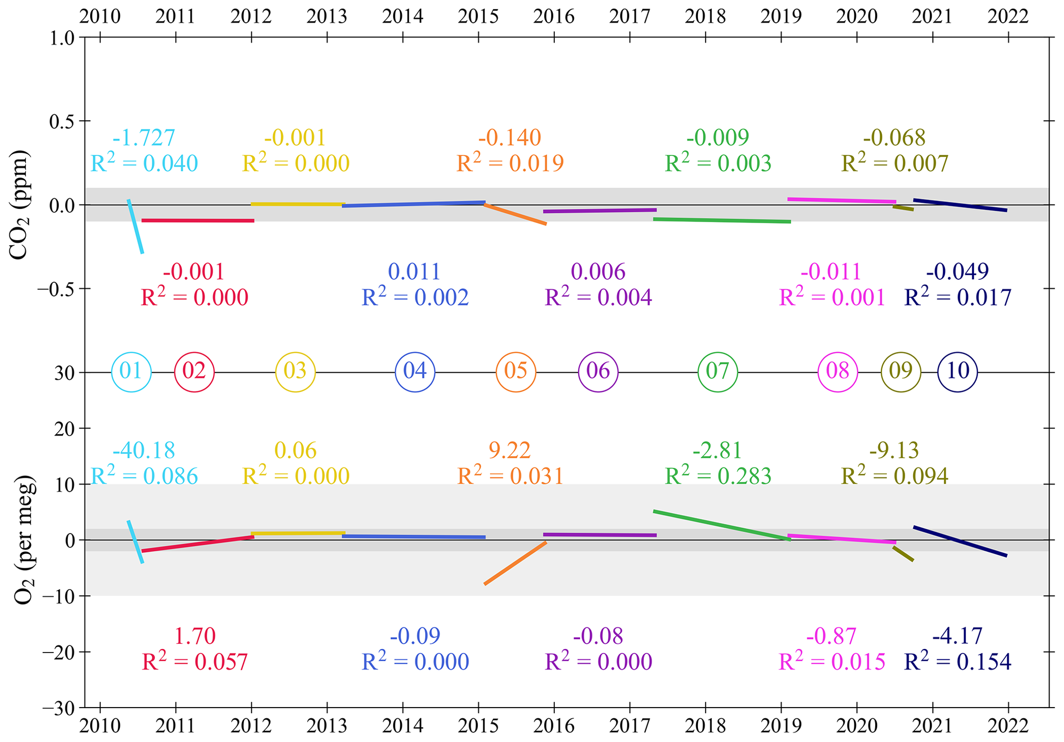
Figure 5 Linear trend lines for each Target Tank (TT), with slopes (in ppm yr⁻¹ and per meg yr⁻¹, for CO₂ and O₂, respectively) and R² of the Pearson correlation reported for each TT, for CO₂ (top panel) and O₂ (bottom panel) at WAO between May 2010 and December 2021. As in Fig. 4, cylinders are numbered in the order that they were used, horizontal black lines are at zero difference between WAO and UEA, and the horizontal shaded grey bands represent the WMO compatibility goals: ±0.1 ppm for CO₂, ±2 per meg and ±10 per meg for O₂. The 11th TT is not shown as the time period that it was in use is too short for meaningful results.

The CO₂ and O₂ TT results as differences from the UEA CRAM Laboratory declared values are shown in Fig. 4, and in Fig. 5, for each TT cylinder, we show the linear trend lines of the TT differences with their slope and Pearson correlation (R²). Ideally, both the slope of the linear trend line and the R² for each cylinder would be zero. Anything other than zero could indicate a drift in the calibration scales defined by the measurement system at WAO or a drift in the mole fractions in the TT itself.

The WAO CO₂ measurements for TT02 and TT07 are both approximately 0.1 ppm lower than the UEA CRAM Laboratory declared values (Fig. 5). For CO₂ TT01 and TT05 both have decreasing trends (Fig. 5); however, these TTs exhibited more variable measurements than the other TTs (Fig. 4), so it is possible that these trends are not robust. All the TTs, except TT01, have linear trend lines with slopes that are less than ±0.15 ppm yr⁻¹ and R²<0.02, suggesting that there is no significant drift in CO₂ mole fractions. In September 2012 the TT CO₂ measurements were more variable due to decreased performance of the CO₂ analyser (Fig. 4).

For O₂, there are five cylinders that have a slope greater than ±2 per meg yr⁻¹ (Fig. 5). TT01 has a decreasing trend, and TT05 has an increasing trend; however, these TTs exhibited more variable measurements than the other TTs (Fig. 4), which may have influenced the perceived drifts in their values, and they both have R²<0.09. TT01 is a 20 L cylinder (all other TTs are between 40–50 L), and there is evidence that smaller cylinders have less stable mole fractions (Pickers, 2016), and this cylinder was used, with no conditioning, immediately after it had been evacuated. TT05 was the TT being used in 2015 when the Oxzilla precision was poor. TT01 and TT05 are also the cylinders with the poorest compatibility and repeatability, excluding the final cylinder (Table 2). There are three remaining cylinders that show evidence of drift and have R²>0.09. TT09 and TT10 both have decreasing O₂ mole fractions during the whole of their run, whereas TT07 O₂ mole fractions only start decreasing during the last 4 months of its run (Fig. 4). For these three cylinders the Zero Tank (ZT) O₂ measurements for the same time periods were investigated (see Sect. 3.3). The ZT is used to adjust the CO₂ calibration c-term, but O₂ is also measured during these runs, because the analysers are connected in series. Therefore, if the ZT O₂ is also drifting then that would indicate that the measurement calibration is drifting, whereas if it is not drifting that would indicate that it is the mole fraction in the TT itself which is drifting. For TT07, TT09, and TT10 the ZT O₂ mole fractions were not drifting at the same time, and, therefore, the drift is most likely caused by the TTs themselves.

Table 2 Repeatability and compatibility of the WAO O₂ and CO₂ measurement system indicated by the Target Tanks (TT). Note that we report air measurements between May 2010 and December 2021, so we investigated TT measurements for the same time period; this means the first and last cylinders do not include the whole time period when they were used.

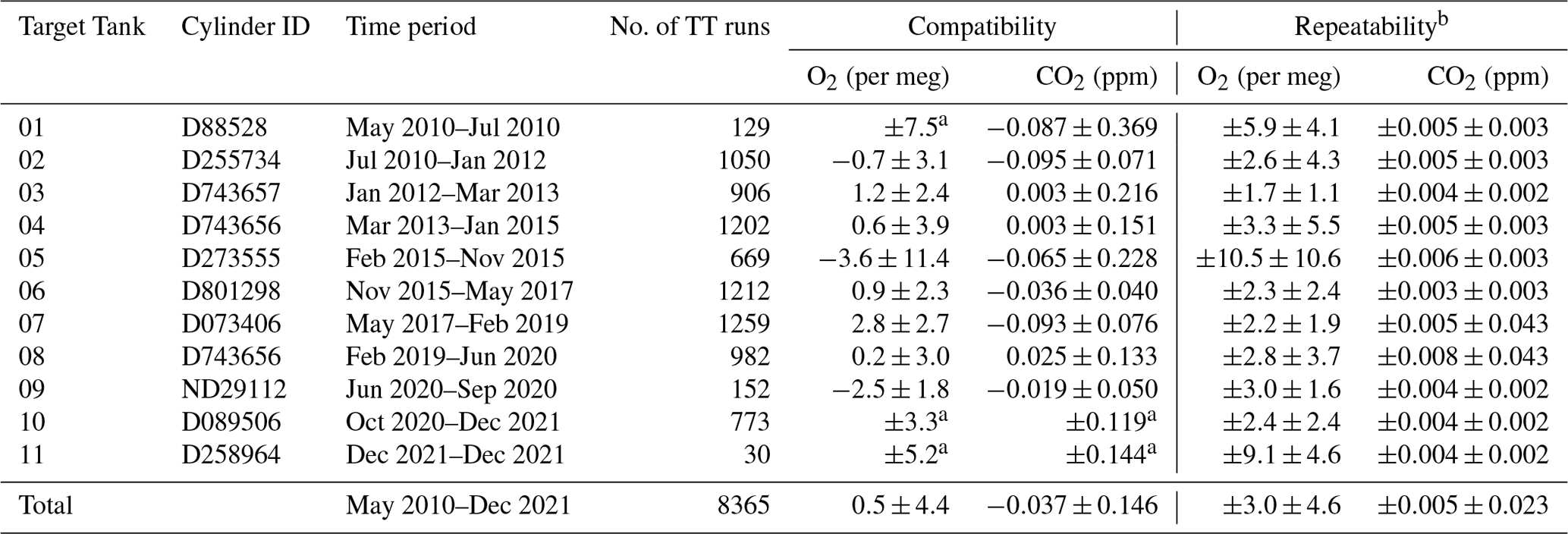
^a These cylinders were not measured at the UEA CRAM Laboratory, so the compatibility cannot be calculated, but the average of the WAO measurements was used to calculate ±1σ standard deviation for each cylinder. ^b Repeatability was calculated using the same method as Kozlova and Manning (2009) and Pickers et al. (2017), from the mean ±1σ standard deviations of the average of two consecutive 2 min TT measurements. TT repeatability is reported with ±1σ uncertainty, which recognises the fact that the measurement system repeatability varies over time.

Table 2 shows the compatibility of the measurement system which is the average of the differences between the TT measured values and UEA CRAM Laboratory declared values and the ±1σ standard deviation. The UEA CRAM Laboratory calibration scales are traceable to the WMO CO₂ X2019 scale and the SIO O₂ scale (see Sect. 2.2). The overall compatibility for CO₂ is $-\mathrm{0.037}\pm \mathrm{0.146}$ ppm, which is within the WMO compatibility goal (±0.1 ppm), although the ±1σ standard deviation is slightly larger than the compatibility goal. The TT CO₂ compatibility is $<\pm \mathrm{0.1}$ ppm for 67 % of the measurements. The overall compatibility for O₂ is 0.5±4.4 per meg, which is within the compatibility goal of ±2 per meg, although the ±1σ standard deviation is larger than the compatibility goal. The TT O₂ compatibility is $<\pm \mathrm{2}$ per meg for 54 %, $<\pm \mathrm{5}$ per meg for 87 % and $<\pm \mathrm{10}$ per meg for 96 % of the measurements. The average overall compatibility is smaller than the ±1σ standard deviation for both O₂ and CO₂, meaning that there is not a statistically significant difference between the WAO measurement system and the UEA CRAM Laboratory.

Table 2 shows the repeatability of the TTs for each cylinder. Each TT data point is the mean of seven consecutive 2 min averages. We calculate the mean of ±1σ standard deviations for every two consecutive 2 min averages for each TT run. This average of the ±1σ standard deviation for each TT run is then averaged together for each cylinder and for the whole time period to determine the repeatability. The TT repeatability is reported with the ±1σ standard deviations of the averages for each TT run. Ideally, the repeatability of a measurement system should be no more than half the compatibility goal, i.e. ±0.05 ppm for CO₂ and ±1 per meg/±5 per meg for O₂.

Overall, the repeatability of the measurement system was $\pm \mathrm{0.005}\pm \mathrm{0.023}$ ppm for CO₂, which is an order of magnitude smaller than the repeatability goal. For O₂ the overall repeatability was $\pm \mathrm{3.0}\pm \mathrm{4.6}$ per meg, which is greater than the ±1 per meg ideal repeatability goal but is within the extended repeatability goal of ±5 per meg. The CO₂ repeatability is smaller than the CO₂ compatibility, $-\mathrm{0.037}\pm \mathrm{0.146}$ ppm, whereas the O₂ repeatability is larger than the O₂ compatibility, 0.5±4.4 per meg, because O₂ repeatability is much more technically challenging than CO₂ repeatability. The ±1σ standard deviations for the O₂ repeatability and the O₂ compatibility are similar, ±4.6 per meg and ±4.4 per meg, respectively.

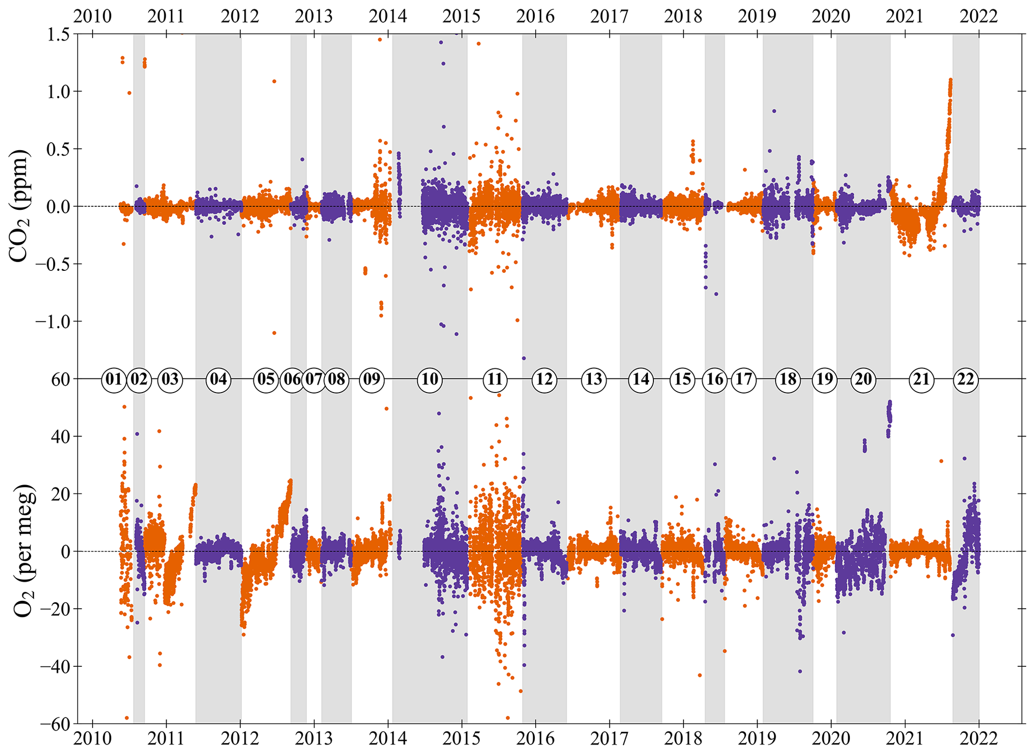
Figure 6 The CO₂ (top panel) and O₂ (bottom panel) Zero Tank (ZT) mole fractions as the difference from the average mole fraction (measurement minus average) for each ZT at WAO between May 2010 and December 2021. The ZTs alternate between orange and purple, and alternate shaded grey bands, to show when the ZT changes. On the y axes “zero” is the average mole fraction for each ZT. The O₂ y axis is not visually comparable on a mole per mole basis to the CO₂ y axis. Cylinders are numbered in the order that they were used. Note that seven and seven measurements are off scale in the O₂ and CO₂ panels, respectively, out of more than 20 000 measurements shown for each species.

3.3 Stability of Zero Tank mole fractions

The Zero Tanks (ZTs) are used to adjust the intercept of the CO₂ calibration curve in-between calibrations to correct for baseline drift in the CO₂ analyser response caused by changes in temperature (see Sect. 2.2). The O₂ in the ZT is also measured but is not used as part of the calibration. The ZT mole fractions are not measured at the UEA before being sent to WAO, and, therefore, the ZTs cannot be used to assess the compatibility of the WAO system with the UEA CRAM Laboratory. The ZTs can be used to access the O₂ and CO₂ repeatability of the measurement system in the same way as the TTs (see Sect. 3.2).

The ZT is typically measured every 3 to 4 h, and between May 2010 and December 2021 there were 26 359 ZT measurements. Measurements made when the system was experiencing known technical issues have been removed; this was 2672 measurements for CO₂ and 2866 measurements for O₂, leaving 90 % of the CO₂ ZT data and 88 % of the O₂ ZT data. The ZT mole fractions were between 354 ppm and 429 ppm for CO₂. Excluding ZT20, which had an O₂ value of 294 per meg, the ZT O₂ values ranged from −478 per meg to −1363 per meg.

The O₂ and CO₂ ZT mole fractions are shown in Fig. 6 as the difference from the average mole fraction of each cylinder. Table 3 shows the average ZT repeatability calculated in the same way as the TT repeatability (see Sect. 3.2) and the drift in the ZT O₂ mole fractions over time. We can see that there were time periods when the system was more stable and when it was less stable. This, in general, is similar to the TTs; for example, the ZTs also show that 2015 had very noisy oxygen measurements due to poor Oxzilla performance.

ZT03, ZT05, and ZT22 have O₂ mole fractions that drift upwards over time because they were not always stored horizontally (Fig. 6). ZT03 was originally positioned horizontally but then in December 2010 it was moved out of the Blue Box and was positioned vertically, to make space for other cylinders, and this caused the ZT O₂ mole fractions to start drifting upwards. ZT05 was positioned vertically for the whole of its run, so its O₂ mole fractions are drifting upwards the whole time. ZT22 was originally positioned vertically and then in November 2021 it was put horizontally, which is why the measurements for ZT22 drift upwards at the beginning and then stop. The ZT O₂ measurement is not used in the calibration, so these drifts do not affect the measurement system performance. ZT02 has O₂ mole fractions that drift downwards over time. The TTs O₂ mole fractions were not drifting at the same time, so it is likely that the ZT itself was drifting, not the measurement system. ZT01 shows a decreasing O₂ linear trend line; however, during this time, the measurements were noisy, so we have low confidence in the slope of the trend.

The CO₂ mole fraction of ZT21 drifts upwards at the end because the internal walls of this cylinder were cleaned using “sand blasting”, and it was then measured at WAO to investigate what effect this would have on the stability of the O₂ and CO₂. It was found the CO₂ mole fractions in the cylinder drift upwards at lower pressures, but there was no noticeable effect on O₂. The ZT is used to recalibrate the intercept every 3 to 4 h, and the within-cylinder drift in this time period should be small enough to not affect the measurements. In order to be confident that there is no effect on the measurements, “sandblasted” cylinders should not be used as ZTs once the internal pressure drops below 15 bar.

If we exclude the three ZTs that were vertical, the average CO₂ and O₂ repeatability based on the ZTs is $\pm \mathrm{0.005}\pm \mathrm{0.019}$ ppm and $\pm \mathrm{3.1}\pm \mathrm{5.3}$ per meg, respectively, which is similar to the CO₂ and O₂ repeatability based on the TTs ($\pm \mathrm{0.005}\pm \mathrm{0.023}$ ppm and $\pm \mathrm{3.0}\pm \mathrm{4.6}$ per meg, see Sect. 3.2). These results increase our confidence that this is the repeatability of the measurement system.

Table 3 Repeatability of the Zero Tank (ZT) O₂ and CO₂ measurements at WAO. We have calculated the O₂ linear trend line for the time period each ZT was used and report here the slope and R² of the Pearson correlation. Note that we report air measurements between May 2010 and December 2021, so we investigated ZT measurements for the same time period, this means the first and last cylinders do not include the whole time period when they were used.

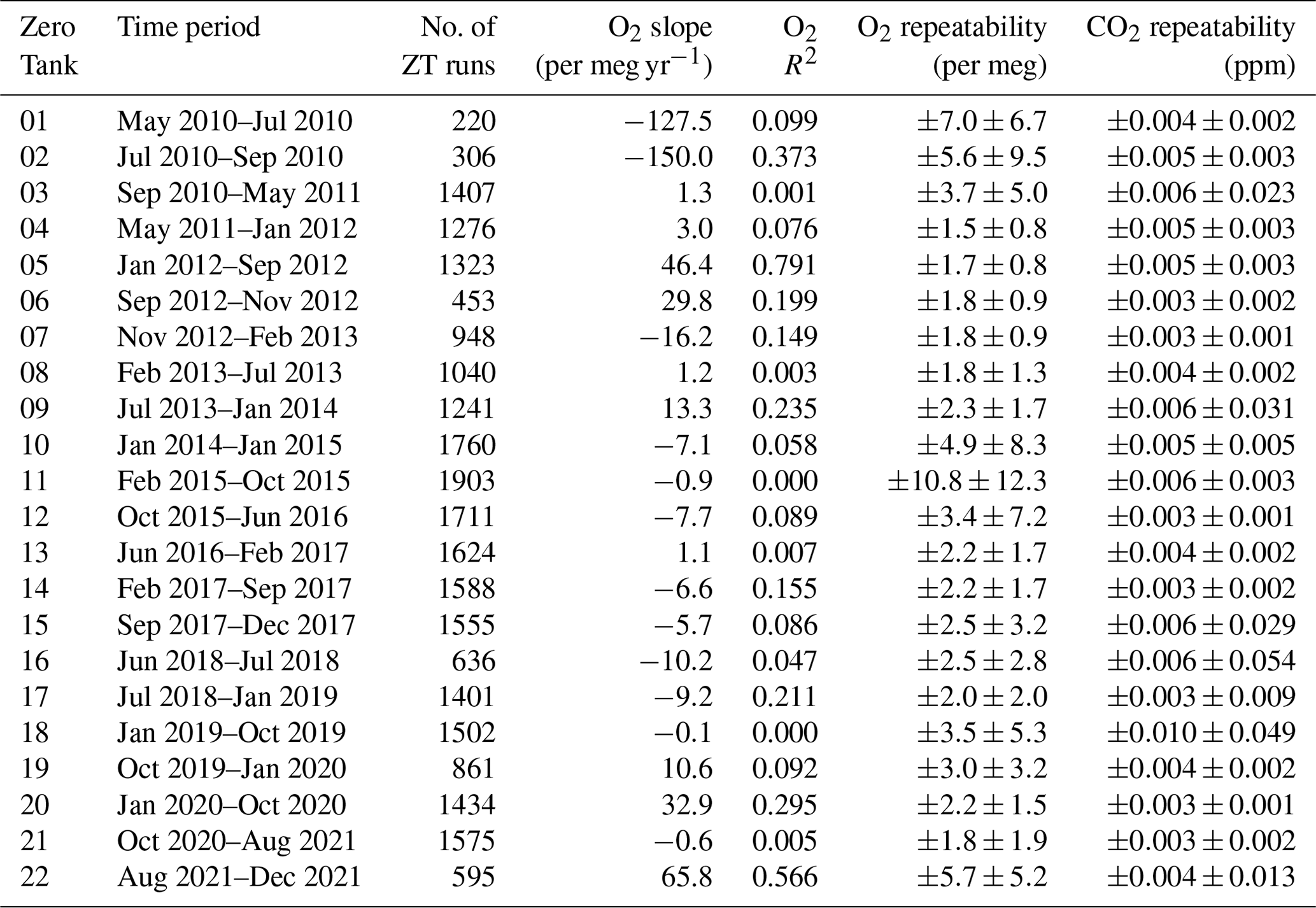
Figure 7 shows the absolute difference in the CO₂ mole fractions between the current ZT and the previous ZT (measured 3 to 4 h earlier). The ZT is used to adjust the intercept of the CO₂ calibration curve in-between calibrations, and it is assumed that the difference between the current ZT and the previous ZT is caused by drift in the baseline response of the CO₂ analyser. The average absolute difference in CO₂ is 0.03 ppm, which is less than the ±0.05 ppm repeatability goal, overall, 85 % of the differences are <0.05 ppm. These differences suggest that the ZT is measured regularly enough that the drift in the baseline is kept small enough to not substantially effect the measurements.

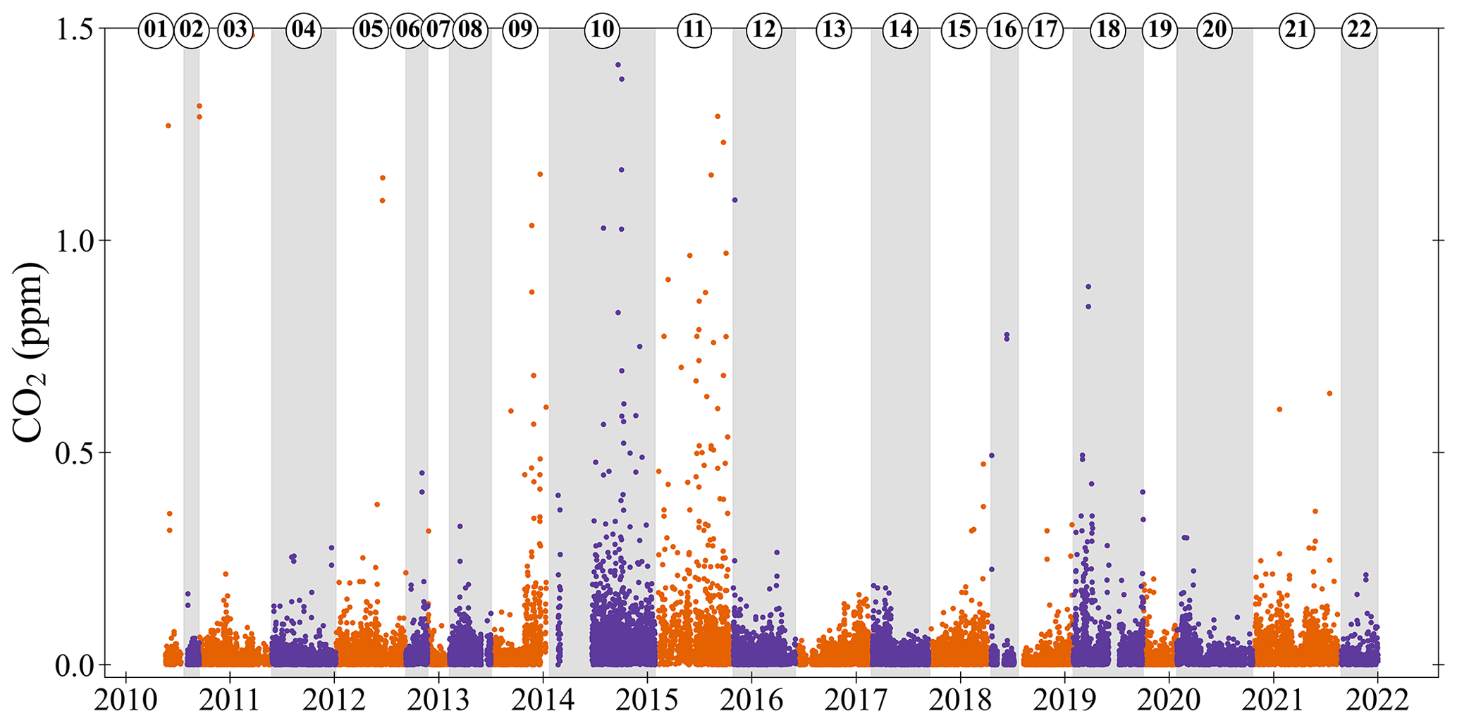
Figure 7 Absolute differences between the ZT CO₂ mole fraction and the previous ZT CO₂ mole fraction (current minus previous; typically measured 3 to 4 h earlier). As in Fig. 6, the orange and purple alternating colours, and shaded grey bands, show when the ZT changes, and cylinders are numbered in the order that they were used. Note that 13 measurements are off scale, out of more than 20 000 measurements shown.

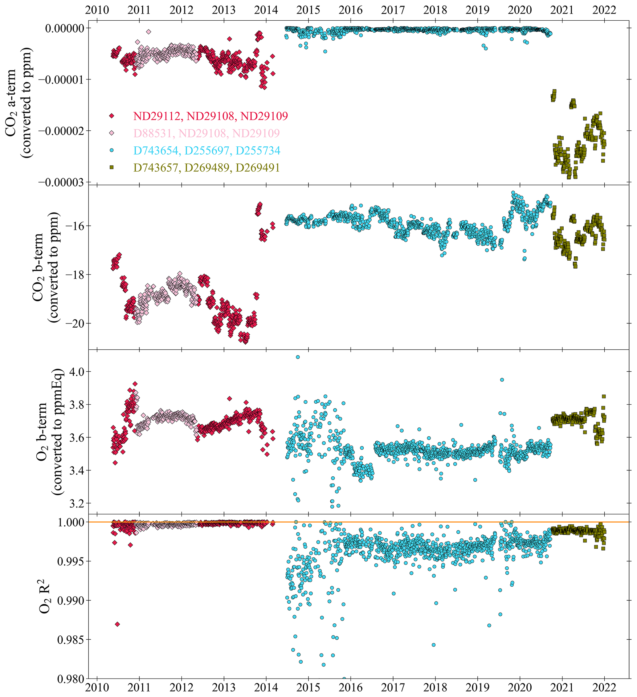
Figure 8 The CO₂ a and b terms, from the CO₂ calibration quadratic equation, $y=a{x}^{\mathrm{2}}+bx+c$, and the O₂ b-term and O₂ R², from the O₂ calibration linear equation, $y=bx+c$, of the WSS calibrations at WAO between May 2010 and December 2021. The colours and symbols indicate different WSS sets of cylinders and 1.0 on the O₂ R² panel is indicated by a horizontal orange line. The c-terms for each species, equivalent to the WT mole fractions, are shown in Fig. 10. Note that five measurements are off scale in the O₂ R² panel, out of more than 1700 measurements shown.

3.4 Stability of calibration coefficients

Three Working Secondary Standard (WSS) cylinders are used to calibrate the measurement system every 47 h (see Sect. 2.2). The c-terms of these equations are discussed in Sect. 3.5. In this section, we discuss the a-term and b-terms of the CO₂ and O₂ calibrations. We also discuss the Pearson correlation coefficient, R², of the measured O₂ mole fractions. Each of these parameters is shown in Fig. 8 as a time series. As three WSSs are used, and the CO₂ response is a quadratic equation, the CO₂ R² is always exactly 1.0. The Ultramat and Oxzilla report uncalibrated raw values of CO₂ and O₂ in units of vpm and %, respectively. The calibration coefficient units were converted from ppm vpm⁻¹ to ppm for CO₂ and ppmEq %⁻¹ to ppmEq for O₂. This conversion was done by multiplying the coefficients by the average analyser response of WSSs between June 2014 and September 2020: D255734 for CO₂ (399.37 ppm, −18.77 vpm) and D743654 for O₂ (−709.0 per meg, −122.7 ppmEq, 0.00072 %). At WAO between May 2010 and December 2021, three sets of WSS cylinders were used (Table 4). In total, there were 2038 calibrations; calibrations when the system was experiencing known technical issues were excluded, this was 277 for CO₂ and 293 for O₂, so this leaves 86 % of the data.

If the calibration coefficient terms drift over time, this could indicate a drift in the analyser sensitivity or a drift in the calibration scale. A drift in the sensitivity of the analyser may impact the precision and the accuracy. By calibrating frequently, the accuracy of the measurement should be less susceptible to drift in the analysers' sensitivity. However, a deterioration in the precision cannot be corrected for. A drift in the calibration scale may be caused by internal drift of the mole fractions in the calibration cylinders. This can only be determined by reanalysing the calibration cylinders after they have finished being measured at WAO. However, due to practical constraints this is not done on the calibration cylinders used at WAO. While we cannot know if the calibration cylinders have drifted over time, if they had drifted we would expect to see a noticeable step change in the air measurements when the calibration cylinders are changed and/or visible drift in the TT measurements (depending on the rate of the drift). In addition, we would expect to see evidence of long-term drift in our intercomparison programme results.

There are sometimes step changes in the calibration coefficients when the WSS cylinders are changed as the cylinders have different mole fractions in them. There are also sometimes step changes when the cylinders are not changed. These step changes are most likely caused by changes in the analyser response as it is very unlikely that the mole fractions in the cylinders would suddenly change very quickly and then stop. For example, the CO₂ b-term has a step change in October 2013, when the Ultramat analyser was changed.

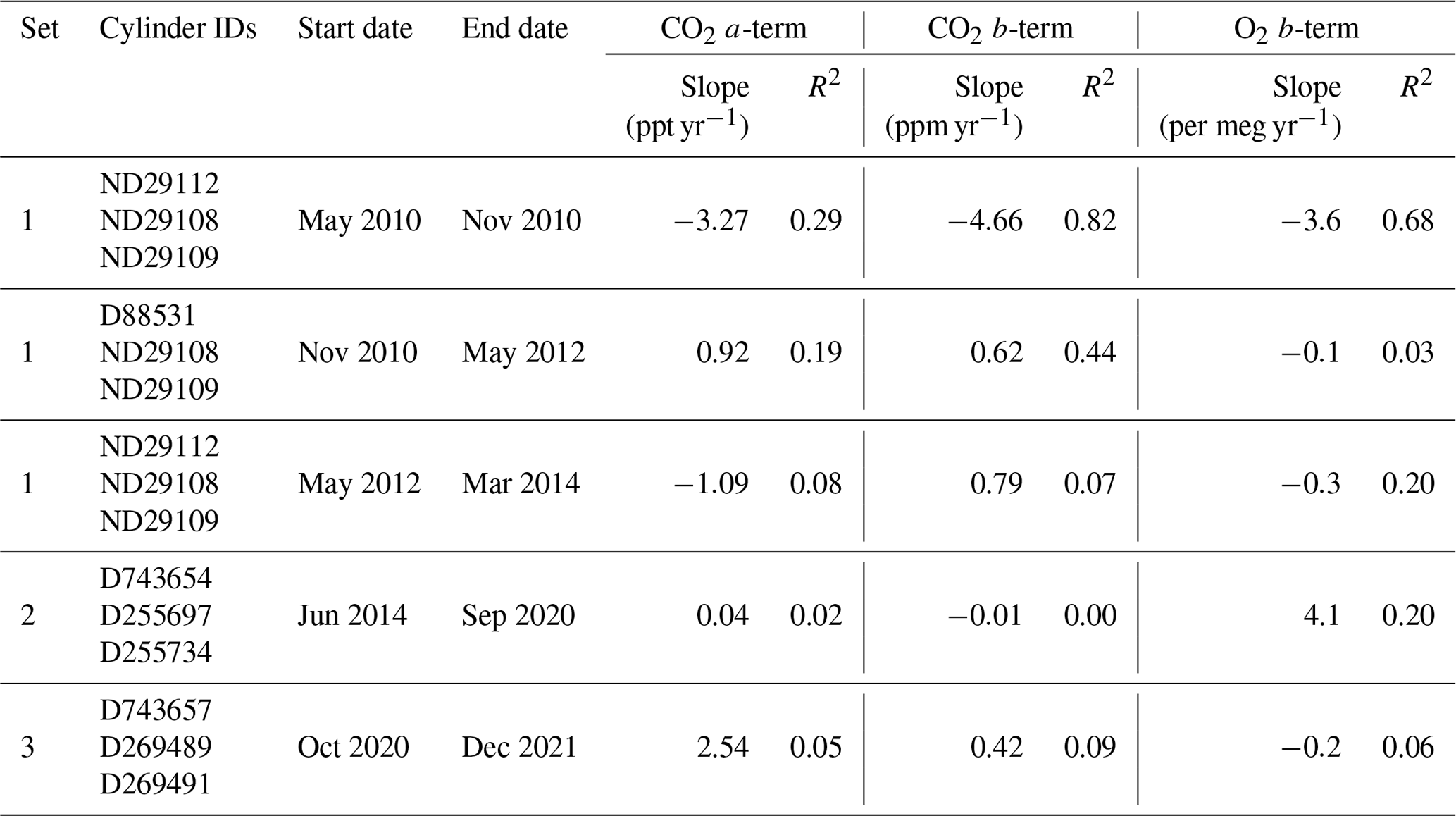
The drift in the calibration coefficients was calculated using the slope in the linear trend line for each of the five time periods WSSs were measured for (Table 4). The CO₂ a-term is small, and, therefore, the drift in the CO₂ a-term is also small, less than ±4 ppt yr⁻¹, indicating that the CO₂ analysers at WAO have a very linear response. There is a large drift between May 2010 and November 2010, the first time ND29112 (Set 1) was used, for both the CO₂ b-term (4.66 ppm yr⁻¹) and O₂ b-term (−3.6 per meg yr⁻¹). The smallest drift in the CO₂ b-term, −0.01 ppm yr⁻¹, occurs between June 2014 and September 2020 when Set 2 of the WSSs is used. For the O₂ b-term, three out of the five periods have drift that is less than ±0.3 per meg yr⁻¹. The largest drift in the O₂ b-term, 4.1 per meg yr⁻¹, occurs when Set 2 of the WSSs is used, but this is strongly influenced by the calibrations in 2014 and 2015 when there were issues with the measurement system. If the slope is recalculated starting from January 2016 instead, then the drift decreases to −1.9 per meg yr⁻¹. The O₂ and CO₂ mole fractions in the TTs and ZTs were not drifting at the same time (see Sect. 3.2 and 3.3), therefore indicating that it is not the cylinders that are drifting but the analyser sensitivity. The analyser sensitivity drifting should not affect the measurement results so long as the analyser response drift is not significant within a 47 h time period.

Table 4 All the cylinders that were used as WSSs at WAO. Three sets of WSS cylinders were used (Set 1: May 2010–March 2014, Set 2: June 2014–September 2020, Set 3: October 2020–December 2021). In November 2010, ND29112 was replaced with D88531, then in May 2012 was changed back to ND29112. For each calibration parameter, we report the slope and R² of the linear trend line. The slopes of the CO₂ a-terms are in units of ppt yr⁻¹ (parts per trillion per year). The slopes of the O₂ b-terms were multiplied by 6.05 to convert them from ppmEq yr⁻¹ to per meg yr⁻¹.

The O₂ R₂ varies over time. It is highest and most stable when Set 1 of the WSSs is being measured between 2010 and 2014; on average the O₂ R² during this time is 0.9997. In 2014 and 2015, there is additional evidence of the poorer performance of the Oxzilla analyser during this time, and the O₂ R² are smaller and much more variable. From 2016 to 2020 the O₂ R² is higher and more stable, although it is not as good as it was when Set 1 of the WSSs was being measured, on average the O₂ R² during this time is 0.9968. When Set 3 of the WSSs is being measured the O₂ R² is higher and more stable than it was with Set 2 but still not as good as it was with Set 1; on average for Set 3 the O₂ R₂ is 0.9988. Overall, from May 2010 to December 2021, the O₂ R² is on average 0.9977 and is >0.995, 92 % of the time.

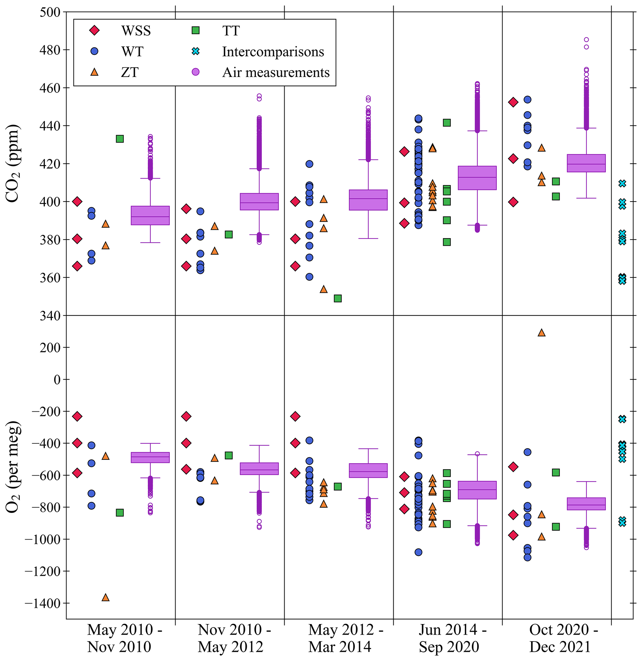
Figure 9 The CO₂ (top panel) and O₂ (bottom panel) mole fractions of the WSSs, WTs, ZTs, TTs, and intercomparison cylinders measured at WAO between May 2010 and December 2021. The air measurements made at WAO during this time are shown as box and whisker plots. The O₂ y axis is not visually comparable on a mole per mole basis to the CO₂ y axis.

The calibration range is between the WSS cylinder with the highest mole fraction and the WSS cylinder with the lowest mole fraction. It is intended that the calibration range is large enough to cover the range of mole fractions likely to be measured in the air at WAO. For CO₂, 77 % of the air measurements, 54 out of 73 WTs, 18 out of 22 ZTs, and 7 out of 11 TTs are within the calibration range (Fig. 9). For O₂, 74 % of the air measurements, 31 out of 73 WTs, 9 out of 22 ZTs, and 7 out of 11 TTs, are within the calibration range (Fig. 9). We can have less confidence in the accuracy of mole fractions measured outside the calibration range, and the further away from our calibration range the measurement is, the less confidence we can have. This is more the case for CO₂, for which the analyser has a non-linear response, than for O₂, which has a linear response.

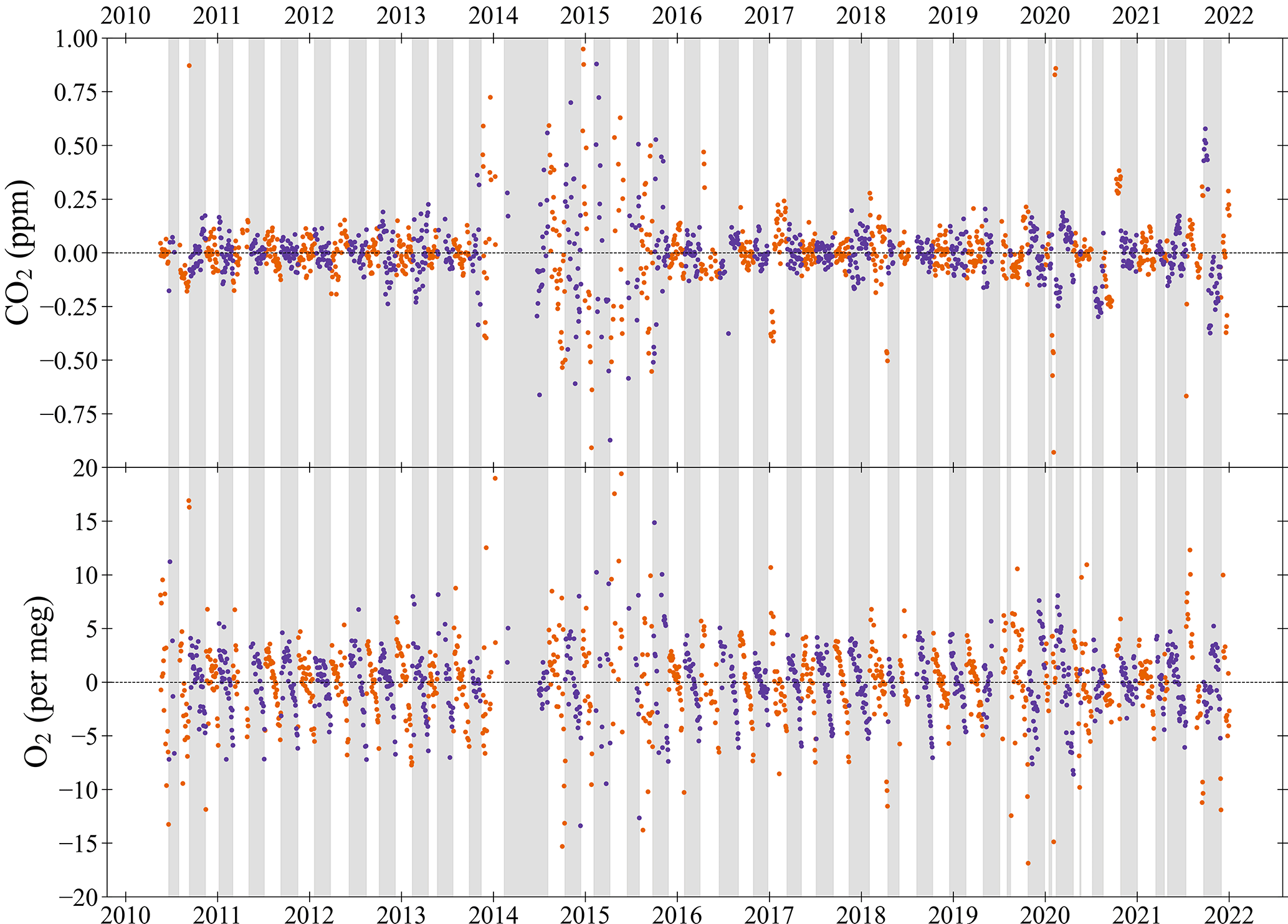
Figure 10 The CO₂ (top panel) and O₂ (bottom panel) Working Tank (WT) mole fractions calculated from the calibrations as the difference from the average mole fraction for each WT (measurement minus average) at WAO between May 2010 and December 2021. The WTs alternate between orange and purple, and alternate shaded grey bands, to show when the WT changes. On the y axes “zero” is the average mole fraction for each WT (dashed line). The O₂ y axis is not visually comparable on a mole per mole basis to the CO₂ y axis. Note that five and seven measurements are off scale in the O₂ and CO₂ panels, respectively, out of more than 1700 measurements shown for each species.

3.5 Stability of Working Tank mole fractions

Since all measurements are taken against the reference of the Working Tank (WT) this means that the intercept (i.e. the c-term) of the calibration curves for both CO₂ and O₂ is the WT mole fraction at the point of calibration. Calibrations typically take place every 47 h, and the stability of the WT mole fraction over time provides another measure of system performance. Usually, WTs are 50 L cylinders filled to ∼200 bar, which are used until their pressure gets below ∼5 bar. The measurement system flow rate is approximately 100 mL min⁻¹, and on average WTs last 55 d. Between May 2010 and December 2021, 76 Working Tanks were measured at WAO. In total there were 2038 calibrations between May 2010 and December 2021. Calibrations made when the system was experiencing known technical issues have been excluded. This leaves 1761 CO₂ calibrations and 1747 O₂ calibrations, or in other words 86 % of the calibrations. WT mole fractions for CO₂ were between 360 and 454 ppm and for O₂ were between −1115 per meg and −362 per meg.

Figure 10 shows the difference between the current WT mole fraction and the average WT mole fraction for each cylinder over its lifetime, as defined by the WSS calibrations. In 2014 and 2015 the WTs mole fractions were much more unstable than they typically are due to multiple technical issues (see Sect. 4.1). The absolute difference of the WT mole fraction between the current calibration and the previous calibration was on average 2.1±3.3 per meg for O₂. This difference is above the WMO repeatability goal of ±1 per meg, but below the extended repeatability goal of ±5 per meg. For O₂, the difference between successive calibrations indicates whether the calibration cycle is being run often enough to prevent significant baseline drift. For CO₂, the absolute difference between calibrations is 0.08±0.38 ppm, which is above the repeatability goal of ±0.05 ppm; however, this does not matter since the WT is redefined every time the ZT is run, so this merely confirms the need to run the ZT every 3 to 4 h in order to correct for CO₂ baseline drift between calibrations.

The O₂ mole fraction decreases as the air in the cylinder is consumed (Figs. 10 and 11). This effect is most likely caused by the preferential desorption of N₂ relative to O₂ from the interior walls of the cylinders as the pressure decreases, owing to the difference in their molecular mass. This effect was previously observed in other studies (Keeling et al., 1998; Manning, 2001; Keeling et al., 2007; Kozlova and Manning, 2009; Wilson, 2012; Pickers, 2016; Barningham, 2018). On average for every 1 bar used O₂ decreases by 0.034 per meg (Fig. 11); assuming a WT starts at 200 bar and finishes at 5 bar, this is a decrease of 6.6 per meg over the lifetime of the cylinder. Previous studies found various depletion amounts: 5 per meg (Keeling et al., 1998), 6 per meg (Manning, 2001), 1 per meg (Keeling et al., 2007), 30 per meg (Kozlova and Manning, 2009), 12 per meg (Wilson, 2012), 54 per meg (Pickers, 2016), 6.6 per meg (Barningham, 2018). Some of these differences can be explained by differences in pressures and flow rates between the different measurement systems (Barningham, 2018) or the use of different types of cylinders (Pickers, 2016). The WT CO₂ does not change as the pressure decreases. The O₂ depletion is not an issue for WTs as their mole fractions are redefined after every WSS calibration (i.e. every 47 h).

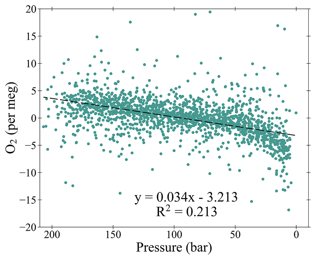
Figure 11 An aggregate of all the O₂ Working Tank (WT) mole fractions determined during all of the calibrations, plotted as the difference from the average mole fraction for each WT (measurement minus average) at WAO between May 2010 and December 2021, plotted versus the WT pressure. The linear trend line is denoted as a dashed black line. Note that five measurements are off scale, out of more than 1700 measurements shown.

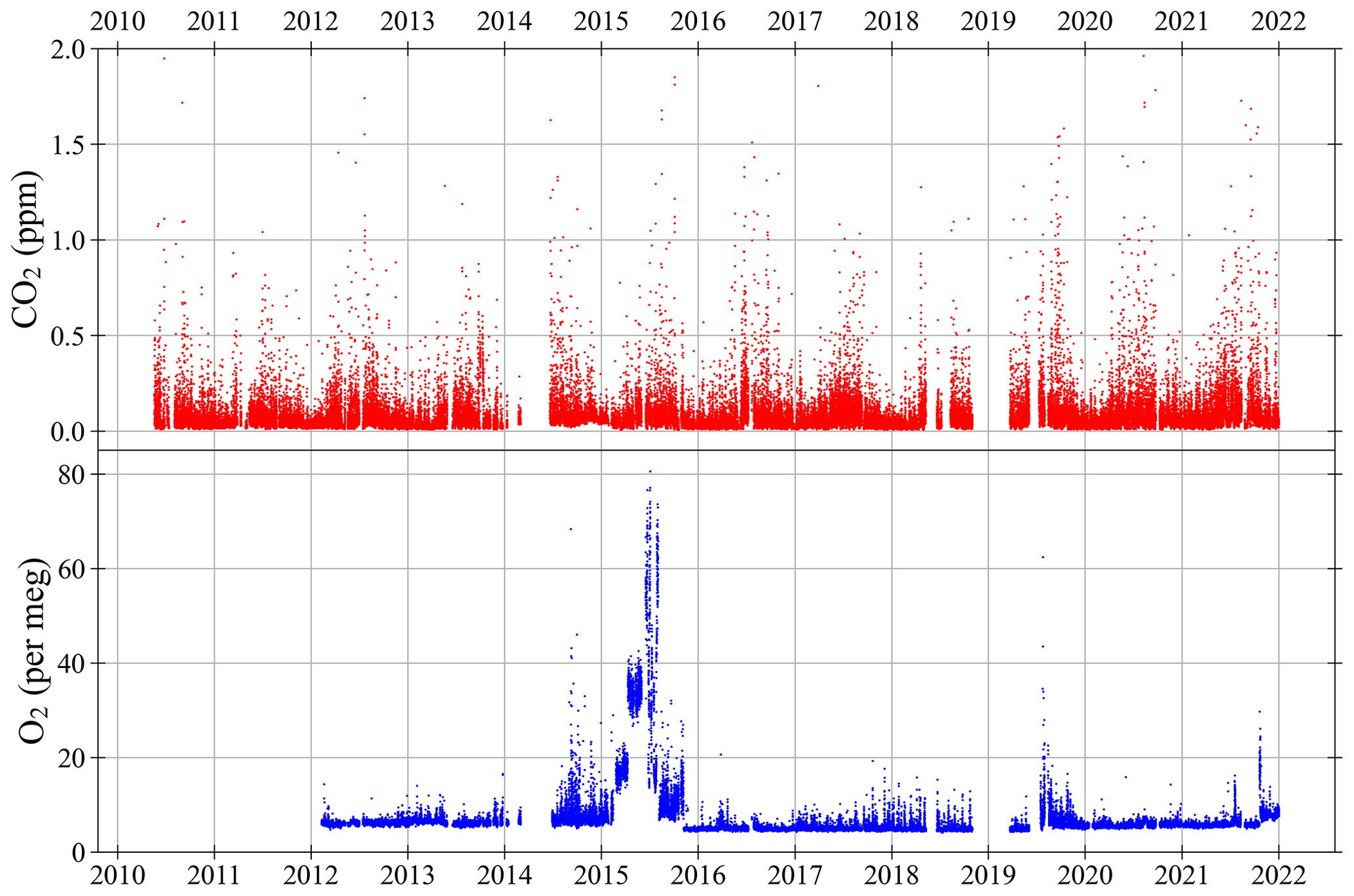
Figure 12 CO₂ (top panel) and O₂ (bottom panel) ±1σ standard deviation of air measurements at WAO between May 2010 and December 2021. The ±1σ standard deviations of the 2 min data were not routinely calculated for O₂ until February 2012. Hourly averages of the ±1σ standard deviations of the 2 min measurements. The O₂ y axis is not visually comparable on a mole per mole basis to the CO₂ y axis. Note that four measurements are off scale in the CO₂ panel, out of more than 70 000 measurements shown.

3.6 Standard deviation of the air measurements

Figure 12 shows the hourly averages of the ±1σ standard deviation of the 2 min measurements. For each 2 min measurement there is a ±1σ standard deviation, which is determined from the 1 min switching of WT and sample air, using 1 s data. These ±1σ standard deviations for each hour (30 data points if there are no gaps) are then used to calculate the mean. These ±1σ standard deviations include both the uncertainty in the measurement system and how much the actual CO₂ and O₂ mole fractions in the air vary over a 2 min period. Therefore, these ±1σ standard deviations cannot be compared to the ±1σ standard deviations of the Target Tanks or to the repeatability goals.

The ±1σ standard deviation of the CO₂ measurements is very stable over time (Fig. 12). On average the CO₂ ±1σ standard deviation is $\pm \mathrm{0.08}\pm \mathrm{0.10}$ ppm and is <0.2 ppm 93 % of the time. On average the O₂ ±1σ standard deviation is $\pm \mathrm{6.8}\pm \mathrm{5.4}$ per meg and is <10 per meg, 94 % of the time. In 2014 and 2015 the O₂ ±1σ standard deviation were much higher and more variable than usual, due to multiple different technical problems in 2014 and poorer performance of the Oxzilla analyser in 2015 (see Sect. 4.1). The 2014 and 2015 O₂ measurements are still accurate, as far as we can tell, but they are not as precise. In general, larger O₂ ±1σ standard deviations correspond to poorer performance of the Oxzilla analyser.

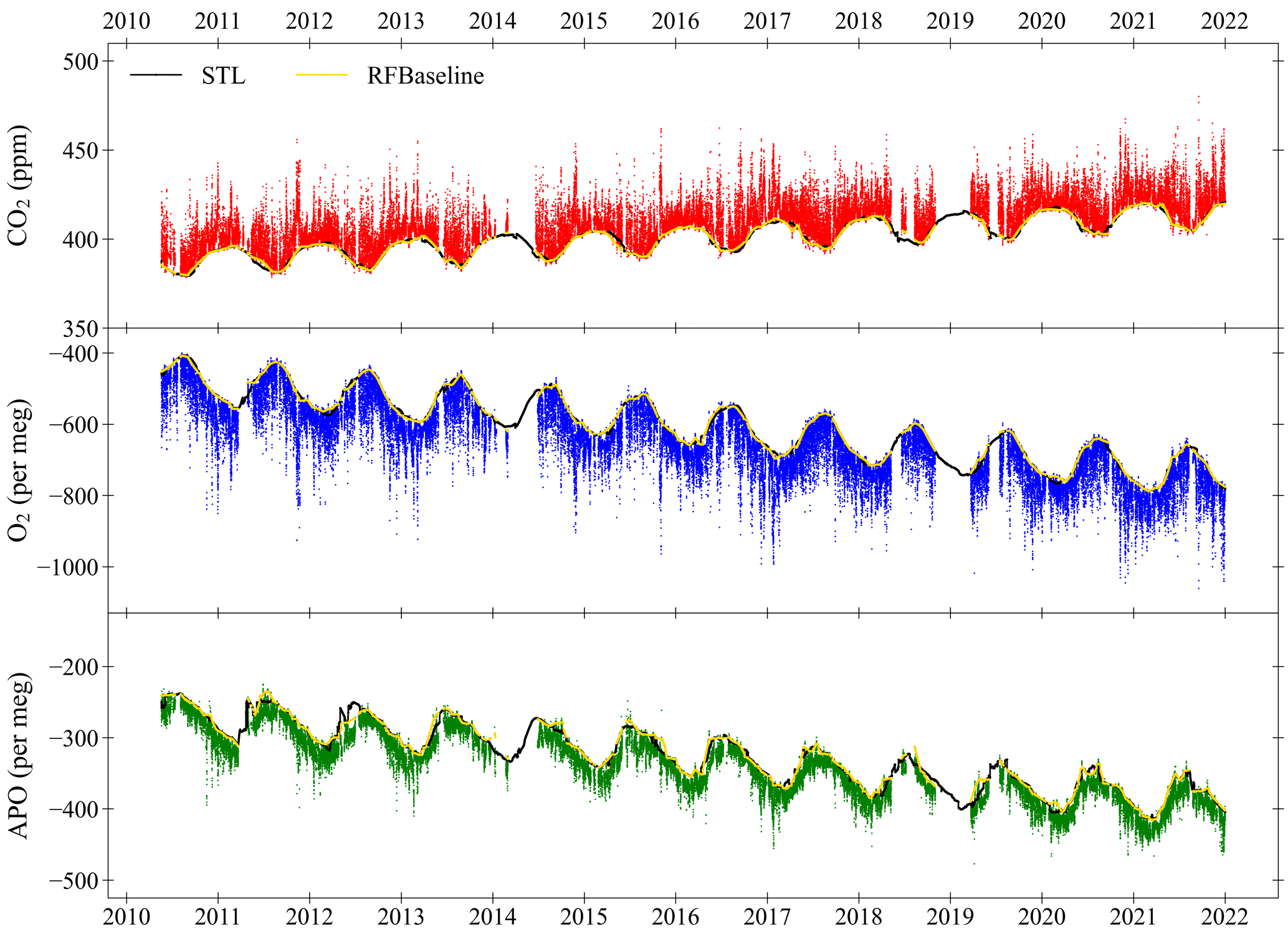
Figure 13 Hourly averaged CO₂ (top panel), O₂ (middle panel) and APO (bottom panel) at WAO between May 2010 and December 2021. The baselines (yellow lines) are fitted using the RFbaseline function of Ruckstuhl et al. (2012), and the curve fits (black lines) are calculated using the STL function in R (see Sect. 2.3). The O₂ and CO₂ y axes are scaled to be visually comparable on a mole per mole basis. The APO y axis is zoomed in two times, compared to the O₂ y axis on a mole per mole basis. The x axis tick marks are at the beginning of each year.

4 Key features of the WAO atmospheric CO₂, O₂ and APO data

4.1 Time series of CO₂, O₂ and APO

Figure 13 shows a 12-year time series from May 2010 to December 2021 of continuous in situ measurements of CO₂, O₂ and APO at WAO. Measurements continue to the present and are recorded every 2 min. There are gaps in the data caused by cylinder measurements (see Sect. 2.2), changing the WT, routine maintenance, and technical issues. Data collected when the system was experiencing known technical issues have been removed. In total there are 1 930 178 CO₂ measurements and 1 565 908 O₂ measurements (2 min frequency), from 19 May 2010 to 31 December 2021. The data have been averaged to hours to make the dataset more useful for typical applications. Hourly averages are only calculated when there are at least five 2 min measurements in an hour. There are 73 232 CO₂ hourly averages and 69 044 O₂ hourly averages, meaning that there are hourly measurements for 72 % (CO₂) and 68 % (O₂) of the time. Simultaneous measurements of both O₂ and CO₂ are needed to calculate APO.

The proportion of APO data missing in each year varies (Table 5). Measuring the WSSs, TTs, and ZTs takes approximately 14 % of the time in a year, so even if the measurement system ran perfectly, we would still not be able to measure air 100 % of the time. The most complete year was 2017, with only 15 % of the data missing. The year with the most missing data is 2014, where more than half (59 %) of the data are missing; the years 2015, 2018 and 2019 also have a large amount of missing data, 42 %, 46 % and 47 % respectively, due to multiple technical issues. All the other years have between 20 % and 33 % of the data missing (Table 5).

The technical issues in 2014 included: problems with the compressor that opened and closed the pneumatic valves (the on/off, three-way and four-way valves; Fig. 2), the pneumatic valves were replaced with solenoid valves in June 2014; in January and February there was no Ultramat signal because of a broken serial lead, and there was also no ZT; in May 2014 the WSS cylinders were changed; throughout the year there were electrical problems including with the USB hub, data acquisition boards and watchdog board; in June 2014 the red line inlet was blocked with sea salt; there was also a problem with the computer frequently crashing; the PC was replaced in November 2014. The year 2015 has a large amount of missing data, as this year also had technical issues, and a different Oxzilla analyser was used in this year which was not as precise.

The years 2018 and 2019 have a large amount of missing data, because between March 2018 to March 2019 the diaphragm in the KNF pump was torn causing the pump to leak. During this time only one of the inlet lines was being used so this leak affected all the data. Some of these data, from March 2018 to October 2018, were adjusted using the O₂ measurement record at Cold Bay Alaska, where we were confident of the offset caused by the pump and where we were additionally able to cross-check our correction against an independent dataset from a similar latitude (Shetlands Island, Scotland). However, the size of the leak increased over time, and data from November 2018 to March 2019 could not be adjusted with confidence and were flagged and removed from the quality-controlled dataset. More information on this leaking pump adjustment is provided in supplement.

Table 5 Annual mean of CO₂, O₂ and APO data at WAO from May 2010 to December 2021. The percentage of APO data missing each year based on the hourly averages is also shown (the APO calculation requires simultaneous CO₂ and O₂ measurements).

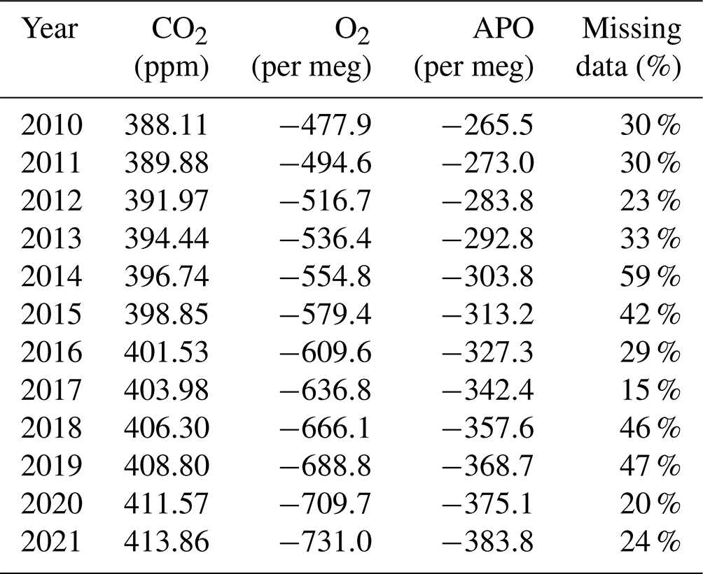
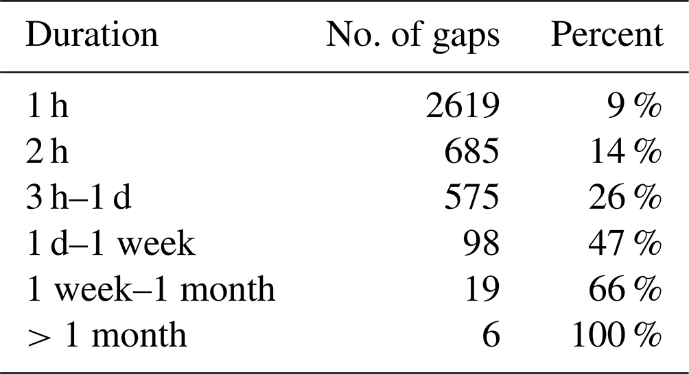
Most of the gaps in the data only last for short periods of time: 9 % of the missing data are due to gaps lasting 1 h and are usually caused by routine calibrations; 14 % of the missing data are due to gaps lasting 2 h; 26 % of the missing data are due to gaps lasting less than a day; 47 % of the missing data are due to gaps lasting less than a week; and 66 % of the missing data are due to gaps lasting less than a month (Table 6). There are six gaps in the data that last longer than a month. The largest gap in the data is 5 months long, and is it due to the data that had to be removed when the KNF pump was leaking between November 2018 and March 2019. The next longest gap is 4 months long and occurred in 2014 between 2 March and 28 June due to the combination of technical problems described above.

Table 6 Duration and number of gaps in the dataset, based on APO data.

From Fig. 13 we can see there are long-term trends in all three species. On average, atmospheric CO₂ at WAO increased by 2.40 ppm yr⁻¹ (2.38 to 2.42; 95 % confidence intervals), atmospheric O₂ decreased by 24.0 per meg yr⁻¹ (24.3 to 23.8), and APO decreased by 11.4 per meg yr⁻¹ (11.7 to 11.3). The long-term trends were calculated using the trend from the seasonal decomposition with STL (see Sect. 2.3) and the TheilSen function in the openair package in R (Carslaw and Ropkins, 2012; Carslaw, 2019). These long-term trends are predominantly due to the burning of fossil fuels and land-use changes, which release CO₂ and consume O₂. Atmospheric O₂ is decreasing more quickly than CO₂ is increasing because the globally averaged O₂:CO₂ exchange ratio for fossil fuel combustion is about 1.38 mol mol⁻¹ (Keeling and Manning, 2014), and the CO₂ increase is buffered by an increasing land carbon sink and ocean carbon sink, whereas the O₂ decrease is only buffered by an increasing land oxygen source and a small ocean oxygen source from O₂ outgassing (R. F. Keeling et al., 1996).

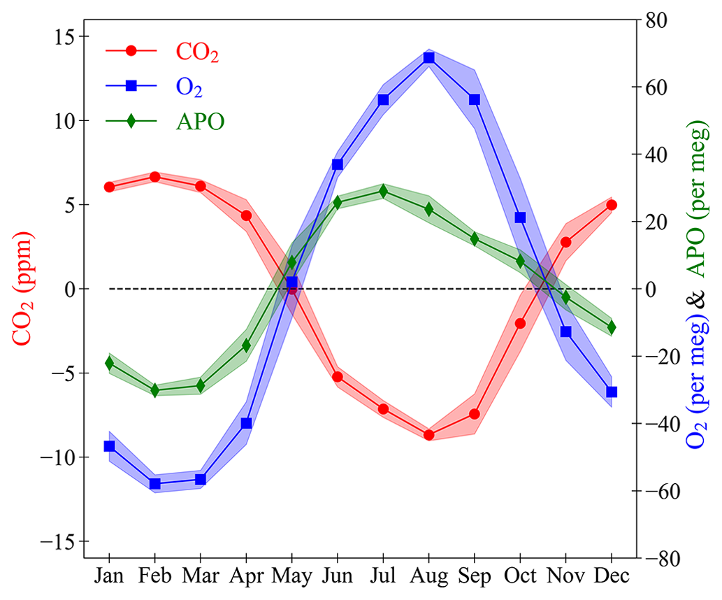
Figure 14 The seasonal cycles of CO₂ (red circles, left axis), O₂ (blue squares, right axis), and APO (green diamonds, right axis) at WAO. Individual points are the monthly means of the seasonal component of the STL decomposition (see Sect. 2.3). The shaded bands are the average of the ±1σ standard deviation of the monthly averages of the baseline data. The y axes are scaled to be visually comparable on a mole per mole basis.

4.2 Seasonal cycles

The seasonal component of the WAO time series is obtained using the STL decomposition (see Sect. 2.3). The CO₂ mole fraction is higher during the Northern Hemisphere winter and lower during the summer due mostly to the terrestrial biosphere (Fig. 14). Vegetation takes in CO₂ in the spring and summer in order to grow and releases CO₂ in the autumn and winter as it decomposes (Heimann et al., 1989). There is also an influence from increased temperature and sunlight during the summer leading to increased photosynthesis (Heimann et al., 1989). The exchange of CO₂ between the atmosphere and the oceans takes ∼1 year (Broecker and Peng, 1974), and O₂ fluxes from different ocean processes are reinforcing on seasonal timescales, whereas for CO₂ these counteract (Keeling and Manning, 2014). The combined effect of the CO₂ lag and counteracting CO₂ processes is that there is a minimal marine influence on the atmospheric CO₂ mole fraction seasonal cycle (Heimann et al., 1989; Randerson et al., 1997).

The O₂ mole fraction is lower during the winter and higher during the summer. O₂ is anti-correlated with CO₂ as they are involved in the same reactions, increased photosynthesis during the spring and summer releases O₂ and decomposition during the autumn and winter takes in O₂ (Keeling and Shertz, 1992). The air–sea gas exchange of O₂ is much quicker than for CO₂ and takes ∼1 month (Broecker and Peng, 1974). During the summer O₂ is outgassed from the oceans, and this enhances the O₂ seasonal cycle and makes it larger than the CO₂ seasonal cycle (Keeling and Shertz, 1992).

APO is lower during the winter and higher during the summer. The seasonal cycle of APO is correlated with the seasonal cycle of O₂ and anti-correlated with CO₂. APO is invariant to terrestrial biosphere processes. The seasonal cycle of APO is mainly driven by ocean ventilation changes, marine productivity cycling, and the changing solubility of O₂ in the oceans as temperature changes (Keeling et al., 1998). There is also a smaller effect on CO₂, O₂ and APO from the seasonal cycle of fossil fuel emissions as more fossil fuel combustion takes place during the winter for heating and lighting (Steinbach et al., 2011). There is also a seasonal cycle in the height of the atmospheric boundary layer, that influences all three species (Stephens et al., 2000). The APO seasonal cycle is about half the size of the O₂ cycle ($\mathrm{68}/\mathrm{134}=\mathrm{0.5}$) indicating that about half of the O₂ seasonal cycle at WAO is due to terrestrial biosphere processes and about half is due to ocean processes and fossil fuel combustion.

The CO₂ maximum, O₂ minimum and APO minimum occur between January and March each year. The CO₂ minimum and O₂ maximum occur in August or September each year. The APO maximum is more variable and tends to occur earlier in the year between June and August. The peak-to-peak amplitude of the seasonal cycle for CO₂ is 16 ppm (15 to 17 ppm), for O₂ it is 134 per meg (128 per meg to 139 per meg), and for APO it is 68 per meg (62 per meg to 73 per meg). A zero-crossing day is the date at which the detrended curve crosses zero on the y axis (C. D. Keeling et al., 1996). Spring zero crossings occur in April or May each year, and the autumn zero crossings in October or November each year.

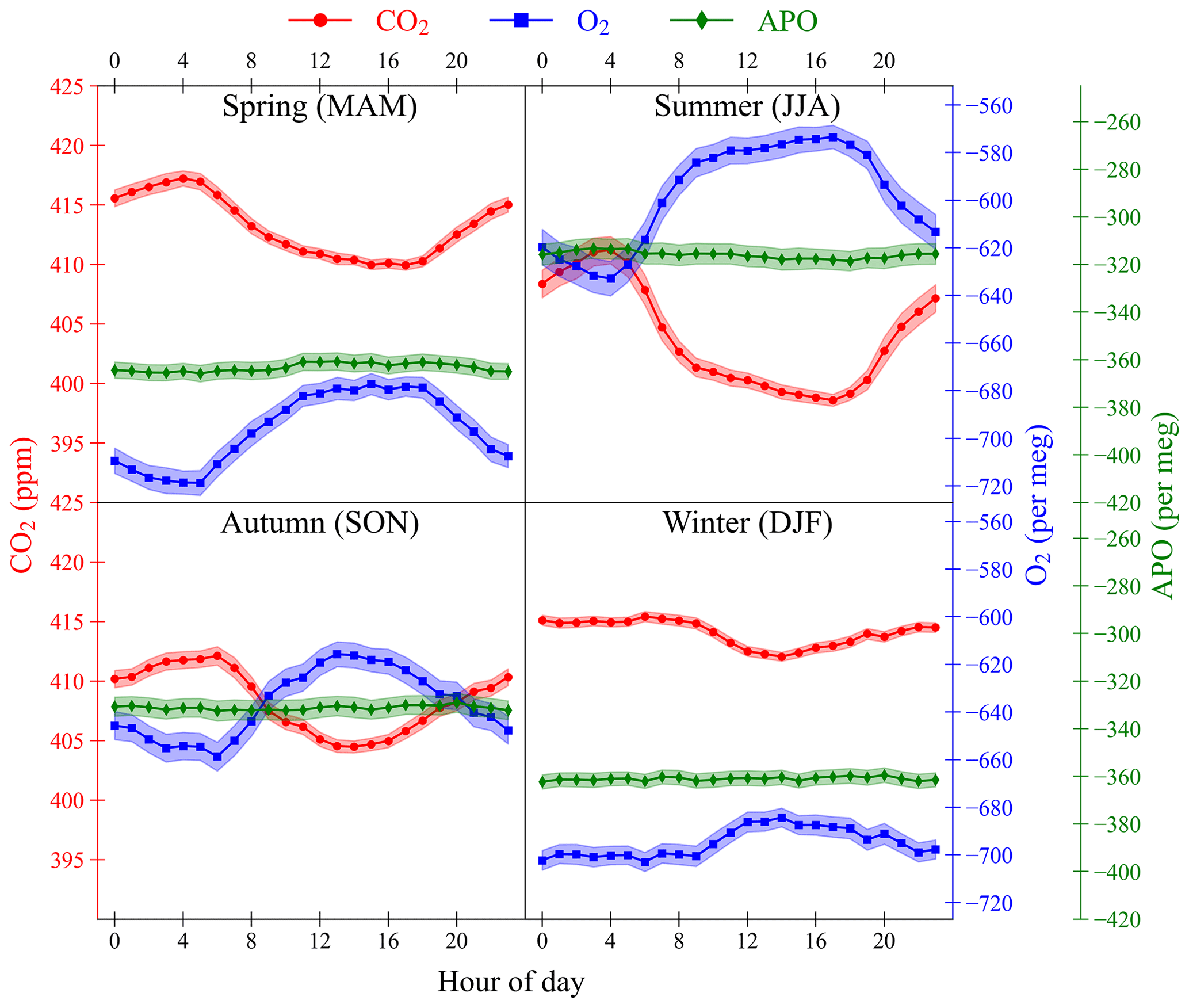
Figure 15 The diurnal cycles of CO₂ (red circles, left axis), O₂ (blue squares, right axis), and APO (green diamonds, right axis) at WAO for each season: spring (MAM), summer (JJA), autumn (SON), and winter (DJF). Individual points are calculated using the 2 min data from May 2010 to December 2021, with the timeVariation function in the OpenAir package in R (Carslaw and Ropkins, 2012). The shaded bands are the average of the ±1σ standard deviation of the hourly averages of the data. The y axes are scaled to be visually comparable on a mole per mole basis.

4.3 Seasonal variability of diurnal cycles

In general, CO₂ mole fractions are lower during the day and higher at night (Fig. 15). O₂ mole fractions are anti-correlated with CO₂ and are higher during the day and lower at night. APO variations do not exhibit a diurnal cycle at WAO. The diurnal cycles in CO₂ and O₂, like the seasonal cycles, are influenced by changes in the terrestrial biosphere processes of photosynthesis and respiration driven by changes in sunlight and temperature and are influenced by changes in the atmospheric boundary layer height (Stephens et al., 2000; Kozlova et al., 2008). The atmospheric boundary layer is higher during the day and lower during the night, which causes a dilution effect, as molecules during the day are spread out over a larger volume (Denning et al., 1996; Larson and Volkmer, 2008). This amplifies the diurnal cycles in O₂ and CO₂ mole fractions and is referred to as the diurnal rectifier effect. Temperature variations in the oceans that affect gas solubility are not observable on diurnal timescales due to the higher heat capacity of water that can buffer temperature changes.

APO at WAO does not have a diurnal cycle because it is not influenced by the terrestrial biosphere; atmospheric boundary layer effects tend to cancel for APO on diurnal scales, since APO is the sum of two strongly anti-correlated species; and WAO is too remote for APO at the site to be influenced by the diurnal cycle in fossil fuel sources.

There are differences in the diurnal cycles in different seasons. The average amplitude of the diurnal cycles of CO₂ and O₂ are largest in the summer (CO₂: 12.6 ppm, O₂: 60 per meg) and smallest in the winter (CO₂: 3.4 ppm, O₂: 19 per meg). This is due to the combined effect of the diurnal cycle and the seasonal cycle. In the summer, there are higher temperatures, more sunlight and longer days leading to more terrestrial biosphere productivity and larger changes in atmospheric boundary layer height as the differences in temperature between night and day are larger (Bakwin et al., 1995).

In the spring terrestrial productivity is starting to increase, and in the autumn it is starting to decrease as plants die, lose their leaves and become less active. In the winter there are lower temperatures, less sunlight, and shorter days, leading to less activity in the terrestrial biosphere. Also, changes in atmospheric boundary layer height are smaller in the winter as the differences in temperature between the night and day are smaller, so the diurnal rectifier effect is less pronounced (Bakwin et al., 1995). So, the amplitudes of the CO₂ and O₂ diurnal cycles are smallest in the winter.

There are more hours of sunlight during the summer than during the winter, so the summer has a broader peak in O₂ and trough in CO₂ during the day and a shorter peak and trough in the winter. This also effects the timing of the maxima and minima. The CO₂ maximum and O₂ minimum occurs earlier in the summer, at about 04:00, than in the winter, at about 06:00. The CO₂ minimum and O₂ maximum occurs later during the summer at about 17:00 and earlier in winter at about 14:00. Winter CO₂ and O₂ are mostly flat during the night from about 21:00 to 09:00 as the amount of respiration stays mostly the same during the day and the night.

5 Data availability

The accompanying database comprises one csv file. The file contains information on the CO₂, O₂, and APO data (values and associated uncertainties) from Weybourne Atmospheric Observatory.

The file is published by the ICOS Carbon Portal, and is available at https://doi.org/10.18160/Z0GF-MCWH (Adcock et al., 2023).

Other data presented in this paper are available upon request.

6 Conclusions

We have presented a 12-year time series of continuous measurements of CO₂, O₂ and APO at Weybourne Atmospheric Observatory (WAO) in the United Kingdom. The results from the GOLLUM, Cucumbers, and WMO Round Robin intercomparison programmes show that WAO is sometimes but not always within the O₂ and CO₂ WMO compatibility goals established by the high-precision greenhouse gas measurement community. Measurements of Target Tanks indicate that the 2 min O₂ repeatability is $\pm \mathrm{3.0}\pm \mathrm{4.6}$ per meg, averaged over the 12 years, which is within the extended repeatability goal of ±5 per meg. Target Tanks CO₂ repeatability is $\pm \mathrm{0.005}\pm \mathrm{0.023}$ ppm, which is an order of magnitude below the repeatability goal (±0.05 ppm). Measurements of Zero Tanks indicate that the O₂ repeatability is $\pm \mathrm{3.1}\pm \mathrm{5.3}$ per meg, and the CO₂ repeatability is $\pm \mathrm{0.005}\pm \mathrm{0.019}$ ppm, which is similar to the repeatability indicated by the Target Tank measurements. We also show that the calibration coefficients vary over time and the R² of the O₂ calibration fit is >0.995, 92 % of the time. The Working Tanks show that O₂ mole fractions decrease in a cylinder as the pressure decreases. The ±1σ standard deviations of the air measurements for CO₂ are on average $\pm \mathrm{0.08}\pm \mathrm{0.10}$ ppm, based on the hourly averages, and are very stable for the whole time series, while the ±1σ standard deviations for the O₂ air measurements are more variable. Measurements are made every 2 min and between May 2010 and December 2021 there are 1 930 178 CO₂ measurements and 1 565 908 O₂ measurements. There are gaps in the dataset caused by regular calibrations, routine maintenance, and technical issues, and there are six gaps over the 12-year period that last longer than a month. Multiple technical issues in 2014 and 2015 decreased the precision of the data. There are no periods when the Target Tanks, Zero Tanks, and calibration coefficients are all drifting at the same time, indicating that the calibration scale at WAO is likely stable. The time series shows average long-term trends of 2.40 ppm yr⁻¹ (2.38 to 2.42) for CO₂, −24.0 per meg yr⁻¹ (−24.3 to −23.8) for O₂, and −11.4 per meg yr⁻¹ (−11.7 to −11.3) for APO. The average seasonal cycle peak-to-peak amplitude for CO₂ is 16 ppm (15 to 17), for O₂ it is 134 per meg (128 to 139), and for APO it is 68 per meg (62 to 73). The average amplitude of the diurnal cycle in summer is 12.6 ppm for CO₂ and 60 per meg for O₂, and the amplitude of the diurnal cycle in winter is 3.4 ppm for CO₂ and 19 per meg for O₂.