The DTU21 global mean sea surface and first evaluation

A new mean sea surface (MSS) from the Technical University of Denmark (DTU) called DTU21MSS for referencing sea-level anomalies from satellite altimetry is introduced in this paper, and a suite of evaluations are performed. One of the reasons for updating the existing mean sea surface is the fact that during the last 6 years, nearly 3 times as many data have been made available by space agencies, resulting in more than 15 years of altimetry from long-repeat orbits (LROs) or geodetic missions. This includes the two interleaved long-repeat cycles of Jason-2 with a systematic cross-track distance as low as 4 km.

A new processing chain with updated filtering and editing has been implemented for the DTU21MSS. This way, the DTU21MSS has been computed from 2 Hz altimetry in contrast to the former DTU15MSS and DTU18MSS which were computed from 1 Hz altimetry. The new DTU21MSS is computed over the same 20-year averaging time from 1 January 1993 to 31 December 2012 with a well-specified central time of 1 January 2003 and is available from https://doi.org/10.11583/DTU.19383221.v1 (Andersen, 2022).

Cryosat-2 employs synthetic aperture radar (SAR) and SAR interferometric (SARin) modes in a large part of the Arctic Ocean due to the presence of sea ice. For SAR- and SARin-mode data we applied the SAMOSA+ physical retracking to make it compatible with the physical retracker used for conventional low-resolution-mode data in other parts of the ocean.

1 Introduction

Satellite altimetry provides highly accurate measurements of the ocean topography along the ground tracks of the satellite (Fu and Cazenave, 2001; Stammer and Cazenave, 2017). For oceanography, the anomalous sea level about a mean reference surface is of primary interest. During the last 2 decades, a mean sea surface (MSS) as a reference surface has been developed with increasing accuracy (Pujol et al., 2017; Yuan et al., 2023).

Mean sea surface models are increasingly used as vertical offshore reference surfaces for offshore operations (e.g., dredging, wind farms, bathymetry surveys).

To develop a MSS it would be optimal if observations were available on all temporal and spatial scales. The challenge is to derive an MSS given limited sampling in both time and space using satellite observations. Another challenge is to merge repeated observations along coarse ground tracks with high spatial data from geodetic missions (GMs).

Thanks to new altimeter instruments and processing technology, the accuracy of observed sea surface height (SSH) has increased dramatically over the last decade. Sea-level anomalies (SLAs) are referenced to a global MSS. It is consequently important that the MSS is as accurate as possible when investigating smaller mesoscale features (e.g., Dufau et al., 2016).

The paper is structured in the following way. Section 2 presents the details of the derivation of the new DTU21MSS from the Technical University of Denmark (DTU) with a focus on the improvement in data, retracking, processing and filtering. The chapter is concluded with a subsection on the potential use of synthetic aperture radar (SAR) altimetry from Sentinel 3A and 3B for the DTU21MSS. Section 3 highlights various comparisons ranging from global comparison to regional evaluations in the Arctic Ocean and for coastal regions illustrating the improvement in the DTU21MSS model.

2 Computation of the DTU21MSS

The DTU21MSS is based on satellite altimetry data from frequently repeating exact-repeat missions (ERMs) and infrequent missions with a long or drifting repeat – called a geodetic mission (GM). The MSS is determined from a sophisticated combination of the coarse ERM with the high-density GM data as described in Andersen and Knudsen (1998, 2009; Andersen et al., 2010). ERM data are used to derive the coarse MSS. Subsequently, the GM data are introduced to derive the fine-scale features in the MSS.

The long-wavelength MSS was derived using the highly accurate nearly uninterrupted mean profiles derived using TOPEX (TP), Jason-1 (J1) and Jason-2 (J2). These data were taken from the 1 Hz data from the Radar Altimetry Database System (RADS; Scharroo et al., 2013). To extend the MSS into the polar regions outside the 66^∘ parallel and to enhance the spectral resolution the other mean profiles shown in Table 1 from other exact-repeat satellites were fitted to the TOPEX, J1 and J2 profiles. The differences were found by computing crossover differences between the ERM datasets. The crossover residuals were expanded into spherical harmonic degrees and order 2 to 4, and this surface was used to correct the ERM datasets. This methodology was similarly applied to derive the DTU15MSS and DTU18MSS. Hence as a prior long-wavelength model, we used a filtered version of the DTU18MSS for wavelengths greater than 100 km. For reference, the filtered versions of the DTU18MSS and DTU15MSS are virtually identical inside the 66^∘ parallel.

Before the MSS is computed, the averaging period, and consequently the center time, for the MSS was selected. We used an averaging period from 1 January 1993 to 31 December 2012. Hence the center time for the DTU21MSS and previous DTU models will be 1 January 2003.

There has been a significant focus on the accuracy of MSS models (Pujol et al., 2017) in the preparation for the Surface Water and Ocean Topography (SWOT) mission, launched recently. We consequently decided to keep the same 20-year averaging period for the DTU21MSS to be able to validate the MSS directly with other MSS models. Changing the averaging period by as little as 3 years will change the mean by 1 cm as well as the spatial pattern due to ongoing sea-level change (Veng and Andersen, 2021).

Table 1 shows all altimetry used for the computation of the DTU21MSS and its predecessors: the DTU15MSS and DTU18MSS. Whereas the DTU15MSS was based on roughly 5 years of GM observations, the DTU21MSS is based on nearly 3 times as many data or more than 15 years of GM due to the recent focus on prioritizing long-repeat orbits (LROs).

Satellite observations from the four newer GMs (Cryosat-2, Jason-1, Jason-2 and SARAL) have a range precision around 1.5 times higher than the old ERS-1 and Geosat GM (Garcia et al., 2014). Consequently, it was decided to retire the older ERS1 and Geosat GM data for the DTU21MSS.

Table 1 Satellite altimetry used for the DTU15, DTU18 and DTU21MSS models.

The following sections describe the theoretical and practical advances leading up to the release of the DTU21MSS. The next section describes the short-wavelength improvement and the subsequent section the improvement to the long-wavelength part in the polar regions.

2.1 The short-wavelength MSS from geodetic mission altimetry

The short-wavelength part of the MSS is derived from geodetic mission (GM) data. The Sensor Geophysical Data Record (SGDR) products for Jason-1 GM, Jason-2 GM and SARAL/AltiKa GM are obtained from the Archiving, Validation and Interpretation of Satellite Oceanographic (AVISO) data service. The L1b-level products for the CryoSat-2 low-resolution mode (LRM) are acquired through the data distribution service of the European Space Agency (ESA). All these products include along-track 20 Hz waveforms for all missions except for 40 Hz waveforms for SARAL/AltiKa.

All environmental and geophysical corrections of the altimeter range measurements have been applied to calculating SSH (Andersen and Scharroo, 2011). These corrections include dry and wet tropospheric path delay, ionospheric correction, ocean tide, solid earth tide, pole tide, high-frequency wind effect, and inverted barometer correction. The most recent FES2014 ocean tide model has been used for all missions (Lyard et al., 2021). All corrections are provided to 1 Hz. Hence, these were interpolated into 20 or 40 Hz using piecewise cubic spline interpolation.

All satellites except for CryoSat-2 operate in the traditional LRM, where the along-track resolution is limited to 2–3 km. Cryosat-2 also operates in LRM over most of the oceans.

In regions where sea ice is prevailing, Cryosat-2 operates in synthetic aperture radar (SAR) mode. In this mode, the returning echoes are processed coherently, resulting in a footprint of 290 m. Over steeply varying terrain and in some coastal regions, the SAR interferometric mode (SARin) is used where the instrument receivers on two antennas are used. A mode mask controls the availability of three Cryosat-2 data types (web1, 2023). The advantage of SAR processing is an improvement of nearly 2 times the range precision (Raney, 2011). Due to the burst structures of Cryosat-2, the improvement found is only around 1.5 times the range precision of LRM data (Raney, 2011; Garcia et al., 2014).

Waveform retracking is an effective strategy to improve the range precision of altimeter echoes (Gommenginger et al., 2011). There are two strategies. Empirical retrackers have the advantage of providing a valid and robust estimation of arrival time used to determine the SSH over almost all types of surfaces (e.g., sea ice leads, coastal). The disadvantage is that empirical retrackers only provide SSH and not rise time, used to determine significant wave height and wind speed. Hence it is not possible to determine the sea state bias correction to the SSH observations (Fu and Cazenave, 2001).

Physical retrackers generally apply the Brown model for LRM data (Brown, 1977) or the SAMOSA model for SAR and SAR-in observations (Ray et al., 2015). These retrackers estimate three or more parameters and enable corrections and sea state conditions, through the determination of significant wave height and wind speed. Hence these enable the determination of, and subsequent correction for, sea state bias correction.

2.1.1 Two-pass retracking for range precision

Over the ocean, the waveforms from all four GM satellite missions are well modeled and retracked using the Brown-type model. In the first step, the waveforms are fitted by the three-parameter Brown model (arrival time, rise time, and amplitude).

Maus et al. (1998) and Sandwell and Smith (2005) demonstrated the presence of a strong coherence between the estimation errors in the arrival time and rise time parameters, resulting in a relatively noisy estimate of arrival time and hence sea surface height. Consequently, Sandwell and Smith (2005) suggested the use of a second step where the rise time parameter is smoothed. In the derivation of the DTU21MSS, we applied the same two-step retracking and fixed the along-track smoothing at 40 km before retracking the waveforms again using a two-parameter waveform model (fitting only arrival time and amplitude).

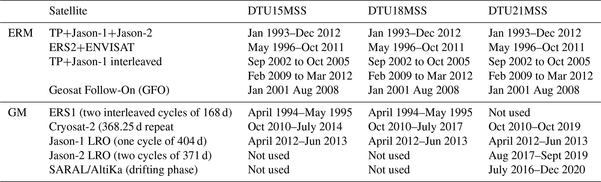
For all four recent GM missions (Jason-1, Jason-2, SARAL/AltiKa and CryoSat-2/LRM), this approach has been proved effective (Garcia et al., 2014; Zhang and Sandwell, 2017; Andersen et al., 2021). Figure 1 illustrates the gain in range precision using the two-pass retracking. The improvement for all four LRM datasets is dependent on the SWH but is on average of the order of 1.5, similar to other studies (Sandwell et al., 2014; Zhang et al., 2020).

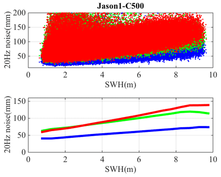
Figure 1 The standard deviation of retracked height with respect to the DTU15MSS for cycle 500 (corresponds to the first 11 d of the Jason-1 GM). The upper figure illustrates the statistics for individual points. The lower figure illustrates the median averaged over 0.5 m SWH intervals. Red: height from sensor geophysical data record. Green: height from the first step of two-pass retracking. Blue: height from the second step of the two-pass retracking. Modified from Andersen et al. (2021).

Whereas two-pass retracking is very efficient for improving the range precision for the LRM data, we did not apply the two-pass retracking for the CryoSat-2 SAR- and SARin-mode data as there is no gain in range precision from the second step of the retracking for SAR and SARin data. This was first documented by Garcia et al. (2014).

2.1.2 2 Hz sea surface height data

The 20 or 40 Hz double-retracked SSH data are edited for outliers, and subsequently, an along-track low-pass filter is applied before generating the 2 Hz SSH data used for the subsequent MSS determination.

The along-track low-pass filter uses the Parks–McClellan algorithm which has a cut beginning at 10 km wavelength and zero gain at 5 km; thus the filter has 0.5 gain at 6.7 km, which is approximately the along-track resolution of 1 Hz data (Sandwell and Smith, 2009). The filter had to be designed for each satellite mission to match the 0.5 gain at 6.7 km due to the different along-track sampling rates. After this filter is applied the data were downsampled to a 2 Hz sampling rate, which corresponds to an along-track spacing of around 3.3 km.

For the previous DTU15MSS, we used 1 Hz SSH data from the Radar Altimetry Database System (RADS; Scharroo et al., 2013). In RADS, the 1 Hz data are computed as the average of all 20 Hz data, which is equivalent to using a boxcar filter. The disadvantage of this filer is that spectral leakage in the 10–40 km wavelength, which will remain as high-frequency noise in the filtered dataset, contributes to the spectral hump of conventional LRM data (Dibarboure et al., 2014; Garcia et al., 2014). The advantage of using the Parks–McClellan algorithm over the boxcar filter is that this filter has better spectral gain. The filter characteristics are illustrated in Fig. 2 for both filters.

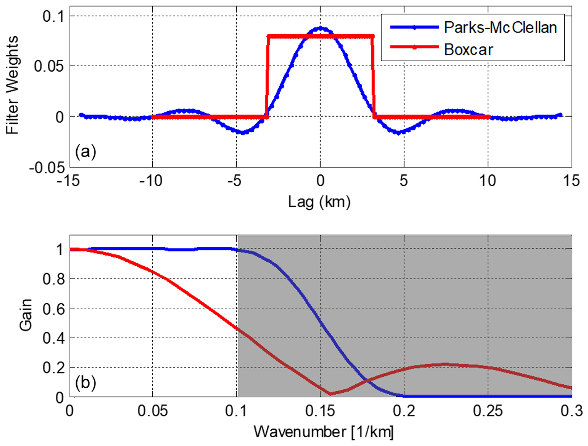
Figure 2 Illustration of Parks–McClellan filter weights (blue) and the boxcar filter (red) to derive the 1 or 2 Hz SSH data spatial filter (a). Panel (b) illustrates the frequency response of the two filters. Sidelobes and spectral leakage in the 10–40 km wavelength can be seen for the boxcar filter, which will remain as high-frequency noise in the filtered dataset.

2.2 Long-wavelength polar-region MSS improvements

For the polar regions, we used the filtered version of the DTU15MSS as a prior long-wavelength reference. The reason is that the DTU18MSS was based on empirical retracked height in the polar regions. Frequently, physical and empirical retrackers differ in their height estimation in polar regions (Rose et al., 2019). The DTU15MSS was based on sparse physical retracked data from RADS. However, it was found to be a more consistent prior choice for the DTU21MSS where physical retracking is used.

Cryosat-2 provides observations all the way to 88^∘ N. A closer inspection of the Cryosat-2-mode mask (web1, 2022) shows that polar regions (outside the 66^∘ parallels) are largely measured in the SAR and SARin modes due to the presence of sea ice. This is with the exception of the Barents Sea, north of Norway.

For SAR- and SARin-mode data, we applied the SAMOSA+ physical retracking (Dinardo et al., 2018). SAMOSA+ adapts the SAMOSA retracking model (Ray et al., 2015) to operate over specular scattering surfaces as ice-covered polar oceans by involving the mean square slope as an additional parameter in the retracking scheme and by implementing a more sophisticated choice of the fitting initialization, resulting in greater robustness to strong off-nadir returns from land. The SAMOSA+ retracker even discriminates between return waveforms from diffusive and specular scattering surfaces, ensuring the continuity in the sea-level retrieval going from the open ocean and into the leads in the sea ice.

Figure 3 The DTU21MSS and DTU15MSS for the Southern Ocean (a) and the Arctic Ocean (b). The color scale ranges up to ±5 cm for the Southern Ocean and ±10 cm for the Arctic Ocean.

With the assistance of the European Space Agency (ESA) Grid Processing On Demand (GPOD), we have processed a total of 9 years of Cryosat-2 (October 2010 to October 2019) for both the Arctic and the Southern Ocean using this SAMOSA+ retracker. Observations over the sea ice–open-ocean interface were removed in the processing, and only observations over leads (ocean surface between the ice floes) were selected similar to Rose et al. (2019).

Upon computing the mean profiles of Cryosat-2 observations, the center time for the Cryosat-2 data was April 2015. It was found that it was necessary to correct for sea-level rise to consolidate these data from the January 2003 center period of the DTU21MSS following the methodology by Rio and Andersen (2009). This was performed in the 65–66^∘ border zone as the reprocessing of Cryosat-2 with SAMOSA+ is limited to outside the 65^∘ parallels. This resulted in a correction of a few centimeters.

The difference between the DTU21MSS and DTU15MSS is shown in Fig. 3 for both the Southern Ocean and Arctic Ocean. For nearly all ice-covered regions, the DTU15MSS is higher than the DTU21MSS. We expect this to be due to the fact that the DTU15MSS was derived from 1 Hz RADS data, which was very sparse in both time and space. The few data in RADS are a consequence of tight editing and the fact that RADS converts the SAR data to pseudo LRM (Scharroo et al., 2013) and performed physical retracking on these data using a modified Brown model. In RADS, we nearly only found data during the ice-free summer month when the annual signal causes the sea level to be higher, so it is expected that the DTU15MSS could be biased high due to this.

2.3 Mean sea surface computation

The details of the computation technique of the DTU21MSS follow the development of former DTU MSS models (Andersen and Knudsen, 2009), where the ERM tracks are first used to compute the long-wavelength part of the MSS as shown in Sect. 2.2. Hereafter the GM data are introduced to compute the fine-scale structures of the MSS. The fine-scale computation is done in small tiles of $\mathrm{1}{}^{\circ }\times \mathrm{3}{}^{\circ }$, with a 0.5^∘ boundary to parallelize the computation process. As all wavelengths longer than the size of the tiles are removed in this process (roughly 200 km), we found that there was no need to adjust the period of the GM data to the MSS averaging period (1993–2012).

The final step to close the polar gap is to fill in MSS proxy data north of 88^∘ N where no altimetry is available. This was done by feathering the EGM08 geoid (Pavlis et al., 2012) across the pole in the following way: the preliminary MSS was calculated up to 88^∘ N using the satellite altimetry data alone. Subsequently, the difference between the MSS and the EGM08 geoid was computed longitude-wise in the 87–88^∘ N region, and a mean offset was estimated and removed. The residual grid was transformed into a regular grid in polar stereographic projection enabling interpolation across the North Pole using a second-order Gauss–Markov covariance function with a correlation length of 400 km. This makes the DTU MSS models truly global.

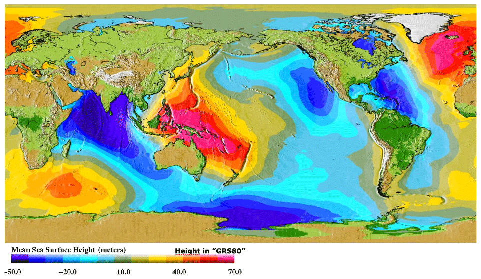
Figure 4 The DTU21 mean sea surface from the Technical University of Denmark (DTU) in meters.

The DTU21MSS as its predecessors are all given on a 1 min global resolution grid. A closer examination of the MSS in Fig. 4 illustrates that the height of the ocean's mean sea surface relative to the mathematical best-fitting rotational symmetric reference system (GRS80) has magnitudes of up to 100 m.

2.4 Sentinel 3A and 3B SAR altimetry

The European Space Agency (ESA) launched Sentinel 3A on the 16 February 2016 and Sentinel 3B on 25 April 2018. These satellites operate as SAR altimeters everywhere with the benefit of increased range precision compared with conventional LRM altimetry. Both the increased along-track resolution and more importantly the improved cross-track resolution of 35 km for the combined Sentinel 3A and 3B dataset would make these important contributors to the DTU21MSS. However, two problems prevented the use of these data for the time being.

The first relates to the fact that mean profiles could only be computed over 5 and 3 years from Sentinel 3A and B, respectively. As the Sentinel 3 satellites operate in a 27 d repeat orbit, this resulted in as few as 66 and 40 cycles, making these mean profiles considerably noisier compared with other mean profiles. Secondly, the center times of Sentinel 3A and 3B are 2019 and 2020, which means that the mean profiles are more than 15 years away from the center time of the TOPEX, J1 and J2 mean profiles. We illustrate the problem in Fig. 5 from a section of the Gulf Stream. The mean of S3A is 8 cm, but the standard deviation of the spatial variation with respect to the DTU15MSS is as high as 13 cm (Fig. 5 left panel). We show the mean profile from Sentinel 3A along track 719 (located between the blue arrows in the left panel) across the Gulf Stream going from south to north (right panel of Fig. 5). Between 26 and 32^∘ N, the difference corresponds closely to the expected sea-level rise of a little more than 8 cm. However, as the track crosses the Gulf Stream, the signal increases to nearly 60 cm.

The mean dynamic topography associated with the Gulf Stream causes the mean sea level to drop by around a meter as one moves from the center of the northwestern Atlantic toward the coast. Due to the north–south meandering of the Gulf Stream, it creates the observed sea-level residual seen when the averaging period changes (Zlotniki, 1991).

As Sentinel 3A and 3B are both outside the 1993–2012 averaging period and as the meandering of the Gulf Stream is profound over the last 15 years, it was not possible to ingest the S3A and B mean profiles without degrading the DTU21MSS in this region.

There is no doubt about the importance of Sentinel 3A and 3B for future MSS models, but to ingest Sentinel 3A and 3B in future MSS models, we found that we will need to extend the averaging period to 30 years (1993–2022). We consequently decided only to use the Sentinel 3A and 3B for the evaluation of the various MSS models.

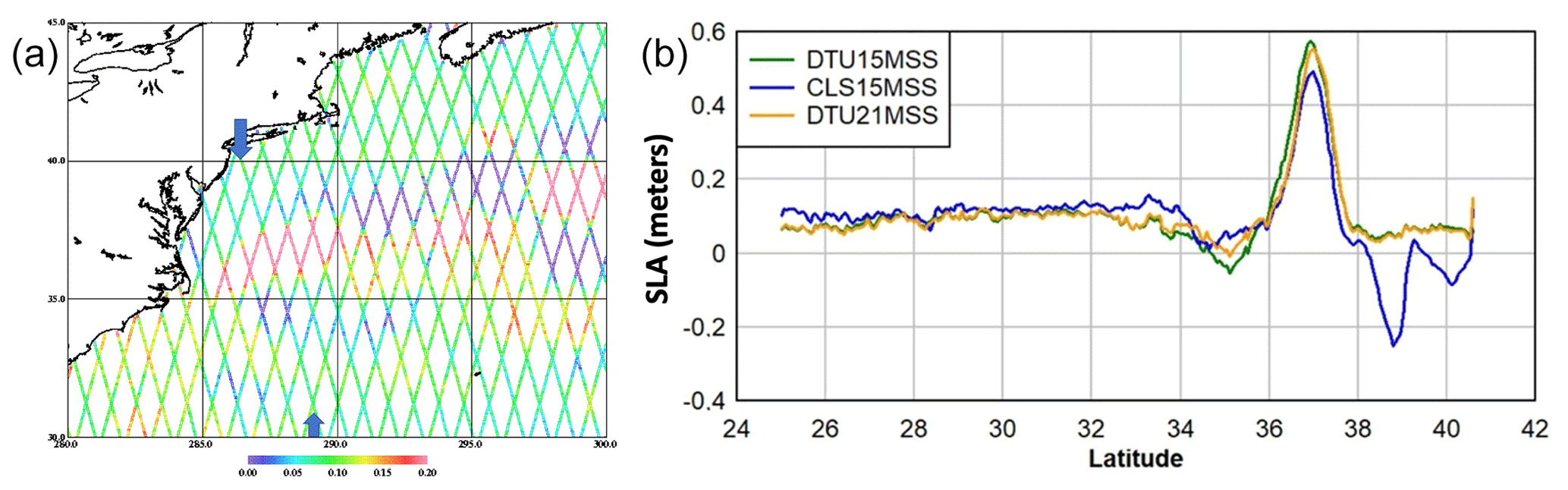
Figure 5 Sentinel 3A 5-year mean sea-level anomaly along track 791 in the Gulf Stream area relative to the DTU15MSS (a). Sentinel 3A track 791 is located between the blue arrows in (a). The S3A mean anomalies relative to the DTU15MSS, CLS15MSS and DTU21MSS (b).

3 Evaluation

In this section, we perform three different evaluations of the MSS. These evaluations supplement the global evaluation of previous MSS models performed by Pujol et al. (2017) and serve the purpose of indicating the improvements going from the DTU15MSS to the DTU21MSS globally, in the Arctic Ocean and in coastal regions. The CLS15MSS is an improvement of the CLS11MSS (Schaeffer et al., 2012) and is given on a similar $\mathrm{1}/\mathrm{60}{}^{\circ }$ resolution with a similar averaging period to the DTU MSS models (Pujol et al., 2017). Hence the various MSS models can be directly compared.

3.1 Global evaluation with mean profiles

In the global evaluation, we used data from the 1 Hz RADS data archive. The global comparison in Table 2 illustrates the mean difference and the spatial variation when the mean profiles are spline-interpolated onto the various MSS models. The zero offset and small standard deviation for the TP, J1 and J2 mean profile are because all MSS models are fitted to this profile in its derivation. The small offset for the other mean profiles corresponds to the fact that the averaging of these profiles is not centered directly on January 2003. The increased spatial standard deviation for other mean tracks is a consequence of fewer repeat cycles available for these missions, fewer than 200 cycles versus 1000 repeat cycles for the TP, J1 and J2 mean profiles.

Table 2 Comparison with mean profiles given as mean difference and standard deviation (in parentheses) of spatial variations. All values are in centimeters.

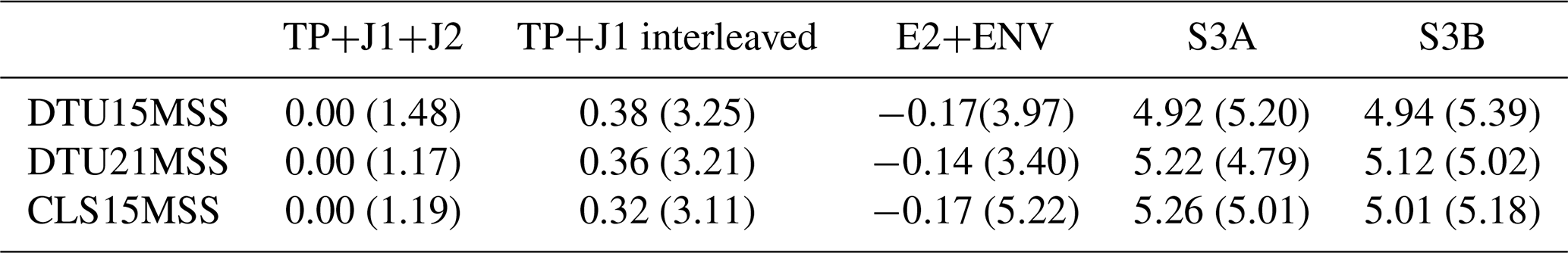
The Sentinel 3A and 3B mean profiles are independent of existing MSS models, but only 66 and 40 cycles have been used, respectively. In the comparison with the Sentinel 3A and 3B mean profiles, we limited the comparison to within the 65^∘ parallels. For all comparisons, the number of repeat cycles can be seen through increased standard deviation with decreasing number of repeat cycles. This illustrates the effect of natural variability of the sea surface and how this is gradually averaged out with an increasing number of repeats. The roughly 5 cm mean difference between S3A and 3B mean profiles and the MSS models directly illustrates the effect of global sea-level rise during the altimetric era. A measurement of 5 cm roughly corresponds to the well-known 3 mm yr⁻¹ sea-level rise accumulated between the center period of January 2003 for the MSS and the averaging period of S3A and 3B some 15 years later. All comparisons indicate that the DTU21MSS performs slightly superiorly compared with all older models.

3.2 Arctic evaluation

Within the ESA Cryo-TEMPO project, we evaluated the impact of the use of a physical retracker and an empirical retracker on the retrieval of sea-level anomalies in the polar ocean. We used the state-of-the-art empirical retracker called the Threshold First Maximum Retracker Algorithm (TFMRA) (Helm et al., 2014) and the SAMOSA+ physical retracker. In the evaluation, we also compared the state-of-the-art MSS models, the DTU15MSS and DTU21MSS. It was not possible to include the CLS15MSS as this model only covers up to 84^∘ N and has several voids in the Arctic Ocean (Pujol et al., 2017). The use of the physical retracker allows us to estimate the sea state bias (SSB). This sea state bias correction was subsequently applied to both the SAMOSA+ physical SLA and the empirical TFMRA SLA.

A total period of 7 months of Cryosat-2 was used between October 2013 and April 2014. The results are shown in Fig. 6, where the upper panels show the spatial variation in the mean (two left panels for the TFMRA and SAMOSA+ retracked SLA) and the corresponding standard deviation of SLA (two right panels). The lower panels highlight the time evolution of the monthly SLA anomalies averaged with the monthly mean given in the left panel and the standard deviation given in the right panel.

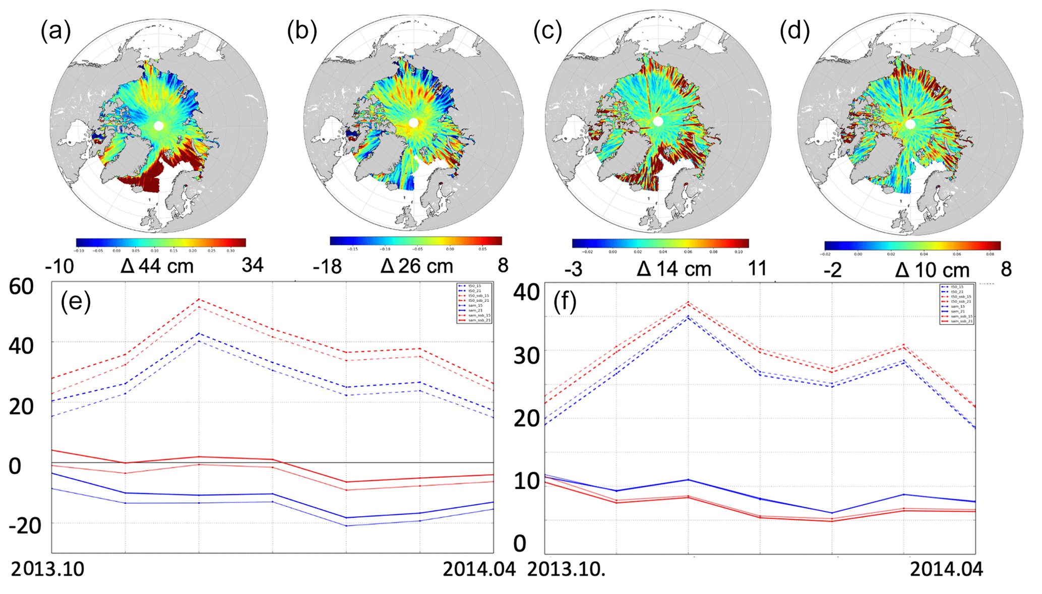
Figure 6 Comparison of retrackers and MSS models over the Arctic Ocean from October 2013–April 2014. Upper panels: mean SLA using the empirical TFMRA retracker and the DTU15MSS (a) and mean SLA using SAMOSA+ and the DTU21MSS (b). The standard deviation of SLA using the empirical TFMRA retracker and the DTU15MSS (c) and standard deviation of SLA using SAMOSA+ and the DTU21MSS (d). Lower panels: evolution of SLA in time. The mean (e) and standard deviation (f) are shown as monthly values. Heavy lines correspond to using DTU21, and thin lines correspond to using DTU15. The dotted lines correspond to using the TFMRA retracker and the solid lines to the SAMOSA+ retracker. The red lines have the sea state bias correction applied, whereas the blue lines have not.

This study shows an improved measurement of SLA using the physical SAMOSA+ retracker, and in all cases, the DTU21MSS delivers better results than the DTU15MSS. When using the physical SAMOSA+ retracker, we can see that there is a clear effect of the ability to determine and correct for the sea state bias (SSB). With SAMOSA+ sea state bias applied referenced to the DTU21MSS, we obtain a mean SLA of $-\mathrm{1.5}\mathrm{cm}\pm \mathrm{12}\mathrm{cm}$ instead of $-\mathrm{5.4}\mathrm{cm}\pm \mathrm{22}\mathrm{cm}$ over the October 2013–April 2014 period when using an empirical retracker and the DTU15MSS.

To illustrate the difference between various MSS models across the Arctic Ocean, we computed the difference between the DTU21MSS and the DTU15MSS and CLS15MSS, respectively.

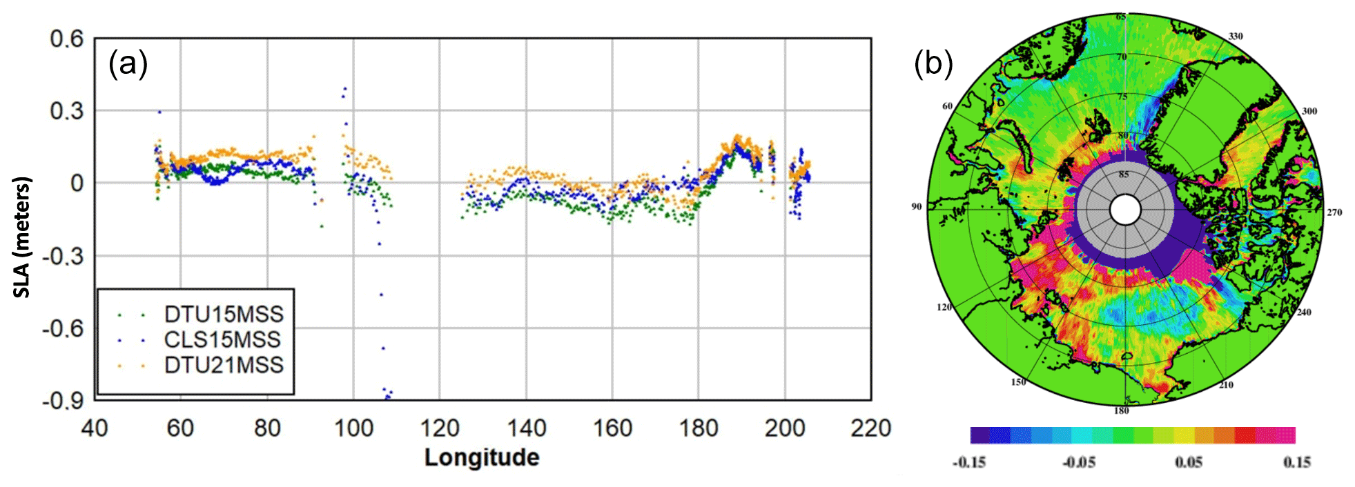
Figure 7 Sea-level anomalies (in m) between the 5-year S3A mean profile along track 497–498 and various MSS models in the Arctic Ocean (a). (b) Mean sea surface difference between the DTU21MSS and the CLS15MSS dark-blue regions north of Canada are voids in the CLS15MSS. The color scale ranges from −15 to +15 cm.

To illustrate the differences between the various MSS models, we computed the difference between a Sentinel 3A 5-year mean profile and the various MSS models. Figure 7 shows this difference along the Sentinel 3A track 497–498. The track transits from Russia at 68^∘ N, 54^∘ E, passing to the east of Novaya Zemlya, and continues up to 82^∘ N (at 120^∘ E). From here it descends towards the Aleutian Trench at 57^∘ N, 204^∘ E. The standard deviations with the S3A mean profiles are 6.1, 5.7 and 8.1 cm respectively for the DTU15MSS, DTU21MSS and CLS15MSS. Data are missing around latitude 90^∘ E because of the crossing of the Russian island of Komsomolets. Data are missing around 120^∘ E because of voids in the CLS15MSS causing the S3A data to be removed by the space agencies. The color scale ranges from −15 to +15 cm. The increase in the S3A residuals around 190^∘ E is associated with the transition of the Bering Strait and the in- and outflow through the strait (Woodgate and Peralta-Ferriz, 2021).

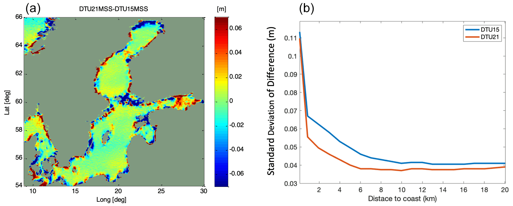
Figure 8 Difference between the DTU21MSS and the DTU15MSS in the Baltic Sea (a). Standard deviation (m) relative to the Danish vertical reference model, DVR90, as a function of distance to coast (b).

3.3 Coastal evaluation

The difference between the DTU21MSS and the DTU15MSS was evaluated in the Baltic Sea as part of the Baltic+ SEAL project (http://balticseal.eu/, last access: 25 August 2023). Differences are presented in Fig. 8 (left) panels and range up to 8 cm in the coastal zone and inside the narrow Danish Straits as well as the Bay of Bothnia and the Swedish archipelago. In all locations, we found that the former DTU15MSS is unreasonably high near the coastline. Around the coast of Denmark, we further compared with the vertical reference frame model of Denmark called DVR90 (Web2, 2023). DVR90 is fitted to 14 Global Navigation Satellite System (GNSS) stations along the coastline of Denmark. The right panel illustrates that the DTU21MSS has a lower standard deviation close to the coast compared with the DTU15MSS, which independently verifies that the DTU21MSS is superior in fitting mean sea level close to the coast.

4 Data availability

The DTU21MSS is available from https://doi.org/10.11583/DTU.19383221.v1 (Andersen, 2022). The high-resolution MSS model is available in several formats and relative to various reference ellipsoids (TOPEX and WGS84) https://doi.org/10.11583/DTU.19383221.v1 (Andersen, 2022).

5 Conclusions

A new mean sea surface (MSS) called DTU21MSS for referencing sea-level anomalies from satellite altimetry has been presented, along with the first evaluations. We have presented the updated processing chain with updated editing and data filtering. The updated processing filters the double retracked 20 Hz sea surface height data using the Parks–McClellan filter to derive 2 Hz sea surface anomaly. This Parks–McClellan filter has a clear advantage over the 1 Hz boxcar filter used for older DTU models in enhancing the MSS in the 10–40 km wavelength band. Similarly, the use of the FES2014 ocean tide model improves the usage of sun-synchronous satellites in high latitudes in the new MSS.

Cryosat-2 employs SAR and SARin modes in a large part of the Arctic Ocean due to the presence of sea ice. For SAR- and SARin-mode data we applied the SAMOSA+ physical retracking (Dinardo et al., 2018) to make it compatible with the physical retracker used for conventional low-resolution-mode data in other parts of the global ocean.

We initially performed global comparisons with the mean profile from various available satellites using data from the RADS data archive as these have only been used in the DTU15MSS and not any of the other MSS models. The comparison with the independent 5- and 3-year S3A and S3B mean profiles show a relatively clear improvement for the DTU21MSS. This was also expected as the S3A and 3B satellites employs SAR altimetry and hence should compare better with the MSS derived using the two-pass altimetry due to the enhanced modeling of the 10–30 km wavelength (Garcia et al., 2013).

The evaluation in the Arctic Ocean indicates an improved measurement of SLA using SAMOSA+ with the DTU21MSS. In conjunction with this physical retracker, the correction of the sea state bias (SSB) further improves the results. In all evaluations, the DTU21MSS delivers better results than the DTU15MSS. With SAMOSA+, SSB and the DTU21MSS, we obtain a mean SLA of $-\mathrm{1.5}\mathrm{cm}\pm \mathrm{12}\mathrm{cm}$ instead of $-\mathrm{5.4}\mathrm{cm}\pm \mathrm{22}\mathrm{cm}$ over the October 2013–April 2014 period.

Coastal evaluation of the new DTU21MSS was performed in the Baltic Sea. The evaluation in the Baltic Sea confirms that the DTU15MSS is frequently several centimeters too high in the coastal zone. This was further demonstrated in an evaluation with the Danish Vertical Reference model based on GNSS observations, where the DTU21MSS showed superior comparison close to the coast.

For the DTU21MSS we found that the 5-year Sentinel 3A mean profiles (May 2016–May 2020) were too problematic to consolidate onto the 1993–2012 averaging period without degrading the MSS model, particularly in large current regions. Consequently we omitted these data in the DTU21MSS but also found that we will need to extend the averaging period to 30 years soon to enable the use of the important new Sentinel 3A and 3B data in the next-generation MSS models.