High-resolution land use and land cover dataset for regional climate modelling: historical and future changes in Europe

Anthropogenic land use and land cover change (LULCC) is a major driver of environmental changes. The biophysical impacts of these changes on the regional climate in Europe are currently being extensively investigated within the World Climate Research Program (WCRP) Coordinated Downscaling Experiment (CORDEX) Flagship Pilot Study (FPS) Land Use and Climate Across Scales (LUCAS) using an ensemble of different regional climate models (RCMs) coupled with diverse land surface models (LSMs). In order to investigate the impact of realistic LULCC on past and future climates, high-resolution datasets with observed LULCC and projected future LULCC scenarios are required as input for the RCM–LSM simulations. To account for these needs, we generated the LUCAS Land Use and land Cover change (LUC) dataset version 1.1 at 0.1^∘ resolution for Europe with annual LULC maps from 1950 to 2100 (https://doi.org/10.26050/WDCC/LUC_hist_EU_v1.1, Hoffmann et al., 2022b, https://doi.org/10.26050/WDCC/LUC_future_EU_v1.1, Hoffmann et al., 2022a), which is tailored to use in state-of-the-art RCMs. The plant functional type (PFT) distribution for the year 2015 (i.e. the Modelling human LAND surface Modifications and its feedbacks on local and regional cliMATE – LANDMATE – PFT dataset) is derived from the European Space Agency Climate Change Initiative Land Cover (ESA-CCI LC) dataset. Details on the conversion method, cross-walking procedure, and evaluation of the LANDMATE PFT dataset are given in the companion paper by Reinhart et al. (2022b). Subsequently, we applied the land use change information from the Land-Use Harmonization 2 (LUH2) dataset, provided at 0.25^∘ resolution as input for Coupled Modelling Intercomparison Project Phase 6 (CMIP6) experiments, to derive LULC distributions at high spatial resolution and at annual time steps from 1950 to 2100. In order to convert land use and land management change information from LUH2 into changes in the PFT distribution, we developed a land use translator (LUT) specific to the needs of RCMs. The annual PFT maps for Europe for the period 1950 to 2015 are derived from the historical LUH2 dataset by applying the LUT backward from 2015 to 1950. Historical changes in the forest type changes are considered using an additional European forest species dataset. The historical changes in the PFT distribution of LUCAS LUC follow closely the land use changes given by LUH2 but differ in some regions compared to other annual LULCC datasets. From 2016 onward, annual PFT maps for future land use change scenarios based on LUH2 are derived for different shared socioeconomic pathway (SSP) and representative concentration pathway (RCP) combinations used in the framework of CMIP6. The resulting LULCC maps can be applied as land use forcing to the new generation of RCM simulations for downscaling of CMIP6 results. The newly developed LUT is transferable to other CORDEX regions worldwide.

1 Introduction

Human land surface modifications through land use are an important forcing on climate, and their direct biophysical effects on the local and regional climate can be as large as those associated with global greenhouse gas forcing (de Noblet-Ducoudré et al., 2012). Land use and land cover change (LULCC) affects land–atmosphere processes through modifications of the surface energy balance (Mahmood et al., 2014; de Noblet-Ducoudré and Pitman, 2021). Up to now, LULCC forcing has not been sufficiently accounted for in climate change projections conducted with regional climate models (RCMs), although the strongest impact of LULCC is found especially at those finer regional scales (Mahmood et al., 2014; Davin et al., 2014). Thus, robust fine-scale LULCC reconstructions are needed to quantify the interaction between regional and local biogeochemical and biophysical processes within RCMs, which may support effective land-use-based climate adaptation and mitigation measures.

The first coordinated downscaling experiments including land use changes were performed in the framework of the World Climate Research Program (WCRP) Coordinated Downscaling Experiment (CORDEX) Flagship Pilot Study (FPS) Land Use and Climate Across Scales (LUCAS) (Rechid et al., 2017). An ensemble of different RCMs coupled to diverse land surface models (LSMs) has been set up to perform idealized experiments with extreme LULCC scenarios for the EURO-CORDEX domain at 0.44^∘ resolution (EUR-44) driven by ERA-Interim reanalysis. The responses of the RCM–LSM ensemble to the two extreme LULCC scenarios show robust seasonal temperature signals for some regions and variables but disagreement for others between the different RCMs and LSMs originating mainly from the different representations of land processes in the models (Davin et al., 2020; Breil et al., 2020).

In the next phases of LUCAS and within the Coordinated Downscaling Experiment – European Domain (EURO-CORDEX) (Jacob et al., 2020), plans exist to conduct simulations with past and future LULCC forcings at a ∼ 12.5 km (i.e. the EURO-CORDEX domain at 0.11^∘ resolution, EUR-11, domain) horizontal resolution. For some specific sub-regions in Europe, simulations will also be carried out at convection-permitting resolutions. This approach implies new requirements for LULCC reconstructions and scenarios.

1. A high spatial resolution (1 km or below) exists over an extent that covers the entire EURO-CORDEX domain in order to enable the investigation of LULCC impacts on small-scale processes such as local wind systems, convection, boundary layer processes, and scale interactions (Mahmood et al., 2014).

2. The temporal coverage starts from 1950, which is the time frame defined in the EURO-CORDEX historical experiments. Further, the LULCC product should extend until 2100 to analyse the impact of several shared socioeconomic pathway (SSP) and representative concentration pathway (RCP) scenarios accounting for changes to both anthropogenic emissions and LULCC.

3. A LULCC forcing must be generally consistent with the LULCC forcing employed by the driving global climate models or Earth system models (GCMs or ESMs), as is the case for other forcing data such as greenhouse gas or aerosol emissions (Taranu et al., 2023; Wohland, 2022).

4. A choice of land use and land cover classes must match the specific needs of current RCMs. For instance, at scales of ∼ 50 km and lower, urban land cover plays an important role (Chapman et al., 2019; Daniel et al., 2019; Katzfey et al., 2020) and should be represented. Moreover, at these scales the ratio of needleleaf to broadleaf trees becomes a meaningful aspect to consider (Naudts et al., 2016; Schwaab et al., 2020). Finally, land management practices such as irrigation significantly alter local and regional climate and are implemented in RCMs (Lobell et al., 2009; Valmassoi et al., 2020; Asmus et al., 2023). Thus, irrigation changes should be accounted for in the reconstruction and scenarios.

The LULCC reconstructions applied within the Coupled Model Intercomparison Project Phase 6 (CMIP6; Eyring et al., 2016) and the Land Use Model Intercomparison Project (LUMIP; Lawrence et al., 2016) are harmonized with future projections based on SSP and RCP scenarios in order to generate the Land-Use Harmonization 2 dataset (LUH2; Hurtt et al., 2020). These land use and land management changes are available from 850 until 2100 (with extension until 2300) on a global 0.25^∘ grid. Thus, LUH2 meets the requirement for the length of the dataset but not for spatial resolution. In addition, the land use classes do not correspond to land use and land cover classes employed in most GCMs or RCMs.

Consequently, many modelling groups will have to convert the LUH2 land use changes into changes in land cover and land use input prior to their use in GCMs. For this conversion, so-called land use translators (LUTs) are applied (e.g. Di Vittorio et al., 2014; Mauritsen et al., 2019; Lurton et al., 2020) that are usually model-specific. For most GCMs and ESMs, LUTs only account for changes in land use classes such as cropland, pasture, rangeland, and natural vegetation (e.g. Mauritsen et al., 2019; Lurton et al., 2020). Within the natural vegetation class the relative distribution of vegetation types such as forest, shrubs, or grassland is constant or computed by the dynamic vegetation model despite the fact that LUH2 provides information on changes in forested and non-forested vegetation. Keeping the relative proportion of land cover types constant in the natural fraction of the land in RCMs, which do not include dynamic vegetation models, would be a major limitation and would not meet the requirements listed above. In addition, urban changes are mostly discarded in LUT approaches because urban land use is not considered by most GCMs, with some exceptions (e.g. Jackson et al., 2010; Danabasoglu et al., 2020; Katzfey et al., 2020). Consequently, we developed a new LUT approach, which also accounts for changes in the distribution of natural vegetation types and urban areas, and generated a new land cover input dataset for RCMs that is consistent with the LUH2 dataset, which is also used in CMIP6.

Inconsistencies due to the coarse resolution of LUH2 are tackled to a large extent by applying the LUT to a high-resolution initial land cover dataset. There is a wide range of observed high-resolution land cover datasets available that have been used to generate land cover input for RCMs, e.g. Coordination of Information on the Environment (CORINE), MODIS, ESA-CCI LC, Global Land Cover Map (GlobCover), or HIstoric Land Dynamics Assessment + (HILDA+). However, some of these datasets are only available for certain regions, such as CORINE (Jaffrain et al., 2017), which is only available for European countries. Within CMIP6 GCMs and ESMs, the ESA Climate Change Initiative Land Cover product (ESA-CCI LC; ESA, 2017) is increasingly being applied. ESA-CCI provides a LC time series including annual maps from 1992 to 2018 on a global ∼ 300 m grid, a resolution suitable for kilometre-scale RCM simulations. The dataset shows good agreement with other land cover products, globally and regionally (Achard et al., 2017; Reinhart et al., 2021). In addition, ESA-CCI LC has already been used for RCM studies on the impact of LULCC on the climate in Europe (Huang et al., 2020), where the potential for the use of this dataset for RCMs was demonstrated. Reinhart et al. (2022b) developed a workflow to convert the ESA-CCI LC land cover classes into plant functional types (PFTs) as well as non-vegetated classes such as urban and bare ground for the European domain. The resulting Modelling human LAND surface Modifications and its feedbacks on local and regional cliMATE (LANDMATE) PFT dataset (version 1.1) (Reinhart et al., 2022a) shows good agreement with ground truth observations and thus provides the initial land cover map for the LUT approach.

In this study, we introduce the new high-resolution, historical, and future LUCAS Land Use and land Cover change (LUC) dataset (version 1.1) (Hoffmann et al., 2022b, a), which we prepared to meet the requirements for the next-generation RCM simulations for downscaling CMIP6 by the EURO-CORDEX community and in the framework of FPS LUCAS.

2 Methods and datasets

2.1 Workflow to generate the LUCAS LUC dataset

The workflow to generate the LUCAS LUC dataset is shown in Fig. 1. It starts with the generation of a PFT map based on the ESA-CCI LC dataset, the so-called LANDMATE PFT dataset (Sect. 2.2.1). The methods and datasets used to create this dataset are described in the companion paper by Reinhart et al. (2022b). Therefore, only a short description of the base-map development is given in this paper. First, the ESA-CCI LC map for the year 2015, which has a native resolution of ∼ 300 m, is aggregated to 0.1^∘ resolution using the SAGA GIS tool Coverage of Categories (Conrad et al., 2015). It computes the percentage of each ESA-CCI LC class within $\mathrm{0.1}{}^{\circ }\times \mathrm{0.1}{}^{\circ }$ grid cells. Thereafter, the aggregated ESA-CCI LC map is converted into a set of PFTs. For the conversion of the ESA-CCI LC land cover classes into PFTs, a cross-walking procedure is commonly applied (Wilhelm et al., 2014; Li et al., 2018; Georgievski and Hagemann, 2019; Lurton et al., 2020; Reinhart et al., 2022b). Therefore, for each ESA-CCI LC land cover class, we set up a so-called cross-walking table (CWT), which defines the composition of this class in terms of PFT fractions. The CWTs are further refined based on climate zones defined through the Holdridge life zones (HLZs; Wilhelm et al., 2014). The HLZ concept proposes a global classification of climatic zones in relation to potential vegetation cover dependent on mean annual precipitation data and mean monthly temperature (Holdridge, 1967). Supported by the HLZs, it is possible to customize the CWT for each ESA-CCI LC class in a way that fits the respective climate region, which is of special importance when translating mixed vegetation classes into PFTs. The HLZs for the European domain are computed from atmospheric observations of temperature and precipitation taken from the E-OBS dataset and the CRU dataset (outside the geographical range of E-OBS). Using the higher-resolution E-OBS dataset (0.1^∘ resolution) instead of the rather coarse CRU dataset (0.5^∘ resolution), as was done by Wilhelm et al. (2014), allows for a more detailed representation of HLZs, especially in regions with complex terrain. The distribution of C₃ and C₄ grasses within grassland areas, distinguished by some LSMs, is taken from a separate potential C₄ map provided by the North American Carbon Program (NACP) for the Multi-scale Synthesis and Terrestrial Model Intercomparison Project (MsTMIP).

The information needed to compute changes in the PFT distribution is taken from the LUH2 dataset (Sect. 2.2.3), which provides land use states and transitions and land management information on a global 0.25^∘ grid from 850 to 2015 (reconstructed) and from 2016 until 2100 (projected). The land use classes and subsequently the land use transitions mainly represent land used by humans through agriculture, livestock farming, and forest management and only distinguish between forested and non-forested vegetation. Thus, they cannot directly be imposed on the LANDMATE PFTs, which mainly represent the physical land cover.

Instead, the LUH2 land use transitions are translated into annual changes in PFT fractions for the historical period starting in 2015 and going back until 1950 using the newly developed LUT (Sect. 2.3). While LUH2 provides transitions of forest vegetation, historical changes in the forest type distributions are taken from a European forest area and species composition dataset provided by McGrath et al. (2015) (Sect. 2.2.2). By employing the LUT forward in time, the future annual PFT changes are computed from the eight different land use change scenarios provided by LUH2. In special cases, where a certain vegetation type is not present within a grid cell but should be increased according to the LUH2 and the rules provided by the LUT, a background map of potential vegetation is needed. This map is constructed from the ESA-CCI LC dataset and the CWT used for the LANDMATE PFTs (Sect. 2.2.1).

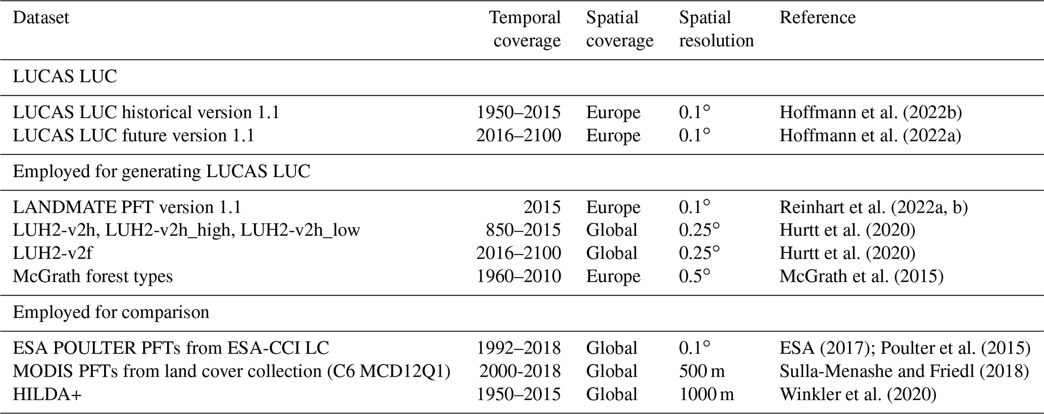
The final LUCAS LUC dataset consists of one file containing the annual PFT maps for the historical period from 1950 until 2015 (Hoffmann et al., 2022b) and eight different files for the land use change scenarios for the future period from 2016 to 2100 (Hoffmann et al., 2022a). For the comparison of the historic land cover changes, the ESA-CCI LC-based PFT time series, the MODIS PFT dataset, and HILDA+ are employed (Sect. 2.5). An overview of the datasets employed in this study is given in Table 1.

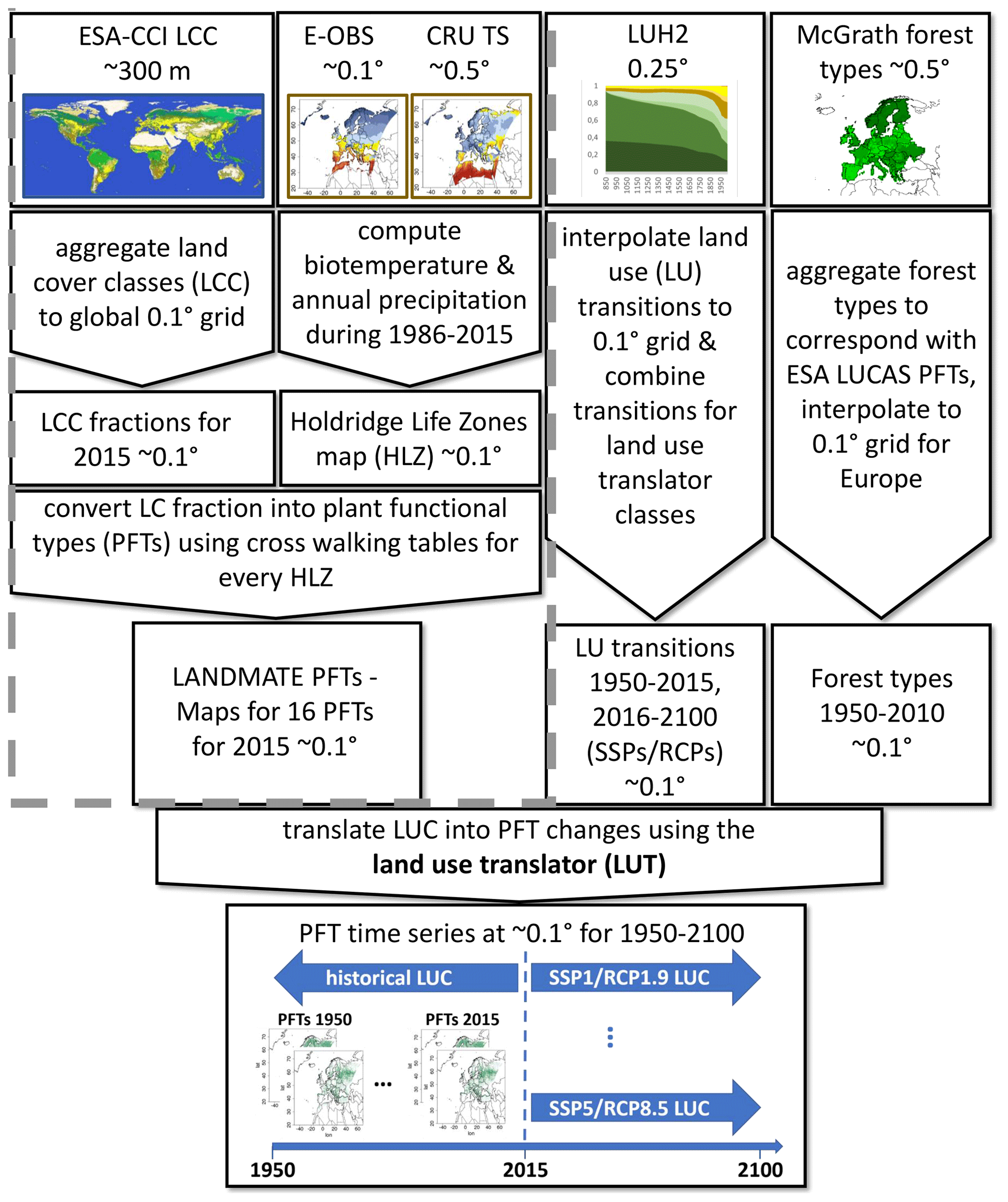
Figure 1 Workflow for generating the LUCAS LUC dataset. The steps and datasets highlighted in the grey dashed box are described in detail by Reinhart et al. (2022b).

Hoffmann et al. (2022b)Hoffmann et al. (2022a)Reinhart et al. (2022a, b)Hurtt et al. (2020)Hurtt et al. (2020)McGrath et al. (2015)ESA (2017); Poulter et al. (2015)Sulla-Menashe and Friedl (2018)Winkler et al. (2020)

Table 1 Datasets employed in the present study.

2.2 Land use and land cover datasets

2.2.1 LANDMATE PFT dataset version 1.1

The LANDMATE PFT dataset version 1.1 for the year 2015 is used as a base map and as a starting point for the land cover changes that are computed with the LUT (Sect. 2.3). Background maps, required for the LUT, are generated depending on the HLZ for the grass, shrub, and tree PFTs, respectively, based on the CWTs described in Reinhart et al. (2022b). For example, the background map for the tree PFT group consists of tree PFT fractions that are most likely to grow given the HLZ for each land point. When applied to other regions, this map would need to be adjusted for the dominant vegetation cover of the region, e.g. for Australia, where temperate broadleaf evergreen forest is one of the dominant forest types.

The distribution of the PFTs in the LANDMATE PFT dataset (a major PFT class per 0.1^∘ grid cell) in 2015 is shown in Fig. 2. In many regions of Europe, cropland is the dominant PFT. In Scandinavia and northern Russia, temperate evergreen forest is dominant, which changes into tundra at higher latitudes and altitudes. Even at a 0.1^∘ resolution, urban land cover is the dominant land cover for a number of grid cells covering the major urban areas (e.g. London, Paris, or the Ruhr area). This emphasizes the importance of including urban areas at resolutions employed in EURO-CORDEX (i.e. ∼ 12.5 km and higher).

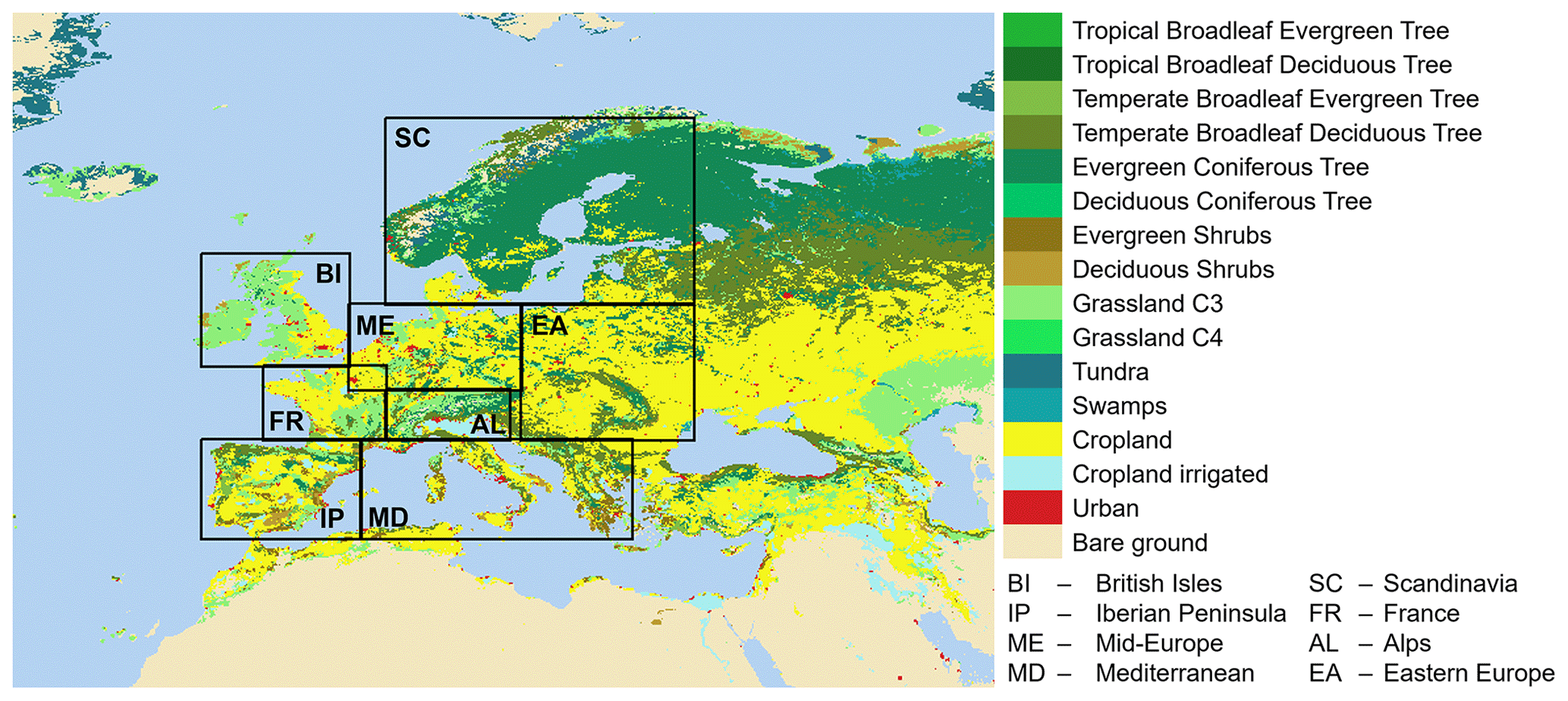
Figure 2 Distribution of the 16 LANDMATE PFTs at 0.1^∘ resolution for 2015 based on ESA-CCI LC. The irrigation map from LUH2 is used to distinguish between irrigated crops and rainfed crops. For improved visualization, the majority PFT is shown.

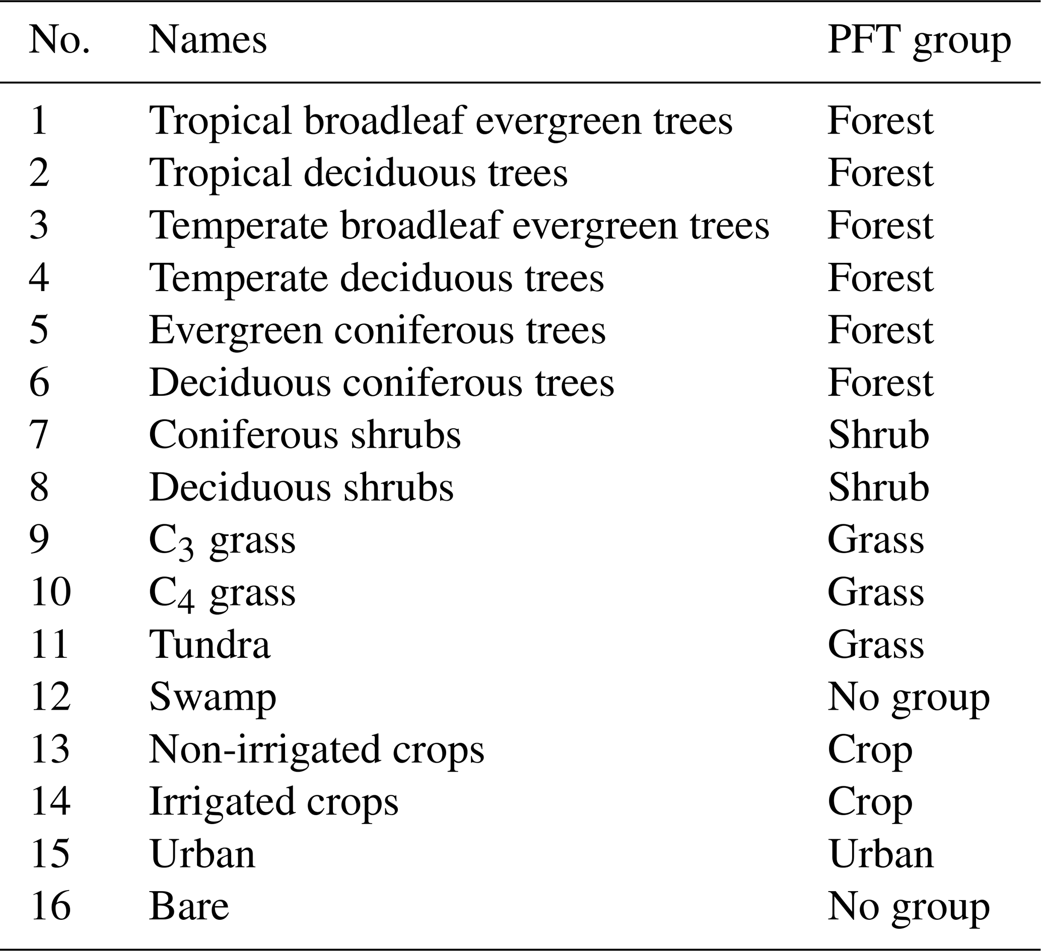
Table 2 LANDMATE PFTs and non-vegetated classes based on Reinhart et al. (2022b). In addition, the grouping used within the LUT (Sect. 2.3) is given (i.e. the PFT group).

2.2.2 European forest area and species composition

The dataset from McGrath et al. (2015) provides tree species composition on a 0.5^∘ grid for Europe from 1600 to 2010, taking into account the conversion of tree species due to forest management. The forest area was reconstructed based on the tree species maps of Brus et al. (2012), the land cover map of Poulter et al. (2015), and the historical land use maps of Kaplan et al. (2012, 2009). A detailed description of the tree species dataset is given by Naudts et al. (2016). While in Naudts et al. (2016) Larix sp. (the only deciduous coniferous species present in the dataset) is listed as a tree species, the fractions for this species are zero in the dataset. Consequently, no additional information for the time evolution is available for the deciduous coniferous PFT. The allocation of the tree species to the remaining three tree PFTs is provided in Table 3.

Table 3 Allocation of the tree species data (McGrath et al., 2015; Naudts et al., 2016) to the tree PFTs. Please note that Naudts et al. (2016) classified the needleleaf species as temperate and boreal, even if they are the same species.

2.2.3 LUH2

LUH2 (Hurtt et al., 2020) provides annual land use states and transitions for 12 land use types (7 main land use types and 5 crop types, Table 4) on a global 0.25^∘ regular grid from 850 until 2100, with an extension to 2300 (the LUH2-v2h dataset for the historic time period 850–2015 and the LUH2-v2f dataset for the future time period starting in 2016). In addition, LUH2 provides agricultural management information such as irrigation and fertilization. For the historical period 850–2015, land use changes are based on the History Database of the Global Environment version 3.2 (HYDE3.2; Klein Goldewijk et al., 2017). In addition to the standard dataset, LUH2 provides two historical reconstructions (LUH2-v2h_high and LUH2-v2h_low) in order to provide uncertainty estimates for agricultural areas and wood harvesting taken from the HYDE3.2 dataset. For LUH2-v2h_high, high historical estimates for crop, pasture, and wood harvest compared to LUH2-v2h are assumed, whereas for LUH2-v2h_low, low estimates are assumed (Lawrence et al., 2016; Hurtt et al., 2020).

Future land use changes are based on the output of different integrated assessment models (IAMs) for selected marker SSP–RCP scenarios, of which the most important characteristics are summarized in Table A2. The Global Land Use Model (GLM2; Hurtt et al., 2006, 2011) is employed to translate the land use change information into fractional changes in the land use classes for each $\mathrm{0.25}{}^{\circ }\times \mathrm{0.25}{}^{\circ }$ grid cell using additional datasets and assumptions as constraints. For three scenarios (i.e. SSP1–RCP1.9, SSP1–RCP2.6, and SSP2–RCP4.5), an additional dataset is provided that takes into account the future forestation that is present in these scenarios but was not captured in the initial LUH2 dataset (Hurtt et al., 2020). The dataset contains the variable “added tree cover”, which is the fraction of the $\mathrm{0.25}{}^{\circ }\times \mathrm{0.25}{}^{\circ }$ grid cell that should be converted from non-forested vegetation to forested vegetation to obtain the correct proportion of future forest cover.

2.3 Translating land use changes into PFT changes

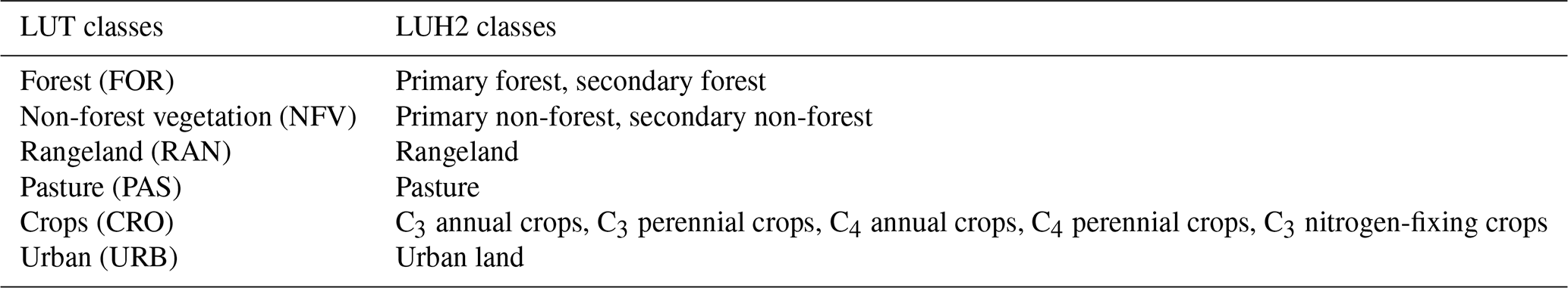
In order to convert the land use change information given by LUH2 into PFT changes, an algorithm with a fixed set of transition rules is developed (Tables 5 and 6). In the first step, LUH2 classes are grouped into the main land use classes, denoted here as LUT classes (Table 4): crops (CRO), forest (FOR), non-forest vegetation (NFV), rangeland (RAN), pasture (PAS), and urban (URB). For these LUT classes the transitions provided by the LUH2 dataset are aggregated. The aggregated transitions are bilinearly interpolated for the 0.25^∘ grid to the 0.1^∘ grid also used for the PFT maps derived from ESA-CCI LC (i.e. the LANDMATE PFT dataset; Sect. 2.2.1), which represent the land cover distribution for the year 2015.

Table 4 Land cover classes used for the land use translator and their corresponding LUH2 land use classes.

The transition rules are defined to ensure that the changes in cropland are as close to the LUH2 changes as possible. In contrast to other LUTs, urban transitions are included. Following the recommendations by Ma et al. (2020) and Hurtt et al. (2020), natural vegetation (i.e. forest and shrubland) is cleared and converted into grassland only for land use transitions to pasture, while it remains unchanged for land use transitions from non-forested vegetation to rangeland. Hence, it is assumed that vegetation is cleared if the land is converted into managed pasture, while it remains unchanged if rangeland is established. An exception to this general rule is the transition from forest to rangeland when the land will be used for livestock grazing.

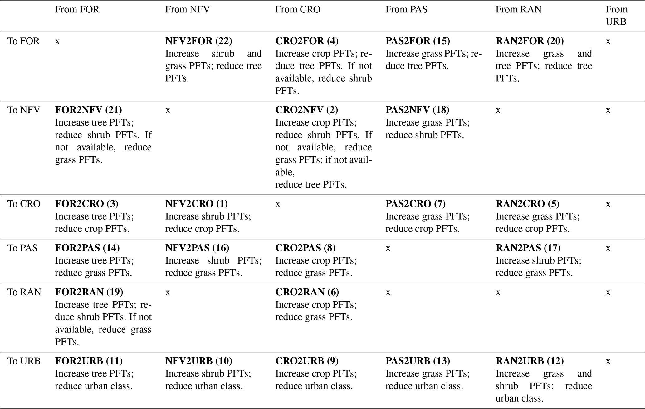
The PFTs are increased or reduced according to the rules given in Tables 5 and 6. The transitions are computed sequentially according to the numbering in Tables 5 and 6. The forward translation starts with transitions from and to cropland, followed by urban transitions. Thereafter, the remaining pasture and rangeland transitions are computed. Transitions from forest to non-forested vegetation (i.e. shrubland and grassland) and vice versa are not considered in the forward translation because these fields are zero in the original LUH2 scenario data. Consequently, future afforestation and deforestation only occur if land use transitions related to the land use classes urban, cropland, rangeland, and pasture are present. An exception is made for the three scenarios SSP1–RCP1.9, SSP1–RCP2.6, and SSP5–RCP4.5, where a separate dataset is provided for afforestation (Sect. 2.3.2). The backward translation also starts with cropland and urban transitions. Since the historical transitions from urban to any other LUH2 land use class are zero, these are not listed in Table 6. The backward translation continues with the pasture and rangeland transitions.

Since the vegetation fractions differ between the LANDMATE PFT map, used as the base map for LUCAS LUC, and LUH2 (e.g. the spatial distribution of the forest fraction), the rules are designed to be flexible. In order to ensure that crop and urban changes are as close as possible to the changes provided by LUH2, transitions to crops are not as strict regarding the treatment of the PFTs that occupied the grid cell previously. For example, during the transition of forest to cropland (FOR2CRO in Table 5), the LUT checks whether enough tree PFTs are available. If this is not the case, shrub PFTs are reduced and in a subsequent step also the grass PFTs, given that the sum of forest and shrub PFTs is still smaller than the transitions. The reduction of a PFT group is done until its fraction is zero.

For each transition in Tables 5 and 6, the relative PFT fractions remain constant within each PFT group (Table 2). For example, an increase in non-forest vegetation would lead to an increase in all shrub and grass PFTs that are present within a grid cell. If a PFT class (e.g. tree PFTs) is not present in a certain grid cell but is supposed to increase, the relative fractions for this class are taken from the corresponding background map (Sect. 2.2.1). Bare ground and swamps remain unchanged because there is no information on bare-ground or wetland changes in the LUH2 dataset and there is no additional information available that could justify a conversion of bare ground or wetlands to vegetation or crops or vice versa. Hence, land cover changes related to desertification, cropland expansion into the desert, and drainage of wetlands are not included in the LUCAS LUC dataset.

2.3.1 Accounting for historical forest type distribution

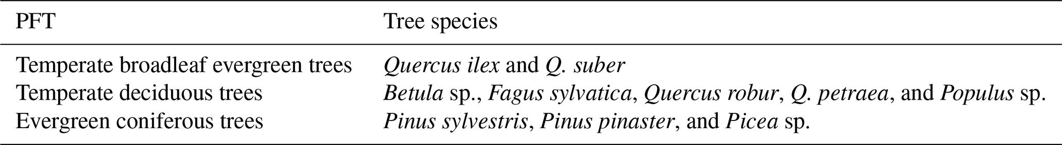
For the backward extension of historical forest type distribution, additional information on the relative distribution of broadleaf and needleleaf forest taken from the McGrath dataset is employed (Sect. 2.2.2). To avoid alteration of the base map derived from ESA-CCI LC, the relative fractions of three tree types (temperate broadleaf evergreen trees, temperate deciduous trees, evergreen coniferous trees) are not directly imposed on the PFT maps. Instead, only the trend in the relative fraction is used. For every time step the differences in the relative fractions of the three PFTs are computed. These relative fraction changes are then converted into fraction changes of the individual PFTs by multiplying the relative fraction changes by the sum of the three PFTs.

2.3.2 Adding tree cover for future scenarios

For the three scenarios SSP1–RCP1.9, SSP1–RCP2.6, and SSP5–RCP4.5, respectively, an additional transition is computed because the afforestation signal is not correctly captured in the LUH2 land use transitions (Hurtt et al., 2020). After the computation of transitions provided by LUH2 projections, the tree PFTs are increased by employing the added tree cover data (Sect. 2.2.3). Here, the same rules as for the transitions from forested vegetation to non-forested vegetation in the backward translation are applied (FOR2NFV in Table 6), increasing tree PFTs and reducing non-forested PFTs, starting with shrub PFTs and, if their fraction is reduced to zero, grass PFTs.

2.3.3 Treatment of irrigated cropland

After the translation procedure, irrigated and non-irrigated crops are separated based on the irrigation fractions (e.g. irrigation of C₃ annual crops) for the different crop classes provided by LUH2. These fractions are aggregated to create a single irrigation fraction per grid cell. Within the irrigation fraction there is no consistent information on the irrigation practice (e.g. sprinkler or channel irrigation) available. After each transition time step of 1 year, the crop PFTs are summed up and multiplied by the irrigation fraction and (1 − irrigation fraction), respectively.

Table 5 LUT rules for the translation of LUT class changes into PFT changes forward in time using the LUT classes given in Table 4 and the PFT group definitions given in Table 2. This means that the transitions refer to the changes in the PFT fraction from time step t to time step t+1. Transitions between LUT classes are bold. Transitions not used within the LUT are denoted with an “x”.

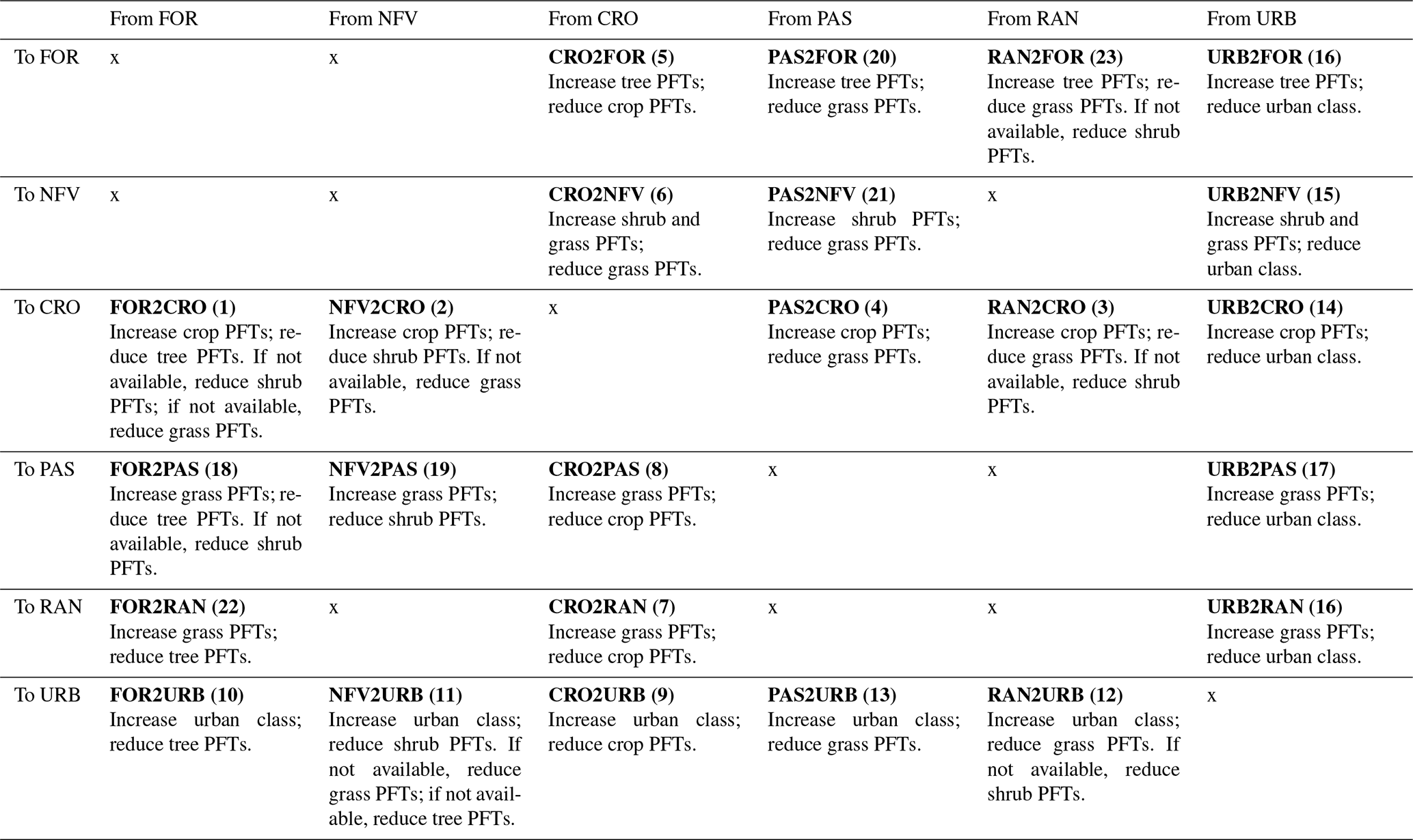
Table 6 LUT rules for the translation of LUT class changes into PFT changes backward in time using the LUT classes given in Table 4 and the PFT group definitions given in Table 2. Please note that the transitions provided by LUH2 are the same as in Table 5, but the changes in PFTs given in this table are imposed backward in time. This means that the transitions refer to the changes in the PFT fraction from time step t to time step t−1. Transitions between LUT classes are bold. Transitions not used within the LUT are denoted with an “x”.

2.4 Uncertainty measures

To account for the main uncertainties of the historical LULCC, two different historical reconstructions have been provided, the so-called LUH2-v2h_low and LUH2-v2h_high datasets (Sect. 2.2.3). They are in turn based on the uncertainty estimates of the HYDE3.2 dataset for the population data and for the cropland and grazing land cover.

In order to quantify the uncertainty in the LUCAS LUC dataset for the historical period, the LUCAS LUC dataset has been generated using the three different LUH2 reconstructions (i.e. historical, historical high, and historical low) and at 0.1^∘ resolution and the native resolution of the LUH2 dataset (0.25^∘). From these six datasets (three reconstructions per resolution), two measures were derived. Following Winkler et al. (2021), the uncertainty is defined as the spread of a given PFT in a grid cell. Consequently, changes can be defined as robust if their absolute values are larger than the spread. As an aggregated measure of robustness, the fraction of robust changes for a given PFT or land cover category and a given region, i.e. the ratio of robust changes to all changes, is used. For the computations, only fraction changes of 0.01 (i.e. 1 % of the grid cell) and larger are considered.

The second measure is the agreement on the sign of the change, which is a widely used measure for the robustness of changes in climate research. For each of the six datasets, the changes in PFTs are computed with respect to their base map for the year 2015. The measure is 1 if all of the datasets show the same direction of changes (i.e. all decrease or all increase) and 0 otherwise. It is used for generating the historical land cover change maps (Figs. 3 and 6) in this paper.

2.5 Comparison with existing LULCC datasets

In addition to the uncertainty analysis, the historical trends of LUCAS LUC PFTs are compared to the trends in the ESA-CCI-based PFT time series (i.e. ESA POULTER, Sect. 2.5.1), the MODIS PFT time series (Sect. 2.5.2), and the land use change dataset HILDA+ (Sect. 2.5.3). The land use states (LUH2), land use classes (HILDA+), and PFTs (MODIS, LUCAS LUC, and ESA POULTER) are aggregated to the land cover groups cropland, grassland, forest, and urban according to Table 7. Note that for this purpose the LUH2 land use class pasture is assigned to grassland because LUH2 does not provide a grassland type and that only the classes urban, cropland, and forest are taken from HILDA+ because no distinction between shrubs and grassland was made for this dataset. The spatial extent of the land cover fraction changes (Fig. 3) between 1992 and 2015, the period covered by ESA POULTER, and the time series of aggregated area changes (Fig. 4) are investigated. For the latter analysis, land cover fractions are converted into area coverage per year for eight European sub-regions defined within the project Prediction of Regional scenarios and Uncertainties for Defining EuropeaN Climate change risks and Effects (PRUDENCE; Christensen et al., 2007; Christensen and Christensen, 2007; Fig. 2), taking into account the land–sea mask from ESA POULTER, which is the same for LUCAS LUC. Results will be shown for IP (Iberian Peninsula), ME (Mid-Europe, and EA (Eastern Europe) and discussed as these regions are representative for illustrating the strengths and weaknesses of the high-resolution LULCC reconstruction (Sect. 3.1).

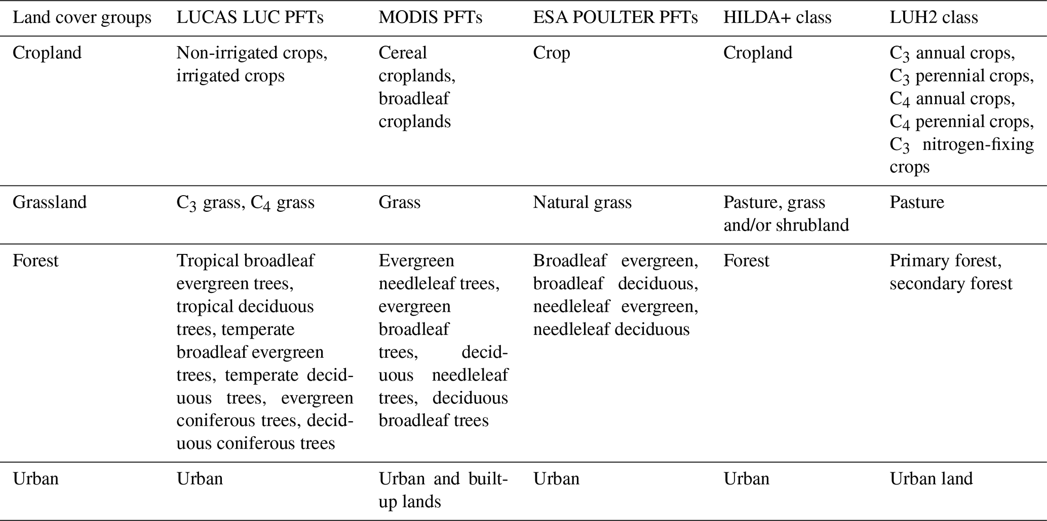
Table 7 Harmonized land cover groups and the corresponding PFTs and land use classes from LUCAS LUC, MODIS, ESA POULTER, HILDA+, and LUH2.

2.5.1 Historical PFT time series based on ESA-CCI LC PFTs

Together with the high-resolution land cover maps, the ESA-CCI provides a dedicated user tool to re-project and re-sample the LULC maps and to translate the LULC classes into model-specific PFTs. During the re-sampling from the native ∼ 300 m horizontal resolution, the LULC class fractions are automatically preserved as fractions per re-sampled grid cell. The user tool provides a generic translation table but also gives the possibility of including user-defined translations. Further, the involvement of climate data within the translation process is possible to a limited extent. In order to prepare the ESA-CCI-based PFT maps for the present comparison, the generic table provided by the ESA is used under consideration of the modifications introduced by Poulter et al. (2015). In addition to adjustments of the LULC class translation, an urban PFT is added (Table A4). The resolution of the aggregated PFT maps can be chosen flexibly as required by the user. For the comparison with the LUCAS LUC PFT maps, the PFT maps, denoted as ESA POULTER in the following, are aggregated to a horizontal resolution of 0.1^∘.

2.5.2 Historical PFT time series based on MODIS

The Collection 6 Terra and Aqua combined MODIS land cover datasets (C6 MCD12Q1) provide ready-to-use PFT maps as one of their 13 science datasets. For C6 MCD12Q1, several processing steps were refined to eliminate known issues from the MODIS Collection 5 datasets, such as the excessively high interannual variability (Abercrombie and Friedl, 2015). Additional information on the MODIS data processing can be found at https://lpdaac.usgs.gov/products/mcd12q1v006/ (last access: 18 August 2023). The annual maps are available globally from 2001 to 2018 at ∼ 500 m horizontal resolution. The 12 MODIS PFTs follow the PFT definition that was developed for the National Center for Atmospheric Research land surface model (NCAR LSM) (Bonan et al., 2002). Table A3 shows the 12 PFTs, including their descriptions. The 13 science datasets provided within C6 MCD12Q1 are available in six different LULC classifications, including the PFT classification. All LULC classifications are generated through employment of a supervised classification algorithm (Sulla-Menashe and Friedl, 2018). For the comparison with the LUCAS LUC dataset, the MODIS PFT maps are aggregated to 0.1^∘ horizontal resolution.

2.5.3 Historical land use and land cover time series based on HILDA+

The HILDA+ (Winkler et al., 2021) dataset provides global land use change information for land use and cover classes (urban, cropland, pasture or rangeland, forest, unmanaged grass or shrubland, sparse or no vegetation) at 1 km resolution from 1950 to 2019. The base map was generated from the Copernicus LC100 dataset (Buchhorn et al., 2020). The land use changes are taken from multiple global (e.g. MODIS MCD12Q1 and ESA-CCI LC) and regional (e.g. CORINE) sources.

3 Results

3.1 Historical LULC

3.1.1 Cropland

Cropland changes in LUCAS LUC correspond well to the changes in LUH2, with some exceptions (Fig. 3a, b). The increase in cropland in Iceland, visible in LUH2, is not present in LUCAS LUC because the LANDMATE PFT, which is used as a base map for LUCAS LUC, has no cropland in Iceland in 2015 (not shown). Moreover, weaker changes in cropland fractions in LUCAS LUC compared to LUH2 are found in the Middle East and in northern Africa. The LUT keeps the fraction of bare ground constant (Sect. 2.3), which limits the magnitudes of possible land cover changes in regions with large bare-ground fractions.

The decrease in cropland fraction in parts of eastern Europe is present in both HILDA+ and ESA POULTER, while the latter shows a smaller magnitude than LUCAS LUC and LUH2, respectively (Fig. 3c, d). The cropland reduction in central and southern Europe in LUCAS LUC is also visible in ESA POULTER. In contrast, HILDA+ shows cropland increases for large regions in Spain, France, and Germany. The strong increase in cropland in southern Russia and north-western Kazakhstan found in ESA POULTER and HILDA+ is not captured by LUCAS LUC and LUH2. In southern Scandinavia and Estonia, the cropland signals in LUCAS LUC, LUH2, and HILDA+ are opposite in comparison to the ESA POULTER-derived signal. For Egypt, ESA POULTER and HILDA+ show a reduction in cropland for the central Nile Delta and along the Nile River and an increase along the edges of the Nile Delta, whereas LUCAS LUC shows only an increase in this region. The increase along the delta edges can be attributed to cropland expansion and the decreases to urbanization (Xu et al., 2017). These small-scale land cover dynamics are not captured by LUH2.

The decreasing trend in cropland is visible in the aggregated values for all the datasets in the three PRUDENCE regions EA, ME, and IP (Fig. 4a–c). Only in MODIS do some years show less cropland compared to the year 2015. LUCAS LUC follows the LUH2 annual area changes closely but with a slightly lower magnitude. MODIS and ESA POULTER show much smaller changes in EA and IP, while ESA POULTER surpasses the LUCAS LUC and LUH2 changes in the period 1992 to 2001 in ME. HILDA+ shows smaller changes in ME than LUCAS LUC. For IP, LUCAS LUC and HILDA+ are very close before 1990 and deviate thereafter. The overall spread of the different LUCAS LUC time series increases with time, originating mainly from the different LUH2 reconstructions. This uncertainty is small compared to the actual changes.

In LUCAS LUC, cropland decreases are even more widespread for most parts of Europe when starting from 1950 (Fig. 6a) instead of 1992 (Fig. 3a). In Mid-Europe especially, a steep decline in cropland cover is visible from the 1950s to the 1970s (Fig. 4b). On the other hand, increases in northern Africa, in Iran, and along the Nile Delta are larger for the longer time period. In addition, the areas with increasing cropland cover in southern Russia and eastern Ukraine expanded compared to the 1992–2015 period. The largest spread in the change signals can be found in parts of Italy, Poland, and Denmark (Fig. 6b). Overall, the fraction of robust changes is 98.9 % for Europe but varies between 95.6 % in the Alps (AL) and 99.9 % in the British Isles (BI) (Table 8).

3.1.2 Irrigated cropland

As described in Sect. 2.3.3, the area development of irrigated cropland follows the trend of LUH2. From 1950 to 2015, the fraction of irrigated cropland increases in most countries in the research area (Fig. 6c). In the western Mediterranean regions, this increase is caused by the decrease in cropland, whereas in the Balkan region, in the Middle East, and in the Transcaucasian region, the relative fraction of irrigated cropland increases. The increase is predominantly evident along freshwater sources such as rivers, channels, lakes, and aquifers. In particular, the increase in irrigated cropland is striking along the Garonne in France, along the Ebro in Spain, along the Euphrates and Tigris in Iraq, and along the Nile in Egypt. Following the results of Thebo et al. (2014), irrigated cropland also appears increasingly around cities (e.g. around Paris in France, Casablanca in Morocco, and Tripoli in Libya). The spread of the climate change signal is large in many parts of the Mediterranean region and the Middle East, with the largest spread in Iraq (Fig. 6d). However, the spread is still smaller than the changes resulting in fractions of robust changes above 95 % for all the regions (Table 8).

3.1.3 Grassland

While LUH2 shows a decrease in grassland (i.e. land use class pasture) in Spain and Poland (Fig. 3f), LUCAS LUC shows an increase in grassland (Fig. 3e). The reduction in grassland in LUH2 is mainly driven by conversion of non-forested vegetation to pasture, which compensates for the increase in pasture converted from cropland. However, in LUCAS LUC the non-forested vegetation that can be converted into grassland is shrubland (Tables 5 and 6), which is sparsely present in Poland and parts of central Spain (not shown). This limits the extent to which the LUT can increase grassland by decreasing shrubs. Consequently, other transitions (e.g. from cropland to pasture) dominate the land cover change signal for grassland. While LUCAS LUC grassland changes do not follow the pasture changes in LUH2, they are closer to the strong pasture increase in Poland found by Kuemmerle et al. (2016), who used data from the Common Agricultural Policy Regionalized Impact (CAPRI) database. Just like the cropland changes, alterations of grassland fractions are weaker in LUCAS LUC compared to the pasture changes in LUH2 in the Middle East (Fig. 3e, f). This can be partly attributed to the larger share of bare ground in this region in LUCAS LUC.

The changes in grassland are quite small in ESA POULTER, except for southern Russia and north-western Kazakhstan, where a dual pattern of decrease and increase can be seen (Fig. 3g). The decrease in grassland in this region results from a conversion into cropland (Fig. 3c), which LUH2 does not capture.

The time series of grassland changes for the three PRUDENCE regions show substantial differences between the datasets (Fig. 4d–f). Since LUH2 does not provide grassland cover, pasture area changes are plotted instead. This is likely the reason why LUCAS LUC changes deviate more strongly from LUH2 when changes in grassland are compared. For IP and EA, the spread of the change signal is small compared to the magnitude of the change signal, while it is a similar size in ME. In contrast to the cropland changes, the spread originates mainly from the difference in the resolution between LUCAS LUC and LUH2.

The grassland cover increases in many of the eastern European countries from 1950 to 2015, with the exception of Estonia, Slovenia, and the Czech Republic (Fig. 6e), which show a decrease in grassland. In addition, Portugal and Türkiye show an increase in grassland. Decreasing grassland cover is found in central and southern Europe as well as in Scotland and parts of Russia. In contrast to the shorter period from 1992 to 2015, the grassland cover increases in northern Germany, northern France, England, and Ireland between 1950 and 2015. The grassland changes show a spread throughout most of southern, central, and eastern Europe (Fig. 6f). This also results in a lower fraction of robust changes in comparison with the other land cover classes (Table 8). For the European domain, the fraction is 94.4 %, but ME, France (FR), and BI only have fractions of 82.5 % to 86.4 %.

3.1.4 Forest

Forest changes in LUCAS LUC match the LUH2 changes closely (Fig. 3h, i). Increases in forest fractions in mountainous areas (e.g. the Alps, Carpathians, Balkans, or Pyrenees), Great Britain, Ireland, and Russia of between 55 and 60^∘ are found in both datasets. The increases in northern Italy and Ireland are weaker in LUCAS LUC compared to LUH2. This is again caused by the difference in forest cover in LUCAS LUC and LUH2 in the year 2015. The LUT can only decrease as much forest fraction backward in time (i.e. increase for the comparison between 1992 and 2015) as is available in 2015. A decreasing forest fraction can be seen in Russia (e.g. east of Belarus and at the border with Georgia) and in Albania. As for cropland and grassland, forest changes in LUH2 and thus also in LUCAS LUC differ in many regions compared to ESA POULTER and HILDA+ (Fig. 3j, k). The change signals tend to be reversed between LUCAS LUC and/or LUH2 and ESA POULTER, with a decrease in mountainous areas (e.g. the Alps, Pyrenees, or Balkans) and an increase near the Russian border with Belarus. The decreases in the Alps and Pyrenees especially seem not to be supported by HILDA+ and recent assessments. For example, Fernández-Nogueira and Corbelle-Rico (2018) found a strong afforestation signal between 1990 and 2012 in the northern parts of Spain based on the CORINE Land Cover dataset. In addition, inventory-based datasets show an increase in forest cover during the 1990s and 2000s for the Alps (e.g. Schwaab et al., 2015; Bebi et al., 2017). Substantial forest fraction increases in northern Russia, northern Norway, and northern Finland can be seen in ESA POULTER and HILDA+. In these regions, both LUCAS LUC and LUH2 show no change in forest fraction at all. In these areas forest cover increased due to forest growth instead of active afforestation (Potapov et al., 2015), which seems to be captured by the satellite-based ESA POULTER dataset but not by LUH2.

Forest cover increases in both LUH2 and LUCAS LUC in the PRUDENCE regions EA, ME, and MD (Fig. 4g–i). In EA, ESA POULTER also shows a increase in forest cover but with a smaller magnitude, while MODIS forest cover shows both increases and decreases. The differences between LUH2 and LUCAS LUC compared to the two satellite-based datasets are more substantial in ME. Here, ESA POULTER shows a strong decrease, while MODIS shows both strong increases and decreases for some years. In the IP region, LUCAS LUC, LUH2, MODIS, and especially HILDA+ show an increase in forest cover, while ESA POULTER shows a decrease. The increases are much more pronounced in the HILDA+ dataset. The afforestation trend in IP is mostly due to farmland abandonment (Vilà-Cabrera et al., 2017; Palmero-Iniesta et al., 2021). While the cropland decrease is also present in LUCAS LUC, cropland is mainly converted into shrubland except for northern Spain (not shown).

The expansion in forest cover in LUCAS LUC is more pronounced for the period 1950 to 2015 (Fig. 6g) than for the period 1992 to 2015 (Fig. 3). Especially in the Alps, Balkans, Caucasus, Scotland, Estonia, and Lithuania, forest cover increases substantially. In addition, for the longer time period forest cover increase is found in Sweden and Finland. An increase in forest cover in Finland was also found by Gao et al. (2014), who related these changes to the conversion of peatland into forest. Areas with forest cover reduction in Russia are smaller in extent and in magnitude compared to the period 1992 to 2015. Interestingly, Iceland experienced a decrease in forest over the longer time period compared to an increase for the shorter time period, which is likely due to the strong government-led reforestation efforts initiated in the 1980s and 1990s (Halldorsson et al., 2008). The spread of the LUCAS LUC reconstructions is noticeable in regions with a strong forest cover increase (Fig. 6h). For Europe, 95.4 % of changes are widely robust; only BI and EA have a lower fraction of robust changes. In addition, the extent of slight increases is uncertain, while larger changes in this region are more robust (not shown).

3.1.5 Urban

Changes in urban areas are limited to the major urban agglomerations in LUCAS LUC and LUH2 (Fig. 3l, m), while ESA POULTER (Fig. 3n) also shows a more widespread urbanization in rural areas in central and eastern Europe. HILDA+ shows widespread increases but also decreases in some parts of central and eastern Europe (Fig. 3o). Aggregated for the EA, ME, and IP regions, all the datasets show an urbanization signal (Fig. 4j–l). LUCAS LUC and HILDA+ show a larger trend in the European urbanization signal before 1990 that was also found in other studies (e.g. Güneralp et al., 2020; Tian et al., 2022). In contrast, the rapid urbanization in the ESA POULTER dataset in the early 2000s seems to be too strong. Reinhart et al. (2021) showed that the urban area fraction in ESA-CCI LC increased by 60 % between 2000 and 2006 in eastern European countries compared to 6 % in CORINE. Overall the different land cover datasets show large differences in the urbanization trend, with LUH2 and, therefore, LUCAS LUC at the moderate end and HILDA+ at the upper end.

The urban fraction of LUCAS LUC increase for the period 1950 to 2015 (Fig. 6i) is larger and more widespread compared to the signal from 1992 to 2015 (Fig. 3l). A strong urbanization signal is visible for Madrid, Paris, and Moscow. A larger-scale increase is found in England, northern Italy, the Benelux region, western Germany, Poland, and Slovenia. The urbanization signal is hardly affected by the uncertainties due to the LUH2 reconstructions but shows smaller changes in the 0.1^∘ dataset compared to the 0.25^∘ dataset, which is closer to the LUH2 changes (Fig. 4j–l). Despite these differences, the spread is smaller than the actual changes, which leads to a high number of robust changes in all the regions (Table 8).

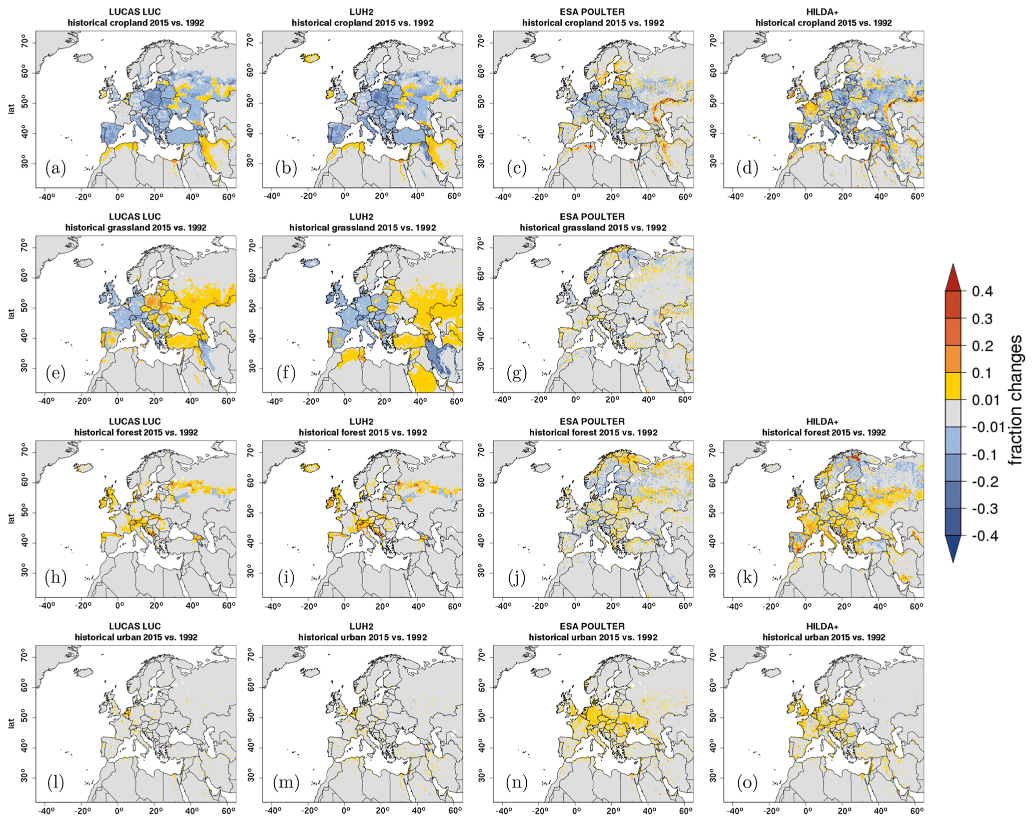
Figure 3 Changes in grid cell fractions for the cropland (a–d), grassland (e–g), forest (h–k), and urban (l–o) classes based on LUCAS LUC (a, e, h, l), LUH2 (b, f, i, m), ESA POULTER (c, g, j, n), and HILDA+ (d, k, o) between 1992 and 2015. For LUCAS LUC, only those changes are shown where all LUCAS LUC reconstructions agree on the sign of the change (Sect. 2.4). Please note that for LUH2 pasture is taken as the grassland class and HILDA+ does not provide a grassland class.

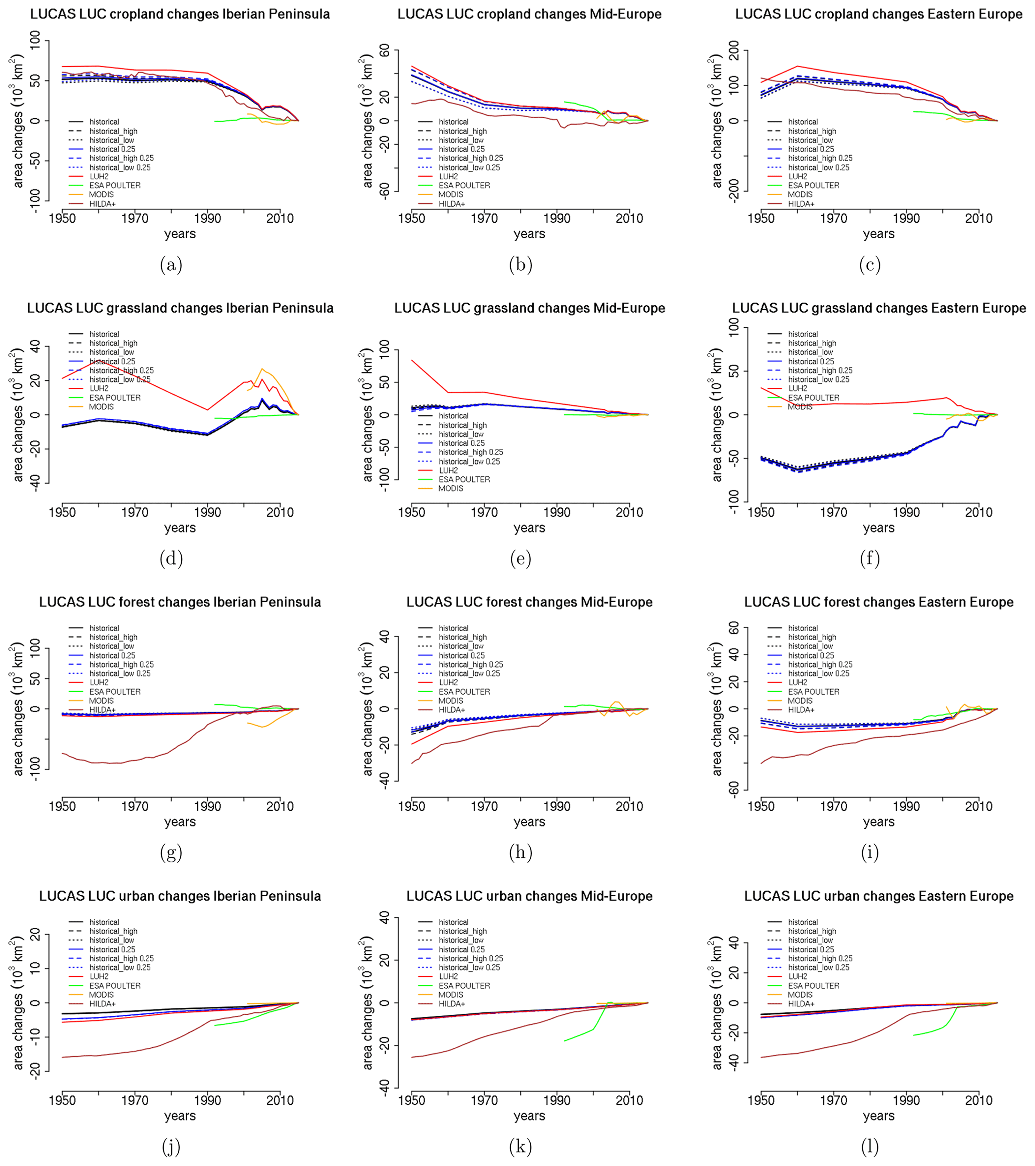
Figure 4 Area changes with respect to the year 2015 in cropland (a–c), grassland (d–f), forest (g–i), and urban (j–l) computed for LUCAS LUC, LUH2, ESA POULTER, MODIS, and HILDA+ for the PRUDENCE regions Iberian Peninsula (a, d, g, j), Mid-Europe (b, e, h, k), and Eastern Europe (c, f, i, l). In addition, values for LUCAS LUC at different resolutions and based on different LUH2 reconstructions are provided. Please note that for LUH2 pasture is taken as the grassland class.

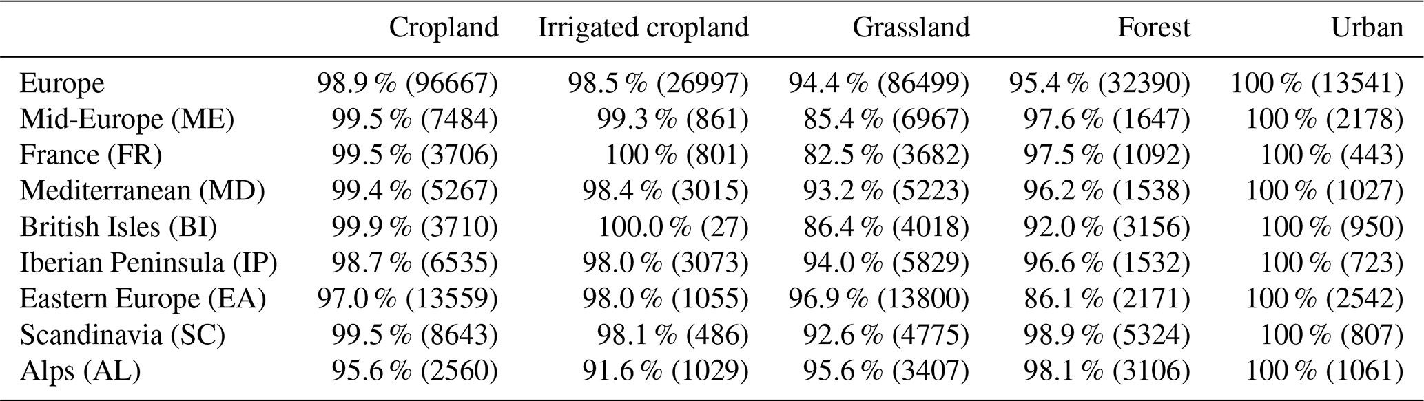
Table 8 Percentage of robust changes (Sect. 2.4) with an absolute value >0.01 for the different land cover types for Europe (30–70^∘ N, 25^∘ W–50^∘ E) and the PRUDENCE regions. The total number of grid cells with changes > 0.01 is given in parentheses.

3.1.6 Forest type

In Fig. 5, the annually averaged broadleaf / needleleaf forest ratio of the LUCAS LUC dataset with and without McGrath data (Sect. 2.3), the original McGrath dataset, ESA POULTER, and MODIS for different PRUDENCE regions is presented. Without employing the McGrath dataset, the broadleaf / needleleaf ratio is almost constant throughout the historical period because the relative fractions within a PFT group are preserved during the LUT transition computation. As intended, the trends in LUCAS LUC with McGrath employed are close to the trends in the original McGrath dataset, while the absolute values differ. The two satellite-based datasets, ESA POULTER and MODIS, do not show strong trends in the broadleaf / needleleaf ratio until 2010 (the last year of the McGrath dataset). For eastern Europe, the trends are the opposite, with a slight increase in the broadleaf / needleleaf ratio in ESA POULTER and MODIS and a larger decrease in McGrath and LUCAS LUC.

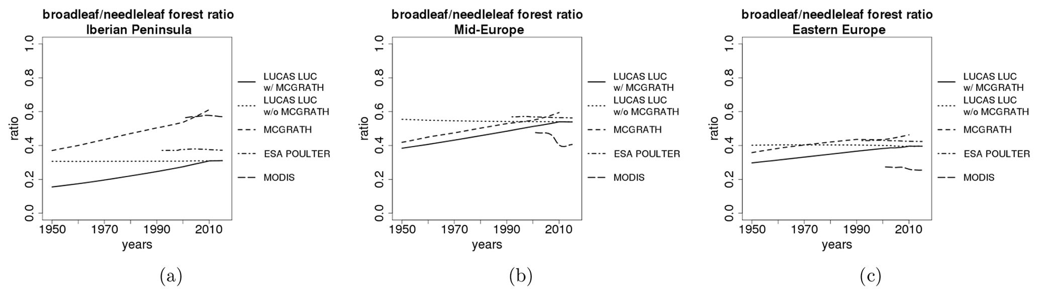
Figure 5 Ratios of broadleaf and needleleaf PFTs computed for LUCAS LUC with and without McGrath forest type data, ESA POULTER, and MODIS for the PRUDENCE regions (a) Iberian Peninsula, (b) Mid-Europe, and (c) Eastern Europe.

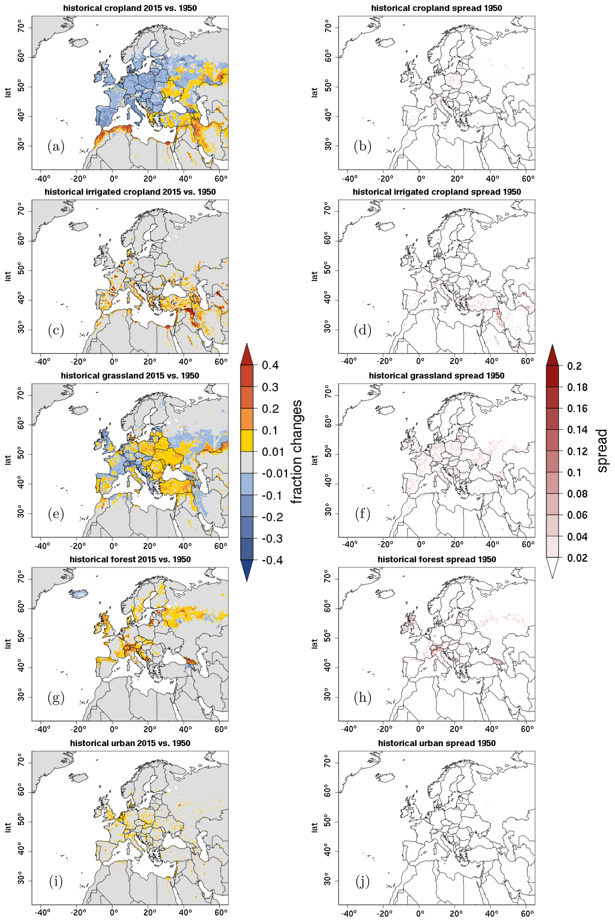
Figure 6 Changes in grid cell fractions and the spread of the changes (Sect. 2.4) for the (a, b) cropland, (c, d) irrigated cropland, (e, f) grassland, (g, h) forest, and (i, j) urban classes based on LUCAS LUC between 1950 and 2015. Only those changes are shown where all LUCAS LUC reconstructions agree on the sign of the change (Sect. 2.4).

3.2 Future LULC

Future changes in land cover fractions between 2015 and 2100 for the eight different scenarios (Table A2) are presented in Figs. 7–11. Aggregated area changes for the three PRUDENCE regions IP, ME, and EA as well as for Europe (30–70^∘ N, 25^∘ W–50^∘ E) are shown in Figs. 12–15.

3.2.1 Cropland

While cropland fractions decrease in the historical period from 1950 to 2015 over most of Europe (Fig. 6a), a continent-wide decrease until 2100 is projected only for the SSP3–RCP7.0 scenario (Fig. 7h), with the exception of France, Türkiye, and Belarus. The two SSP1-based scenarios show very similar patterns of cropland changes, with strong expansion in western Russia and large decreases in southern Russia, Ukraine, Hungary, England, Denmark, and northern Germany. The strongest increase in cropland is found for the SSP4–RCP3.4 scenario. The SSP5–RCP8.5 scenario shows small changes over Europe and large cropland decreases in northern Africa and the Middle East. Large block-like features are visible in Scandinavia, Russia, and Türkiye for most of the scenarios, which have an extent of about 2^∘ and are likely caused by the LUH2 workflow (Sect. 4.2).

The temporal evolution of aggregated cropland area shows that the changes are not steady for all the scenarios (Fig. 12). For instance, the cropland area for Europe and in particular for the ME region shows a rapid increase from 2050 onwards in SSP5–RCP3.4OS while staying rather constant before (Fig. 12a, c). The two SSP1 scenarios diverge in their evolution around 2025 for Europe and the IP and ME regions but rather converge at the end of the century (Fig. 12a–c). While showing a slight decrease in cropland cover aggregated for Europe, the cropland area stays almost constant in the three PRUDENCE regions for SSP5–RCP8.5.

3.2.2 Irrigated cropland

For the future scenarios, the irrigated cropland fractions show different signals depending on the region (Fig. 8). Signals for SSP1–RCP1.9, SSP1–RCP2.6, and SSP3–RCP7.0 (Fig. 8a, b, g) go in the same direction (increase) but with different magnitudes. While the SSP1-based scenarios show small changes, the SSP3–RCP7.0 scenario projects large changes predominantly in the Middle East (Urmia basin) and Türkiye, where a strong increase in irrigated cropland is expected.

The strongest changes for Europe are projected by the SSP5–RCP3.4OS scenario, which shows a continent-wide increase in irrigated cropland (Fig. 8d) and cropland in general (Fig. 7d). Exceptions such as regions along the Po River in Italy and along the Euphrates and Tigris in Iraq show a decrease in irrigated cropland for this scenario.

In contrast to the continent-wide increase in irrigated cropland in the SSP5–RCP3.4OS scenario, the SSP4-based scenarios with the RCP3.4 (Fig. 8c) and RCP6.0 (Fig. 8f) pathways project a continent-wide decrease in irrigated cropland, with some exceptions around the Mediterranean Sea, along Africa's western coast, and in central Asia.

Most scenarios agree on the change signal in multiple regions. While regions along the Euphrates and Tigris in Iraq, along the Nile in Egypt, and along the Po River in Italy expect a decrease in irrigated cropland in most scenarios, regions in the North Caucasus and in the Urmia basin in Iran show an increase in irrigated cropland in most scenarios.

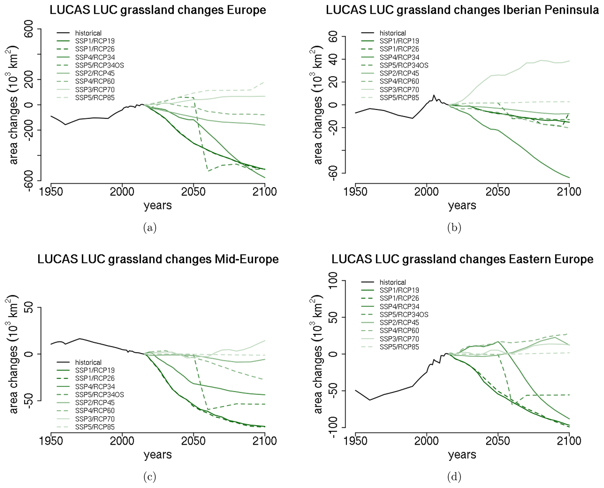
3.2.3 Grassland

The SSP1-based scenarios together with SSP4–RCP3.4 and SSP5–RCP3.4OS (Fig. 9a–d) show a strong decrease in grassland cover for most of Europe. For SSP1–RCP1.9 and SSP1–RCP2.6, this is due to the conversion of grassland to forest (Fig. 10a, b), while for SSP4–RCP3.4 and SSP5–RCP3.4OS grassland is mainly converted to cropland (Fig. 9c, d). Similarly, the increase in grassland in southern Russia in the SSP4–RCP3.4 scenario is due to the conversion from cropland to grassland. The grassland decrease is not as strong in the SSP2–RCP4.5 and SSP4–RCP6.0 scenarios, where large regions with increases are also visible (Fig. 9e, f). The SSP3–RCP7.0 scenario shows a number of regions with a large grassland cover increase, such as Spain, Germany, Norway, the Alps, and the Carpathians (Fig. 9g). The increase in Norway and in the Alps is compensated for by deforestation (Fig. 10g). Almost no changes in grassland cover over Europe are visible for the SSP5–RCP8.5 scenario (Fig. 9h). However, a large increase is found in northern Africa and the Middle East, which is compensated for by a decrease in cropland (Fig. 7h). The block-like structures that are found for the cropland changes are also visible for the grassland changes.

Except for SSP5–RCP3.4OS, which shows a strong abrupt decrease from 2050 to 2055, increase and decrease in grassland cover over Europe are steady from 2015 onwards (Fig. 13a). The abrupt change in SSP5–RCP3.4OS is even more pronounced in the ME and EA regions (Fig. 13c, d). In the latter region, the SSP4–RCP3.4 scenario also shows a steep decline in grassland cover after 2050. While grassland cover strongly increases in one scenario (Fig. 13b) in the IP region, grassland cover either stays almost constant over time or decreases in the other two regions.

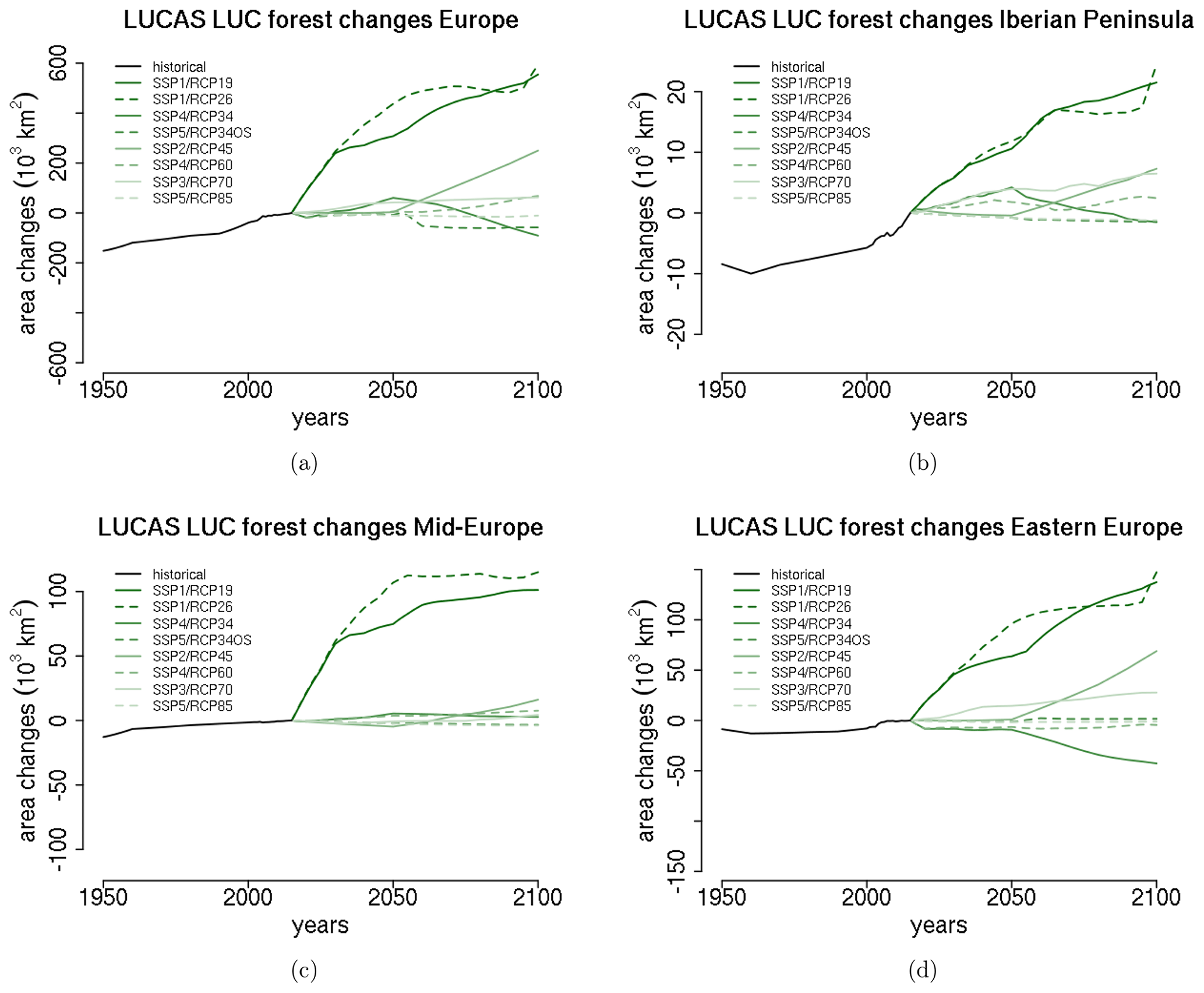
3.2.4 Forest

A strong forest cover increase is found for SSP1–RCP1.9, SSP1–RCP2.6 (Fig. 10a, b), and, to a lesser extent, SSP2–RCP4.5 (Fig. 10e). These are the scenarios for which the added tree cover fraction files are used because the original LUH2 dataset underestimates the strong afforestation signal (Sect. 2.3.2). In the SSP1-based scenarios, the largest increase is found in Ireland, in England, in northern France, and in Russia near the border with Ukraine. Also, a widespread increase is visible for most countries in central and eastern Europe, southern Sweden and Finland, and northern Spain. The forest increase is mainly compensated for by a decrease in grassland (Fig. 9) and shrubland (not shown) and to a lesser extent by declining cropland (Fig. 7). The only region with substantial forest reduction is western Russia. This decrease is also visible in the SSP4–RCP3.4, SSP5–RCP3.4OS, and SSP2–RCP4.5 scenarios (Fig. 10c–e). As for cropland and grassland, SSP5–RCP8.5 shows only small forest cover changes (Fig. 10h).

The aggregated forest cover changes for Europe show a steep increase from 2016 onwards (Fig. 14a). In the ME region, the forest cover increase levels off around 2050, while the IP and EA regions show steady increases (Fig. 14b–d). Especially in the ME and EA regions, the magnitude of the increase is many times larger than for the changes in the historical period. In contrast, the afforestation in the SSP2–RCP4.5 scenario starts in 2050 and continues until 2100, with a magnitude comparable to historical changes. A substantial deforestation signal in SSP2–RCP4.5 is visible in the IP and EA regions from 2050 onwards.

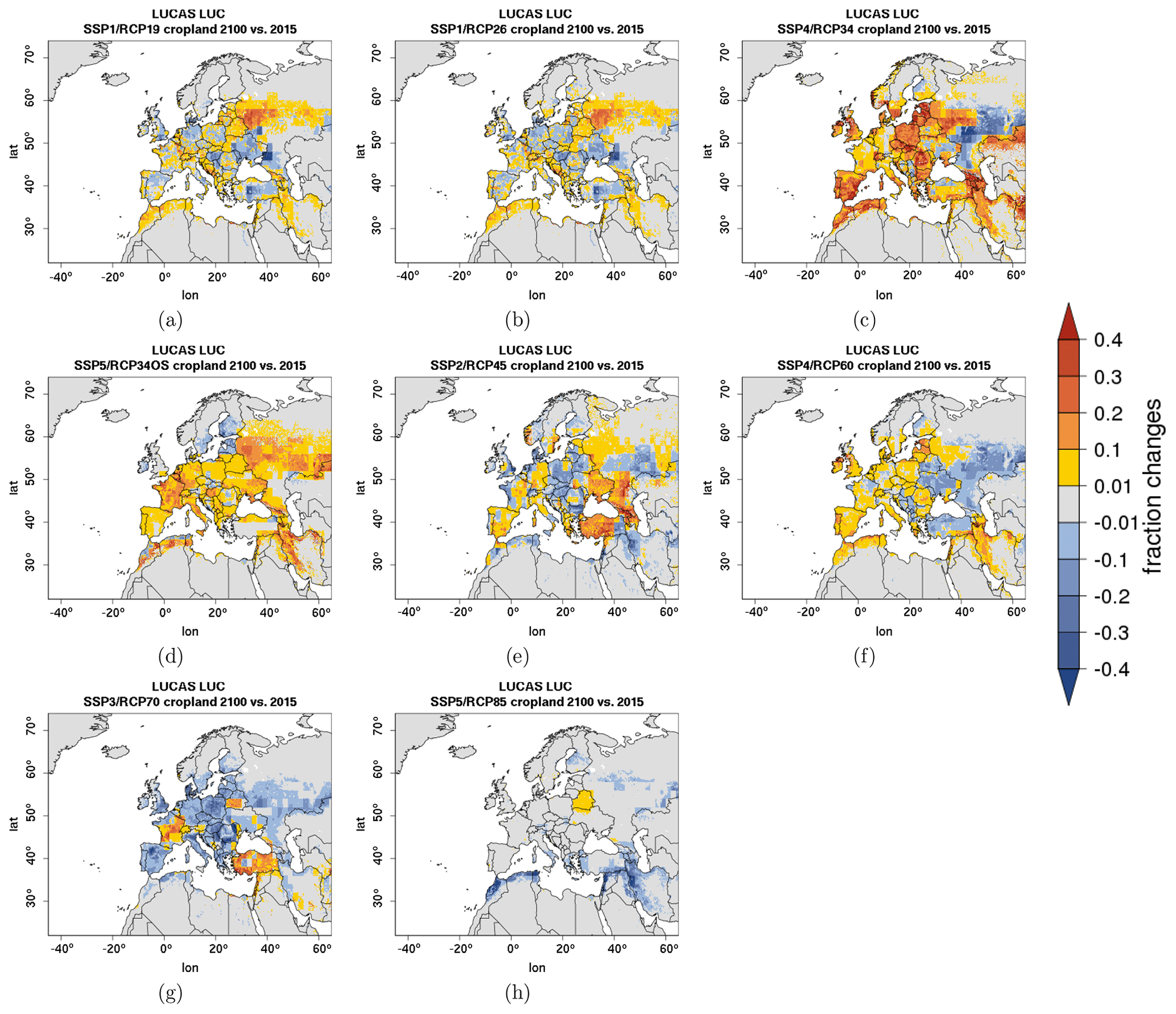
Figure 7 Changes in grid cell cropland fractions based on LUCAS LUC for the RCP–SSP scenarios (a) SSP1–RCP1.9, (b) SSP1–RCP2.6, (c) SSP4–RCP3.4, (d) SSP5–RCP3.4OS, (e) SSP2–RCP4.5, (f) SSP4–RCP6.0, (g) SSP3–RCP7.0, and (h) SSP5–RCP8.5 between 2015 and 2100.

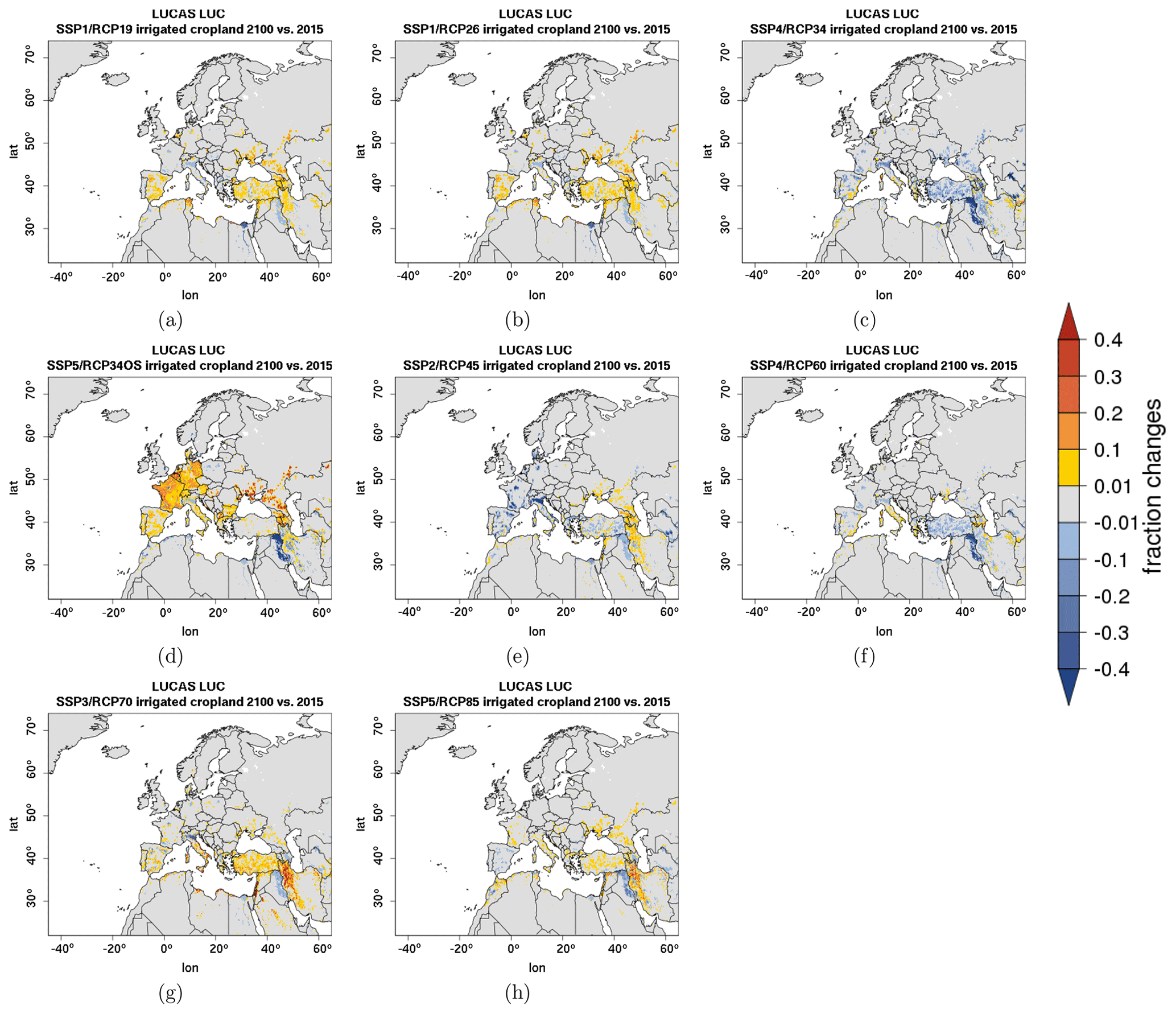
Figure 8 Same as Fig. 7 but for irrigated cropland PFTs.

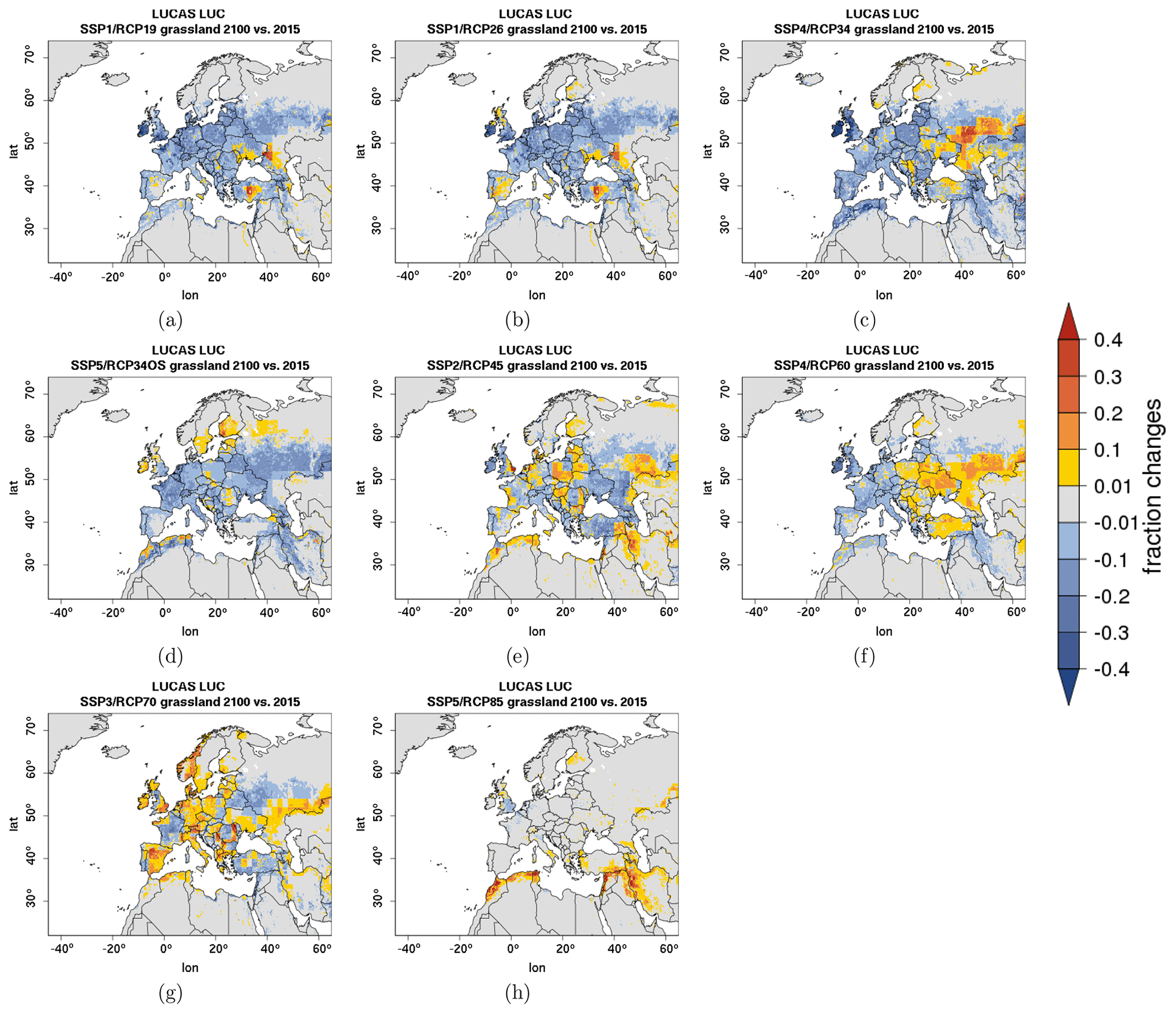
Figure 9 Same as Fig. 7 but for grassland PFTs.

Figure 10 Same as Fig. 7 but for tree PFTs.

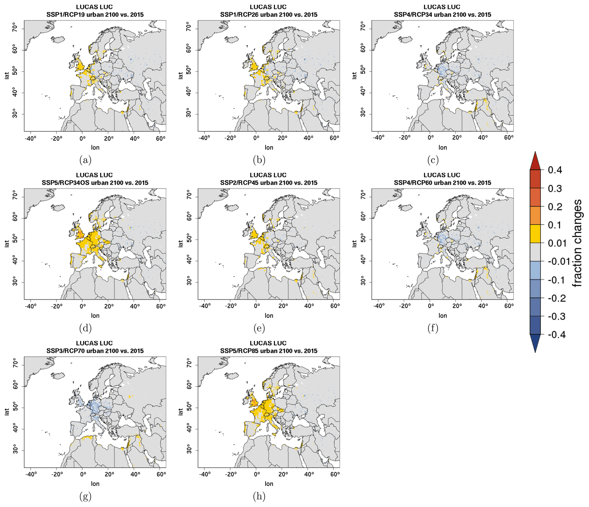
Figure 11 Same as Fig. 7 but for urban.

3.2.5 Urban

In contrast to the historical period, all the scenarios show both decreases and increases in urban fraction between 2015 and 2100 (Fig. 10). Urban changes are largely driven by the SSP scenarios (i.e. population dynamics), resulting in almost identical changes in the LUCAS LUC dataset in scenarios based on the same SSP scenario. A widespread urbanization signal can be found in the SSP5-based scenarios for Europe except for eastern Europe, which shows a decrease in urban fraction (Fig. 10d, h). The increase in urban fractions is particularly strong in Great Britain. The SSP1-based scenarios show an increase with a smaller magnitude in western and southern Europe and Scandinavia, respectively, and a decrease in the eastern European countries, including some parts of Germany (Fig. 11a, b). Based on the SSP4–RCP6.0 scenario, only a few urban areas in Spain, France, Italy, England, and the Czech Republic exhibit an increase in urban fraction. In eastern and central Europe urban fraction decreases, with Germany experiencing the largest decrease. The SSP3–RCP7.0 scenario is the only scenario that does not show a decrease in urban fraction in Russia. Instead, it shows decreases in western and central European countries.

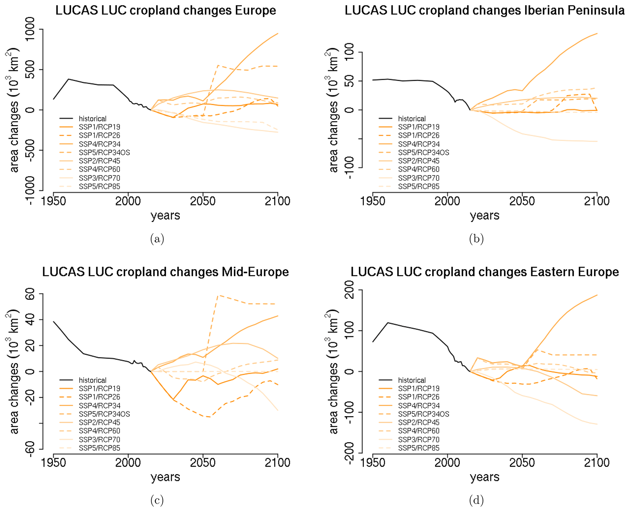
Figure 12 Area changes with respect to the year 2015 in cropland PFTs computed for LUCAS LUC for (a) Europe and the PRUDENCE regions (b) Iberian Peninsula, (c) Mid-Europe, and (d) Eastern Europe.

Figure 13 Same as Fig. 12 but for grassland PFTs.

Figure 14 Same as Fig. 12 but for tree PFTs.

Figure 15 Same as Fig. 12 but for urban.

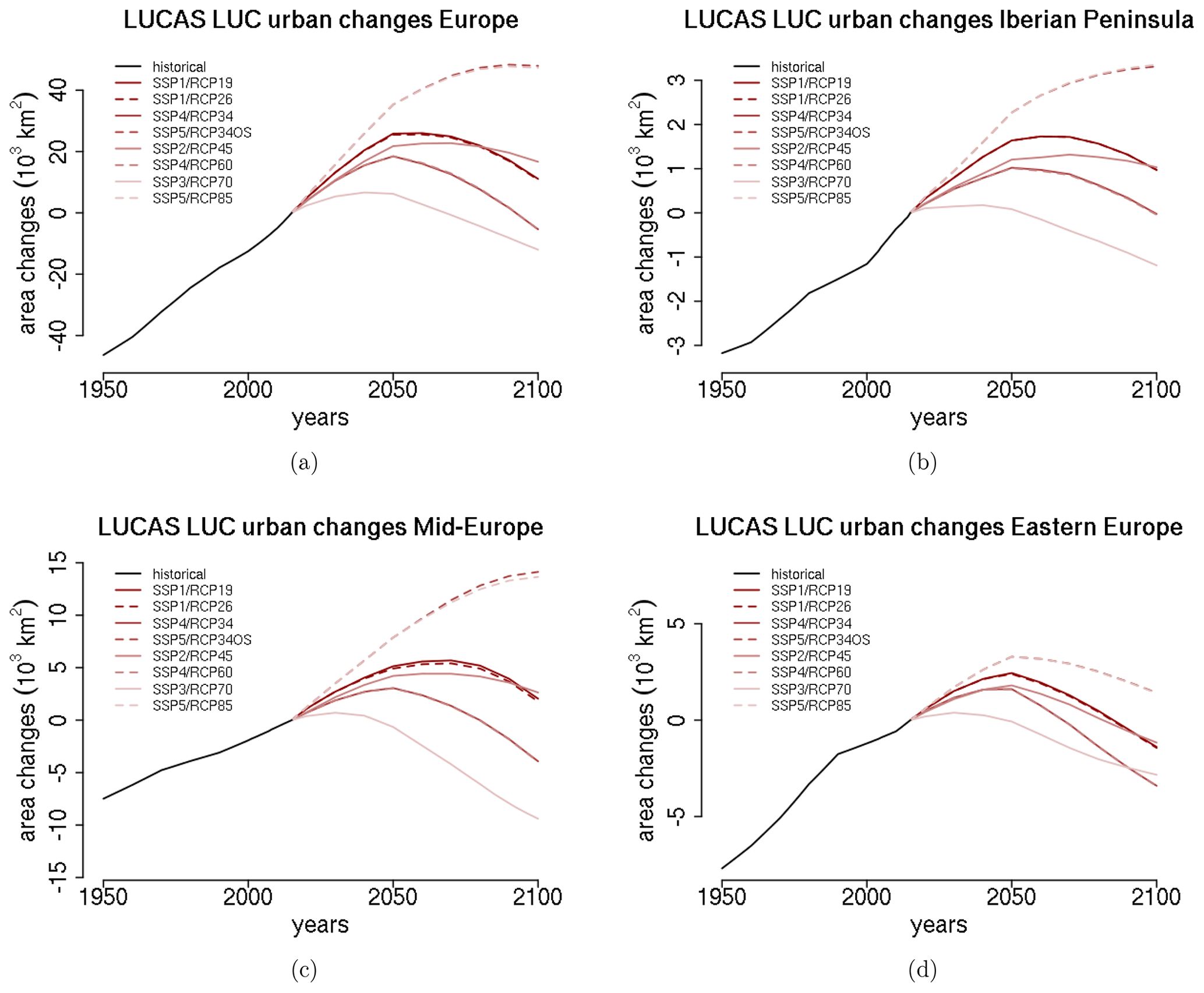
The time series analysis of the aggregated changes for Europe shows that all the scenarios project an increase in urbanization until 2050 (Fig. 15a). Only in the SSP5-based scenarios does the total urban area increase further until 2100. For the other scenarios, urban fraction remains constant or declines. However, there are regional differences. In the EA region, all the scenarios show a peak in urbanization until 2050 and a decrease until 2100, with the exception of SSP3–RCP7.0, where the peak is already reached by 2040 (Fig. 15d). The IP and ME regions show a similar temporal evolution of urban areas (Fig. 15b, c). However, the decrease is stronger in ME. Here, the total urban area in 2100 is even smaller than the total area in 1950 in the SSP3–RCP7.0 scenario.

4 Discussion

4.1 Uncertainties

The uncertainties in the LUCAS LUC dataset with respect to the historical changes were subdivided into the uncertainty in the underlying base map for 2015 (i.e. the LANDMATE PFT map), the uncertainties in the LUH2 datasets, and the different resolution between the LANDMATE PFT map (0.1^∘) and the LUH2 dataset (0.25^∘).

The uncertainty in the present-day pattern of the land cover (i.e. the LANDMATE PFT map) was assessed for Europe in the companion paper (Reinhart et al., 2022b). The ESA-CCI LC dataset, which is the baseline for the LANDMATE PFTs, was previously validated globally (e.g. Hua et al., 2018) and in a regional approach limited to eastern Europe (e.g. Reinhart et al., 2021). Depending on the validation method, which is a limiting factor in such a validation assessment, the ESA-CCI LC dataset was shown to be of a very good quality for the dominant land cover classes cropland and forest, but certain issues were found for the other classes. Reinhart et al. (2021) showed an overall accuracy of 76 % for the ESA-CCI LC dataset in eastern Europe, where cropland and forest showed > 81 % accuracy but accuracy values lower than 50 % for the other categories assessed. Some shortcomings of ESA-CCI LC could be overcome through targeted variation of the LANDMATE PFT cross-walking procedure (CWP). For example, the known too small shrub proportions of ESA-CCI LC over Europe were partly compensated for by increasing the shrub proportions for certain land cover class translations into PFTs.

Therefore, compared to ESA POULTER, the map generated using the CWT by Poulter et al. (2015), the LANDMATE PFTs were improved for shrubland, forest, grassland, and bare-area cover, respectively, and were slightly worse for cropland, which is discussed in the associated publication by Reinhart et al. (2022b). The overall accuracy of the LANDMATE PFT dataset is about 73 %.

The uncertainties from the LUH2 dataset are discussed by Hurtt et al. (2020), and the additional uncertainty information, in the form of two different historical reconstructions, was employed in the present study to quantify the impact of this uncertainty on the historical changes within LUCAS LUC. The results of this analysis show that this uncertainty increases with time and that the different LUH2 reconstructions have the largest contribution to the spread of the changes except for urban land cover, where the resolution differences are more important. Overall, the majority of the changes between 1950 and 2015 are larger than the spread, with fractions of robust changes of 90 % and higher for most land cover classes and regions in Europe. Only grassland and forest changes are lower for some regions, with the lowest values for grassland changes in FR (82.5 %).

The differences in historical LULCC between the LUCAS LUC and other LULCC datasets are mainly caused by the differences between LUH2 and the other datasets due to the close connection between LUCAS LUC and LUH2 LULCC. Li et al. (2018), who compared ESA-CCI LC with LUH2 and other available global datasets, attributed these differences (1) to the treatment of shifting cultivation, (2) to the still coarse resolution of ESA-CCI LC (which limits the detection of land cover changes to larger-scale changes), and (3) to the difference between the inventory-based approach (i.e. countries report the land use statistics to the FAO) taken by LUH2 and the satellite-based approach taken by ESA-CCI LC. For instance, Keenan et al. (2015) noted that cleared forest due to wood harvesting is not reported as forest loss if secondary forest is planted because the land use does not change.

Differences between LUCAS LUC and the two datasets ESA POULTER and HILDA+ are most pronounced with respect to forest changes. Kuemmerle et al. (2016) noted that satellite-based datasets include naturally driven changes due e.g. to forest fire and wind storms as well as management-driven changes due e.g. to wood harvesting. Ceccherini et al. (2020) showed that, averaged over Europe, such changes are small compared to forest harvesting but can be larger in regions with frequent forest fires (e.g. Portugal). Also, the different definition of forest in LUH2, which is based on a biomass density threshold, and ESA-CCI LC, which is based on tree cover, could have a substantial impact on the forest transitions. For instance, the afforestation signal over the Iberian Peninsula is mainly due to farmland abandonment and the regrowth of natural vegetation (Vilà-Cabrera et al., 2017; Palmero-Iniesta et al., 2021). A detailed analysis of the ESA POULTER time series is needed to investigate whether these processes caused the discrepancies in forest changes between LUH2 and LUCAS LUC on the one hand and HILDA+ and ESA-CCI LC on the other hand. Another possibility is the already mentioned uncertainty originating from the CWP. However, the impact of the CWP on the computed land cover changes has not been analysed so far.

Notable differences between LUCAS LUC and ESA POULTER or HILDA+ are also found in the urban land cover changes. Here, ESA-CCI LC seems to largely overestimate the rate of urbanization in Europe between the late 1990s and the early 2000s, whereas urban land cover changes in LUCAS LUC seem to be more reasonable during this period. The other satellite-based PFT time series generated from MODIS shows much larger annual land cover changes that for some regions seem questionable. On the other hand, urban cover changes in MODIS are likely too small. Güneralp et al. (2020) showed that, based on a literature review, the average increase in urban land cover ranges between 2 % yr⁻¹ and 3 % yr⁻¹ in Europe in the 1990s and the 2000s. The large urban changes in HILDA+ could be caused by the difference in the definition of urban and therefore lead to different extents of the urban areas. For instance, the HILDA+ urban land cover in ME in 2015 (approximately 90×10³ km²) is more than twice as large as MODIS, ESA POULTER, and LUCAS LUC (approximately 40×10³ km²). Reinhart et al. (2021) and Demuzere et al. (2019) showed that ESA-CCI LC underestimates urban land cover compared to the CORINE and local climate zone (LCZ) maps, respectively, because it misses low-rise built-up areas.

Given the uncertainties and issues with respect to the other LULCC datasets and based on the detailed analysis of the historical land cover changes in the Results section, LUCAS LUC land cover changes are reasonable for the historical period.

4.2 Indented use and limitations

The newly generated LULCC dataset LUCAS LUC is tailored to the requirements of future CMIP6 downscaling experiments within the FPS LUCAS and EURO-CORDEX. The need for high-resolution land cover input is met by employing the ESA-CCI LC dataset, which has a ∼ 300 m grid globally, as a base map for the year 2015. Since most of the state-of-the-art LSMs employ a PFT land cover classification, the ESA-CCI LC was converted into PFTs. This step also helps deal with mixed ESA-CCI LC land cover classes, which can be conveniently converted into classes with similar properties.

As intended, LUCAS LUC land cover changes closely follow the transitions for cropland, urban, and forest provided by LUH2, with some exceptions discussed in the previous section. Hence, by employing the LUCAS LUC dataset, the land use and land cover forcing of the RCMs is consistent with the forcing of the driving CMIP6 GCM data. However, some GCMs do not use all the land use transitions, leaving the transitions of natural vegetation to their dynamic vegetation models. LUCAS LUC changes are generally slightly smaller for all three land cover types in comparison to the LUH2 changes but follow the temporal evolution of LUH2. This can be attributed to the LUT, which keeps the bare-ground fraction constant in LUCAS LUC and limits the possible land cover changes. This was done because LUH2 does not provide information on changes in bare areas. Thus, desertification, urban expansion, and cropland expansion into desert areas are not included in LUCAS LUC. For Europe, those land cover conversions are not common. However, for regions with large desert areas (e.g. northern Africa and the Middle East), this limitation could substantially underestimate land cover changes. In addition, the difference between LUH2 and LUCAS LUC can be partially attributed to the computation of the land cover area from the PFT fractions. For LUCAS LUC, the ESA-CCI LC land–sea mask was used, which also includes rivers and lakes, while this is not the case for the LUH2 land–sea mask. Consequently, it is likely that smaller total area changes are computed in LUCAS LUC compared to LUH2 in regions with lakes and rivers as well as near coastlines.

The main LUCAS LUC land cover change signals for Europe between 1950 and 2015 are the reduction in cropland but with an extension of irrigated cropland, afforestation in mountainous areas, and urbanization. The magnitude and spatial extent of these changes are considerable and are therefore likely to affect the simulated European climate. Even the smaller land cover changes within the ESA-CCI LC dataset altered the climate change signal simulated with an RCM for the period 1992 to 2015 (Huang et al., 2020). However, as discussed before, LUCAS LUC deviates from other available LULCC datasets for some regions and some land cover classes, while the LULCC datasets considerably deviate from each other too. This needs to be considered when analysing and evaluating the downscaled model results for particular regions and the historical period. To assess the sensitivity of the RCM results to the LULCC input, additional ensemble experiments could be set up by employing different historical LULCC datasets.

In addition to the other LULCC datasets, LUCAS LUC also provides historical changes in the broadleaf / needleleaf forest ratio. The conversions of broadleaf forests to needleleaf forests in Europe are not observed by ESA POULTER or MODIS, which might be due to the differences in satellite-based and inventory-based datasets. This discrepancy should be investigated in the future. The irrigated cropland increase in LUCAS LUC is also substantial and is likely to be relevant when investigating historical changes in the climate of southern Europe, where the largest increase occurs. However, the LUCAS LUC dataset does not distinguish between irrigation methods (e.g. sprinkler irrigation or channel irrigation), which might show different effects on the climate (Valmassoi et al., 2020). Hence, there is a need for a high-resolution European-wide dataset with information on the distribution and development of irrigation methods. While a number of RCMs include a parameterization for irrigation, other management practices are more rarely implemented (e.g. fertilizer), and associated processes are often not covered in current RCMs. In the future, it will be important to consider extending the LUCAS LUC dataset in order to cover more aspects of cropland and forest management.

Future land cover changes are even larger than the historical changes for some of the available scenarios. Hence, substantial policy changes would be necessary to reach the number of land cover conversions in the densely populated Europe, where land ownership is both public and private. In addition, there are large regional differences. The two SSP1-based scenarios, which are the low-end scenarios, show a strong afforestation signal compensated for by a decrease in grassland and shrubland. Also, noticeable changes in cropland (both increase and decrease) are projected for these scenarios. Hence, the LULCC-induced climate change signal might be comparable to the greenhouse-gas-induced signal in regions with large LULCC for some seasons (Hirsch et al., 2018). For instance, Davin et al. (2020) showed for an extreme afforestation scenario that temperature changes simulated with RCMs can range up to ±2 K in Europe in the summer season. This emphasizes the need to include LULCC when downscaling GCM or ESM projections based on these scenarios. Interestingly, the high-end SSP5–RCP8.5 scenario shows the smallest land cover changes except for urbanization, where it has the largest signal together with the other SSP5-based scenario (i.e. SSP5–RCP3.4OS). Therefore, it might be harder to detect LULCC-induced regional climate changes given the strong greenhouse gas forcing. In contrast, the SSP3–RCP7.0 scenario, which also has a large greenhouse gas forcing, shows large-scale cropland decreases and regions with deforestation (e.g. the Alps and Scandinavia) as well as afforestation (e.g. the Po Valley and the Carpathians).

It needs to be noted that the future land cover changes provided by LUCAS LUC consider anthropogenic land use changes but do not account for potential latitudinal and altitudinal shifts of the natural vegetation or especially forest due to climate change (McDowell et al., 2020) because the underlying LUH2 data only provide land use changes due to anthropogenic activities. Therefore, the potential northwards expansion of forest in Europe, which is projected under different climate change scenarios (Dyderski et al., 2018), is not included in LUCAS LUC. Furthermore, in contrast to the historical LUCAS LUC reconstruction, the future forest composition does not change, because the relative fractions of the tree and shrub PFTs stay constant during the forward translation. However, both the shift in the composition and the spatial distribution depend on the projected climate by the different ESMs and GCMs and are therefore uncertain.

The large block-like features appearing in the cropland and grassland change signals in all the scenarios might be attributed to the harmonization process within the LUH2 workflow. Annual changes in cropland, grazing land, and urban areas are computed and aggregated to a 2^∘ grid and subsequently disaggregated to the final 0.25^∘ grid (Hurtt et al., 2020). It is therefore likely that the disaggregation step did not fully dissolve the grid structure of the coarse 2^∘ grid. For GCMs or ESMs with a typical resolution of around 1^∘ this might not have caused any issues. However, for RCMs with a typical resolution of about 0.1^∘, for which the LUCAS LUC dataset has been created, the impact of such structures on the LULCC needs to be carefully investigated.

5 Data availability

The LUCAS LUC historical land use and land cover change dataset (version 1.1) and the LUCAS LUC future land use and land cover change dataset (version 1.1) are published with the Long Term Archiving Service (LTA) for large research datasets which are relevant for climate or Earth system research of the German Climate Computing Service (DKRZ). The DKRZ LTA is accredited as a regular member of the World Data System. Both datasets are available within the LANDMATE project data at https://doi.org/10.26050/WDCC/LUC_hist_EU_v1.1 (Hoffmann et al., 2022b) and https://doi.org/10.26050/WDCC/LUC_future_EU_v1.1 (Hoffmann et al., 2022a). Within the LANDMATE project, a short document summarizes the technical information on the LANDMATE PFT and the LUCAS LUC dataset.

6 Conclusions

The need of the RCM community for a high-resolution LULCC dataset is met using high-resolution PFT maps based on the ESA-CCI LC dataset and land use change information from the LUH2 dataset that was translated into PFT changes using a newly developed LUT. The resulting LUCAS LUC dataset is tailored to RCM requirements. Urbanization, which is mostly discarded by LUTs, is included as well as changes in irrigated cropland. For the historical period, changes in the broadleaf / needleleaf forest ratio are also considered, employing an additional forest type dataset by McGrath et al. (2015).

The LUCAS LUC dataset enables RCM modellers to include historical and future annual LULCC in the next-generation downscaling experiments (e.g. within FPS LUCAS and EURO-CORDEX) based on CMIP6 projections. Consequently, the impact of LULCC on the regional climate change signals can be investigated. For most of Europe, past and future trends in cropland, forest, and urban areas in LUCAS LUC are consistent with the LUH2 dataset, albeit with a slight underestimation of the magnitude. A comparison with other global datasets revealed substantial differences in the trend of some land cover classes. However, the differences between the ESA-CCI LC-based dataset and the MODIS-based dataset are also quite large, showing the uncertainty related to the approaches employed to estimate LULCC.

The future LULCC for the eight SSP–RCP scenarios shows substantial changes that can exceed the observed historical LULCC in Europe. Hence, the regional climate change signals, simulated by RCMs, are likely to be affected by these changes and should, therefore, be considered in upcoming downscaling experiments. Especially when downscaling projections for the low-end scenarios (i.e. SSP1–RCP1.9 and SSP1–RCP2.6), which show a strong afforestation signal, the biogeophysical effect of LULCC is expected to be of the order of the greenhouse-gas-induced effects in some regions (Hirsch et al., 2018). In contrast, for the high-end SSP5–RCP8.5 scenario, LULCC in Europe is small compared to the other scenarios except urbanization.

While the current dataset is provided on a 0.1^∘ grid for Europe in order to be suited for the EURO-CORDEX EUR-11 grid, the method could be applied to generate data at even higher resolution, e.g. that needed for convective-permitting RCM experiments (Coppola et al., 2020). However, a downscaling of the coarse land use changes provided by LUH2 would be necessary, e.g. by using a spatial disaggregation model (Chen et al., 2020).

The LUCAS LUC dataset can also be prepared for other CORDEX regions because most of the input data are provided globally but with limitations to certain land cover changes such as desertification, which cannot be considered because bare-area changes are not available from LUH2. The LUCAS LUC datasets were already produced for other CORDEX regions (Hoffmann et al., 2021) and are currently being validated. The quality of conversion of ESA-CCI LC classes into PFTs might to some extent depend on the availability of high-resolution climate data needed for the Holdridge-based cross-walking procedure, and data on forest type conversion for the historical period might not be available for other regions.

Appendix A

Poulter et al. (2015)

Table A1 List of abbreviations.

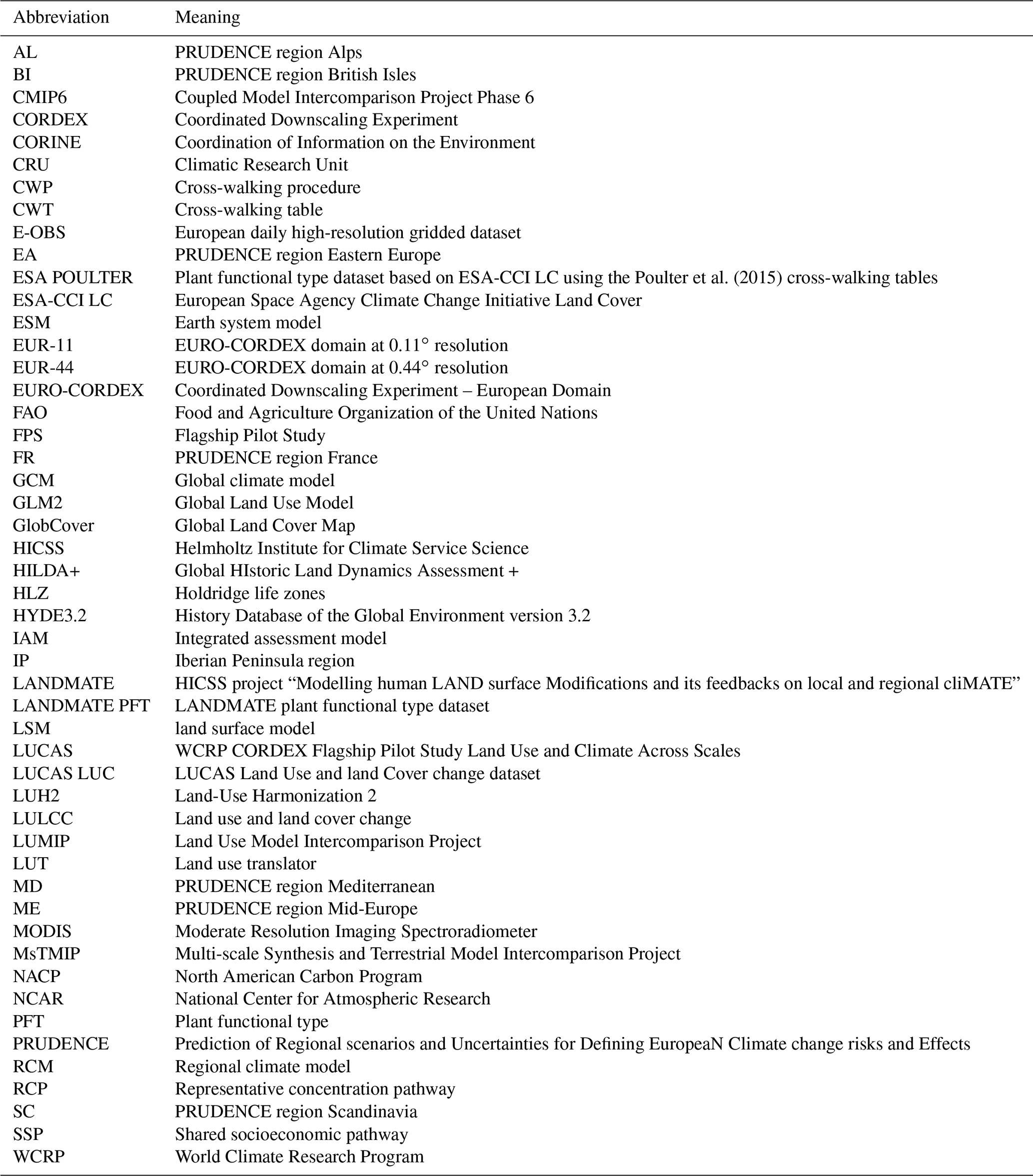
Table A2 Specification of the land use change scenarios provided by LUH2 (Hurtt et al., 2020) and the assumptions about land use and land cover developments in the different scenarios (Hurtt et al., 2020; Popp et al., 2017; Riahi et al., 2017; van Vuuren et al., 2011).

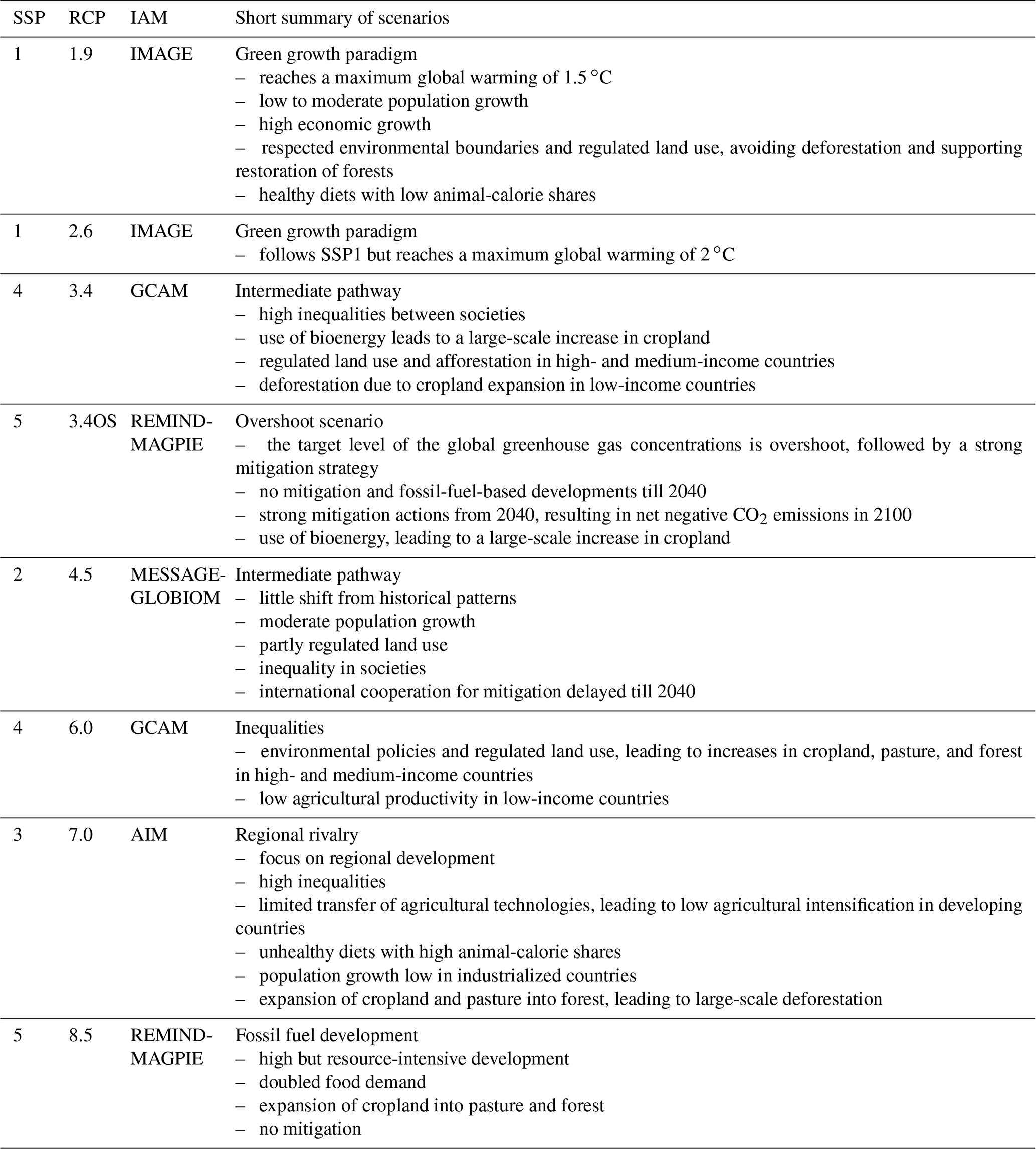
Table A3 MODIS plant functional types based on Bonan et al. (2002).

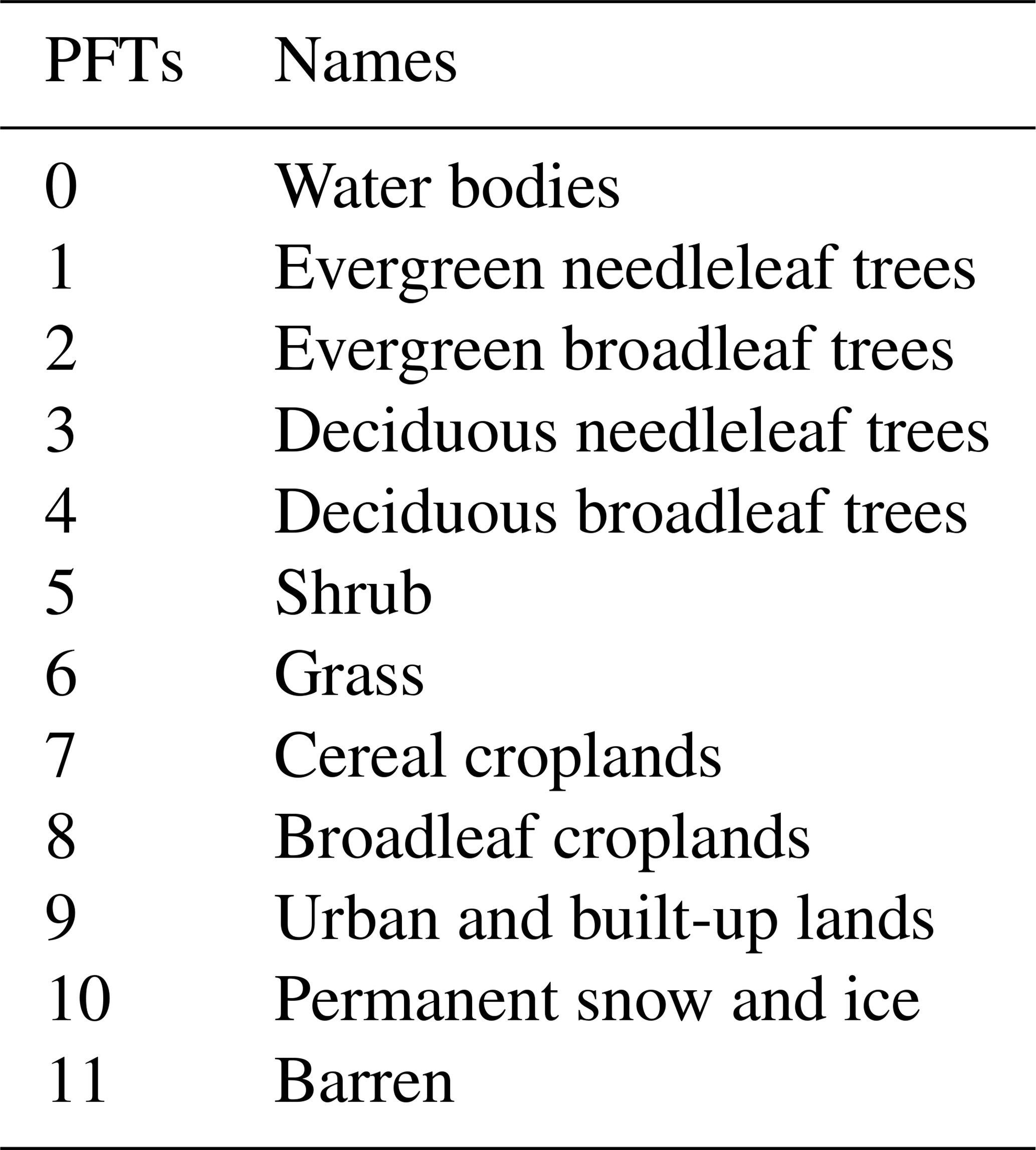
Table A4 ESA-CCI LC default cross-walking table for ESA-CCI LC class translation into ESA PFTs.

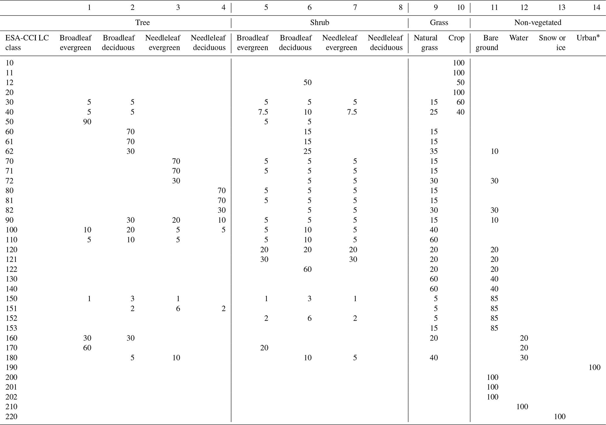
^* The urban PFT (15) was not part of the first default table provided by ESA-CCI but was added later. The urban PFT is added in this analysis for improved comparability with the other products. The urban proportion is thereby subtracted from the bare-area PFT. Since the bare areas are not part of the analysis, the influence of the urban PFT on the other proportions is negligible.