Spatially coordinated airborne data and complementary products for aerosol, gas, cloud, and meteorological studies: the NASA ACTIVATE dataset

The NASA Aerosol Cloud meTeorology Interactions oVer the western ATlantic Experiment (ACTIVATE) produced a unique dataset for research into aerosol–cloud–meteorology interactions, with applications extending from process-based studies to multi-scale model intercomparison and improvement as well as to remote-sensing algorithm assessments and advancements. ACTIVATE used two NASA Langley Research Center aircraft, a HU-25 Falcon and King Air, to conduct systematic and spatially coordinated flights over the northwest Atlantic Ocean, resulting in 162 joint flights and 17 other single-aircraft flights between 2020 and 2022 across all seasons. Data cover 574 and 592 cumulative flights hours for the HU-25 Falcon and King Air, respectively. The HU-25 Falcon conducted profiling at different level legs below, in, and just above boundary layer clouds (< 3 km) and obtained in situ measurements of trace gases, aerosol particles, clouds, and atmospheric state parameters. Under cloud-free conditions, the HU-25 Falcon similarly conducted profiling at different level legs within and immediately above the boundary layer. The King Air (the high-flying aircraft) flew at approximately ∼ 9 km and conducted remote sensing with a lidar and polarimeter while also launching dropsondes (785 in total). Collectively, simultaneous data from both aircraft help to characterize the same vertical column of the atmosphere. In addition to individual instrument files, data from the HU-25 Falcon aircraft are combined into “merge files” on the publicly available data archive that are created at different time resolutions of interest (e.g., 1, 5, 10, 15, 30, 60 s, or matching an individual data product's start and stop times). This paper describes the ACTIVATE flight strategy, instrument and complementary dataset products, data access and usage details, and data application notes. The data are publicly accessible through https://doi.org/10.5067/SUBORBITAL/ACTIVATE/DATA001 (ACTIVATE Science Team, 2020).

1 Introduction

Aerosol–cloud interactions are responsible for the largest uncertainty in estimates of total anthropogenic radiative forcing (Bellouin et al., 2020). This uncertainty stems partly from the difficulty in experimentally characterizing such interactions in the atmosphere due to the need for methods such as the use of airborne platforms. Furthermore, it is challenging to isolate the relative influence of different factors that impact the life cycle and properties of clouds, including meteorology and aerosol particles. Decades of airborne field studies focused on aerosol–cloud interactions have been limited in terms of the data volume and number of variables measured, the diversity of aerosol and weather conditions, and the vertical data coverage. These limitations motivated the conception of the NASA Aerosol Cloud meTeorology Interactions oVer the western ATlantic Experiment (ACTIVATE), which included systematic, extensive, and spatially coordinated flights with two aircraft over the northwest Atlantic (Sorooshian et al., 2019). ACTIVATE is one of five Earth Venture Suborbital-3 (EVS-3) missions.

ACTIVATE flights were strategically executed in different seasons (e.g., winter and summer) to increase the dynamic range of aerosol and meteorological conditions that resulted in different cloud types, spanning warm and mixed-phase clouds as well as the continuum from stratiform to cumulus clouds. The northwest Atlantic differs from the subtropical regions often chosen for aerosol–cloud interaction campaigns due to multiple cloud types within reach, rather than the stratocumulus clouds that are simpler to characterize owing to their high cloud fraction and well-defined vertical structure as demonstrated by campaigns over the northeast Pacific (e.g., Durkee et al., 2000; Sorooshian et al., 2018), southeast Pacific (e.g., Mechoso et al., 2014), and southeast Atlantic (e.g., Zuidema et al., 2016; Redemann et al., 2021). ACTIVATE adds to the much needed inventory of data over the northwest Atlantic to build on efforts from projects such as the North Atlantic Regional Experiment (NARE; Leaitch et al., 1996), the Surface Ocean–Lower Atmosphere Study (SOLAS; Leaitch et al., 2010), the International Consortium for Atmospheric Research on Transport and Transformation (ICARTT; Avey et al., 2007), the Two-Column Aerosol Project (TCAP), and the Investigation of Microphysics and Precipitation for Atlantic Coast-Threatening Snowstorms (IMPACTS). With a disciplined strategy of conducting the same type of flight plan for over 90 % of the flights (called “statistical surveys”), data were repeatedly collected at different vertical levels in and above the marine boundary layer, including within and immediately below and above clouds. Another subset of flights called “process studies” comprised more customized flight patterns to capitalize on targets of opportunity for remote-sensing algorithm assessments and detailed model intercomparison studies, such as wintertime cold-air outbreaks and summertime developing cumulus clouds. This rich dataset is ideal for a number of research applications including studying processes, model evaluation and improvement, parameterization development, and remote-sensing algorithm analysis and advancement.

To aid the research community in the usage of the ACTIVATE data, the goal of this work is to provide a guide for users. The structure of this paper is as follows: (i) a description of the ACTIVATE campaign and flight strategy, which involved spatial coordination between a high-flying King Air and a low-flying HU-25 Falcon; (ii) a summary of the King Air instruments and associated datasets; (iii) a summary of the HU-25 Falcon instruments and associated datasets; (iv) a description of complementary data products; (v) visualization of data products relevant to a representative case study flight; (vi) data/code availability and file format; and (vii) conclusions. To guide readers, Appendix A has a nomenclature table defining all acronyms and abbreviations used in this paper. A forthcoming paper will provide a comprehensive overview of the science results from ACTIVATE and how those fit into the larger picture of past campaigns focused on aerosol–cloud interactions.

2 Field campaign description

2.1 Objectives, operation bases, and schedule

ACTIVATE generated a novel dataset that can be used to address three overarching objectives that were developed during the conception of the mission plan: (i) quantification of the relationships amongst the aerosol particle number concentration (N_a), the cloud condensation nuclei (CCN) concentration, and the cloud droplet number concentration (N_d) as well as the reduction of uncertainty in model parameterizations of aerosol activation and cloud formation; (ii) improvement of the process-level understanding and model representation of factors that govern cloud micro/macro-physical properties and how they couple with cloud effects on aerosol; and (iii) assessment of the advanced remote-sensing capabilities with respect to retrieving aerosol and cloud properties related to aerosol–cloud interactions. To achieve these objectives, it was important to conduct a high number of flights across different seasons in order to collect sufficient statistics across a range of aerosol, cloud, and meteorological conditions for more robust calculations relevant to understanding the life cycle and properties of different types of boundary layer clouds (e.g., stratiform and cumulus as well as mixed-phase and warm clouds). To address the challenge of needing data for different vertical levels relevant to the aerosol–cloud system and to achieve remote-sensing objectives, two aircraft were employed that were kept highly coordinated in both space and time. These planes included the NASA Langley Research Center's HU-25 Falcon (low-flying aircraft, < 3 km) and King Air (high-flying aircraft, ∼ 9 km). A critical element in the selection of the two aircraft was that both aircraft flew close to 120 m s⁻¹ at their respective sampling altitudes. The flights were limited by the endurance of the aircraft (< 4 h); thus, flights were designed to try to extend the spatial range as much as possible while also still being able to characterize different vertical levels. This resulted in the approach of flying “statistical surveys” comprised of repeated “ensembles” that we describe below (Sect. 2.2) and that have been discussed in detail elsewhere for ACTIVATE flights (Dadashazar et al., 2022b).

The northwest Atlantic study region is ideal for the ACTIVATE objectives owing to the wide range of aerosol types and weather conditions (Corral et al., 2021; Painemal et al., 2021; Sorooshian et al., 2020) during the periods in which the flights took place, which ended up including November–June and August–September. Flights were mostly based out of the NASA Langley Research Center (NASA LaRC) with only a few others based out of secondary bases, including Newport News/Williamsburg International Airport (Virginia), Quonset State Airport (Rhode Island), Rhode Island T.F. Green International Airport (Rhode Island), and L. F. Wade International Airport (Bermuda). The original goal for flights was to undertake 25 joint flights in each of six deployments between 2020 and 2022, including a winter (February–March) and summer (May–June) deployment each year. As a result of operational delays, aircraft maintenance challenges, and COVID-19 emerging during the first deployment, deviations were necessary relative to the original flight schedule plan; however, the overall science plan was unaffected. These deviations are evident in Table 1, which shows a summary of flight metrics for each of the six deployments. Table 2 further summarizes each individual flight, including details specific to each aircraft, such as takeoff and landing time, and special features per flight. It is difficult to assign specific flights to ACTIVATE's individual scientific objectives (Sect. 2.1) because statistics from all flights can be helpful for each objective; however, that being said, the notes on special features and the designation of some flights as “process study” flights (described in Sect. 2) in Table 2 can be helpful for data users most interested in remote-sensing objectives (e.g., satellite underflights or relatively more cloud-free conditions with high aerosol levels) and modeling activities, such as large-eddy simulation of cold-air outbreak conditions (e.g., Li et al., 2022). Figure 1 shows the flight tracks each year for the HU-25 Falcon and King Air.

Table 1 Overall summary of the ACTIVATE flight metrics categorized by each of the six deployments between 2020 and 2022. Joint ensembles represent when both planes were coordinated and conducting the series of legs (in some combination) shown in Fig. 2. The number of dropsondes shown represents dropsondes with full profiles of all variables with good parachute performance. The threshold science mission goal for cloud ensembles required only 100 of the 200 ensembles to be joint-aircraft measurements and for the remainder to be at least with just the HU-25 Falcon. The threshold science mission represents a descoped version of the baseline mission to satisfy the minimum science acceptable for the investment, whereas the baseline mission satisfies the performance requirements necessary to achieve the full science objectives of the mission.

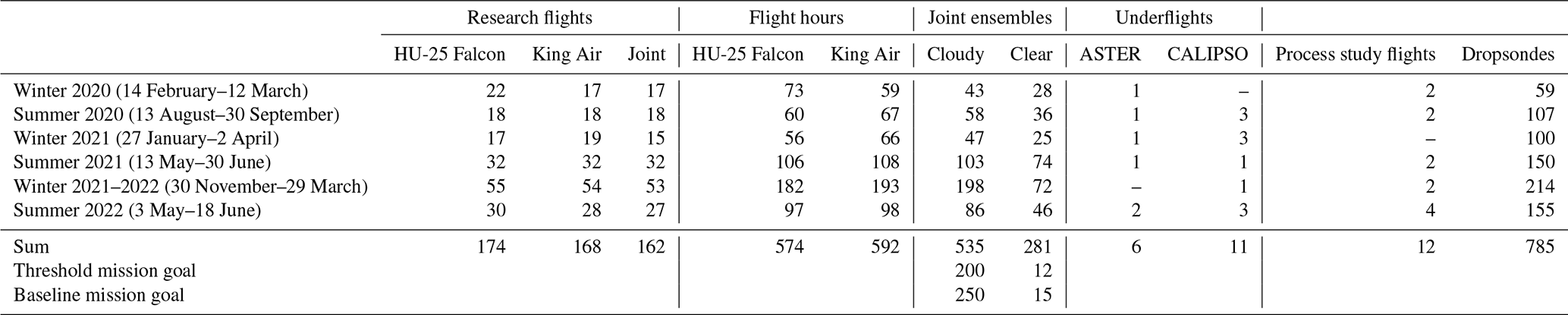
Table 2 Summary of the ACTIVATE research flights, including pertinent details associated with the date and time, and special notes. Research flights 48–61 included a reduced operational HU-25 Falcon payload due to an aircraft maintenance limitation. Deployments are separated by blank rows: deployment 1 (RF1–RF22), deployment 2 (RF23–RF40), deployment 3 (RF41–RF61), deployment 4 (RF62–RF93), deployment 5 (RF94–RF148), and deployment 6 (RF149–RF179). n/a – not applicable.

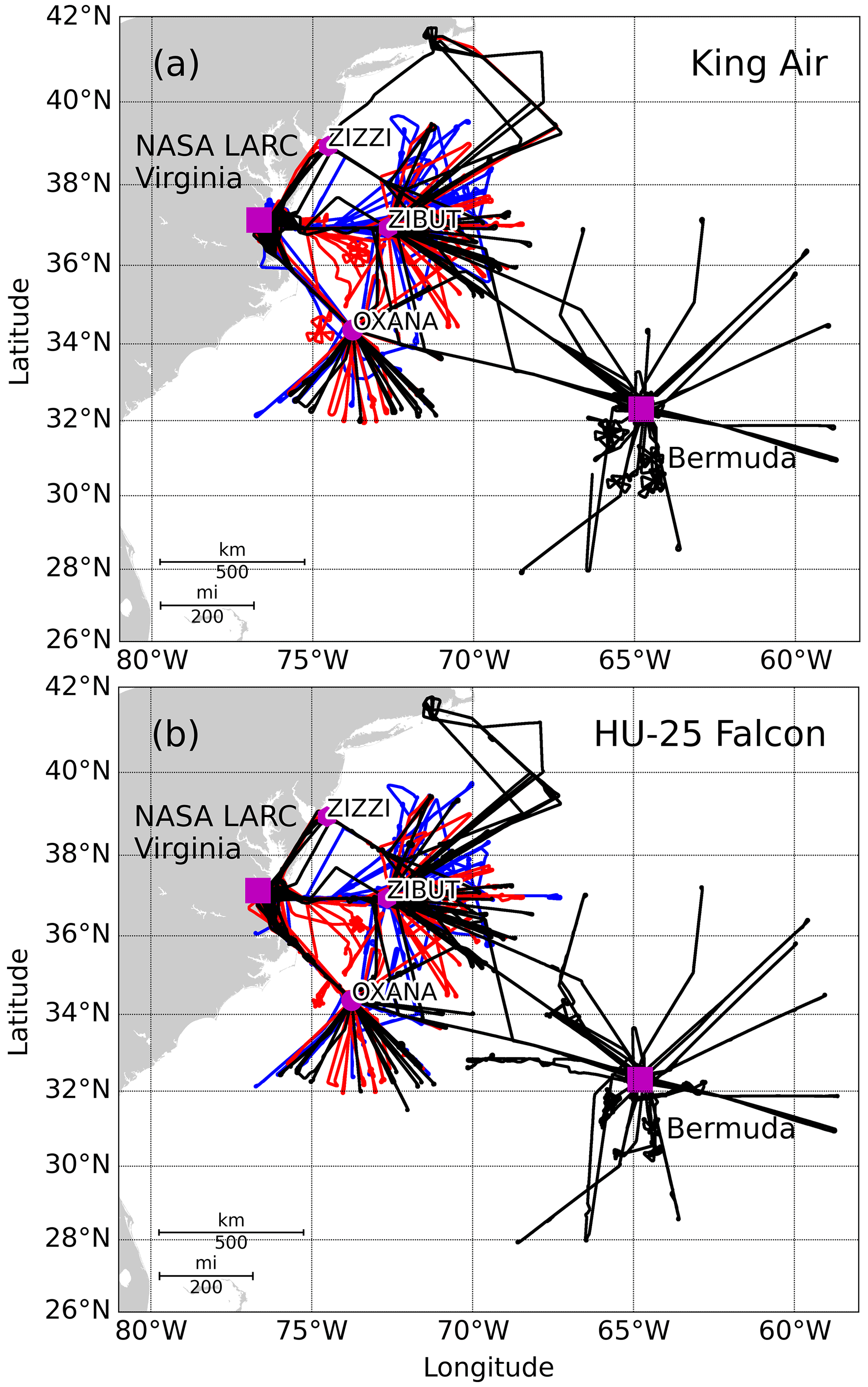
Figure 1 Flight tracks for the (a) King Air and (b) HU-25 Falcon across all 3 years of flights (blue represents 2020, red represents 2021, and black represents 2022). ZIBUT and OXANA are two waypoints used in most flights to adhere to air traffic control restrictions, whereas ZIZZI was less commonly used.

2.2 Flight strategy

The original goal of ACTIVATE was to allocate 90 % of the flights to “statistical surveys”, during which the two aircraft would repeatedly conduct coordinated cloud and cloud-free ensembles (Fig. 2). The threshold and baseline science mission success metrics from a flight perspective hinged on acquiring many of these ensembles for more robust calculations of aerosol–cloud–meteorology interactions. ACTIVATE far surpassed the number of ensembles needed for threshold and baseline mission requirements. The ensemble numbers and definitions of these mission categories are provided in Table 1. Cloud ensembles performed by the low-flying HU-25 Falcon aircraft included flying level legs (∼ 3 min each unless otherwise dictated by flight conditions) in the following nominal order: below cloud base (BCB), above cloud base (ACB), a second pair of BCB and ACB, minimum altitude (MinAlt), above cloud top (ACT), and below cloud top (BCT). MinAlt is defined as the lowest altitude that the aircraft could fly at, which was ∼ 150 m a.s.l. (above sea level) when clear of cloud and operating under good-visibility conditions. The slant ascents from MinAlt to ACT provided multiple in situ vertical profiles across the range of relevant altitudes and included periods of cloudy and cloud-free sampling depending on conditions. A caveat to the interpretation of these “vertical” profiles is that, in environments with spatially varying conditions (e.g., broken or episodic cloud), the slant ascent may not represent average conditions with any reliability. Clear ensembles under cloud-free conditions included legs in the following nominal order: MinAlt, above boundary layer top (ABL), below boundary layer top (BBL), and a remote-sensing (RS) leg. The RS leg was implemented under conditions of high aircraft coincidence (< 5 min and < 6 km of separation between the HU-25 Falcon and King Air) and when no clouds affected the field of view. The RS leg provided a second low-altitude leg (∼ 230 m) to help with lidar extinction comparison in the challenging near-surface region. The altitude of the ABL leg was estimated by flight scientists based on gradients in the available real-time data during ascents and descents. Occasionally deviations that required changes in altitude occurred in these leg orders for both ensemble types due to atmospheric conditions and air traffic control challenges. The time span (distance) of each leg and cloud ensemble was ∼ 3.3 min (∼ 24 km) and ∼ 35 min (∼ 250 km), respectively, whereas clear ensembles were typically ∼ 15 min (∼ 100 km) (Dadashazar et al., 2022b). Across 162 final joint flights, all but 12 were classified as statistical surveys (93 %), with the classification of each flight shown in Table 2. An archived forward-facing camera video from the HU-25 Falcon on a representative statistical survey flight is accessible (https://asdc.larc.nasa.gov/news/activate-data-webinar-materials, last access: 24 July 2023) to show data users how the ensembles appeared visually from the perspective of the aircraft. A representative statistical survey flight is discussed in more detail in Sect. 6.

The disciplined approach of statistical surveys is uncommon for airborne flight projects, as the temptation is often to target the most interesting features on a given day, such as the strongest aerosol signal (e.g., smoke or dust plume) or opportunistic experimental conditions suited for aerosol–cloud interactions (e.g., ship tracks) (e.g., Christensen et al., 2022). Building routine statistics below, within, and above boundary layer clouds with a consistent flight strategy across a large number of flights is advantageous for developing probability density distributions of aerosol, cloud, and meteorological properties in a given region, which can be used to trace back onto processes. Furthermore, this approach provided a consistent dataset to better optimize data use among a diverse set of users.

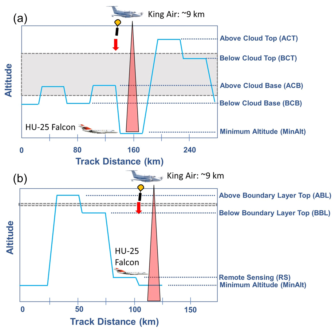
Figure 2 Panel (a) shows the nominal flight pattern constituting a “cloud ensemble” as part of the ACTIVATE flights, whereby the HU-25 Falcon conducts stairstepping (shown using light blue lines) at various levels (∼ 3 min each usually) below, in, and immediately above boundary layer clouds. Note that MinAlt represents the lowest altitude that the HU-25 Falcon could operationally fly at (∼ 150 m a.s.l.). The King Air flies overhead at around ∼ 9 km. The gray shaded area represents a cloud. Typical statistical survey flights included approximately three cloud ensembles. Panel (b) presents the nominal flight pattern for “clear ensembles”, whereby the HU-25 Falcon stairsteps at levels immediately above and below the boundary layer top (represented by the horizontal gray bar), and legs near the HU-25 Falcon's lowest operational altitude. The remote-sensing leg was an additional leg just above the MinAlt leg to facilitate data comparisons between the in situ HU-25 Falcon instruments and the King Air remote sensors very near the ocean surface. The vertical axes are compressed to show both aircraft.

The remaining 10 % of flights were intended to be “process study” flights, with their number reduced to 12 out of 162 (7 %) in practice. The goal of these flights was to focus on a target of opportunity, thereby providing a more detailed characterization of the specific location of a particularly interesting cloud scene. A total of 4 of the 12 process studies were conducted during wintertime cold-air outbreak events, with the remaining 8 focused on summertime cumulus cloud fields. These flights typically entailed a more detailed vertical characterization of the atmospheric column in which the HU-25 Falcon was conducting stacked legs below, in, and above clouds (often termed a “wall” pattern), with bounding vertical soundings at the beginning and end of the wall(s). During that time, the high-flying King Air would conduct a carefully designed module at high altitude to maximize coordination as well as to provide detailed information about the scene encompassing the clouds of interest. For example, during some winter process studies, the King Air conducted a large circle aloft with numerous dropsonde launches to derive relevant quantities such as divergence profiles and surface fluxes to be used for model intercomparison studies (Chen et al., 2022; Seethala et al., 2021; Li et al., 2022). A visual representation of a generic process study flight is shown in Fig. 3. Note that the aircraft would still conduct ensembles (Fig. 2) within process study flights; these took place during transits to and from the key area of focus where a wall pattern would be conducted.

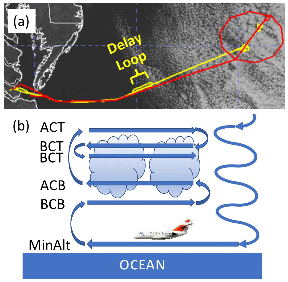
Figure 3 Panel (a) presents a visual summary of Research Flight 13 (1 March 2020, L1) tracks for both the (yellow) HU-25 Falcon and (red) King Air overlaid on GOES-16 imagery (15:21 UTC). Highlighted in the flight is a “delay loop” (described in Sect. 2.4) executed by the HU-25 Falcon to improve coordination with the King Air. Panel (b) shows the generic HU-25 Falcon pattern used in process study flights, including stacked level legs (wall) with spiral soundings before and after the wall; meanwhile, the King Air (not shown in panel b) flew aloft characterizing the same area. During this flight, in place of a spiral sounding at the end of a wall, the HU-25 Falcon conducted a slant descent from the last BCT leg to a subsequent MinAlt leg.

2.3 Recommended terminology

The following guidelines are encouraged when reporting information about specific flights based on information in Table 2. References should provide the RF number and date. In cases where two flights occurred on a given day, one can additionally include “L1” or “L2” to signify launch 1 or 2, respectively. Note here that the launch number refers to the aircraft launch number per day following the ICARTT (described further in Sect. 7) naming convention (Northup et al., 2017), not to the processing level as employed by the satellite and remote-sensing community. As each flight has a unique RF number, the launch number only becomes more important if the flight dates are used without reference to the RF number. Therefore, examples include the following: “RF1 (14 February 2020)”; “RF6 (22 February 2020)” or “22 February 2020, L2”. Furthermore, it is encouraged to refer to the six deployments according to their season and year for simplicity (e.g., Winter 2020, Summer 2020, Winter 2021, Summer 2021, Winter 2022, and Summer 2022) as shown in Table 1, with the caveat that the Winter 2022 deployment still includes November–December flights occurring in 2021. This is encouraged for simplicity, even though the months of flights do not perfectly align with typical seasonal definitions (e.g., DJF is winter and JJA is summer).

2.4 Special flight details

A few special features that impacted flight execution are worth expanding upon:

• Single-aircraft flights (17 in total) were conducted when one of the aircraft was grounded, usually as the result of a maintenance issue. In rare cases, such as RF177 (16 June 2022), both planes began a joint flight, but one plane (the HU-25 Falcon in this case) experienced a maintenance issue during flight and returned to base without any science data archived. This meant that the flight qualified as a single-aircraft flight, as only the King Air obtained archivable data. For single-aircraft HU-25 Falcon flights, statistical surveys were usually conducted with one process study flight; RF163 on 2 June 2022 was a unique process study flight in that it was conducted with the HU-25 Falcon alone and involved wall patterns. The King Air also conducted its usual flight strategy during single-aircraft flights, flying aloft at ∼ 9 km and sampling targets of opportunity that were deemed to be too important to miss, even in the absence of the HU-25 Falcon, such as cold-air outbreaks (e.g., RF42 on 29 January 2021).

• Flights based out of either NASA Langley Research Center or Newport News/Williamsburg International Airport almost always included transits to one of two waypoints – ZIBUT (36.938^∘ N, 72.666^∘ W) or OXANA (34.363^∘ N, 73.759^∘ W) – in order to adhere to strict air traffic control restrictions; farther offshore there was more flexibility for waypoint selection. Those two waypoints can be thought of as “pivot points” that are visually evident and labeled in Fig. 1. A few flights included transits from one of the two Virginia bases to the northeast to waypoint ZIZZI (38.941^∘ N, 74.529^∘ W; shown in Fig. 1) to strategically sample upwind conditions during cold-air outbreaks. Due to the limitations associated with the COVID-19 pandemic during the first four deployments (2020–2021), secondary bases for the purpose of extending ACTIVATE's spatial range were only used in deployments 5 and 6 in 2022.

  Notable was a series of flights based in Bermuda in June 2022 to make up for not flying there earlier in the campaign. The rationale for data collection around Bermuda was multifold. Firstly, this area was farther removed from continental pollution sources and, thus, more closely resembled a remote marine aerosol regime. Secondly, the aforementioned conditions simplify parsing out causal drivers of aerosol–cloud interactions (e.g., less impacted by terrestrial boundary layer and Gulf Stream effects). The coastal region by the mid-Atlantic states has a strong air mass disequilibrium (e.g., high air–sea contrasts), but air masses relax to a more (quasi-)steady state farther downwind, which has more global relevance than coastal regions. Thirdly, data collection in this region could connect aircraft measurements with long-term surface measurements conducted at Bermuda (Sorooshian et al., 2020), including notable long-term aerosol and precipitation datasets collected through the Bermuda Institute of Ocean Sciences (BIOS) with demonstrated utility for ACTIVATE, as shown in recent studies (Aldhaif et al., 2021; Dadashazar et al., 2021a). Finally, data collection in this region could also bridge the gap for aerosol–cloud studies carried out under polluted conditions vs. the low-CCN conditions observed during missions like the North Atlantic Aerosols and Marine Ecosystems Study (NAAMES; Behrenfeld et al., 2019) and the Aerosol and Cloud Experiments in the Eastern North Atlantic (ACE-ENA; Wang et al., 2022).

• Numerous flights were coordinated with satellite overpasses to achieve remote-sensing objectives. A total of 6 and 11 of these “underflights” of satellites were conducted in coordination with the Advanced Spaceborne Thermal Emission and Reflection Radiometer (ASTER) and Cloud-Aerosol Lidar and Infrared Pathfinder Satellite Observations (CALIPSO) missions, respectively. In a few instances, the two aircraft coordinated to observe aerosol particles under clear-sky conditions using the complete set of remote-sensing polarimeter and lidar instruments with a matching full vertical profile of in situ observations; this is related, in part, to past attempts to undertake such coordinated maneuvers in other regions (Xu et al., 2021). This type of aircraft observation module, which must include an ascent–descent or spiraling aircraft pattern by the in situ aircraft, became known as “unicorn aerosol modules”. This name stuck thanks to the artwork of a team member's elementary school child. These modules included the HU-25 Falcon conducting a vertical spiral sounding with a slower climb rate (2–5 m s⁻¹) from its lowest possible altitude (usually ∼ 120–150 m) to usually upwards of 5 km to reach the ceiling of high aerosol loadings while the King Air flew aloft, as it normally did. These modules targeted cloud-free scenes with relatively high aerosol concentrations to address aerosol optical and microphysical property remote-sensing objectives, with a demonstration of results reported by Schlosser et al. (2022). Examples are associated with RF28 (26 August 2020), RF29 (28 August 2020), RF130 (2 March 2022), RF131 (3 March 2022), RF144 (26 March 2022), and RF155 (17 May 2022). Although not labeled as unicorn modules in Table 2, several spiral profiles were conducted with the HU-25 Falcon just offshore of the Tudor Hill Marine Atmospheric Observatory during the set of Bermuda flights in June 2022 with the King Air flying overhead; these profiles sometimes included cloud (e.g., RF169 on 8 June 2022 and RF178 on 17 June 2022) and were farther removed from the polluted eastern coast of the US. However, African dust was present during some of these cases and, thus, may interest some data users. Examples of Tudor Hill spirals with King Air overpasses are seen in RF166, RF167, RF169, RF170, RF172, RF174, RF175, and RF178 (dates shown in Table 2). The Tudor Hill site, managed by BIOS, was used during the June 2022 deployment for extensive surface and tower measurements relevant to atmospheric chemistry as part of the Bermuda boundary Layer Experiment on the Atmospheric Chemistry of Halogens (BLEACH).

• The HU-25 Falcon experienced a significant maintenance issue at the completion of RF47 (21 February 2021), resulting in a reduced instrument payload for the remainder of the Winter 2021 deployment (RF48–RF61, from 4 March to 2 April 2021). The following instruments (described in Sect. 4) were not allowed to operate or collect data in order to minimize electrical power demand: trace gases (Picarro, 2B Tech.), the aerosol mass spectrometer (AMS), the particle-into-liquid sampler (PILS), and the counterflow virtual impactor (CVI). The 11 d gap between RF47 and RF48 (4 March 2021) was due to the adaptation of the HU-25 Falcon aircraft to the new payload strategy. To make up for most of the Winter 2021 flights not having a full payload capability, the Winter 2022 deployment was essentially the equivalent of two deployments, with flights starting as early as 30 November 2021 and ending on 29 March 2022 (55 total flights, rather than the nominal 25). No research flights occurred from 10 December 2021 to 11 January 2022 in order to observe the winter holiday period.

• Effort was made to keep the two aircraft as spatially coordinated as possible throughout the 162 joint flights. This was challenging at times due to pronounced differential wind speeds (and direction) between the boundary layer (HU-25 Falcon) and ∼ 8–10 km altitude (King Air) as well as due to unforeseen delays in takeoff for the second aircraft on a given day, typically due to the airfield operations. The goal was to try to keep the aircraft within approximately 5 min and 6 km of each other. This goal was attained for ∼ 73 % of the dataset. If one aircraft was too far ahead, it would often conduct a “delay loop” (i.e., racetrack), whereby it would fly in a reverse track until the other aircraft caught up and then turn around again and fly in joint fashion. An example is shown in Fig. 3a for RF13 (1 March 2020, L1). Sometimes the trailing aircraft would turn around sooner at the “turn point” of an out-and-back flight to help reduce the spacing.

3 King Air measurements

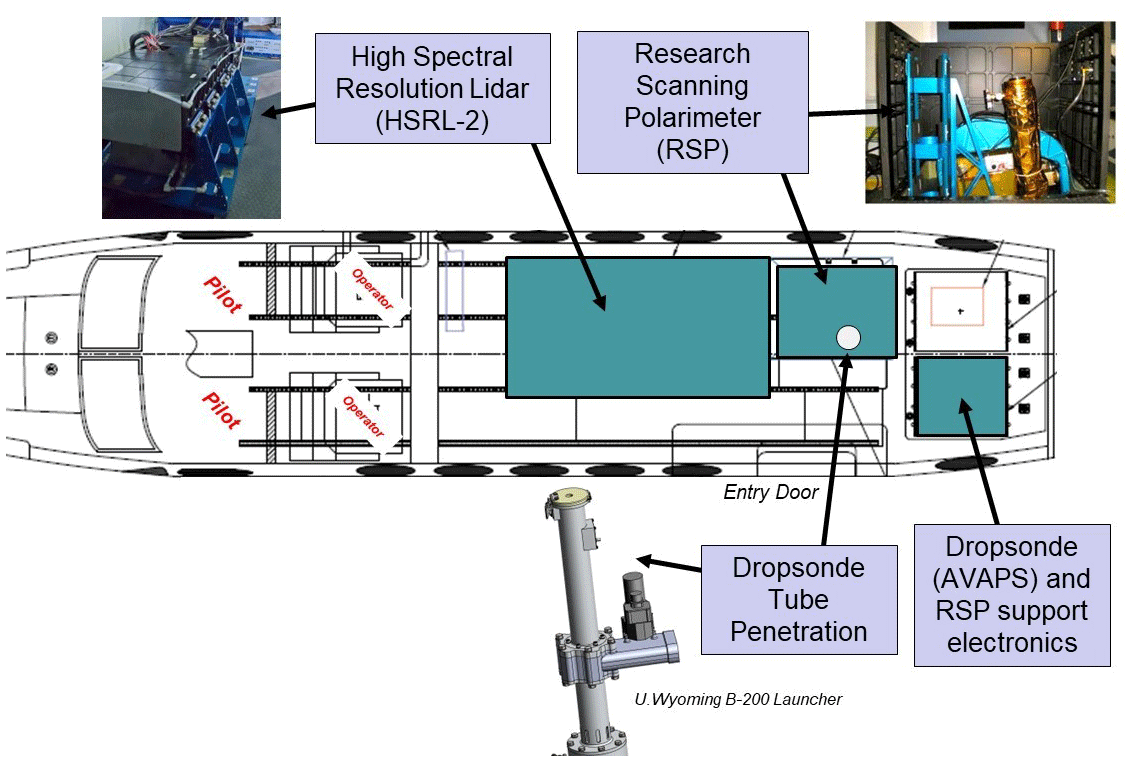
Two separate King Air aircraft were used during the campaign, with nearly identical flight performance characteristics. The science payload was moved from the King Air with the tail number N528NA (UC-12) to a second King Air with the tail number N529NA (B200) for RF94–RF119 to accommodate science flights during a planned maintenance period on N528NA. All other King Air research flights were flown using N528NA. Table 3 summarizes the King Air payload along with measured variables from each instrument and their associated uncertainties and resolutions. Figure 4 shows a visual summary of the interior King Air layout. Table S1 in the Supplement summarizes the performance of each instrument on both aircraft for each flight to aid data users requiring at least some minimum combination of functional instruments for their applications. Each instrument package is described in detail below.

Table 3 Summary of the King Air instrumentation and measurements. Products under development are omitted from this table; readers are referred to Sect. 3 for more information. n/a – not applicable.

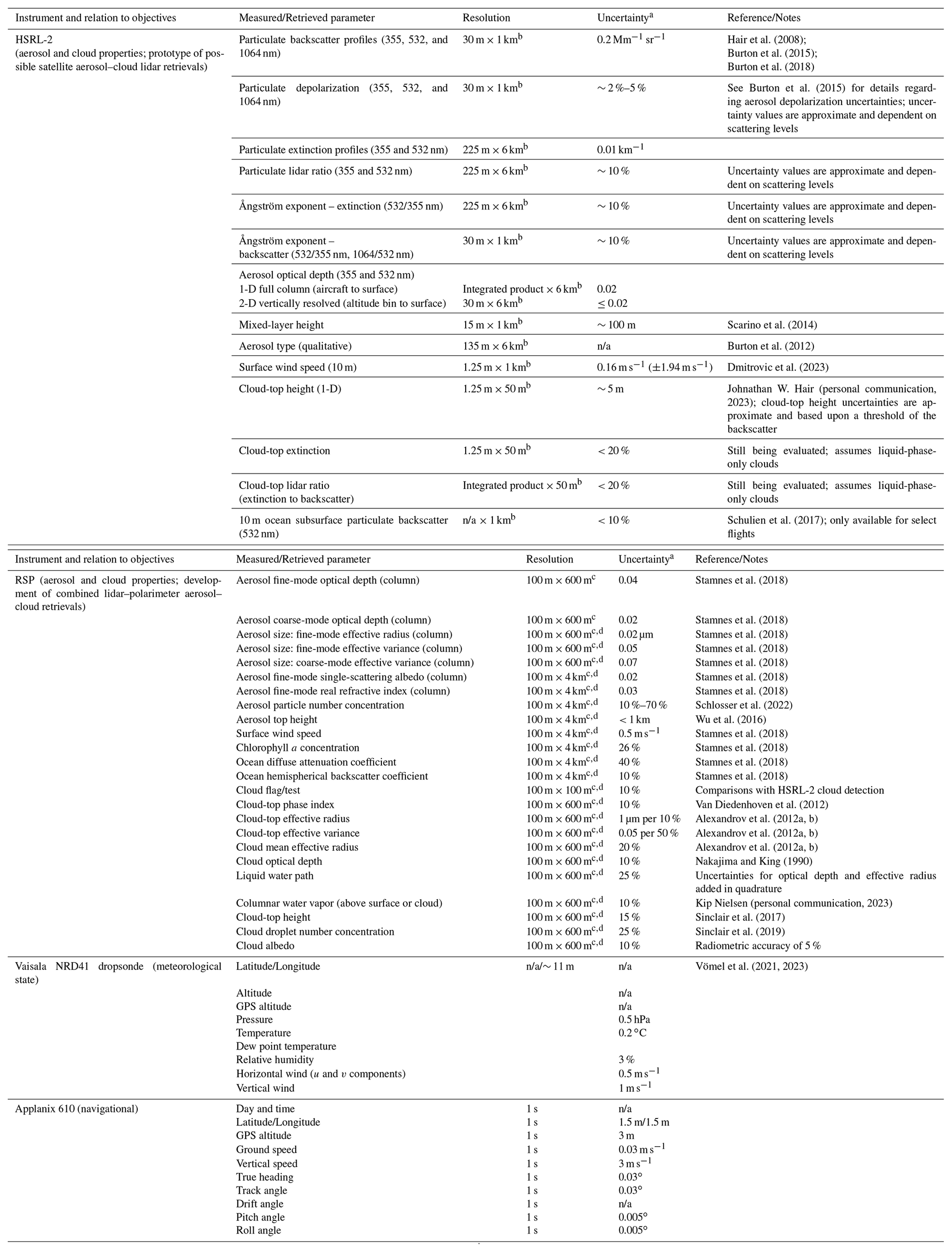
^a Uncertainties, which represent a combination of measurement precision and accuracy, are presented for typical measurement conditions. ^b “x m/y m” indicates x m vertical resolution and y m horizontal resolution along the track. ^c Cross-track by along-track resolution. ^d Non-imaging: along-track product with single cross-track elements for the research scanning polarimeter (RSP).

Figure 4 The King Air interior layout.

3.1 Applanix navigational data

For basic navigational and aircraft motion information, an Applanix 610 system acquired 1 s data for calendar day, time, latitude, longitude, GPS altitude, ground speed, vertical speed, true heading, and track, drift, pitch, and roll angle.

3.2 High Spectral Resolution Lidar – generation 2 (HSRL-2)

The NASA Langley High Spectral Resolution Lidar (HSRL-2) is a multiwavelength airborne HSRL providing vertically resolved extensive and intensive aerosol properties. Extensive properties are those that depend on both aerosol particle properties and concentration, whereas intensive properties depend only on the particle properties and are independent of concentration. Archived HSRL-2 core data include high-resolution profiles of particulate backscatter and depolarization at three wavelengths (355, 532, and 1064 nm) and simultaneous and independent measurements of particulate extinction at two wavelengths (355 and 532 nm) via the HSRL technique (Hair et al., 2008; Burton et al., 2018). These profiles are used to derive horizontally and vertically resolved curtains of the extinction and backscatter Ångström exponent, the lidar ratio (i.e., extinction-to-backscatter ratio), the backscatter Ångström exponents for spherical and nonspherical particles (dust and crystalline sea salt) (Sugimoto and Lee, 2006), and the aerosol type (Burton et al., 2012). Cloud screening is performed using a convolution of the measured 532 nm signal with a Haar wavelet to enhance edges (Davis et al., 2000) by separating the sharper cloud edges from less pronounced aerosol features in each lidar profile. Cloud-top altitudes are provided. Both the cloud-screened and non-cloud-screened aerosol scattering ratio (i.e., ratio of aerosol scattering to molecular scattering), aerosol backscatter, and aerosol depolarization profiles are computed and provided at the three wavelengths. Aerosol extinction, aerosol optical thickness, and the lidar ratio at 355 and 532 nm are provided only for cloud-free regions. If a cloud is detected in a profile, these data products are restricted to the region above the cloud top. The 532 nm molecular scattering signal for each profile is used to check that signal levels are sufficiently high to derive these aerosol products. Aerosol depolarization at 532 and 1064 nm (355 nm) is computed when the aerosol scattering ratio values exceed 0.2 (0.068). The HSRL-2 backscatter and depolarization products are reported as 10 s averages, whereas the extinction and lidar ratio products are averaged to 60 s. Higher-resolution products are available from the HSRL-2 team upon request. The aerosol backscatter product is also used to derive an aerosol mixed-layer height (MLH) (Fast et al., 2012; Scarino et al., 2014). Mixed-layer heights are based on sharp gradients in aerosol backscatter profiles that are found using a modified Haar wavelet approach (Scarino et al., 2014). The MLH remains challenging to accurately determine under complex atmospheric conditions, such as shallow marine boundary layers (MBLs) and multiple aerosol layers as a function of altitude. There are many ways that the MLH can be defined and retrieved; thus, users should use discretion in how they use MLH data for their given applications. Aerosol typing (maritime, polluted maritime, pure dust, dusty mix, smoke, fresh smoke, urban, and ice) is based on an algorithm using depolarization, depolarization wavelength dependence, aerosol backscatter wavelength dependence, and the aerosol lidar ratio (Burton et al., 2012).

Within ACTIVATE, additional new HSRL-2 geophysical products have been developed (or are under development), including an aerosol hygroscopic growth parameter for well-mixed MBLs, 10 m surface wind speeds, several cloud products, and an in-ocean backscatter product. A new product that is under development is the aerosol hygroscopic growth parameter f(RH), which is produced using the HSRL-2 aerosol backscatter product and state parameters retrieved from the Airborne Vertical Atmospheric Profiling System (AVAPS) dropsonde system (Sect. 3.5) in well-mixed MBLs (Richard A. Ferrare, personal communication, 2023). The 10 m neutral stability (U10) surface wind speeds are estimated using HSRL-2 retrievals of sea surface backscatter, i.e., the reflectance of the transmitted laser pulses from the ocean surface (Dmitrovic et al., 2023). The surface backscatter, retrieved with a 1.25 m vertical resolution that corrects for ocean subsurface scattering, is highly correlated with sea surface wave slope variance, which is then related to wind speed through various empirical relationships (Cox and Munk, 1954; Hu et al., 2008). New HSRL-2 cloud retrieval products include cloud-top height, cloud-top extinction, and the cloud-top lidar ratio at horizontal resolutions of 75, 150, and 150 m, respectively (Johnathan W. Hair, personal communication, 2023). Relevant to ocean–air interactions, such as marine biogenic emissions (Corral et al., 2022a), ocean subsurface particulate backscatter coefficients at 532 nm are estimated at a depth of 10 m (Schulien et al., 2017) and made available for selected flights.

Figure 5 provides a visualization of many of the aforementioned HSRL-2 data products for a representative flight (RF157 on 18 May 2022). Figure 5a shows profiles of aerosol backscatter (532 nm) for the entire flight from Bermuda to NASA LaRC in southeastern Virginia. Note the horizontal and vertical variability in the aerosol particles throughout the flight. The labeled boxes in Fig. 5a indicate regions where subsets of HSRL-2 data products are shown in the corresponding small boxes in Fig. 5b, c, and d; these are shown for clouds (Fig. 5b), boundary layer and lower-troposphere aerosols (Fig. 5c), and an elevated aerosol layer (Fig. 5d). These small boxes provide brief visualizations of these various data products. Blue dots in Fig. 5b show (left subplot) cloud-top height and (right subplot) cloud-top extinction, averaged over the first optical depth, for this region. Figure 5c shows HSRL-2 products including mixed-layer height (blue dots), surface wind speed (black line), aerosol type, aerosol depolarization (UV, 355 nm; VIS, 532 nm; IR, 1064 nm), and the backscatter Ångström exponents corresponding to spherical and nonspherical particles (dust and crystalline sea salt) in the boundary layer and lower troposphere. Figure 5d shows HSRL-2 products in the aerosol layer between 4.5 and 6.5 km, including aerosol backscatter (UV, 355 nm; VIS, 532 nm; IR, 1064 nm), the backscatter Ångström exponents (VIS $/$ UV and IR $/$ VIS), lidar ratios (UV and VIS), aerosol extinction (UV and VIS), the extinction Ångström exponent (UV $/$ VIS), and total column aerosol optical thickness (AOT; UV and VIS) (indicated by the blue and green lines in the bottom subpanel of Fig. 5d).

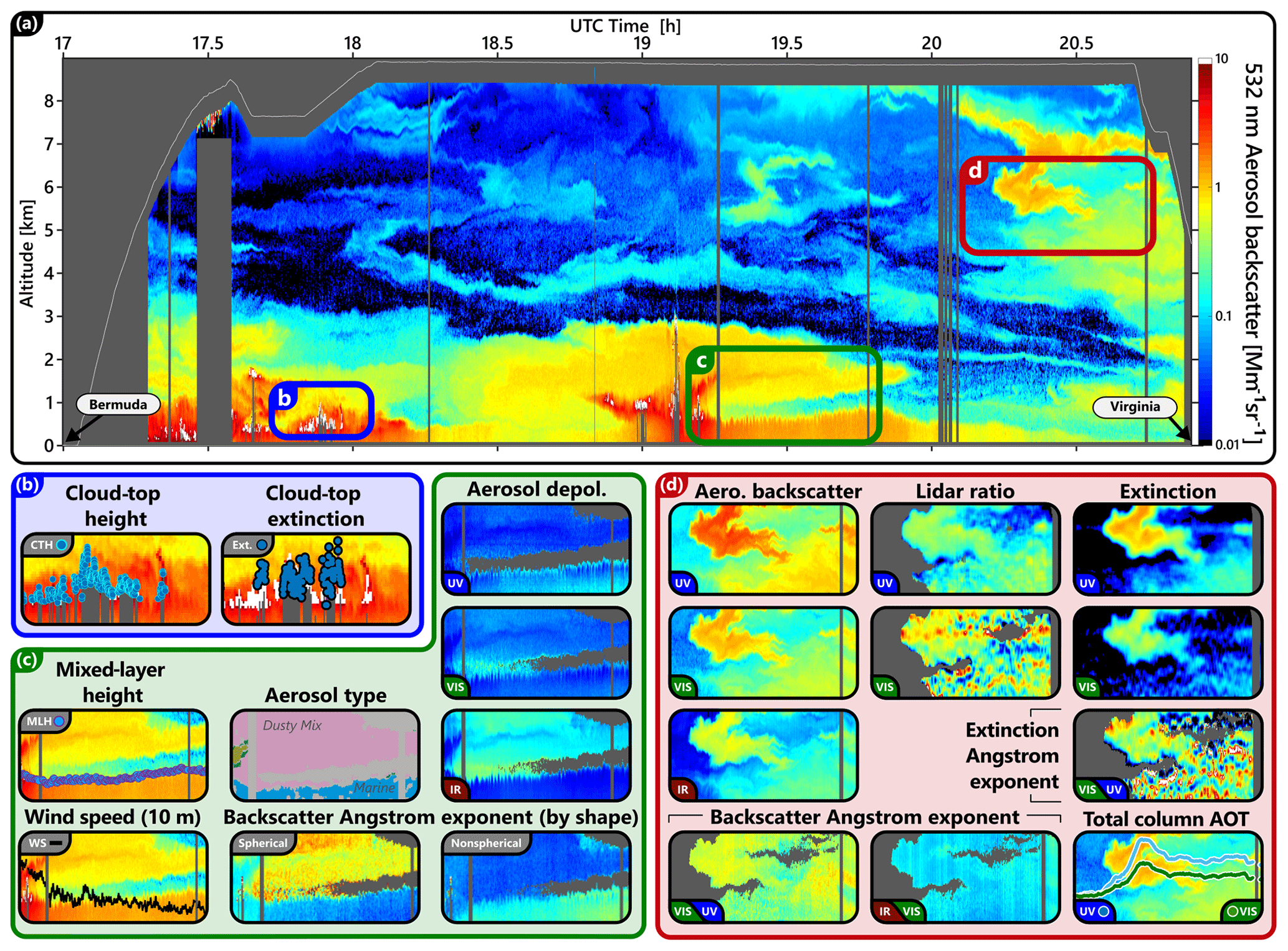
Figure 5 A qualitative visualization of selected HSRL-2 data products archived for a representative ACTIVATE flight (RF157 on 18 May 2022, L2). This flight was the second one on this day, returning from Bermuda to NASA LaRC. (a) A curtain vertical profile of aerosol backscatter (532 nm) as a function of UTC time for the entire flight provides context for the aerosol particles measured. The labeled boxes indicate regions where subsets of HSRL-2 data products are highlighted in the corresponding small boxes below panel (a). Panel (b) presents cloud data: blue dots show (left) cloud-top height and (right) cloud-top extinction, averaged over the first optical depth; both are overlaid on the backscatter curtain at the same times, with extinction being plotted on a secondary y axis (not shown). Panel (c) shows the mixed-layer height (blue dots), surface wind speed (black line), aerosol type, aerosol depolarization (UV, 355 nm; VIS, 532 nm; and IR,1064 nm), and backscatter Ångström exponents corresponding to spherical and nonspherical particles for boundary layer and lower-troposphere aerosol particles. Panel (d) presents the aerosol backscatter (UV, 355 nm; VIS, 532 nm; and IR, 1064 nm), backscatter Ångström exponents (VIS $/$ UV and IR $/$ VIS), lidar ratios (UV and VIS), aerosol extinction (UV and VIS), extinction Ångström exponent (UV $/$ VIS), and total column AOT (UV and VIS) for the elevated aerosol layer. The opaque cloud average extinction, surface wind speed, and total column AOT products are all overlaid on the backscatter curtains for context, but they are plotted on a secondary y axis and scaled for visibility inside the inset.

3.3 Research scanning polarimeter (RSP)

Retrievals of aerosol, cloud, and surface reflectance properties were provided by the research scanning polarimeter (RSP), which is a passive, downward-looking polarimeter with nine spectral bands (band centers at 410, 470, 550, 670, 865, 960, 1590, 1880, and 2260 nm) that scans its 14 mrad instantaneous field of view (∼ 100 m) along the King Air ground track (Cairns et al., 2003). Each RSP scan views the Earth over an angular range of ±55^∘ from nadir (∼ 140 views) every 0.8 s, providing radiance and linear polarization measurements in all nine spectral bands. Each scan includes stability, dark reference, and calibration checks. A few decisions with respect to flight planning and execution aimed to enhance RSP data quality, including the following: (i) keeping the aircraft stable as much as possible (e.g., yaw and roll); (ii) unless there was a high-priority reason to fly under cirrus clouds, plan the typically joint flights for days with minimal cirrus clouds forecast above the flight track in order to allow for more accurate determination of the incoming solar radiation; and (iii) fly as close as possible to the solar principal plane (i.e., azimuthally toward or away from the Sun), based on the scientific benefits of observing sunglint and maximizing the range of scattering angles observed, including in the range from 135 to 165^∘ for the polarimetric cloud bow retrievals. The public data archive contains README files provided by the RSP team for their Level-1C and Level-2 cloud and aerosol products, including important details about biases and uncertainties, that data users should consult.

Because of the scanning nature of the RSP, whereby it views areas behind and ahead of the plane, data are reordered in archived Level-1C files such that, rather than being ordered according to time, the data are sorted so that all the viewing angles that see the same nadir scene are put together. For cloudy and cloud-free scenes, this amounts to data being aggregated to the cloud top and surface, respectively. Data from the Level-1C files are then used to develop Level-2 data files housing the aerosol and cloud data variables shown in Table 3. The RSP is ideally suited for characterizing warm-cloud properties owing to the high angular density of observations per scene, with the polarized observations of the cloud bow allowing the retrieval of information about the droplet size distribution and also the detection and characterization of drizzle (Alexandrov et al., 2012b). Spectral bands in the regions where liquid and ice absorb (1.59 and 2.26 µm, respectively) also allow the RSP to obtain bi-spectral retrievals of droplet sizes, using the same technique as applied to satellite instruments such as the Moderate Resolution Imaging Spectroradiometer (MODIS) and the Visible Infrared Imaging Radiometer Suite (VIIRS). The primary cloud properties retrieved include cloud flag/test, cloud-top altitude, cloud-top phase index, cloud optical thickness, and cloud droplet size distribution (i.e., effective radius and variance). The cloud flag/test indicates whether a cloud was detected underneath the aircraft. A multi-angle parallax approach is used to estimate cloud-top heights (Sinclair et al., 2017). The cloud-top phase index variable indicates whether there is liquid at cloud top (van Diedenhoven et al., 2012). Multi-angle polarimetry is used to retrieve the effective radius and variance of the drop size distribution at cloud top for both liquid and mixed-phase clouds (Alexandrov et al., 2012b, a) and, for observations close to the solar principal plane, the drop size distribution itself (Alexandrov et al., 2012b, a). These multi-angle polarimetric retrievals have been validated against in situ observations (Adebiyi et al., 2020; Alexandrov et al., 2018) and found to be much more robust against artifacts than bi-spectral retrievals (Fu et al., 2022). Bi-spectral retrievals were also conducted for effective radius and cloud optical thickness (Nakajima and King, 1990). The column water vapor amount is provided above either the surface (cloud-free scenes) or cloud top (cloudy scene) (Sinclair et al., 2019).

Level-2 aerosol products (Stamnes et al., 2018; Schlosser et al., 2022) for both the fine and coarse mode include aerosol optical depth, aerosol size distribution parameters (effective radius/variance and number concentration), single-scattering albedo (SSA), and the real part of the refractive index; moreover, ocean properties (ocean diffuse attenuation coefficient, ocean hemispherical backscatter coefficient, chlorophyll a concentration, and surface wind speed) are reported in these files based on a model for open-ocean waters (Chowdhary et al., 2006). An aerosol layer height is also retrieved from the RSP observations (e.g., Wu et al., 2016), but we note that the HSRL-2 sensor provides far greater detail regarding the vertical distribution of aerosol particles.

3.4 Joint HSRL-2 and RSP retrieval products

Vertically resolved N_a is derived, for the first time, using the vertically resolved extinction backscatter coefficient (m⁻¹) measured by the HSRL-2 at 532 nm combined with the column-averaged aerosol extinction cross-section for the fine-mode aerosol retrieved by RSP at 532 nm. The details of this combined lidar–polarimeter algorithm and comparisons against in situ N_a are provided in Schlosser et al. (2022). Forthcoming work will summarize additional joint-retrieval products that will be archived for public use once they are developed, including retrievals of N_d, liquid water content (LWC), and autoconversion rate at cloud top.

3.5 Dropsondes

The National Center for Atmospheric Research (NCAR) Airborne Vertical Atmospheric Profiling System (AVAPS) was deployed on the King Air to release dropsondes in order to obtain vertical distributions of pressure, wind (u, v, and w components), static-air and dew point temperature, and relative humidity (RH). Note that the horizontal wind components are measured directly, whereas the vertical wind is estimated using the dropsonde fall velocity. Manual releases were done using a dropsonde launch tube relying on NCAR NRD41 mini-sondes, which have been summarized elsewhere and used in recent airborne campaigns such as the Organization of Tropical East Pacific Convection (OTREC; Vömel et al., 2021) and the in-progress Investigation of Microphysics and Precipitation for Atlantic Coast-Threatening Snowstorms (IMPACTS). An extensive summary of the AVAPS system performance and quality-control procedures during ACTIVATE will be provided in forthcoming work.

Table 1 summarizes the number of dropsondes released per deployment, with a total of 785 providing full profiles of all variables with good parachute performance. Table 2 additionally shows the number of such full profiles per flight. The dropsondes provided vertical profiles between approximately the surface and ∼ 9 km, which was the typical flight level of the King Air; however, releases were sometimes as low as ∼ 5.2 km. Usually between two and four dropsondes were used per statistical survey flight with spatial separation such that each one gave a representative view of the atmospheric column in different portions of the flight. Process study flights involved more dropsondes (up to 23 in RF173 on 11 June 2022) to carry out the more detailed characterization warranted for model intercomparison studies, such as for cold-air outbreaks (Chen et al., 2022; Li et al., 2022; Seethala et al., 2021) and summertime cumulus cloud systems (Li et al., 2023).

3.6 Airborne camera images

Airborne camera images are useful for a variety of data analysis applications and were collected by a nadir-facing camera mounted beneath the airplane and a forward-facing camera mounted in the aircraft cockpit. One important application is the development of cloud masks to identify the presence of clouds above and below the aircraft, as detailed in Sect. 5.4, which has already been demonstrated for the nadir camera on the King Air (Nied et al., 2023). Table 4 summarizes the camera details on the King Air, with different types of cameras used in nadir (Garmin VIRB Ultra 30 for RF1–RF61; AXIS F1005-E for RF62 onwards) and forward (GoPro HERO6 Black for RF1–RF40; AXIS F1005-E for RF41 onwards) configuration throughout ACTIVATE. Photos taken with these cameras were stitched with UTC time stamps and archived as MP4 videos. Playback can be sped up on most MP4 viewers for faster viewing.

Table 4 Summary of camera details on the King Air and HU-25 Falcon. The first column represents the research flight number for which a certain set of cameras were installed to replace preexisting ones with the same swap-out dates for the nadir- and forward-facing cameras. HFOV denotes the horizontal field of view. The time resolution of the cameras was 1–2 s. n/a – not applicable.

4 HU-25 Falcon measurements

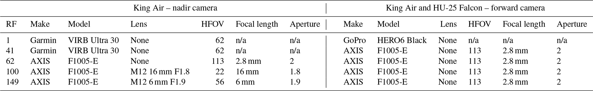
Table 5 summarizes the instrument payload on the HU-25 Falcon, and Table S1 in the Supplement summarizes the instrument performance for each flight. Figure 6 shows the exterior probes and the interior layout of the HU-25 Falcon. As noted earlier, a subset of instruments was not operated in the Winter 2021 deployment (RF48–RF61 from 4 March to 2 April 2021) to accommodate a power issue on the HU-25 Falcon. Those instruments were deemed to be the lowest priority in terms of satisfying the three baseline ACTIVATE objectives summarized in Sect. 2.1.

Table 5 Summary of the HU-25 Falcon instrumentation and measurements. n/a – not applicable.

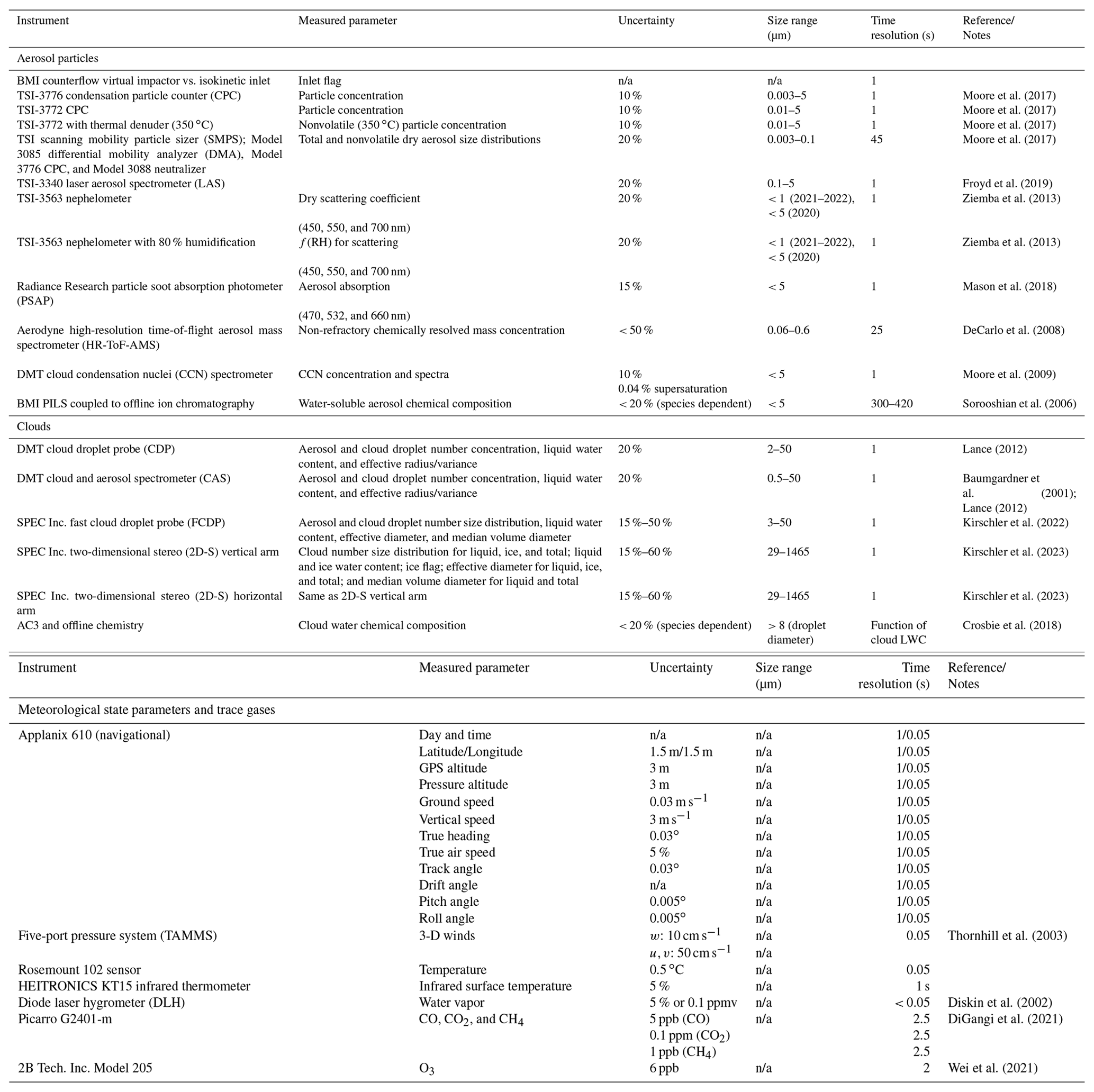
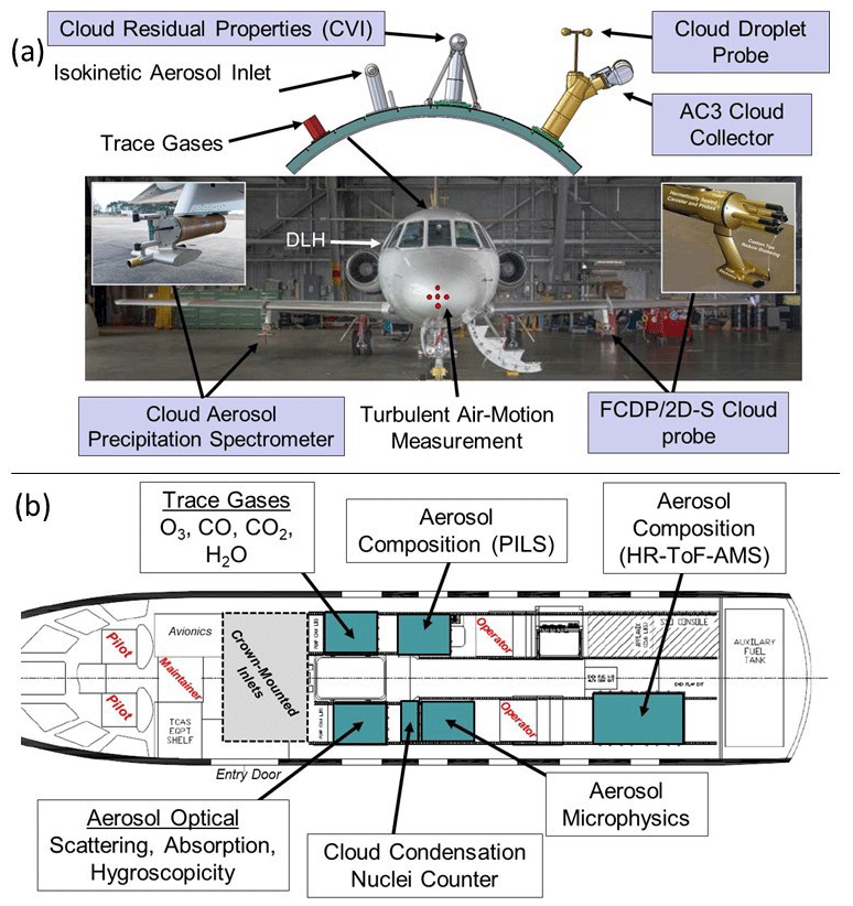
Figure 6 Visual summary of the HU-25 Falcon (a) exterior probes and (b) interior layout. The cloud aerosol and precipitation spectrometer in panel (a) includes the cloud and aerosol spectrometer (CAS) probe described in Sect. 4.5.

4.1 Applanix navigational data

Similar to the King Air, basic navigational and aircraft motion data (calendar day, time, latitude, longitude, GPS altitude, ground speed, vertical speed, true heading, and track, drift, pitch, and roll angle) were obtained with an Applanix 610 system; data were obtained at a native 20 Hz resolution and then averaged to a 1 Hz resolution for archiving. Data at a 20 Hz resolution are available upon request. Similar to the King Air, Applanix data were recorded internally and on the real-time data system and post-processed to obtain increased accuracy and precision via Applanix's proprietary software.

4.2 Diode laser hygrometer and trace gases

Three different instruments were used to measure trace gases including water vapor (H₂O(v)), CO₂, CH₄, CO, and O₃. The diode laser hygrometer (DLH) is an open-path, near-infrared absorption spectrometer (Diskin et al., 2002) that has its optical path entirely outside the HU-25 Falcon cabin, between a window in the cabin and a retroreflector affixed to the instrumentation pylon on the starboard wing. The round-trip beam path was of the order of 8 m with a vertical extent of ∼ 1.5 m and a longitudinal extent of ∼ 2 m, which, coupled with the optical data acquisition rate, define the limit on the temporal and spatial resolution of the measurement. The DLH reported water vapor through 1 and 20 Hz data products, but data are available upon request as fast as 60 Hz depending on airspeed. DLH data are available in clouds, but there was occasional data loss in very dense clouds due to a backscatter artifact. There was also occasional data loss caused by ice formation on the retroreflector, which prevented sufficient optical power from reaching the detector to make a measurement. These data were detected and removed, which reduces the water vapor data available within clouds and during/following icing. In addition to the primary DLH data product, the water vapor mixing ratio, DLH water vapor data are converted to relative humidity with respect to both liquid water and ice using the onboard in situ measurements of ambient pressure and temperature described in Sect. 4.3.

The other two instruments were located entirely within the cabin in a trace gas rack and were extractive, sampling from fuselage-mounted inlets to measure concentrations internally. A Picarro G2401-m measured CO₂, CH₄, and CO at a 0.4 Hz resolution (Digangi et al., 2021) using a modified Rosemount total air temperature probe gas inlet (Buck Research Instruments, LLC) mounted on the crown colocated with the aerosol inlets (Fig. 6a). These measurements were calibrated hourly during flight with a 1 min single-point calibration and weekly during deployments on the ground with a three-point calibration, with all standards traceable to the World Meteorological Organization (WMO) X2019 (CO₂), WMO X2004A (CH₄), and WMO X2014A (CO) scales. Some data from the Picarro were omitted due to inlet leaks, predominantly at high altitude (i.e., RF1–RF9 on 14–27 February 2020). O₃ was measured at 0.5 Hz by a 2B Technologies Inc. O₃ monitor (Model 205), using a forward-facing J-probe inlet mounted on the HU-25 Falcon nadir panel, and relied on a custom sampling apparatus to enhance data quality at high altitude (Wei et al., 2021). O₃ data were zeroed for 1 min with a KI filter every hour during flight to account for baseline drifts and ensure high data quality, and the monitor (Model 305, 2B Technologies Inc.) was calibrated before and after each deployment with a National Institute of Standards and Technology (NIST)-traceable standard. The O₃ data are vulnerable to altitude/pressure dependence that is accounted for based on these routine calibrations, but it is cautioned that there could be residual effects. Interested data users can consult the instrument team regarding these aforementioned effects, and the instrument team contact information is discussed in Sect. 7.

Trace gas mixing ratios can be used in conjunction with back-trajectory analysis to link air masses to source regions, and they can also be used in studies of wet scavenging and aqueous production, as both CO and CH₄ can be considered conserved tracer species. For example, CO and CH₄ are well correlated with a similar relative enhancement ratio for much of the ACTIVATE dataset, consistent with the hypothesis that the observed air was influenced by urban emissions with relative pollutant levels dependent on the degree of dilution. However, there were occasionally periods during which the enhancement factor differed, with CO enhancements much greater than CH₄ in relation to the typical enhancement ratios during the campaign. This is consistent with less efficient forms of combustion, such as biomass burning, with incidences of this observed briefly during several flights near the coast and for longer segments offshore during two flights, RF28 (26 August 2020) and RF38 (23 September 2020). Enhancement ratios of O₃ and CO can also be used effectively to infer chemical information about the air mass. One example is early during the Winter 2022 deployment (January–February) when O₃ and CO were inversely correlated, consistent with NO_x titration of O₃ in a volatile organic compound (VOC)-limited chemistry regime. As the flights moved farther toward spring, this correlation became weaker (March) and then reversed to become a roughly positive correlation between the species (May/June). This is consistent with the switch to an NO_x-limited regime of O₃ photochemistry, as VOC emissions increase with warmer temperatures and the growth of MBL heights, thereby further diluting the anthropogenic NO_x emissions; this highlights another unique advantage of the routine – long-duration measurements of the ACTIVATE dataset.

4.3 Fast-response 3-D winds and state parameters

High-resolution in situ measurements of 3-D winds (u, v, and w components), temperature, and pressure were obtained using the Turbulent Air Motion Measurement System (TAMMS; Thornhill et al., 2003). The system has been installed on the NASA P-3 for over 20 years; however, this was the first time it had been integrated onto the NASA HU-25 Falcon. The raw data were recorded between 100 and 200 Hz with a UEIPAC 300 real-time controller (United Electronics Industries, Inc.) and then averaged down to 20 Hz for archiving and analysis work. Five flush-mounted ports (0.417 cm diameter) were positioned in a cruciform pattern on the nose of the HU-25 Falcon in order to not have any interference in the airflow around the aircraft. The angle of attack was derived from the vertically positioned ports, whereas the sideslip angle was obtained from the horizontally aligned ports. The center tap was a backup for the dynamic (impact) pressure measurement. High-time-resolution and high-precision pressure transducers (Honeywell Precision pressure transducer – next generation, PPT2, and Rosemount) were placed as close as possible to the pressure ports to minimize time delays.

Whereas the five-port pressure system helps determine the speed of the air relative to the aircraft, the speed of the aircraft relative to the Earth was obtained with inertial and GPS data measured via the Applanix 610. Aircraft velocity components are a blended solution using the inertial and GPS data via a Kalman filtering technique (e.g., Brunke et al., 2022). The u and v components are the respective zonal and meridional components, and w is the vertical wind speed (positive is upwards). The 3-D winds are computed using the full version of the well-established air motion equations (Lenschow, 1986).

The total air temperature, from which the ambient air temperature and true airspeed were calculated, was measured by the non-deiced version of the Rosemount Model 102 total air temperature sensor with a fast-response sensing element (E102E4AL, > 5 Hz response). The pressures – total, static, and impact (dynamic) – were obtained with a Rosemount pressure transducer and a Rosemount micro air data transducer (Model 2014MA1A) that was tied into the copilot's pressure port to minimize the pressure defect. An ancillary measurements of the infrared (IR) surface temperature was also included in the TAMMS instrument suite of measurements. IR surface temperature was obtained from a down-looking HEITRONICS KT15 infrared thermometer.

Multiple dedicated calibration flights during each deployment year were performed in order to establish the primary calibration coefficients necessary to ensure the highest data quality. Calibrations were done at different altitudes above the boundary layer in clean homogenous air masses to determine the following parameters:

• angle of attack slope and offset – via speed variations;

• sideslip slope – via crabbing the HU-25 Falcon with wings level;

• pressure defect – via along-wind reverse headings;

• heading offset (sideslip offset) – via cross-wind reverse headings.

These calibration results were then applied to the final data along with any time lag adjustments (Brunke et al., 2022). The Applanix data were also post-processed to reduce the velocity and position errors. The error in positioning for the final data was reduced to less than 1 m. The calibration data were repeatable from year to year and allowed for a final and consistent set of calibration coefficients to be utilized for all the variables except for the heading offset. That value changed between deployments due to the removal and reinstallation of the Applanix on the HU-25 Falcon.

There are several caveats that a potential user should be aware of prior to using these data. For the 3-D winds, users should nominally restrict use to periods during which the HU-25 Falcon is flying straight and level, as significant changes in pitch, roll, and altitude can introduce artifacts and noise into the winds calculation. If non-straight or non-level times are needed for analysis, users are advised to consult the TAMMS instrument team and, at the very least, examine at the data in great detail to look for correlations with pitch or roll that are adversely influencing the derived winds. In addition, care should be taken when averaging the horizontal winds, as the averaging should be done to the u and v components, and the wind speed and direction should then be recomputed post-averaging. When looking at fine-scale details, such as turbulent fluxes via eddy correlation or the average updraft velocity under clouds, users are advised to consider using time windows that overlap by 50 % in order to increase statistics. The time window length should be long enough to capture all of the eddy sizes that contribute to the turbulent fluxes. Assuming the typical ACTIVATE leg length of 3 min and an average airspeed of 100 m s⁻¹, a segment of 512 samples can resolve eddy sizes of up to 1.28 km; thus, if not overlapped, seven full segments can be averaged together to compute the average turbulent fluxes. If the suggested overlap of 50 % is used, 13 full segments can be averaged together to increase statistics significantly.

4.4 Aerosol characterization

In situ measurements of aerosol properties were conducted with the Langley Aerosol Research Group Experiment (LARGE) instrument package used in previous NASA campaigns such as Studies of Emissions and Atmospheric Composition, Clouds and Climate Coupling by Regional Surveys (SEAC⁴RS; Toon et al., 2016) and the Cloud, Aerosol and Monsoon Processes Philippines Experiment (CAMP²Ex; Reid et al., 2023). The majority of aerosol measurements were conducted with instruments integrated inside the fuselage and air provided by two manually switched inlets mounted on the HU-25 Falcon's exterior crown (top of Fig. 6a). An isokinetic Clarke-style shrouded solid double-diffuser inlet (Brechtel Manufacturing Inc. – BMI) was relied on during cloud-free scenes for aerosol characterization (McNaughton et al., 2007), whereas a counterflow virtual impactor (CVI, BMI) was used while in clouds (Shingler et al., 2012) for measurements of droplet residual particles (i.e., particles remaining after droplet evaporation). An inlet flag data product is archived indicating which inlet (i.e., the CVI or the isokinetic inlet) was used at a given time for the high-resolution time-of-flight aerosol mass spectrometer (HR-ToF-AMS) and the laser aerosol spectrometer (LAS) instruments (described below), whereas all other LARGE instruments summarized in this section only sampled downstream of the isokinetic inlet. Those instruments that are not switched to the CVI require in-cloud filtering to remove periods potentially biased by droplet shattering artifacts (discussed in Sect. 4.4.5). The upper-size limit for all bulk observations (unless otherwise noted below) is governed by the isokinetic inlet performance (McNaughton et al., 2007) with a nominal cutoff point at 5 µm diameter (Table 5); it should be noted, however, that this cutoff diameter is for ambient RH conditions, while the final in situ aerosol measurements will be more representative of dried (and thus smaller particle) conditions owing to heating during inlet transmission. All LARGE measurements are archived at a 1 Hz time resolution (unless otherwise noted) and at standard temperature and pressure (STP; 273.15 K and 1013.25 mbar, respectively). The LARGE measurements can be categorized into optical, microphysical, and chemical measurements, which are described in order in the following.

4.4.1 Optical

Dry scattering and absorption coefficients were measured at three wavelengths using a nephelometer (Model 3563, TSI Inc.; 450, 550, and 700 nm; Ziemba et al., 2013) and a particle soot absorption photometer (PSAP; Radiance Research; 470, 532, and 660 nm; Mason et al., 2018), respectively. Scattering coefficient measurements had been corrected for angular truncation (Anderson and Ogren, 1998), and absorption coefficients were corrected using guidance from Virkkula (2010). An aerosol hygroscopic growth factor measurement, f(RH), was calculated in the form of the ratio of total light scattering at high and low RH. Scattering measurements were made by two independent nephelometers in parallel – one at low RH (i.e., generally less than 40 %) and one at high RH (controlled targeting 85 %) – using a custom Nafion humidifier (Ziemba et al., 2013). These measurements allow the calculation of the hygroscopicity gamma parameter, which is then used with the dry scattering coefficient to calculate scattering at any RH up to saturation. The f(RH) data archived are calculated specifically between 20 % and 80 % RH. f(RH) is only reported for conditions when 550 nm scattering coefficients (at both high and low RH) exceeded 5.0 Mm⁻¹ and controlled RH was between 72 % and 92 %.

A 1 µm cyclone was utilized upstream of both nephelometers for 2021–2022 flights; thus, the scattering coefficients and f(RH) represent submicrometer aerosol, in contrast to PSAP data, which represent bulk aerosol. The nephelometer data in 2020 correspond to an upper cutoff point of 5 µm. For the 2021–2022 datasets, we recommend using fast cloud droplet probe (FCDP) microphysical data (which are measured at ambient RH and described in Sect. 4.5) and Mie theory assumptions to calculate ambient extinction for the supermicrometer particle population. The scattering and absorption coefficient data are used to compute secondary properties including scattering and absorption Ångström exponents and single-scattering albedo (SSA), as discussed in Sect. 4.4.4.

4.4.2 Microphysical

Total N_a was measured with two independent condensation particle counters (CPCs). One CPC was sensitive to all particles with a diameter greater than 3 nm (Model 3776, TSI Inc.) and the other only to particles with a diameter greater than 10 nm (Model 3772, TSI Inc.). The difference in number concentration between the two CPCs is informative about ultrafine, and presumably newly formed, particles between 3 and 10 nm for data users interested in research into particle nucleation (Corral et al., 2022b). Nonvolatile particle concentrations (for particles with a diameter greater than 10 nm) were recorded by an additional Model 3772 CPC that was coupled to a 350 ^∘C thermodenuder. The CPC concentrations are useful for assessing the evolution of the full aerosol population, for understanding particles sources and formation processes, and for providing “closure” checks on the integrated size distribution data.

Dry aerosol size distributions are measured by different instruments for varying diameter windows. The ultrafine/Aitken-mode window between 3 and 100 nm diameter is measured with a scanning mobility particle sizer (SMPS; Model 3085 DMA, Model 3776 CPC, and Model 3088 neutralizer; TSI Inc.), which classifies particles based on their electrical mobility diameters. The accumulation-mode diameter window extending from 100 to 5000 nm is captured based on optical diameters using an LAS (Model 3340, TSI Inc.; Froyd et al., 2019). The LAS was calibrated using monodisperse ammonium sulfate particles (i.e., with a refractive index of 1.52) to optimize the relevance to ambient aerosol particles (Shingler et al., 2016), and both sizing instruments were spot-checked frequently to ensure long-term stability using NIST-traceable polystyrene latex spheres at appropriate sizes. Independent empirical size-dependent corrections have been applied to both the SMPS and LAS datasets that allow “stitching” of the distributions at 100 nm; excellent closure is demonstrated for most ambient conditions by adding integrated SMPS and LAS number concentrations compared to total CPC concentrations. A demonstration of this is provided in Fig. 7 for RF12 on 29 February 2020. While the LAS provides 1 Hz data, the SMPS data are at a lower time resolution (∼ 45 s) and require caution with respect to their interpretation when concentrations are rapidly changing during flight. Droplet residual LAS particle size distributions are archived (using the inlet flag) during CVI in-cloud sampling periods. Interpretation of these data has not been demonstrated previously but should provide supplementary information to compositional analysis towards improving our understanding of cloud processing. The LAS–CVI data require the use of the InletFlag (0 denotes isokinetic and 1 denotes CVI) for separation of the two categories of data.

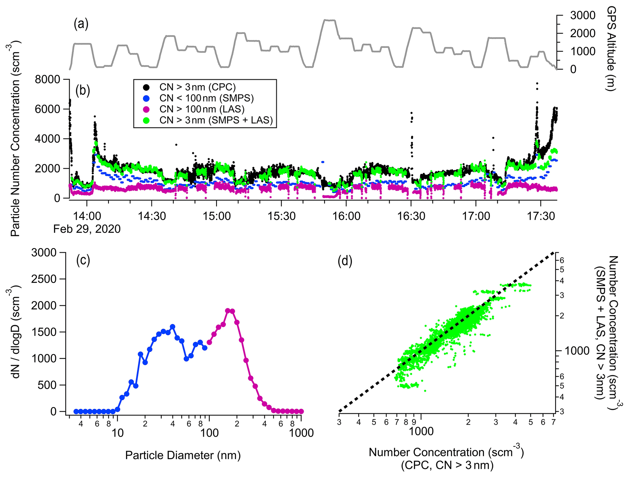
Figure 7 Closure analysis for particle number concentration measurements derived from an ultrafine CPC, SMPS, and LAS. (a–b) Time series data are shown for Research Flight 12 on 29 February 2020, (c) an average size distribution (SMPS in blue and LAS in magenta) during a BCB leg at approximately 16:15 UTC, and (d) a scatterplot of the integrated number concentration derived from LAS and SMPS instruments against the number concentration directly measured by a CPC. Units of “scm⁻³” represent per standard cubic centimeter. In panel (d), orthogonal distance regression (ODR) linear fitting resulted in a slope of 0.961, an intercept of −1.07 cm⁻³, and a coefficient of determination (r²) of 0.868. The mean absolute error (MAE) and mean absolute percentage error (MAPE) values of 148 cm⁻³ and 8.45 %, respectively, are well within the stated uncertainties in Table 5 and demonstrate excellent measurement closure.

Cloud condensation nuclei (CCN) concentrations and spectra for submicrometer particles were measured with a CCN spectrometer (Droplet Measurement Technologies Inc. – DMT) using both constant and scanning flow techniques (Moore and Nenes, 2009). The reported CCN concentration depends on the instrument supersaturation, which is also reported in the data files. For the 2020 dataset, the instrument supersaturation was linearly scanned between approximately 0.2 % and 0.7 % supersaturation with a single upward scan or downward scan consisting of 60 s. For the 2021 and 2022 datasets, the instrument supersaturation was held constant at approximately 0.4 % supersaturation for each flight. Data users are encouraged to consult the data files for the precise, calibrated instrument supersaturation corresponding to each data point.

4.4.3 Chemical

Non-refractory mass concentrations of sulfate, nitrate, ammonium, chloride, organics, and numerous mass spectral markers (mass-to-charge ratio, $m/z$, 42, 43, 44, 55, 57, 58, 60, 79, and 91) were measured by a high-resolution time-of-flight aerosol mass spectrometer (HR-ToF-AMS; Aerodyne; DeCarlo et al., 2008). The nominal vacuum aerodynamic diameter window of the AMS was 60 to 600 nm. As already summarized for ACTIVATE (Dadashazar et al., 2022a), the 1 Hz fast-MS-mode AMS data were averaged to a 30 s time resolution for the data archive. A brief overview of what types of species the aforementioned $m/z$ mass spectral markers represent is as follows: 42 (amines: C₂H₄N⁺), 43 (mixed hydrocarbons: C₃H${}_{\mathrm{7}}^{+}$ or C₂H₃O⁺), 44 (oxidized hydrocarbons: CO${}_{\mathrm{2}}^{+}$), 55 (aliphatic hydrocarbons: C₄H${}_{\mathrm{7}}^{+}$), 57 (aliphatic hydrocarbons: C₄H${}_{\mathrm{9}}^{+}$), 58 (sea salt/marine: NaCl⁺), 60 (biomass burning: C₂H₄O${}_{\mathrm{2}}^{+}$), 79 (methanesulfonate/marine: CH₃SO${}_{\mathrm{2}}^{+}$), and 91 (aromatic hydrocarbons: C₇H₇). The AMS is operated using a custom pressure-controlled inlet (at 500 Torr), and all mass concentrations are reported at STP. The overall AMS ionization efficiency was calibrated using monodisperse 400 nm ammonium nitrate particles throughout the 3-year measurement period, and a collection efficiency value of unity was applied to all data based on comparison to simultaneously measured PILS-based sulfate mass concentrations. AMS–CVI data are reported in separate files (as compared with other AMS data from cloud-free air sampling). The AMS–CVI data include only relative mass fractions. The CVI has been extensively characterized by Shingler et al. (2012), with a demonstration of the utility of AMS–CVI data during ACTIVATE provided by Dadashazar et al. (2022a).

Water-soluble ionic composition was measured by a PILS (BMI) coupled to an offline ion chromatograph (Sorooshian et al., 2006; Crosbie et al., 2020). The time resolution varied between 5 and 7 min depending on the deployment. The PILS data represent bulk aerosol between approximately 50 and 5000 nm. These data include the following anions: chloride, nitrite, bromide, nitrate, sulfate, and oxalate. The following cations are also included: sodium, ammonium, dimethylamine, potassium, magnesium, and calcium. Details of the ion chromatography instrument and the anion and cation speciation analysis methods are provided in recent ACTIVATE studies (Corral et al., 2022a; Gonzalez et al., 2022). The PILS was operated without denuders; thus, users should account for this aspect of the data when interpreting concentrations for semi-volatile species, such as ammonium, for which there may be positive biases due to gas-phase contributions.

4.4.4 Secondary aerosol products

The archived optical and microphysical files are useful starting points for data users interested in summary statistics and special calculated parameters. For example, the optical files include data for submicrometer dry scattering (450, 550, and 700 nm) and calculated extinction (532 nm) coefficients, total aerosol absorption coefficient (470, 532, and 660 nm), f(RH) and its associated gamma parameter at 550 nm, aerosol scattering ($\mathrm{450}/\mathrm{700}$ nm) and absorption ($\mathrm{470}/\mathrm{660}$ nm) Ångström exponents, and the SSA (at 450, 550, and 700 nm). Note that the submicrometer designation applies to 2021–2022 flights and that 2020 flights correspond to bulk aerosol (< 5 µm). The extinction parameter was calculated by summing submicrometer scattering and bulk absorption, with scattering data at 550 nm adjusted to 532 nm using the measured Ångström exponent. As scattering is typically the dominant component of extinction and absorption is assumed to be dominated by brown carbon and black carbon in continental outflow, archived optical properties calculated using a combination of nephelometer and PSAP measurements (i.e., extinction coefficient and SSA) should be treated as representing submicrometer aerosol. Care should be taken with respect to cases suspected to be influenced by absorbing dust, which do not satisfy the assumptions above. The gamma parameter allows one to estimate scattering at any RH (Ziemba et al., 2013); the scattering coefficient, extinction coefficient, scattering Ångström exponent, and SSA are all provided in archived files at ambient RH. Note that ambient scaling assumes that there is no absorption enhancement due to humidification, as we do not have the necessary information regarding the particle mixing state to calculate those enhancements accurately. The microphysical files provide the CPC concentrations along with sub- and supermicrometer number concentration, surface area concentration, and volume concentration from the LAS with the assumption of spherical particles. During data processing, additional filters are applied to the 1 Hz data, such as thresholding and smoothing, to obtain secondary products such as the SSA, which can introduce gaps that do not exist in the raw data. Caution should be taken when averaging ratio-based values such as the SSA, as this can introduce unrealistic values in the data.

4.4.5 Data usage notes

Additional notes on data usage are provided here with the reminder that data users should always also consult with ICARTT data file headers (files described further in Sect. 7) for guidance on data usage. Mass loadings and concentrations are all reported at STP. Conversion factors at a 1 Hz resolution are provided in the ICARTT data files for data users interested in converting the data back to ambient temperature and pressure conditions. The latter step is important for users aiming to compare in situ data to remote-sensing data, as remote sensors retrieve information under ambient conditions.

Aerosol measurements are vulnerable to contamination due to cloud droplet shatter on the sampling inlet when aircraft fly in clouds or precipitation below a cloud; this is usually manifested as unrealistically high particle number concentrations, often with high-frequency variability, as measured by either of the CPCs. It is recommended that data users employ strict criteria and only use aerosol data measured under cloud-free conditions. As an example, a recent ACTIVATE study used aerosol data only when the cloud liquid water content (LWC) was less than 0.001 g m⁻³ (Schlosser et al., 2022). However, users concerned about more confidently separating cloud hydrometeors from coarse aerosol should consult with the instrument teams operating the probes described in Sect. 4.5 and/or develop the types of analyses (e.g., joint histograms) that compare different variables like LWC and N_d to more clearly visualize where clusters emerge for coarse aerosol and how to better separate them from cloud droplets (see Fig. 2 of Schlosser et al., 2022).

As it is a differencing technique, the AMS can produce negative mass concentrations under clean conditions which should be retained in statistical calculations whenever possible. The removal of such points during a level leg, for instance, can positively bias the leg-averaged value.

Owing to the relatively long time resolution of the PILS (5–7 min) and the “smearing” of data without step function responses in composition (Crosbie et al., 2020), data users should use caution with respect to how the data are used for their applications. More specifically, PILS data are unreliable for vertically resolved depictions of ionic composition due to the short amount of time spent during most level legs during ACTIVATE (∼ 3 min) and the fact that spiral and slant profiles were usually shorter than the time needed to collect a PILS sample. In contrast, the data are well suited for statistical assessments of concentrations and chemical ratios relying on the data of many flights, as demonstrated by Hilario et al. (2021).

4.5 Wing-mounted probes (aerosol and cloud droplet size distributions)

Four optical probes were used to characterize aerosol and cloud droplet size distributions extending from 0.5 to 1465 µm. All such data are reported under ambient conditions (temperature, pressure, and RH), which requires caution when trying to compare these aerosol data to the dry aerosol measurements described in Sect. 4.4. A DMT cloud droplet probe (CDP; 2–50 µm) was mounted on the crown of the aircraft fuselage, and a cloud and aerosol spectrometer probe (CAS; 0.5–50 µm) was mounted on the starboard wing (Fig. 6a). Both instruments measure the scattered light pulses as coarse-mode aerosol particles and cloud droplets pass through a laser beam, where the count rate and light intensity are related to the particle number and size, respectively. Particle concentration is computed by multiplying the measured count rate by a sample volume that is the product of the probe sample area and the aircraft true airspeed (TAS). The CDP sample area was experimentally measured by DMT to be 0.323 mm², while an assumed sample area for the CAS of 0.25 mm² was used. In addition, cloud liquid water content (LWC), effective variance, and effective radius were calculated assuming spherical particles with unit density. The CAS is able to measure particles between 0.5 and 2 µm, but its shrouded inlet may make the instrument susceptible to in-cloud droplet shatter, unlike the open-path CDP. The CAS data are archived at 1 Hz, while the CDP data are archived at ≧ 1 Hz depending on the deployment. For 2020, it was observed that 1 Hz data made it hard to distinguish cloud centers and edges, so the data sampling rate was increased for subsequent years of flights.

A fast cloud droplet probe (FCDP; 3–50 µm) and a two-dimensional (2-D) stereo (2D-S; 29–1465 µm), both of which are manufactured by SPEC Inc, were mounted on the port wing (Fig. 6a). The FCDP is a forward-scattering probe with a rapid sampling rate of 25 ns to enable single particle detection for all particles. Its fast electronics and other features, like a small pinhole for coincidence reduction, imply lower uncertainties in particle sizing and counting (Baumgardner et al., 2017; Kirschler et al., 2022; Kleine et al., 2018; Knop et al., 2021; Voigt et al., 2021). Archived FCDP data include aerosol and droplet number size distributions, LWC, effective diameter, and median volume diameter. Extensive processing and corrections to the FCDP data are described in Kirschler et al. (2022). Meanwhile, the CDP and CAS data have not been similarly corrected to date, which may introduce biases, particularly for high-cloud-droplet-number environments exceeding 500 cm⁻³ (Lance, 2012).

The 2-D stereo (2D-S) optical array probe (SPEC Inc.) relies on 128 photodiodes to produce shadow images of single particles (Lawson and Baker, 2006; Lawson et al., 2019). Archived 2D-S data include cloud number size distributions for liquid, ice, and total; liquid and ice water content; ice flag; effective diameter for liquid, ice, and total; and median volume diameter for liquid and total. The 2D-S images are provided upon request, which can be illustrative of hydrometeor shapes (liquid droplets vs. ice) and coarse aerosol types such as bioaerosols. The probe has two identical arms that are perpendicular with 785 nm wavelength lasers associated with each to generate a diffraction pattern for traversing particles. The recorded ensemble of “slices” obtained rapidly by triggered photodiodes helps generate 2-D images of particles (Knollenberg, 1970). The 2D-S used on the HU-25 Falcon has been described in detail by Kirschler et al. (2022), who note that, with the fast response time of 41 ns, the 2D-S has less uncertainty for characterizing spheroids and is in the middle of the range for ice particles compared with other optical array probes (Baker and Lawson, 2006; Gurganus and Lawson, 2018; Lawson and Baker, 2006; Bansmer et al., 2018). For data users interested in stitching together 2D-S size distributions with the other probes like the FCDP, the method discussed by Kirschler et al. (2022) is a suitable option to confront the overlap of the two probes between 16 and 51.3 µm. They did an overlap calculation for the diameter space between the lower FCDP bin bound at 27 µm and the higher 2D-S bin bound at 39.9 µm. Linear interpolation can be applied using the next 2D-S bin and proportionality between the last FCDP bin and the new 2D-S bin. Examples of FCDP and 2D-S data products are shown in Sect. 6 for a representative case flight.

In terms of data usage notes, a few factors should be considered by users:

• It should be kept in mind that the scattered light spectrometers in use are designed for cloud measurements, and uncertainties increase in the case of aerosol measurements. For instance, the sizing for these probes is calibrated assuming water droplets with a corresponding refractive index; thus, if coarse-mode dust, biological particles, and/or sea salt particles are present, there will be sizing biases due to the varying refractive indices and possible aspherical shapes of these aerosol types relative to water droplets.

• The use of the 2D-S horizontal arm is preferable, as the vertical arm did not operate properly in all flights and was disabled in those cases. The data locations are marked accordingly in the vertical arm.

• If the particle size distributions of the FCDP and 2D-S are to be combined, it is recommended not to make the transition above 30 µm, as the measurement area difference in the instruments increases quadratically with size and causes a non-negligible statistical difference, which can manifest itself in unfilled size bins.

• Precipitation particles occur in a considerably lower number than ordinary cloud droplets and, accordingly, the abundance statistics are lower for the 2D-S in this case, which is reflected in an increased measurement uncertainty. This should be accounted for when comparing in situ precipitation measurements with remote-sensing platforms and models.

4.6 Cloud water composition

A special aspect of ACTIVATE was the focus on cloud water measurements due to the extensive amount of time the HU-25 Falcon spent in clouds. Cloud water samples were also collected using the axial cyclone cloud water collector (AC3), which has been characterized and described in detail by Crosbie et al. (2018). The AC3 was mounted on the HU-25 Falcon's exterior crown close to the CVI (top of Fig. 6a). The AC3 extracted cloud water from the airstream when the aircraft was in cloud. A shutter was used at the inlet of the AC3 when the HU-25 Falcon was out of cloud to reduce contamination. Cloud water was collected by vacuum through a Teflon sampling line inside the HU-25 Falcon and deposited in 15 mL high-density polyethylene centrifuge tubes. Samples were stored in a refrigerator post-flight and then analyzed subsequently with ion chromatography (IC), a pH meter, and inductively coupled plasma mass spectrometry (ICP-MS). Owing to the varying liquid volume in each sample vial, the top priority was IC analysis, followed by ICP-MS, and finally pH. The variable volume was due to the different periods of time that the aircraft was in cloud per vial, the varying amounts of cloud LWC during sample collection, and other AC3 performance factors (Crosbie et al., 2018). For context, 70 % (90 %) of the 535 total vials were collected within 6 min (13 min).

The details of the three analytical methods used at the University of Arizona and quality-control details such as collection of sample blanks are described elsewhere for interested readers (Corral et al., 2022a; Gonzalez et al., 2022; Stahl et al., 2021). The IC was able to speciate and quantify the following anions in order of elution: glycolate, acetate, formate, methanesulfonate, pyruvate, glyoxylate, chloride, nitrite, bromide, nitrate, glutarate, adipate, succinate, maleate, sulfate, oxalate, and phthalate. The IC was also able to speciate and quantify the following cations in order of elution: sodium, ammonium, dimethylamine, potassium, magnesium, and calcium. ICP-MS elements detected include the following: Li, Be, B, Na, Mg, Al, S, Cl, K, Ca, Ti, V, Cr, Mn, Fe, Co, Ni, Cu, Zn, Ge, As, Br, Rb, Sr, Y, Zr, Nb, Mo, Ru, Rh, Pd, Ag, Cd, Sn, Sb, Te, I, Cs, Ba, Ce, Hf, Ta, W, Re, Os, Ir, Pt, Au, Hg, Tl, Pb, Th, and U.

Cloud water species concentrations from the IC and ICP-MS are reported in aqueous units (mg L⁻¹), and for conversion to air equivalent units (µg m⁻³) data users can apply their own specific criteria. For context, past ACTIVATE studies have conducted the conversion with knowledge of cloud LWC as derived from the FCDP by using the average LWC during periods of sample collection when the LWC exceeded a threshold of 0.02 g m⁻³ (Corral et al., 2022a; Gonzalez et al., 2022). Aqueous concentrations can be multiplied by the aforementioned mean LWC value during sample collection divided by the density of water. In environments dominated by broken and more vertically developed cumulus clouds, cloud water in edges or tenuous clouds is ineffectively captured. To combat this, Crosbie et al. (2022) used a threshold of 0.1 g m⁻³ and provide a sensitivity analysis for combining cloud water with microphysical data.

4.7 Forward-camera imagery

Depending on the application of HU-25 Falcon data, forward-camera imagery can be critical to visually determine the conditions the aircraft was flying through at a given time. Camera details have already been discussed in Sect. 3.6 and summarized in Table 4. All videos start based on the takeoff times listed in Table 2 and continue until the landing time. However, a significant number of the files end before landing (sometimes up to 15 min) due to the fact that the last file did not close properly once the power was turned off. The files were recorded at a 2 s resolution for 2020 and a 1 s for 2021 and 2022.

4.8 Merge files

Specific to the HU-25 Falcon aircraft are “merge files” on the publicly available data archive (Sect. 7) that are created at different time resolutions of interest (e.g., 1, 5, 10, 15, 30, 60 s, or matching an individual data product's start and stop times). The aim of these files is to accommodate data analysis efforts by synthesizing different time resolutions among instruments in the aircraft payload as well as sampling location. An online merge tool puts different in situ datasets on a common time base using weighted time averages of each dataset. The final archived time base can either be a time series with a constant interval between points or based on an individual dataset's time stamps. The merge tool accounts for data points that have missing or limit-of-detection data codes by skipping over them so as not to bias the resultant values. The merge files have been converted into netCDF (Network Common Data Form) file format (.nc) at 1 and 60 s time resolutions for 2020 (2021 and 2022 forthcoming) in order to be more conducive to modeling and analysis applications by providing more machine-actionable metadata as well as metadata supplied by individual instrument teams. We caution that it is difficult to consider any version of the merge files as “final” due to the potential for instrument principal investigators (PIs) to submit new data sometimes months or even years after flights are completed. However, once new data are submitted, the merge files are typically generated within a month.

5 Complementary data products

5.1 Flight reports

Each individual flight has an archived flight report drafted and reviewed by flight scientists and pilots that can serve as a useful resource for data users aiming to learn more about special features of a particular flight. A caveat is that these reports incorporate notes from scientists and pilots during flight without any post-flight data analysis to provide extra evidence for certain documented features, such as sources of dust or biomass burning. It is recommended that users consult these files and the “Special notes” column of Table 2 to see if relevant details are provided fitting a particular interest, such as instances of mixed-phase clouds, satellite underflights, or air mass types of interest like dust or biomass burning. Of particular importance in the flight reports is the inclusion of flight tracks overlaid on satellite imagery to show cloud conditions.

5.2 HU-25 Falcon flight leg index files

The repeated nature of stairstepping legs flown by the HU-25 Falcon motivated the need for a way to identify leg types as a function of time. This can aid in the analysis of data across multiple flights focused on statistics as a function of leg type. To address this, an individual file was generated per flight day that the HU-25 Falcon flew, identifying 14 different leg types with start and stop times per leg in flight (i.e., a single file contains two flights for double flight days). Within this file, 10-digit indices are provided describing the deployment number, flight number, flight type (process study vs. statistical survey), leg type, ensemble number, and ensemble type (cloud-free or cloudy). The 14 leg types identified include the following (see also Fig. 2): takeoff and landing, transit leg (usually after takeoff and before landing), ACB, BCB, BCT, ACT, MinAlt, Ascent, Descent, Slant/Spiral (i.e., dedicated soundings covering a significant vertical distance beyond what ascents and descents cover during typical stairstepping), BBL, ABL, RS, and Other (any other leg not defined otherwise). It is important to note that leg types are assigned based on the intention of the leg as determined by the flight scientist and are not a description of the data that were collected during that period. For example, an ACB leg could have been flown in a region of scattered cloud above the nominal bases but resulted in no cloud penetrations. Furthermore, process study flights with numerous legs at different levels in cloud may have legs between ACB and BCT called Other (e.g., RF173 on 11 June 2022), and, in some cases, two legs very close to cloud top can be called BCT (e.g., RF13 on 1 March 2020) (Fig. 3b). We caution that, although the usage of these leg files is ideal for analyses depending on large amounts of statistics, it is important to look at as much data as possible to best understand the environmental conditions during a typical leg for more detailed case studies and/or for higher confidence of legs in or out of cloud for a certain percentage of the time of the leg. An example of why this is important is for leg types in the immediate vicinity of clouds owing to the sometimes low cloud fraction and the changing structure of clouds, sometimes including multiple layers of clouds. For applications requiring high confidence in where a plane was relative to clouds, forward-camera videos (Table 4) are very helpful.

5.3 Aircraft collocation product

To address the challenge of geographical and temporal collocation for two separate measurement platforms, a data collocation product (i.e., collocation mask) is available. This product is broadly applicable for any research where data from a secondary platform are required to be within some required spatiotemporal difference with the primary platform. To accommodate different needs, data files are archived when considering either the King Air or the HU-25 Falcon as the primary platform.

Within the contents of each file are the primary platform's 1 Hz time series and colocated secondary-platform time segments along with the corresponding horizontal distance (in km) between each aircraft at each time segment. A colocated time segment is one where the secondary platform is nearest to the primary platform within 15 km and 30 min. If there are multiple separate time segments, it means that there were points where the two platforms flew outside of 15 km and back within the 30 min time segment. Each period was checked, and the nearest colocated time stamp is provided with the corresponding horizontal separation (in km) between the platforms. There are a maximum of 10 colocated segments allowed for each 1 s time step. This product will be described in greater detail in forthcoming work.

5.4 Cloud detection neural network algorithm

Above-aircraft clouds impact the downwelling and upwelling radiation fields by the King Air aircraft and, thus, impact the measurements of airborne passive sensors and their retrieval products, such as the retrieved aerosol and cloud optical and microphysical products. For ACTIVATE, the forward-facing camera on the King Air (Sect. 3.6) was used to create a manual cloud mask product that indicated whether or not a cloud was present above the aircraft. In order to automate this process, the cloud detection neural network (CDNN) algorithm was developed to detect above-aircraft clouds efficiently and automatically using the camera images. The CDNN uses convolutional neural networks to find clouds using forward-viewing camera images. A center-top crop of the forward-facing camera's field of view is used to identify clouds closer (in proximity) to the aircraft. However, this crop may not be fully optimized such that clouds that are too far away to impact passive sensors onboard the aircraft may still be flagged as contaminated by above-aircraft clouds. Moreover, clouds that are not directly visible in the forward-facing camera, such as above-aircraft clouds behind the aircraft that are nonetheless blocking the sun, are unable to be detected. The description of the CDNN, its performance, and the resulting archived ACTIVATE cloud mask product results are detailed in Nied et al. (2023).

5.5 MERRA-2 data along flight tracks

The Modern-Era Retrospective analysis for Research and Applications, version 2 (MERRA-2) (Gelaro et al., 2017) is NASA's latest reanalysis generated with the Goddard Earth Observing System, version 5 (GEOS-5) atmospheric data assimilation system (Rienecker, 2008). It has a 0.5^∘ × 0.625^∘ horizontal resolution with 72 vertical levels from the surface to 0.01 hPa. Its aerosol reanalysis (Buchard et al., 2017; Randles et al., 2017) uses the GEOS-5 Goddard Aerosol Assimilation System (Buchard et al., 2015), which utilizes the Goddard Chemistry, Aerosol, Radiation, and Transport model (GOCART) (Chin et al., 2002) to simulate 15 externally mixed aerosol tracers: hydrophobic and hydrophilic black carbon (BC) and organic carbon (OC), dust (five size bins), sea salt (five size bins), and sulfate. GOCART includes wind-speed-dependent emissions for dust and sea salt, fossil fuel combustion, biomass burning and biofuel emissions for primary sulfate and carbonaceous aerosols, and additional biogenic sources for organic carbon. Secondary sulfate is formed by chemical oxidation of SO₂ and dimethylsulfide (DMS). Volcanic SO₂ emissions are included. The major sinks for aerosol particles are gravitational settling, dry deposition, and wet removal due to stratiform and convective precipitation. MERRA-2 assimilates the aerosol optical depth (AOD) from ground- and satellite-based remote-sensing sensors, including the Advanced Very High Resolution Radiometer (AVHRR), the Aerosol Robotic Network (AERONET), the Multi-angle Imaging Spectroradiometer (MISR), and the Moderate Resolution Imaging Spectroradiometer (MODIS/Terra and MODIS/Aqua). MERRA-2 aerosol data have been evaluated by Randles et al. (2017) for AODs and by Buchard et al. (2017) for aerosol vertical distribution and absorption.

We have archived a data product that samples MERRA-2 for selected 3-D fields along the HU-25 Falcon flight tracks during the ACTIVATE deployments (Table 6). We interpolate the original MERRA-2 3 h instantaneous 3-D fields to the latitude, longitude, and pressure altitude of the aircraft every 60 s along the flight track. Data files for February–March and August–September 2020 are archived, and the product files for subsequent years are being generated for archiving at the same location (details of accessibility given in Sect. 7). These sampled MERRA-2 data facilitate the comparison between aircraft measurements and reanalysis and provide quantities that are not measured during ACTIVATE (such as the SO₂ concentration; Corral et al., 2022b). They are also useful for undertaking statistical analysis of aircraft in situ data in comparison with reanalysis as well as model evaluation.

Table 6 MERRA-2 data fields sampled along the HU-25 Falcon flight tracks during ACTIVATE (see Sect. 5.5). STP represents standard temperature (0 ^∘C) and pressure (1013.25 hPa).

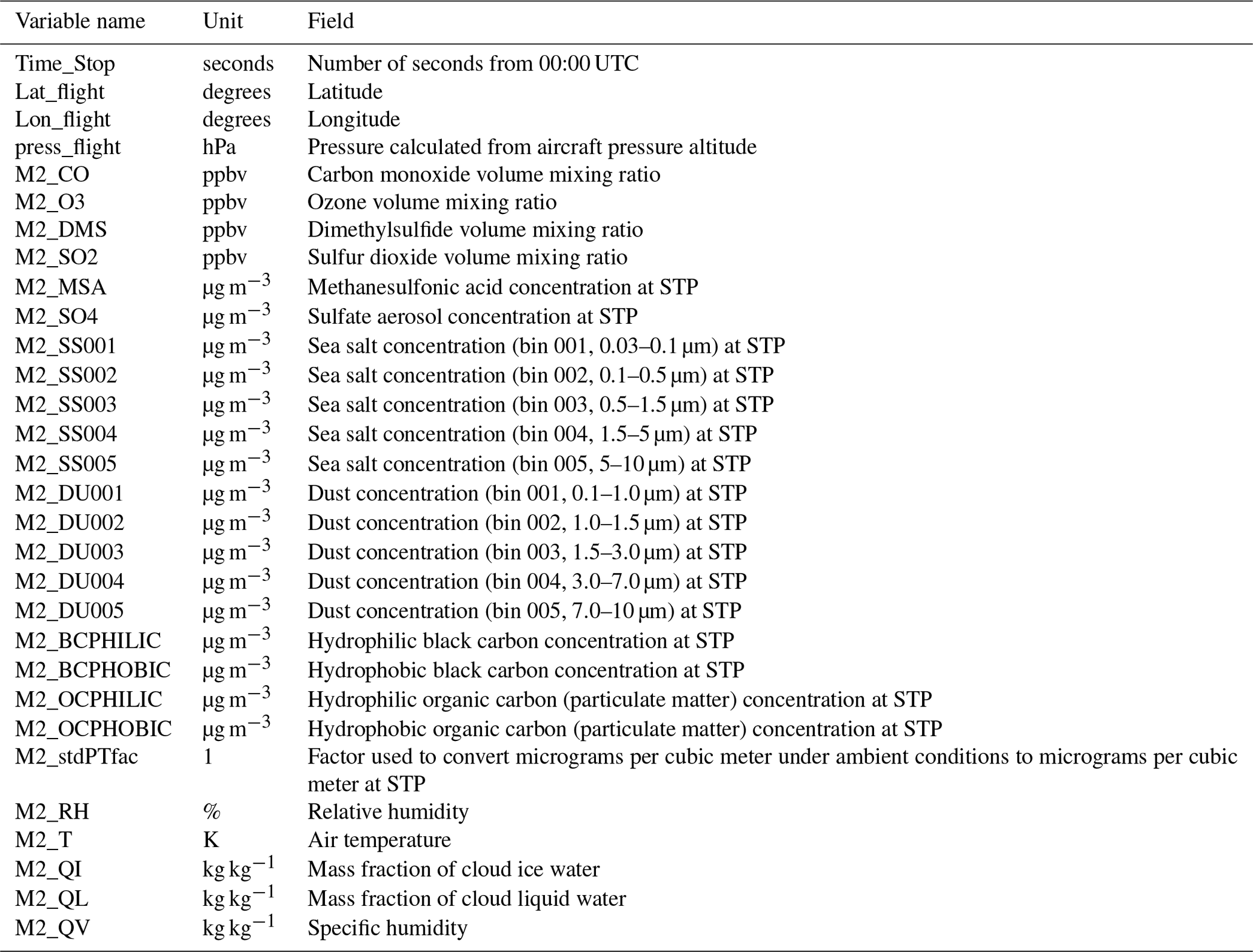
5.6 FLEXPART back-trajectory products

The Lagrangian transport and dispersion model, FLEXPART (FLEXible PARTicle dispersion model, https://www.flexpart.eu/, last access: 1 May 2023; Pisso et al., 2019; Eckhardt, 2008), is used to simulate transport pathways of air masses associated with ACTIVATE aircraft measurements. In its backward mode, FLEXPART calculates trajectories of a multitude of particles and simulates advection, convection, and turbulent dispersion of the particles during the transport period. Detailed descriptions of the FLEXPART transport schemes and parameterizations can be found in the literature (Eckhardt, 2008; Zhang et al., 2014). All FLEXPART simulations were driven by the Global Forecast System Analysis (GFS-ANL 003, 1^∘ × 1^∘, 26 levels, 3 hourly; https://www.ncei.noaa.gov/data/global-forecast-system/access/grid-003-1.0-degree/analysis, last access: 1 May 2023). FLEXPART version 9.2 was used for the ACTIVATE February–March and August–September 2020 deployments. For the 2021 and 2022 campaigns, FLEXPART v10.4 (Pisso et al., 2019) was used to accommodate the recent upgrade in the GFS-ANL data as well as to gain a better capacity with respect to simulating turbulence in the boundary layer. The purpose of this simulation series is to depict general transport pathways from a large-scale perspective. Model configurations here (e.g., output frequency and boundary layer turbulence) are not prioritized for small-scale analysis. The FLEXPART trajectory products for both the 2020 and 2021 campaigns are now available to assist with the analyses of aerosol sources and aging history associated with aircraft measurements; 2022 files are forthcoming.

In the FLEXPART backward mode, a plume of passive particles is released from the aircraft location and advected and dispersed backwards in time. For each 60 s merged aircraft measurement, FLEXPART initiates 10 000 passive particles at the sampling location every 10 min and calculates backwards for 10 d. The released particles represent the air masses (plume) intercepted by the aircraft. For a completed backward simulation, the total residence time (RT) of the plume in a given 1^∘ × 1^∘ grid cell can be calculated by summing the time duration of all particles that were present in the cell during the 10 d transport period. If a large fraction of particles passes through a surface grid cell multiple times, the grid cell would accumulate a long RT, and emissions therein would have a large contribution to the plume intercepted by the aircraft. The horizontal distribution of vertically integrated RTs (Fig. 8a) can be readily used to determine a trajectory-like transport pathway, while the vertical distribution of the RT (Fig. 8b) can clearly indicate the plume transport height and the acquisition of surface emissions.

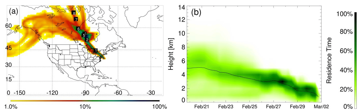
Figure 8 (a) Horizontal and (b) vertical views of the simulated air mass residence time (RT) for flight measurements at 19:22 UTC on 1 March 2020 (RF14). The labels with the white numbers on the map in panel (a) indicate the locations of the maximal RT for the corresponding upwind day. Transport pathways differ significantly, and the absolute RT values may vary a lot between cases. For a better comparison of transport pathways between cases, the RT is expressed as a percentage of the maximal integrated value during the 10 d trajectory period. The RT is color-coded using (a) logarithmic and (b) linear scales, respectively.

For each of the six ACTIVATE deployment periods, two types of files can be found in the ACTIVATE data. One type includes trajectory plots associated with the aircraft data for every 10 min. For each trajectory, a map plot and a vertical plot of the RT distributions are included. Examples are shown in Fig. 8 for aircraft measurements at 19:22 UTC during the second flight on 1 March 2020, which is also discussed in more detail in Sect. 6. These plots are generated for quick-look purposes in order to visualize transport pathways; thus, the plot quality is constrained to limit total file size. The other file type includes original FLEXPART output for 10 d backward trajectories released every 10 min along flight tracks. Each netCDF file contains the gridded specific residence time (RT, in s m³ kg⁻¹) of all released particles. The RT is saved in such a unit instead for time (in s) so that it can be easily multiplied by any upwind source or emission (in kg m⁻³ s⁻¹) to calculate source contributions affecting the receptor point. For example, the FLEXPART RT can be used to calculate a time series of tracer concentrations at the receptor contributed by a certain emission source (e.g., anthropogenic or biomass burning) by multiplying the residence time in the lowest 300 m by the emission flux.

Uncertainties in transport pathways simulated by FLEXPART can be due to the parameterizations representing temporally and spatially unresolved transport processes (Stohl et al., 2005). In terms of vertical transport processes, boundary layer mixing and convective updrafts are both treated in FLEXPART using information from the driving meteorology. Time-varying planetary boundary layer (PBL) height determines the vertical mixing of air parcels. In FLEXPART, the PBL height is calculated using the Richardson number concept based on the wind and temperature fields (Vogelezang and Holtslag, 1996). Another highly parameterized sub-grid process is cloud convection. FLEXPART redistributes air parcels vertically in convection-activated grids using the approach of Emanuel and Živkoviæ-Rothman (1999), which determines air parcel displacement in up- and down-drafts based on temperature and humidity fields. Model results with such schemes have been tested and validated using surface and in situ measurements (Brioude et al., 2013; Stohl et al., 1998).

5.7 MODIS, GOES-16, and MERRA-2

To assist data analysis efforts for ACTIVATE that can benefit from contextual satellite and reanalysis data for overlapping and prior time periods, various satellite and reanalysis data products are archived with a common format and spatial resolution. The dataset is comprised of products generated at two spatial resolutions: 1^∘ × 1^∘ and 2 km (satellite pixel resolution). The 1^∘ × 1^∘ data correspond to aerosol and cloud properties derived from MODIS Aqua (Level-3 product), paired with MERRA-2 meteorological parameters regridded to the same resolution. Satellite pixel-level cloud properties are from the Advanced Baseline Imager (ABI) on the 16th Geostationary Operational Environmental Satellite (GOES-16), with continuous spatiotemporal sampling of the ACTIVATE domain. While the Level-3 products are intended for understanding the large-scale and climatological features of the study region, the pixel-level GOES-16 retrievals are valuable for monitoring the spatiotemporal evolution of the cloud fields during research flights. Merged satellite–reanalysis daily files combine 3-D meteorological fields from MERRA-2 (already described in Sect. 5.5) with daytime aerosol and cloud properties derived from MODIS on Aqua (∼ 13:30 local solar time overpass time) for the January 2009–July 2022 period and the domain defined by the 10.5–59.5^∘ N, 84.5–30.5^∘ W box. MODIS cloud retrievals are taken from the Cloud and the Earth's Radiant Energy System (CERES) Edition 4 (Minnis et al., 2021) Level-3 Single Scanner Footprint (SSF1deg-Day), gridded at a 1^∘ × 1^∘ resolution. CERES–MODIS cloud properties in the merged file are cloud amount, cloud effective pressure, cloud effective temperature, cloud effective height, cloud particle effective radius (ice and liquid) derived using the 3.7 µm channel, water path (ice and liquid), cloud optical depth, and liquid cloud droplet number concentration estimated following Painemal (2018). MODIS AODs (Levy et al., 2013) at a 1^∘ × 1^∘ resolution for seven wavelengths (0.47, 0.55, 0.66, 0.86, 1.24, 1.63, and 2.13 µm) are obtained from the MODIS Level-3 Atmospheric Gridded Product Collection 6 (MYD08_D3). Examples of ACTIVATE applications of this dataset include climatological characterization of the atmospheric circulation and cloud field (Painemal et al., 2021), assessment of the meteorological factors that modulate clouds and aerosol variability and their implications for aerosol–cloud interactions (Dadashazar et al., 2021b), and description of the synoptic-scale processes that give rise to boundary layer cloud variability (Painemal et al., 2023).

MERRA-2 meteorological parameters at a 0.625^∘ × 0.5^∘ resolution are spatially colocated with MODIS via nearest-neighbor interpolation. We selected MERRA-2 products at 18:00 UTC, as it is the closest match to the Aqua overpass time for the northwest Atlantic. In addition, 15 isobaric levels are stored, corresponding to (units of hPa) 1000, 975, 950, 925, 900, 875, 850, 825, 800, 775, 750, 725, 700, 650, and 600. MERRA-2 3-D fields (longitude × latitude × vertical level) include air temperature, RH, sea level pressure, edge heights, eastward wind, northward wind, and vertical pressure velocity, whereas 2-D fields (at a fixed vertical level) are surface skin temperature, 2 m eastward wind, 2 m northward wind, and lifting condensation level.

GOES-16 ABI cloud retrievals are derived using the NASA Satellite ClOud and Radiation Property retrieval System (SatCORPS) algorithms (Minnis et al., 2008, 2021). SatCORPS algorithms have been adapted from those for CERES–MODIS in order to take advantage of radiometric channels similar to those of MODIS and other Earth-orbiting satellites (Minnis et al., 2021). Additional consistency between MODIS and GOES-16 is achieved by calibrating GOES-16 visible radiance against its MODIS Aqua counterpart, following Doelling et al. (2018). GOES-16 cloud retrievals are produced every 20 min during the ACTIVATE deployment. Files are archived for two regions covering the ACTIVATE flight tracks: a small domain (29–46^∘ N, 78–60^∘ W), and a large domain (18–55^∘ N, 93–49^∘ W). Cloud properties for the small domain are produced at the native resolution of the infrared channels – that is, 2 km at nadir. For the large domain, 2 km cloud properties are subsampled every other pixel to achieve a spatial resolution of 4 km. Cloud products derived from GOES-16 include cloud mask and phase, temperature, height and pressure, particle effective radius (ice and liquid), water path (ice and liquid), and optical depth. The ability of GOES-16 products to resolve the diurnal cycle at a relatively high spatial resolution makes the retrievals particularly useful for describing the evolution of the cloud fields during the research flights (GOES-16 snapshots are included in the flight reports described in Sect. 5.1). GOES-16 products have been used in the context of ACTIVATE for validating mesoscale simulations of clouds (Chen et al., 2022), for assessing the evolution of the liquid water path in large-eddy simulation (LES) experiments (Li et al., 2022), and for quantifying the cloud-top entrainment rate and its role in the CCN budget (Tornow et al., 2022). In addition, GOES-16 retrievals are well suited for matching with the aircraft tracks to complement in situ observations as well as for Lagrangian studies.

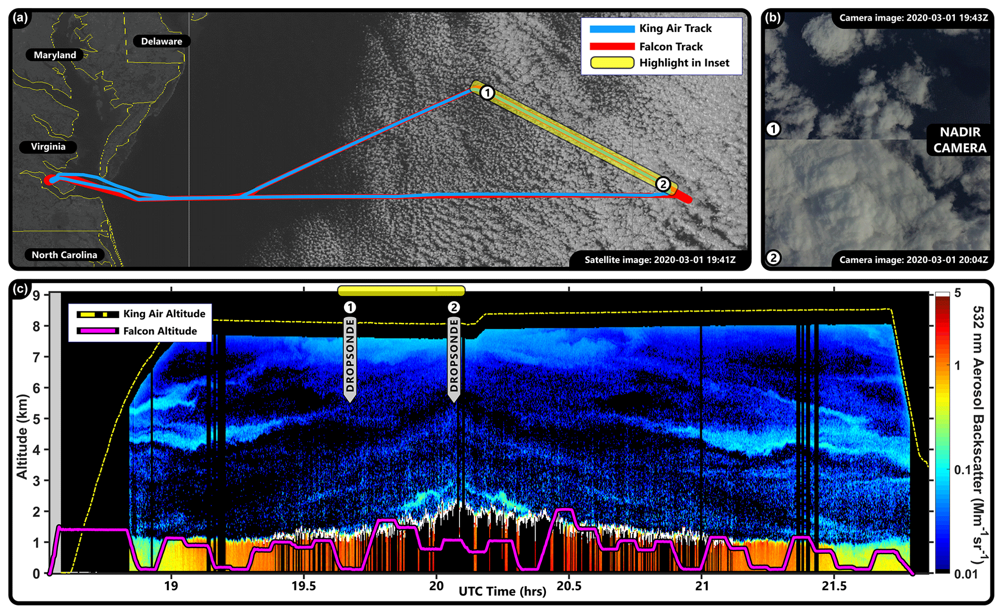
Figure 9 (a) Flight tracks of the King Air and HU-25 Falcon for RF14 on 1 March 2020 overlaid on GOES-16 visible imagery captured at 19:41 UTC. The number 1 and 2 labels correspond to where the two respective dropsondes were launched along the downwind leg (highlighted in yellow) during this flight. These indicators are consistent in all three panels. Panel (b) shows nadir camera imagery from the King Air at the time the two respective dropsondes were launched. Panel (c) presents time series of the King Air aerosol backscatter shown as curtain profiles, along with the altitude trace of the King Air and HU-25 Falcon aircraft; shown also are the locations where the two respective dropsondes were launched, and the downwind leg is highlighted in yellow.

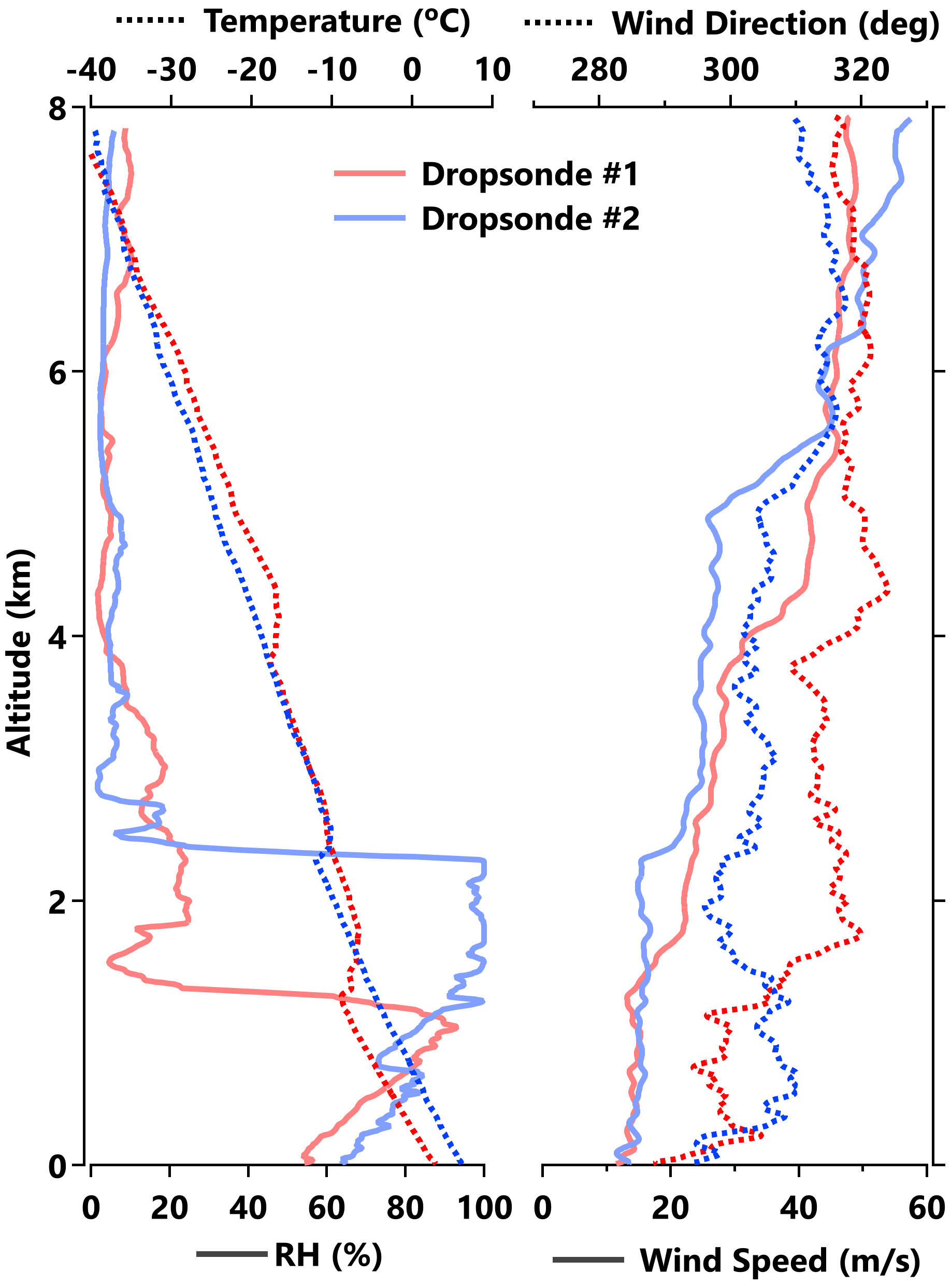
Figure 10 Vertical profiles of variables measured with the two dropsondes launched during RF14 (1 March 2020); the drop locations are shown in Fig. 9.

6 Case flight example

The afternoon joint flight on 1 March 2020 is highly representative of the majority of the ACTIVATE flight dataset in terms of how the aircraft flew and the science that was targeted. This section aims to share representative data collected to summarize how the aforementioned data products in Sects. 3–5 can be visualized and used; this day of flights was also summarized during an open-data workshop that was recorded and has been archived at https://asdc.larc.nasa.gov/news/activate-data-webinar-materials (last access: 1 May 2023). While this flight was a canonical type of ACTIVATE flight due to it being a statistical survey, the actual conditions presented qualified this day as an excellent flight day, as anticipated based on the weather forecasting meeting on the previous day. This is because of forecasted cold-air outbreak (CAO) indicators of boundary layer instability (Papritz et al., 2015; Painemal et al., 2021; Fletcher et al., 2016) coinciding with strong, cold, northwesterly winds and “cloud streets” (Dadashazar et al., 2021b). The day was also forecasted to have a high cloud fraction and no high-level cirrus or mid-tropospheric cloud layers that would negatively impact remote-sensing objectives. Forecasting analysis conducted the previous day suggested that there would be a broken-to-overcast low cloud deck (deepening to the east) with a western edge moving farther offshore throughout the day. GEOS forward processing data hinted at a fairly low aerosol loading, with increasing sea salt concentrations offshore. Actual conditions were consistent with the forecasted information.

The first joint flight on 1 March 2020 was a process study flight (Fig. 3a), as the aircraft transited to an area of high interest and conducted maneuvers deviating from the ensemble approach shown in Fig. 2. More specifically, the HU-25 Falcon conducted stacked level legs (a wall) approximately perpendicular to the estimated boundary layer winds while the King Air flew a large circle encompassing the wall location followed by an overpass of the extended axis of the HU-25 Falcon wall. This particular flight has also been simulated and discussed in recent studies (Chen et al., 2022; Li et al., 2022; Tornow et al., 2022). Both aircraft returned to the base of operations (Newport News) to refuel and then returned to the same region as in the morning, flying a downwind survey that started at the wall center point and extended as far as fuel permitted (Fig. 9a). The downwind survey leg allowed for a semi-Lagrangian characterization of the air mass evolution and also resampled the air mass from the morning flight. Both flights captured elements of the cloud morphology common to CAOs, but the afternoon flight characterized the evolution from the upwind clear region to scattered cumulus transforming into a thicker and more extensive layer before finally transitioning into an open-cellular stratocumulus organization. This can be seen from flight tracks overlaid on GOES-16 visible imagery (Fig. 9a).

FLEXPART simulation results pertaining to air mass trajectories arriving at the point of the HU-25 Falcon during this flight at 19:22 UTC are shown in Fig. 8. Figure 10 shows the level of detail possible with dropsondes, Fig. 9a presents the markings of where the two respective dropsondes were launched, and Fig. 9b gives the nadir camera imagery from the King Air at those times. Representative data from the HSRL-2 in the form of vertical “curtains” of aerosol backscatter as a function of flight time are shown in Fig. 9c; these data show that higher aerosol loading is located in the MBL closest to the ocean surface. This panel also shows the altitude of the HU-25 Falcon while flying below the King Air aircraft as well as the locations where the respective dropsondes were launched from the King Air.

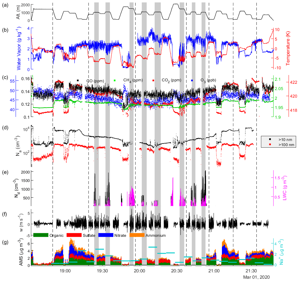
Figure 11 Time series (UTC time) of HU-25 Falcon data for RF14 on 1 March 2020. Shown are the archived HU-25 Falcon in situ data for (a) altitude (Applanix 610), (b) water vapor (DLH) and temperature (Rosemount 102 sensor), (c) trace gases (Picarro G2401-m for CO, CO₂, and CH₄; 2B Tech. Inc. Model 205 for O₃), (d) aerosol particle number concentration for diameters > 10 nm (TSI-3772 CPC) and > 100 nm (LAS), (e) cloud droplet number concentration and LWC (FCDP), (f) vertical wind speed (TAMMS), and (g) speciated aerosol mass concentrations from the AMS (organic, sulfate, nitrate, and ammonium) and PILS (sodium). Shaded gray vertical sections denote the two level-leg types in cloud (above cloud base, ACB, and below cloud top, BCT). The dashed vertical black bars mark the beginning of either clear or cloudy ensembles (ensembles in order: clear, cloudy, cloudy, cloudy, clear, and clear).

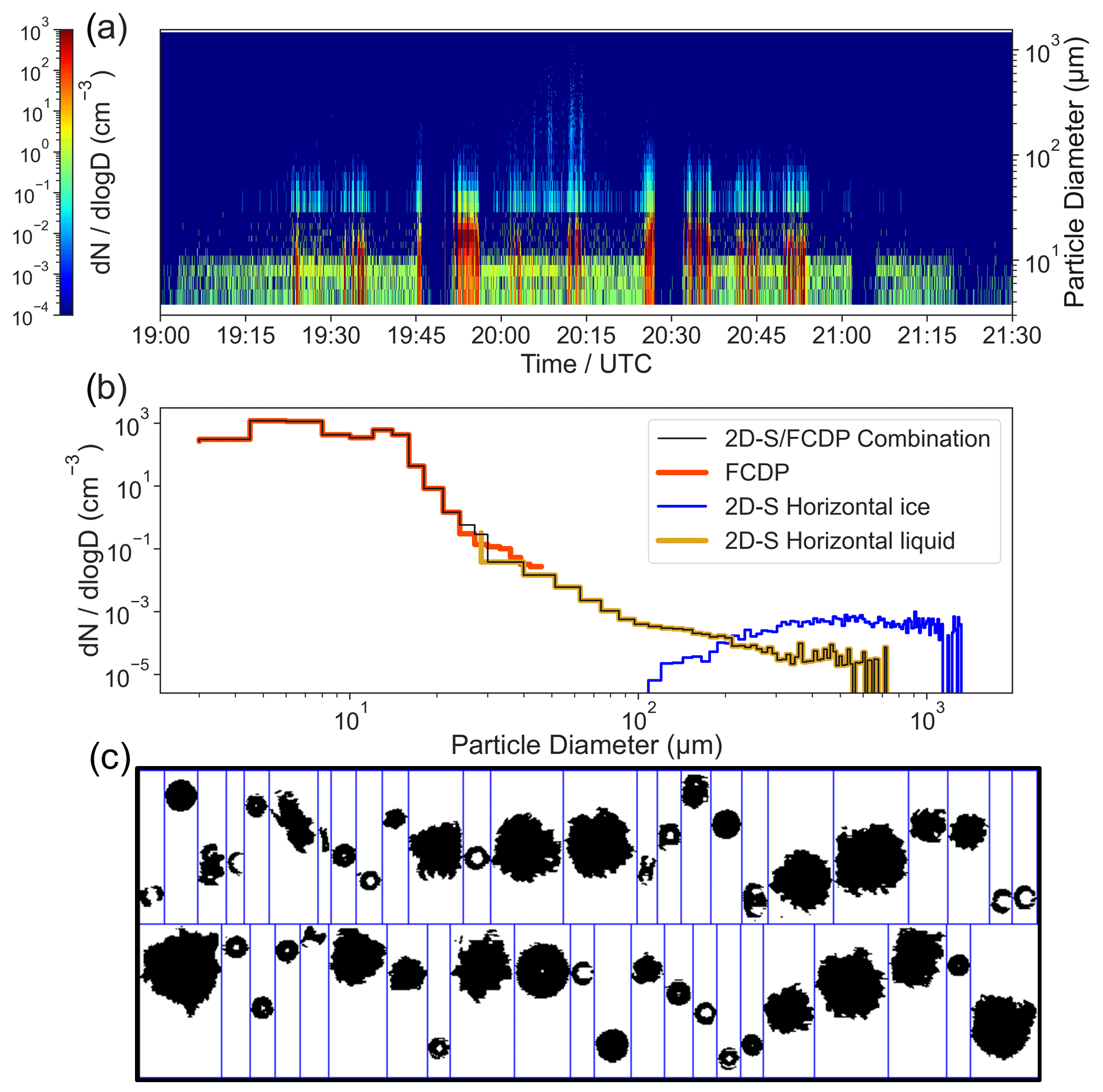
Figure 12 Representative data products derived from the FCDP and 2D-S instruments on the HU-25 Falcon for RF14 on 1 March 2020: (a) time series of cloud droplet size distribution based on combining FCDP and 2D-S data, (b) average size distribution of liquid (FCDP and 2D-S horizontal) and ice (2D-S horizontal) for cloud measurements with LWC > 0.02 g m⁻³ and N_d > 10 cm⁻³, and (c) example images captured by the 2D-S horizontal probe for 20:05:35–20:05:50 UTC.

Table 7 Summary of where to access the different datasets and resources described in this paper. n/a – not applicable.

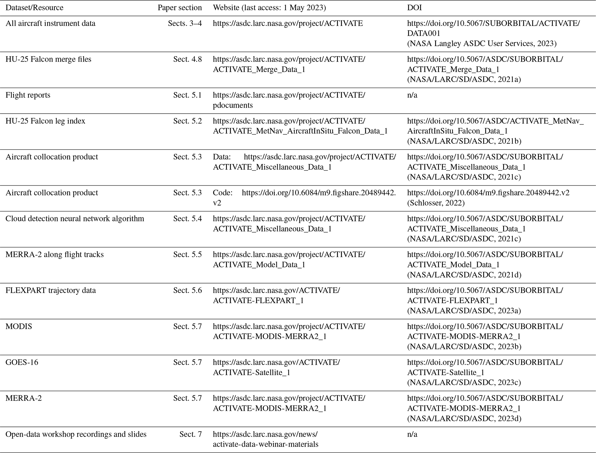
Figure 11 summarizes selected variables measured by the HU-25 Falcon in time series format. The dashed vertical black bars denote the beginning of either clear or cloud ensembles. The first ensemble begins right after the high-altitude transit following takeoff and was a clear ensemble with the following legs in order: MinAlt, ABL, BBL, RS, and MinAlt. That ensemble was followed by three consecutive cloud ensembles, with the first two containing the nominal order of legs described in Sect. 2.2 while the third ensemble was truncated at MinAlt owing to the absence of clouds, which is clearly visible in Fig. 9a with clear conditions closer to the coast. The vertical gray shaded bars make use of leg index files (Sect. 5.2) and distinguish the two level-leg types in cloud. including ACB (above cloud base) and BCT (below cloud top). Clearly, those periods are marked by enhancements in N_d and LWC as measured by the FCDP, but the reader should note that cloud penetrations also occur outside of designated cloud legs, such as during altitude transitions. Many of the other plotted variables associated with trace gases, aerosol particles, temperature, and wind data show an interesting structure that, at least partly, is dependent on aircraft altitude, which can be teased out in these forms of multi-panel time series depictions (as in Fig. 11) that can aid data users. Aerosol microphysical data have been screened to remove data collected in clouds and, in the case of the LAS (which was used to determine number concentration above 100 nm), using the inlet flag variable to remove CVI data from this illustration. Note that AMS data are archived separately for isokinetic and CVI time periods, so this screening is not necessary for the AMS. An important note with respect to the aerosol composition data is that the PILS data for Na⁺, used here as a proxy for sea salt that the AMS cannot provide, have a coarser time resolution than the AMS data. Furthermore, some PILS data may potentially include an influence from cloud periods and, thus, may not be suitable for certain applications. If data users want aerosol data without any cloud contamination, they should only use PILS data in cloud-free areas, such as clear ensembles and transit periods. For interested readers, a figure analogous to Fig. 7 is also shown in Fig. S1 in the Supplement for this flight case in order to demonstrate again how to conduct closure types of analyses between different data parameters, such as aerosol number concentration in this case.

Lastly, Fig. 12 provides a summary of cloud probe products specifically from the FCDP–2D-S combination probe from the HU-25 Falcon's port wing. Figure 12a shows a time series of cloud droplet size distributions from the FCDP combined with the 2D-S. Sections with cloud penetrations are clearly visible, with enhanced number concentrations above 10 µm. Also evident from the time series are periods with noticeable number concentrations below 10 µm during periods without clouds, which is indicative of coarse aerosol particles such as sea salt. Figure 12b shows various forms of size distributions that data users can produce from FCDP alone, in addition to the 2D-S–FCDP combination and 2D-S horizontal ice and liquid products. The stitched size distribution for 2D-S–FCDP is explained briefly in Sect. 4.5 and has been described more extensively by Kirschler et al. (2022). The 2D-S imagery in Fig. 12c covers a 20 s period that nicely represents a broad variety of large particle shapes, including liquid droplets and rimed ice particles.

7 Code and data availability

NASA's Atmospheric Science Data Center (ASDC) plays a key role in the data curation, dissemination, and long-term preservation of ACTIVATE data. It archives the latest versions of publication-quality data, including observational, derived, and value-added data products. It also houses contextual information to facilitate data use by the research community at large, in addition to documentation for maintaining reprocessing capability and openness. Digital object identifiers (DOIs) are assigned at both the project level and data product (collection) level for ACTIVATE. All data from the King Air and HU-25 Falcon, including the complementary data products from Sect. 5, unless otherwise stated, are publicly archived on ASDC's Distributed Active Archive Center (DAAC; https://doi.org/10.5067/SUBORBITAL/ACTIVATE/DATA001, ACTIVATE Science Team, 2020) and are accessible via the ACTIVATE landing page (https://asdc.larc.nasa.gov/project/ACTIVATE, last access: 1 May 2023), with each data file containing data from one flight or 1 calendar day. Various tabs on that web page include different data products (collections) and their unique DOI codes, which are summarized in Table 7 along with other resources described in this paper. The open-data workshop content listed in Table 7 is especially important to guide new data users through each step of the process to access and visualize data, beginning with the establishment of a free account at https://earthdata.nasa.gov (NASA, 2023a) and then proceeding to download ACTIVATE data with the Sub-Orbital Order Tool (SOOT; https://asdc.larc.nasa.gov/soot/power-user, NASA, 2023b). ACTIVATE data are also available to download via Earthdata Search: https://search.earthdata.nasa.gov/search?fpj=ACTIVATE (NASA, 2023c).

Most files are in a special format called ICARTT (Northup et al., 2017), which is traditionally used by NASA and other agencies for airborne data. HU-25 Falcon in situ observations are reported in ICARTT format, whereas remote-sensing data uses a combination of the ICARTT format and hierarchical data format (HDF). It is critical for any data user aiming to use airborne science data to review the ICARTT file headers that provide guidance on how to both use and interpret data from individual instruments.

File names constitute the following details in order: campaign, instrument, sampling method, start date, revision number, and the (optional) end date. Publication-quality data include a revision number in their file name (R0+) and are time synced to the platform time standard (DLH instrument time for HU-25 Falcon and GPS time for King Air). The contents of each ICARTT file include data notes in a README tab, including contact information for the instrument data (i.e., instrument PI name and data manager – DM), PI institution, campaign name, start date of data collection, most recent data revision date, number of variables, data flags, instrument details and description of the data, and revision log. The revision log lists the identifier of the current data revision as well as the previous revisions and their relative status. Each instrument will have its own unique column headers based on what was being measured.

While the instrument teams have time synchronized the datasets with one another to account for different sampling techniques (e.g., varying times for sample air to travel from an inlet to instruments), it is possible that variation of a few seconds can occur. No post-submission time alignment is done by the data management team, merge process, or ASDC DAAC; thus, data users should use diligence when utilizing multiple datasets to carry out intercomparisons and should also confirm that temporal variations in related parameters match one another without obvious systematic shifts.

8 Conclusions

A collection of airborne datasets is introduced here that serves as a resource for investigations of aerosol–cloud–meteorology interactions, along with studies more interested in measurements of just trace gases, aerosol particles, clouds, precipitation, and/or atmospheric state parameters. The datasets cover the northwest Atlantic, extending from the coastal area of the mid-Atlantic states and New England to much farther offshore around the vicinity of Bermuda where more remote marine conditions are present that are less perturbed by continental emissions. The data span all seasons, with collection periods between November–June and August–September for 2020 through 2022. This paper is a potential user's guide to the access and availability of ACTIVATE data products. Of particular interest to most data users of the HU-25 Falcon data is likely the merged dataset of variables generated at different time resolutions of interest (e.g., 1, 5, 10, 15, 30, 60 s, or matching an individual data product's start and stop times). Data products and codes have also been developed to help users with the joint analysis of data between the two aircraft based on specific criteria of interest related to time and space separation.

Appendix A: Summary of abbreviations

Abbreviation	Definition
2D-S	Two-dimensional (2-D) stereo
ABI	Advanced Baseline Imager
ABL	Above boundary layer top
AC3	Axial cyclone cloud water collector
ACB	Above cloud base
ACE-ENA	Aerosol and Cloud Experiments in the Eastern North Atlantic
ACT	Above cloud top
ACTIVATE	Aerosol Cloud meTeorology Interactions oVer the western ATlantic Experiment
AERONET	Aerosol Robotic Network
AMS	Aerosol mass spectrometer
AOD	Aerosol optical depth
ASDC	Atmospheric Science Data Center
ASTER	Advanced Spaceborne Thermal Emission and Reflection Radiometer
AVAPS	Airborne Vertical Atmospheric Profiling System
AVHRR	Advanced Very High Resolution Radiometer
BBL	Below boundary layer top
BC	Black carbon
BCB	Below cloud base
BCT	Below cloud top
BLEACH	Bermuda boundary Layer Experiment on the Atmospheric Chemistry of Halogens
BMI	Brechtel Manufacturing Inc.
CALIPSO	Cloud-Aerosol Lidar and Infrared Pathfinder Satellite Observations
CAMP2Ex	Cloud, Aerosol and Monsoon Processes Philippines Experiment
CAO	Cold-air outbreak
CAS	Cloud and aerosol spectrometer
CCN	Cloud condensation nuclei
CDNN	Cloud detection neural network
CDP	Cloud droplet probe
CERES	Cloud and the Earth's Radiant Energy System
CH4	Methane
CN	Condensation nuclei
CO	Carbon monoxide
CO2	Carbon dioxide
CPC	Condensation particle counter
CVI	Counterflow virtual impactor
DAAC	Distributed Active Archive Center
DJF	December–January–February
DLH	Diode laser hygrometer
DM	Data manager
DMT	Droplet Measurement Technologies
DOI	Digital object identifier
EVS-3	Earth Venture Suborbital-3
f(RH)	Ratio of total light scattering between high and low relative humidities
FCDP	Fast cloud droplet probe
FLEXPART	FLEXible PARTicle dispersion model
GEOS-5	Goddard Earth Observing System, version 5
GOCART	Goddard Chemistry, Aerosol, Radiation, and Transport model
GOES	Geostationary Operational Environmental Satellite
GPS	Global positioning system
H2O(v)	Water vapor
HDF	Hierarchical data format
HSRL-2	High Spectral Resolution Lidar – generation 2

IC	Ion chromatography
ICARTT	International Consortium for Atmospheric Research on Transport and Transformation
ICP-MS	Inductively coupled plasma mass spectrometry
IMPACTS	Investigation of Microphysics and Precipitation for Atlantic Coast-Threatening Snowstorms
IR	Infrared
JJA	June–July–August
LaRC	Langley Research Center (NASA)
LARGE	Langley Aerosol Research Group Experiment
LAS	Laser aerosol spectrometer
LES	Large-eddy simulation
LWC	Liquid water content
MAE	Mean absolute error
MAPE	Mean absolute percentage error
MBL	Marine boundary layer
MERRA-2	Modern-Era Retrospective analysis for Research and Applications, version 2
MinAlt	Minimum altitude the HU-25 Falcon can fly at
MISR	Multi-angle Imaging Spectroradiometer
MLH	Mixed-layer height
MODIS	Moderate Resolution Imaging Spectroradiometer
Na	Aerosol particle number concentration
NAAMES	North Atlantic Aerosols and Marine Ecosystems Study
NASA	National Aeronautics and Space Administration
NCAR	National Center for Atmospheric Research
Nd	Cloud droplet number concentration
netCDF	Network Common Data Form
NOx	Nitrogen oxides
O3	Ozone
OC	Organic carbon
ODR	Orthogonal distance regression
OTREC	Organization of Tropical East Pacific Convection
PBL	Planetary boundary layer
PILS	Particle-into-liquid sampler
PI	Principal investigator
PPT	Precision pressure transducers
PSAP	Particle soot absorption photometer
RF	Research flight
RH	Relative humidity
RS	Remote sensing
RSP	Research scanning polarimeter
RT	Residence time
SatCORPS	Satellite ClOud and Radiation Property retrieval System
SEAC4RS	Studies of Emissions and Atmospheric Composition, Clouds and Climate Coupling by Regional Surveys
SMPS	Scanning mobility particle sizer
SO2	Sulfur dioxide
SOOT	Sub-Orbital Order Tool
SSA	Single-scattering albedo
SSF	Single Scanner Footprint
STP	Standard temperature and pressure
TAMMS	Turbulent Air Motion Measurement System
TAS	True airspeed
UTC	Coordinated Universal Time
VIIRS	Visible Infrared Imaging Radiometer Suite
VOC	Volatile organic compound