the Creative Commons Attribution 4.0 License.
the Creative Commons Attribution 4.0 License.
 | 18 Jul 2023
Improved catalog of NOx point source emissions (version 2)
Christian Borger
Adrian Jost
Thomas Wagner
We present an updated (v2) catalog of NOx emissions from point sources as derived from TROPOspheric Monitoring Instrument (TROPOMI) measurements of NO2 (Products Algorithm Laboratory (PAL) product) combined with wind fields from ERA5. Compared to version 1 of the catalog (Beirle et al., 2021), several improvements have been introduced to the algorithm. Most importantly, several corrections are applied, accounting for the effects of plume height on satellite sensitivity, 3D topographic effects, and the chemical loss of NOx, resulting in considerably higher and more accurate NOx emissions. In addition, error estimates are provided for each point source, taking into account the uncertainties of the individual retrieval steps.
The v2 catalog is based on a fully automated iterative detection algorithm of point sources worldwide. It lists 1139 locations that have been found to be significant NOx sources. The majority of these locations match power plants listed in the Global Power Plant Database (GPPD). Other NOx point sources correspond to cement plants, metal smelters, industrial areas, or medium-sized cities.
The emissions listed in v2 of the catalog show good agreement (within 20 % on average) to emissions reported by the German Environment Agency (Umweltbundesamt, UBA) as well as the United States Environmental Protection Agency (EPA). The data are publicly available at https://doi.org/10.26050/WDCC/No_xPointEmissionsV2 (Beirle et al., 2023).
- Article
(5484 KB) - Full-text XML
- Version 2021
-
Supplement
(7177 KB) - BibTeX
- EndNote


Nitrogen oxides (NOx = NO + NO2) are key pollutants in the troposphere, affecting health as well as tropospheric chemistry. Thus, accurate and up-to-date inventories of NOx emissions are of great sociological and scientific interest and a prerequisite for modeling NOx concentrations accurately.
Since the mid-1990s, satellite instruments measuring spectra of the light backscattered by the Earth's surface and atmosphere in the UV–vis spectral range have enabled the retrieval of column densities of NO2 (Monks and Beirle, 2011, and references therein). The TROPOspheric Monitoring Instrument (TROPOMI) (Veefkind et al., 2012), operated by the European Space Agency (ESA), was launched on board the Sentinel 5 Precursor (S5-P) mission in October 2017. It is operated on a sun-synchronous orbit with Equator crossing around 13:45 local time. TROPOMI provides global measurements at unprecedented high spatial resolution with a ground pixel size down to 3.5 km2 × 5.5 km2 and high signal-to-noise ratio. From TROPOMI spectral measurements, tropospheric vertical column densities (TVCDs), i.e., NO2 concentrations integrated vertically through the troposphere, are derived and provided as an operational product (van Geffen et al., 2019, 2022).
Horizontal fluxes F can be calculated as the product of TVCDs V with horizontal wind fields w. According to the continuity equation, the divergence of the flux, i.e., the difference between downwind and upwind flux, directly yields the balance of local emissions and sinks, as demonstrated in Beirle et al. (2019). This method is particularly sensitive for point sources, where spatial gradients are large: the spatial derivative directly yields the “excess flux” added by the point source emissions, whereas the NOx “background flux” (which might still be considerably large and complex in the case of regions with traffic and industrial activities) is intrinsically accounted for. Based on this divergence method, Beirle et al. (2021) compiled a global database of NOx point source emissions, which is referred to as v1 below. The catalog v1 reported 451 point sources that have been demonstrated to have high localization accuracy of about 2–3 km. However, the NOx emissions listed in v1 were far lower than those reported by governmental sources; for instance, NOx emissions for US power plants were lower than numbers reported by the United States Environmental Protection Agency (EPA) by a factor of up to 8.
The World Emission (2022) project, funded by ESA, works on the quantification of emissions of various species that can be measured from satellite instruments, like CH4, CO, and NOx. As part of this project, we developed an update of the NOx point source catalog, which has been improved in many aspects compared to v1. In particular, the estimated emissions are larger and thus more realistic, as demonstrated by some regional validation, due to the combined effects of reprocessed input data; corrections for air mass factor (AMF), topography, and lifetime; and a modified emission quantification procedure.
This paper is structured as follows: the datasets used are described in Sect. 2. Section 3 specifies the methods, with a focus of the improvements made in v2. The NOx emission catalog is presented in Sect. 4 and validated regionally for Germany and the USA. Section 5 discusses the performance of v2, remaining issues and restrictions of the catalog, and possible future improvements, followed by conclusions (Sect. 7).
In this section, the datasets used for the construction of v2 of the NOx emission catalog are introduced. The catalog is based on NO2 TVCDs from TROPOMI (Sect. 2.1), combined with meteorological wind fields from ERA5 (Sect. 2.2). An ozone climatology (Sect. 2.3) is used for the extrapolation of NO2 measurements to NOx. A simple check for desert-like conditions, where TROPOMI is highly sensitive to tropospheric NOx (high surface albedo, few clouds), is made based on the TROPOMI reflectivity (Sect. 2.4).
External datasets like power plants (Sect. 2.5) and cities (Sect. 2.6) are merged in the resulting point source catalog in order to provide additional information. Finally, the derived emissions are validated against regional emission databases (Sect. 2.7).
2.1 TROPOMI NO2
The NOx point source catalog is based on NO2 TVCDs from TROPOMI (van Geffen et al., 2019, 2022) for the period from May 2018 to November 2021, using the consistently reprocessed data product provided via the S5-P Products Algorithm Laboratory (PAL) (Eskes et al., 2021) based on NO2 processor version v2.3.1. The main improvement of the PAL product compared to the product versions (≤ v1.3) used in Beirle et al. (2021) is the change in the cloud product due to an updated FRESCO algorithm, generally leading to higher cloud altitudes and thus lower AMFs and higher TVCDs. In addition, “for cloud-free scenes a surface albedo correction is introduced based on the observed reflectance, which also leads to a general increase in the tropospheric NO2 columns over polluted scenes of order 15 %” (van Geffen et al., 2022). Both changes lead to an overall increase of NO2 TVCDs of about 10 %–40 %.
2.2 Meteorological data
Meteorological data are taken from ERA5 reanalysis (Hersbach et al., 2020) provided by the European Centre for Medium-Range Weather Forecasts (ECMWF). ERA5 data are used with a truncation at T639, corresponding to ≈ 0.3∘ resolution.
In order to reduce the data amount, we created an intermediate meteorological dataset in which the original model output, containing horizontal wind fields (needed for the calculation of horizontal fluxes) and temperature and pressure (needed for estimating the ratio), was interpolated on a regular horizontal grid with a resolution of 1∘ and stored in intervals of 6 h.
In the analysis below, horizontal wind fields are vertically interpolated to 500 m (default)300 m (sensitivity analysis) above ground level (a.g.l.) (see Sect. 3.2).
2.3 Ozone climatology
As in v1, “ozone mixing ratios, used for the scaling of NO2 to NOx, were taken from the Earth System Chemistry integrated Modelling (ESCiMo) project (Jöckel et al., 2016), using the RC1SD-base-10a simulation for the years 2000–2010. The monthly mean climatology was calculated from the model fields sampled online along the overpass time of OMI aboard Aura (which is close to the TROPOMI overpass time) using the MESSy SORBIT submodel (Jöckel et al., 2010). As the divergence is sensitive for the added NOx at the source, the relevant ratio is that close to ground. We thus took O3 concentrations from the lowest model layer” (Beirle et al., 2021).
2.4 Surface reflectivity
TROPOMI's directionally dependent surface Lambertian-equivalent reflectivity (DLER) v1.0 (Tilstra, 2022), based on the algorithm described in Tilstra et al. (2021), is taken from https://www.temis.nl/surface/albedo/tropomi_ler.php (last access: 27 June 2023). The minimum LER for clear conditions, averaged over all months, at 440 nm is used for identifying regions with good observation conditions (i.e., deserts).
2.5 Power plant database
We use the Global Power Plant Database (GPPD) (Byers et al., 2019), in order to automatically identify NOx point sources corresponding to power plants. The GPPD lists about 35 000 power plants of all kinds, including solar, nuclear, and hydro power. For our purpose, we created a subset of those power plants using coal, gas, oil, petroleum coke, biomass, and waste as primary fuel and skip power plants with capacities below 100 MW.
We make use of the latest release (v1.3) of GPPD. However, this update does not include power plants that have been shut down recently but were still active during the time period investigated in this study. For instance, the Navajo power plant was one of the top emitters of NOx in the USA in 2019, as reported by EPA and also listed in v1 of the catalog. This power plant was shut down at the end of 2019 and is consequently not listed in GPPD v1.3.
Thus, we extend v1.3 of the GPPD by all power plants from v1.2 which are not included in v1.3. This adds 45 power plants, which we labeled as “(v1.2)” in the combined GPPD database.
The resulting GPPD database comprises 4741 power plants, of which 2291, 1995, and 378 use gas, coal, and oil as primary fuel, respectively.
2.6 Cities
In order to automatically identify cities close to the detected NOx point sources, the basic version of the World Cities Database (WCD), provided at https://simplemaps.com/data/world-cities (last access: 27 June 2023), is used. Only cities with more than 100 000 inhabitants are considered.
2.7 Emissions
For validation purpose, we compare the NOx point source emission catalog to the following regional emission databases:
-
The German Environment Agency (Umweltbundesamt, UBA) provides the Pollutant Release and Transfer Register (PRTR) for Germany (PRTR Germany, 2022). The PRTR contains annual NOx emissions of all facilities, covering energy sector as well as metal, chemical, mineral, and other industries. In this study, we have included PRTR data for the years 2018–2020.
-
The United States Environmental Protection Agency (EPA) provides an “Emissions & Generation Resource Integrated Database” (eGRID), a “comprehensive source of data … on the environmental characteristics of almost all electric power generated in the United States” (eGRID, 2022). eGRID includes data from the Energy Information Administration as well as from EPA's Clean Air Markets Program Data (CAMPD). Here we use annual NOx emissions on plant level which are available for the years 2018, 2019, and 2020. In contrast to the PRTR, the eGRID database is focusing on electric power generation; other NOx emitters, like cement plants, metal smelters, or chemical industry are not covered.
In this section, a step-by-step explanation of the point source detection and quantification algorithm for v2 of the catalog is provided. A summary of the main changes with respect to v1 of the catalog is added at the end of this section (3.14) and summarized in Table 1.
3.1 Data selection
As in v1, TROPOMI data are restricted to qa values (quality indicator of NO2 TVCDs provided in the operational products) above 0.75, as recommended in van Geffen et al. (2019), removing cloudy pixels (cloud radiance fractions above 50 %) as well as anomalies (like solar eclipses) in the TROPOMI NO2 dataset. Also, the selection of solar zenith angles (SZAs) below 65∘ is the same as in v1, restricting the TROPOMI data to favorable observation conditions for tropospheric NO2 from space. In particular, over midlatitudes, measurements in winter are skipped by this selection (Fig. 1), also avoiding complications due to potential snow cover.
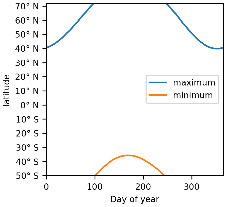
Figure 1Maximum and minimum latitude of TROPOMI nadir pixels according to the SZA cutoff criterion of 65∘ as a function of the day of year for the considered latitude range (50∘ S to 72∘ N).
In v2, viewing zenith angles (VZAs) are restricted additionally to values below 56∘, avoiding less favorable viewing conditions at the swath edges. In addition, this selection limits the maximum pixel width (across track) to 11 km. In contrast to v1, no regional preselection of potentially polluted regions was made in v2. Only high latitudes (north from 72∘ N or south from 50∘ S) are skipped directly.
3.2 Effective plume height
In this study, horizontal transport is described by horizontal wind fields at a fixed “plume height”. This is a simplifying assumption, as the emissions take place at a stack height of about 200 m but are uplifted and vertically mixed within the boundary layer during downwind transport.
For the quantification of point source emissions, the focus of this study is set to the horizontal transport close to the point source, where spatial gradients are largest. As shown in Kuhn et al. (2022), power plant emissions at 200 m stack height quickly rise to about 500 m within the first hundred meters. Brunner et al. (2019) investigated the effective height of CO2 emissions for atmospheric transport simulations. This is closely related to the question of which altitude has to be considered in order to describe horizontal transport of a fresh power plant plume appropriately. For summer around noon, they report mean effective heights of about 450 m (with a long tail towards larger values).
In this study, we assume an effective plume height of 500 m a.g.l. For individual stations and specific meteorological situations, systematic deviations might occur. In order to quantify the impact of this assumption, we thus also performed the analysis for a plume height of 300 m (see Sect. 3.12.3).
ERA5 wind fields are vertically interpolated to the assumed plume height (Sect. 3.5). In addition, the AMF correction is applied consistently for the same height (Sect. 3.3).
3.3 Air mass factor correction
The AMF and the averaging kernel (AK), reflecting the total and height-dependent sensitivity of satellite measurements for atmospheric trace gases, are key concepts for the interpretation and quantification of trace gas column densities (Eskes and Boersma, 2003). The operational NO2 TVCD is based on AMFs calculated for an a priori vertical profiles of NO2 taken from a global chemistry model. With the AK provided in the TROPOMI data, i.e., the ratio of height-dependent (box-)AMF to the total AMF, the AMF can be adjusted to a different a posteriori vertical profile (Eskes and Boersma, 2003).
In polluted regions, vertical profiles of NO2 are generally highly complex, and a local NOx source can typically not be adequately represented by global chemistry models with comparably coarse spatial resolution. In the case of NOx point sources, however, the horizontal gradient in NO2 is basically sensitive to the NO2 excess added by the point source. Any “background” NO2 (which might be considerably polluted in densely populated regions) is intrinsically corrected for by the spatial derivative, i.e., the difference between NO2 levels upwind and downwind of the point source.
Thus, for the quantification of point source emissions, the AMF has to be corrected with respect to the NO2 excess added by the point source. Hence, we apply an AMF scaling factor
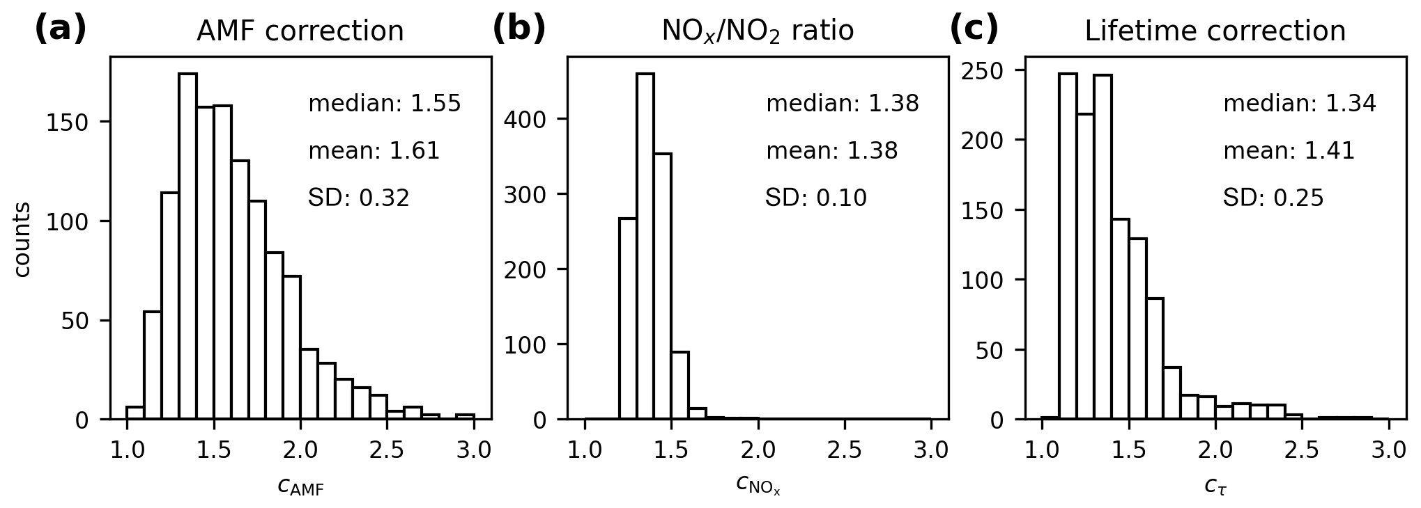
where AMFPAL is the tropospheric AMF applied in the PAL product, and AMFplume is calculated from the AK based on a delta-peak profile at plume height (default 500 m); i.e., cAMF reflects how much higher the plume AMF is compared to the a priori value. For the detected point sources, the AMF correction is about 1.61 ± 0.32. Figure 2a displays the respective frequency distribution for the point sources listed in the v2 catalog.
Note that in v1, no AMF correction was applied, as the AK provided in the TROPOMI data used in v1 was based on a cloud height that was reported to be biased low (Compernolle et al., 2019; van Geffen et al., 2022), as discussed in Beirle et al. (2021), while no reprocessed dataset was available at that time.
3.4 Upscaling NO2 to NOx
As in v1, the TROPOMI NO2 TVCD is upscaled to NOx by the scaling factor , which is calculated based on the photo-stationary state (PSS) according to
where
-
the photolysis frequency of NO2 J is parameterized as s−1, as proposed by Dickerson et al. (1982), with SZA taken from TROPOMI;
-
the rate constant k for the reaction of [NO] with [O3] is parameterized as (in cm3 molec−1 s−1), as recommended by IUPAC (2013), with temperature T (in kelvin) from ERA5; and
-
[O3] is taken from a multi-year climatology modeled by ESCiMo (see Sect. 2.3).
While PSS might not be fulfilled close to a power plant stack, it is a reasonable assumption on the spatial scales of TROPOMI pixel size (of the order of 5 km) and particularly for the 15 km radius considered for emission quantification (see Sect. 5.3.1 for further discussion).
For the detected point sources, the ratio was found to be about 1.38 ± 0.10. Figure 2b displays the respective frequency distribution. Note that these values of the ratio are not representing average values but refer to cloud-free conditions close to local noon with SZA < 65∘. For further discussion on the spatial distribution of the ratio, see Beirle et al. (2021), where also a global map is presented.
Below, we consider TVCDs of NOx (denoted as V) which are derived from the PAL NO2 TVCD multiplied by cAMF and .
3.5 Advection versus divergence
In Beirle et al. (2019, 2021), the divergence of the horizontal flux F=wV, with horizontal wind fields w and TVCD V, was calculated:
According to product rule, this equals
The first term is the scalar product of the (horizontal) wind vector and the spatial gradient of the TVCD; in meteorology, this is denoted as “advection” in the sense of “the rate of change of the value of the advected property” (American Meteorological Society, 2012). Below, we use the term advection in this sense for the quantity A:
The second term of Eq. (4) reflects the divergence of wind fields scaled by the TVCD. However, as we are interested in flux changes caused by local NOx emissions rather than by non-vanishing divergence of the wind fields, we now directly calculate the advection according to Eq. (5), as also proposed recently by Sun (2022). Therefore, in v2, the impact of non-vanishing divergence of the wind field is explicitly skipped. However, the resulting mean maps of A and D are very similar, as the temporal mean divergence of wind fields (at 500 m above ground) is negligibly small. Thus, the switch from “divergence” to “advection” is rather a change in terminology but appropriately describes the retrieval steps that have actually been implemented in the processing of the v2 catalog.
As in v1 of the catalog, only observations with wind speeds above 2 m s−1 are considered in the further processing.
3.6 Derivative on the TROPOMI grid
In Beirle et al. (2019, 2021), spatial derivatives were calculated after gridding the TROPOMI data on a regular latitude–longitude grid. In contrast, de Foy and Schauer (2022) proposed to calculate spatial derivatives directly on the native TROPOMI grid (along-track and across-track).
The main advantage of taking derivatives directly on the TROPOMI grid is the handling of gaps (e.g., due to cloud masking): on the TROPOMI grid, a gap in TVCD just results in a gap in the respective gradient; in contrast, if the derivative is calculated for a temporal mean on a regular latitude–longitude grid, as in v1, gaps on individual days cause steps in the mean distribution, resulting in spikes in the spatial derivatives.
In order to calculate the advection on the TROPOMI grid, the following steps are performed:
-
For each TROPOMI pixel, horizontal wind fields from ERA5 are interpolated linearly to the assumed plume altitude (default: 500 m above ground) and to the observation time and latitude and longitude of the TROPOMI pixel center.
-
The horizontal wind vector is transformed to TROPOMI coordinates by rotation according to the TROPOMI pixel orientation.
-
The gradient of the TVCD on the TROPOMI grid is calculated for each TROPOMI pixel, requiring valid TVCDs for all along-track and across-track neighbor pixels. As the TROPOMI grid becomes skewed towards the swath edges, the respective transformations of the gradient operator for skewed coordinates are applied, resulting in a scaling factor of , with ϕ being the deviation from orthogonality (see https://en.wikipedia.org/wiki/Skew_coordinates, last access: 27 June 2023).
-
The advection is calculated as the scalar product of the wind vector and the gradient of the TVCD, both defined on the TROPOMI grid. The resulting scalar A is independent from the coordinate system.
3.7 Topographic correction
In v1, systematic artifacts of the divergence map were reported over mountains with high tropospheric TVCDs, in particular over parts of China, which hinders the identification and quantification of NOx point sources. These artifacts were explained by inaccurate wind fields over mountains in Beirle et al. (2021). However, a recent study by Sun (2022) shows that these patterns are rather caused by 3D transport effects which have been ignored so far in the simplified 2D divergence approach.
Sun (2022) derives a “topography-wind” term in order to correct for this effect:
with NOx TVCD V (without AMF correction), NOx scale height Hsh, surface wind speed w0, and surface elevation z0.
We include this correction term in order to account for topographic effects: Ctopo is calculated for each TROPOMI pixel based on the surface elevation and surface wind speed (10 m) provided in the PAL NO2 data and assuming an a priori NOx scale height of 1 km.
The topography-corrected advection is then derived as
where the scaling factor f is derived empirically as 1.5 (corresponding to a net NOx scale height of km = 667 m) in order to minimize topography effects, as shown in Appendix A. From now on, we denote the topography-corrected advection as A* in labels and equations but still refer to it as “advection” in the text for the sake of simplicity; i.e., the application of the topographic correction is implied below.
3.8 Gridding and averaging
For each TROPOMI orbit, the NOx advection derived on the TROPOMI grid, as well as all other relevant variables like NOx and AMF scaling factors, wind speed, or topographic correction, is re-gridded on a regular lat–long grid with 0.025∘ resolution, considering latitudes from 50∘ S to 72∘ N. Afterwards, temporal averages are calculated for daily, monthly, and annual periods as well as for the complete time series covered by the PAL NO2 product (May 2018–November 2021).
The temporal mean advection map of A* is the basis for the identification and quantification of NOx point sources. A high-resolution map is provided in the Supplement. Note that regions with less than 10 % temporal coverage have been skipped. This criterion removes regions with poor statistics of the filtered data, caused by frequent cloud cover, snow and ice cover, and/or low wind speeds.
3.9 Point source identification
As in Beirle et al. (2021), point sources are identified in an automated iterative process in which local maxima of the temporal mean (May 2018–November 2021) advection map are successively checked for being point sources. The criteria for classifying potential point source candidates have been extended and modified, as explained in detail below.
In v2, a default radius 15 km is considered for the quantification of NOx emissions, in contrast to 22 km in v1. This reduces the skipping of point sources due to interfering sources nearby. A new quantity used during the categorization procedure is the “peak area fraction” which is just defined as the percentage of grid pixels (on 0.025∘ grid) within a given radius around the candidate that have advection values above a threshold (here: 30 % of the local maximum). This quantity helps to identify single spikes (with very low peak area fraction) as artifacts, as well as area sources (with large peak area fraction).
Point sources are identified by a fully automated iterative procedure, in which a “candidate” is identified and classified in each iteration step:
-
The candidate location is defined by the absolute maximum of the advection map. Figure 3a displays the maximum advection value as a function of the iteration step.
-
The following criteria are checked successively for the candidate until a classification is made:
-
If the distance between candidate and the edge of the advection map is less than 30 km, the candidate is categorized as “edge”.
-
If more than 25 % of the grid pixels within 15 km around the candidate are missing, it is categorized as “gap”.
-
Systematic biases in, e.g., the assumed plume height, ERA5 wind direction, or non-steady-state effects can cause dipole-like patterns of enhanced positive and negative advection. In order to avoid such artifacts to be interpreted as point sources, candidates with large negative advection values nearby are skipped. As these effects can affect larger areas, the search for negative values is extended over a larger distance: if negative values are found within 30 km around the candidate with an absolute value larger than 50 % of the candidates maximum, it is categorized as “negative”. In addition to identifying dipole patterns, this criterion also adapts to the local noise level in the advection map and prevents the interpretation of a local maximum just caused by noise as a point source.
-
If the peak area fraction within 5 km is lower than 80 %, the candidate is classified as “none”. This reflects spikes that do not correspond to the expected extent of the peak in advection map according to TROPOMI spatial resolution of the order of 5 km. Note that this category is very rare: only 191 out of 50 000 candidates fall into this category (Fig. 4b).
-
If the peak area fraction within 15 km is above 45 %, indicating a spatially extended advection peak, the candidate is categorized as “area source”. Such broad peaks in the advection map might be caused by cities (vehicle emissions) as well as extended industrialized areas or multiple interfering point sources within about 10–20 km distance.
-
Otherwise, the candidate is classified as a point source (“ps”).
-
-
Before the next iteration step, the candidate is removed from the advection map by setting all positive values within 15 km (30 km in the case of the “negative” category) to not a number (NaN). Negative values are kept in the advection map such that they can still trigger the “negative” category for following candidates in the vicinity.
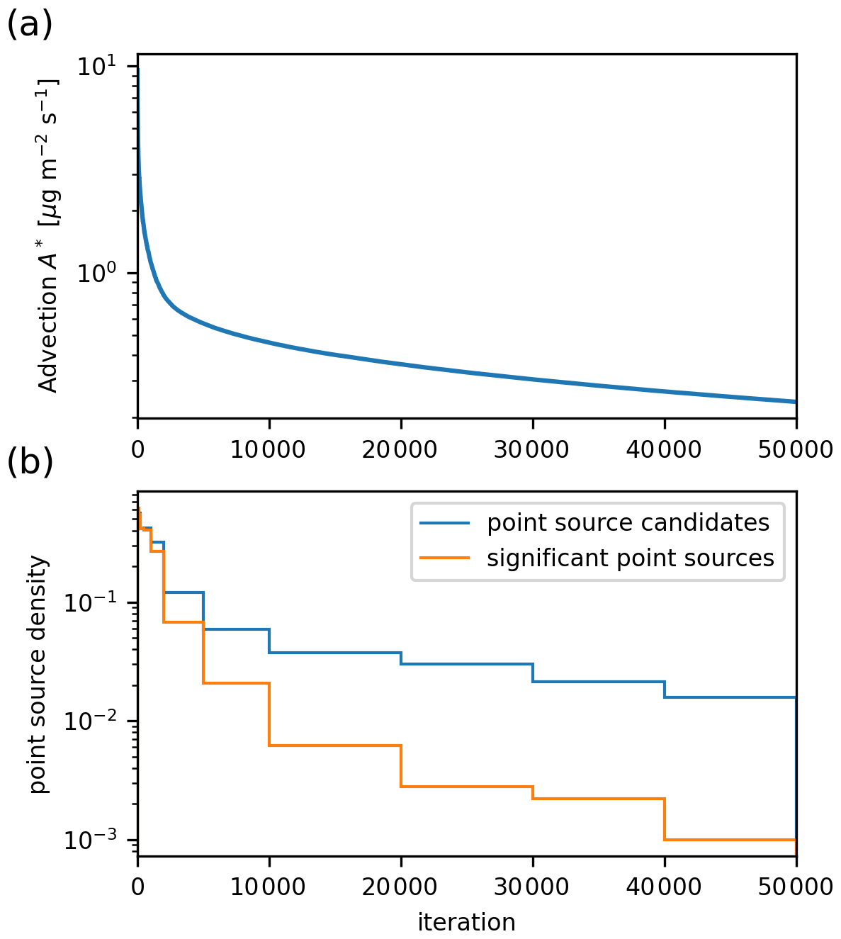
Figure 3Iterative candidate classification. (a) Local maximum advection as a function of the iteration step. (b) Density of point source candidates (blue) and significant point sources (orange; see Sect. 3.11) per iteration as a function of the iteration step.
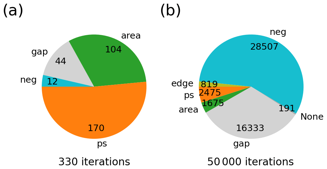
Figure 4Frequency distribution of the different categories for (a) the first 330 iterations, where maximum advection is > 2 µg m−2 s−1, and (b) for all 50 000 iterations.
For the v2 catalog, 50 000 candidates have been processed. In the beginning, a high fraction of candidates is classified as a point source (Figs. 3b and 4a). For the first 330 iterations, where maximum advection is >2 µg m−2 s−1, 52 % of all candidates are found to be point sources and another 32 % as area sources. In later iteration steps, while maximum advection decreases by almost 2 orders of magnitude, the majority of candidates is classified as gap (initially due to actual gaps in the input data, later due to the removal of prior candidates nearby) or negative (due to artificial dipolar patterns and due to maxima close to the local advection noise level). Within iterations 40 000–50 000, only 10 significant point sources have been found, and further iterations are not meaningful.
3.10 Point source quantification
For the candidates identified as point source, the respective NOx emissions are quantified by spatial integration of the advection map (Sect. 3.10.1), corrected for NOx lifetime (Sect. 3.10.2).
3.10.1 Spatial integration
In v1, a 2D Gaussian was fitted to the mean divergence map for the quantification of point source emissions. However, this procedure requires good statistics (i.e., long-term means) and a sufficiently large spatial range (22 km radius in Beirle et al., 2021) in order to perform stable fits. Moreover, an additive background was included as a fit parameter in the model function. This counteracts the paradigm of the advection (or divergence) method being sensitive to local emissions (excess NOx) and that the background is already corrected for by the spatial derivative.
Thus, we have simplified the calculation of emissions by just integrating the advection map spatially 15 km around the point source location. This radius has been found to be a good compromise as it is large enough to cover the observed point source peaks in the advection map, as illustrated exemplarily for some selected point sources in Fig. 5. On the other hand, neighboring sources can still be discriminated. For instance, the Weisweiler power plant southwest of Niederaußem and Neurath (Fig. 5b) is automatically detected as separate point source which was not the case in v1 of the catalog that was based on the Gaussian fit within 22 km radius. In addition, this simple and robust procedure does not rely on fit convergence and thus also works for higher spatial noise levels, i.e., for shorter temporal averages like monthly means.
We checked the impact of the simplified emission estimate procedure by applying it also to v1 of the catalog. Resulting emissions from Gaussian fit vs. spatial integration agree well with a correlation coefficient of r = 0.96, whereby emissions from spatial integration are higher by 12 % on average.
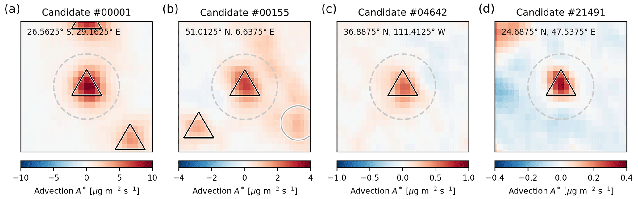
Figure 5Sample maps of the temporal mean advection, corrected for topography, for (a) the first candidate classified as point source, i.e., the Secunda coal liquefier (South Africa), (b) Niederaußem and Neurath power plants (Germany; see also Sect. 4.2.1), (c) the Navajo power plant (USA; see also Sect. 4.2.2), and (d) the candidate with the lowest derived emissions, i.e., the Al Yamama cement factory (Saudi Arabia). Results of the candidate classification are indicated by triangles for point sources and circles for area sources. The large dashed circle reflects the 15 km radius used for the candidate classification procedure as well as for spatial integration. Note the different color scales.
3.10.2 Lifetime correction
Tropospheric NOx has a rather short lifetime of the order of some hours. Thus, the positive advection caused by a point source is opposed by the chemical loss of NOx within the downwind plume.
In Beirle et al. (2019), it was proposed to correct for the NOx loss by adding a sink term to D by assuming a first-order lifetime τ. However, this approach had the disadvantage that the high-contrast maps of D (or A) were overlaid by the spatial distribution of the mean VCD V which is smeared out spatially. Consequently, the sharp contrast of D (or A) was lost, and for integrated emissions, larger scales than a 15 km radius had to be considered. Thus, in Beirle et al. (2021), no lifetime correction was applied, as the correction was assumed to be small for strong point sources, based on a constant lifetime of 4 h. However, there are indications that the lifetime of tropospheric NOx can be significantly shorter than that. For instance, Goldberg et al. (2019) report a lifetime of only 1.5 h for the Colstrip power plant. Recently, Lange et al. (2022) systematically investigated NOx lifetimes worldwide and found typical values of about 2 h for low latitudes up to about 4–6 h at higher latitudes.
In v2 of the catalog, we apply an alternative approach for correcting for the chemical loss of NOx, which is based on the residence time tr of the emitted NOx within the 15 km radius:
with the mean wind speed w.
The lifetime correction has to compensate for the integrated loss within the residence time, which results in a scaling factor
as explained in more detail in Appendix B. A scaling factor of, e.g., cτ = 1.25, thus compensates for a reduction to 80 % of the emitted NOx due to the chemical loss within the residence time.
For the calculation of cτ, we use the dependency of τ on latitude as derived by Lange et al. (2022):
with τ in hours and latitude in units of degree. Note that the seasonal dependency of the NOx lifetime has been found to be rather weak (probably due to the focus on cloud-free conditions around noon), while seasonal estimates have larger uncertainties due to reduced statistics (Lange et al., 2022). Thus, we do not consider a possible seasonal dependency of the NOx lifetime explicitly. In addition, high variability of lifetimes at different locations of similar latitude has been reported, e.g., in Laughner and Cohen (2019). Thus we assume a rather large uncertainty of 50 % for τ (see Sect. 3.12.1).
For the detected point sources, the resulting lifetime correction factor is about 1.40 ± 0.24. Figure 2c displays the respective frequency distribution.
3.10.3 Final emission estimate
Total emissions of a given point source are derived from spatial integration of A* around r= 15 km, scaled by the lifetime correction factor:
with ∘ denoting the spatial integration over a circle with 15 km radius. Note that the spatial integration of the gridded advection map is realized by summing up the advection values multiplied by the pixel area for all grid pixels within the 15 km radius.
3.11 Selection of significant point sources
The iterative classification algorithm yields 2475 point source candidates. For v2 of the catalog, we select significant and reliable point sources by different criteria, i.e., the detection limit, the integration error, the contribution from topographic correction, and the temporal persistence of the derived emissions.
3.11.1 Detection limit
In Beirle et al. (2019), the detection limit (DL) for NOx point sources was estimated to be “0.11 kg s−1 down to 0.03 kg s−1 for ideal conditions.” From exemplary visible inspection, we found that these thresholds are meaningful for the updated results as well and apply them in order to consider a point source as significant for v2 of the catalog.
“Ideal conditions” are found for cloud-free scenes with high surface reflectivity, like for the Saudi Arabian capital Riyadh (Beirle et al., 2019). We thus apply a simple albedo mask in order to decide whether a candidate faces desert-like conditions or not: for all candidates with a minimum LER above 8 %, a DL of 0.03 kg s−1 is set, whereas for all other sites, DL is taken as 0.11 kg s−1. In Fig. 8, the regions with DL of 0.03 kg s−1 are marked.
3.11.2 Integration error
For each grid pixel, the temporal mean and standard deviation of all gridded quantities are calculated. This allows the standard mean error of the mean advection for each grid pixel to be calculated and thus also the statistical error of the spatial integration. Point sources are only considered to be significant if the relative error of spatial integration is below 30 %.
3.11.3 Topographic correction
The topographic correction has been found to improve the mean advection map and thus the point source emission estimate. However, the empirically derived scaling factor (Appendix A) has been selected as a compromise and does not work perfectly everywhere; on the contrary, some new artifacts are introduced in the advection map over mountains downwind of strong sources. In order to avoid the misinterpretation of such topographic effects as point sources, we consider point sources to be significant only if the topographic correction contributes less than 50 % to the integrated emissions.
3.11.4 Temporal persistence
For each detected point source, a time series of monthly emissions is calculated according to Eq. (11). Note that the monthly mean advection is usually too noisy in order to perform the automated point source detection; for the known point source locations derived for the full-time advection mean, however, the emissions can still be calculated on a monthly basis for most cases (with higher uncertainties).
The monthly mean emissions are then checked for significance, i.e., emission values above the detection limit with relative integration errors below 30 %. In the final catalog, information on the number of months with significant emissions is provided. We consider this quantity as a measure for temporal persistence, i.e., how persistent the point source is over time. Generally, the number of months with significant detection is the lower the weaker a point source is, as noise becomes more important. But low persistence might also indicate that a power plant was switched off during the considered period, like the Navajo power plant in the USA, as shown in Sect. 4.2.2.
Very low persistence of values down to 1, however, can also be related to exceptional events like strong biomass burning, e.g., in South America or Australia. For v2 of the catalog, we only consider point sources that show significant emissions for at least 6 months.
From the 2475 point source candidates, 1139 significant point sources remain after applying these criteria. For the catalog of NOx point sources, the remaining candidates (which are sorted by maximum advection) are re-sorted by the determined emissions (spatially integrated and lifetime-corrected) and are assigned by a “rank” starting at 1.
3.12 Errors
The v2 catalog provides an error estimate for each derived emission. This error is calculated from the estimated uncertainties of the involved retrieval steps, as detailed below.
Note that there are further uncertainties that may cause a systematic bias of the derived emissions but cannot be easily quantified and are thus not included in the quantitative error estimate of the catalog. A discussion of these errors is provided in Sect. 5.3.
3.12.1 Scaling factors
For the scaling factors for the ratio and the AMF correction, the uncertainty is estimated from the standard error of the temporal mean, i.e., the standard deviation divided by the square root of the sample size, separately for each point source. The uncertainty of the lifetime correction is calculated by error propagation applied to Eqs. (8) and (9), with the statistical error of the temporal mean of w and assuming a relative uncertainty of 50 % for the lifetime parameterization with latitude.
3.12.2 Spatial integration
The error of spatial integration is determined via the statistical error of the temporal mean for each grid pixel (see Sect. 3.11.2).
3.12.3 Plume height
For the plume height, an a priori value has to be assumed. The v2 catalog is based on a plume height of 500 m above ground. This height is used for two different retrieval steps:
-
the application of the AMF correction and
-
the interpolation of wind fields.
In order to estimate the impact of the a priori assumption, we also performed the analysis for a plume height of 300 m and consider the difference as the uncertainty proxy. Note that in Beirle et al. (2019), similar case studies were used in order to estimate the impact of height used for wind interpolation, whereby the simultaneous impact on the AMF was ignored therein. However, explicit comparison of the AMF correction factors for plume heights of 300 and 500 m reveals that the effect on AMF is very small (about 1 %). Thus, the main impact of assumed plume height is indeed that on wind fields.
3.12.4 Topographic correction
We apply the topographic correction with a scaling factor f of 1.5 and a relative uncertainty of 33 % (see Appendix A). This uncertainty is propagated to the corrected advection map according to Eq. (7).
3.12.5 Total error
Following the propagation of errors, the total error is determined from the individual contributions listed above.
Figure 6 displays histograms of the different error components and the total error. Uncertainties of scaling factors for NOx and AMF as well as spatial integration error are small (<10 %). The lifetime correction has an uncertainty of about 10 %–20 % but can also be considerably larger for some point sources. The impact of the a priori height used for the interpolation of wind fields is about 10 %, similar to that reported in Beirle et al. (2019). The topographic correction is below 2.5 % for most point sources but can become significant for point sources in mountain areas. Total uncertainties are typically 20 %–40 %.
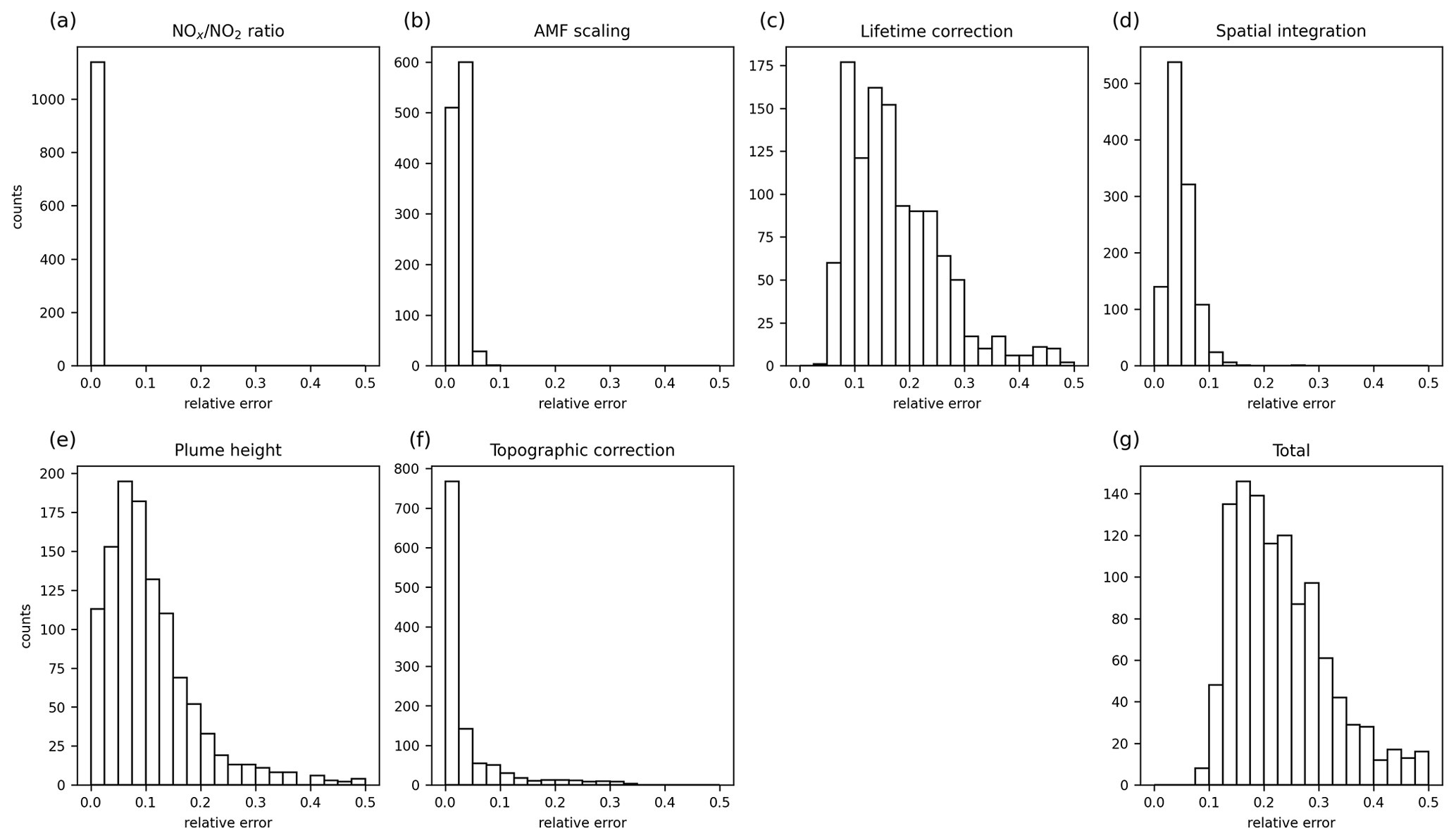
Figure 6Histograms of relative errors for (a) the NOx scaling factor, (b) the AMF scaling factor, (c) the lifetime scaling factor, (d) the spatial integration, (e) the impact of a priori plume height, (f) the topographic correction, and (g) the total error for the detected point sources.
3.13 External information
In order to provide information about the potential origin of the detected emissions, we add spatial matches within 15 km distance of
-
combustion power plants, as listed in the GPPD, with a capacity above 100 MW, and
-
cities, as listed in WCD, with more than 100 000 inhabitants.
Figure 7 displays the number of point sources with a match in GPPD, WCD, or both. For the top 100 point sources, a matching power plant is found in 89 cases (in 36 cases accompanied by a city). For the complete catalog, there is a power plant nearby still for more than half of the detected point sources, while 194 further point sources can be explained by city emissions like traffic and/or industrial facilities. The remaining 302 point sources without a match in GPPD or WCD can correspond to cement plants, metal smelters, or other industrial facilities outside from cities.
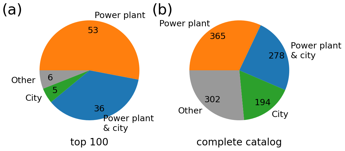
Figure 7Statistic of matching power plants and cities for (a) the top 100 NOx point sources and (b) the full catalog.
3.14 Changes of v2 with respect to Beirle et al. (2021)
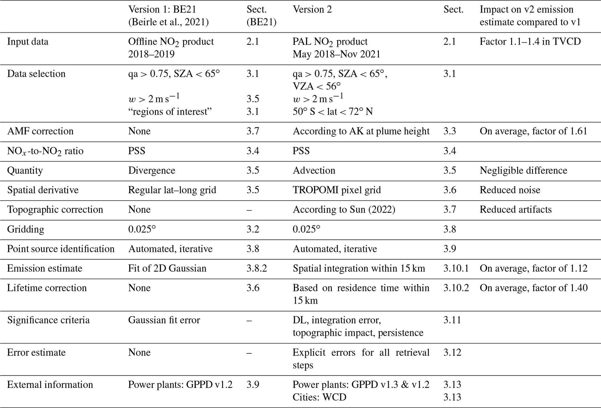
Table 1 provides a comparison of the different steps for v1 and v2 of the catalog, including references to the sections where further details are provided for v1 (Beirle et al., 2021) and v2 (this paper).
The main differences, affecting the updated catalog and in particular the reported NOx emissions, are
-
the usage of the consistently reprocessed TROPOMI NO2 PAL product, with higher NO2 TVCDs;
-
the application of an AMF correction;
-
the calculation of the spatial derivative on the TROPOMI pixel grid, reducing noise levels of the advection map drastically, in particular for regions with regular cloud cover;
-
the correction of topographic effects, which are considerable over mountains for high “background” pollution, like in parts of China or South Korea;
-
the simplification of the quantification of point source emissions by spatial integration, also allowing for estimates based on monthly means;
-
the application of an explicit correction of the NOx loss within 15 km around the point source;
-
the calculation of errors for each point source.
The spatial derivative on the TROPOMI grid and the application of the topographic correction result in improved advection maps with lower noise and fewer artifacts, allowing for the automated detection of far more point sources (1139 compared to 451 in v1). The higher TVCDs (factor of 1.1–1.4) and the application of corrections for AMF and lifetime (factors of about 1.6 and 1.4, respectively) result in higher NOx emission estimates by a factor of about 3, resolving the low bias that has been found for the emissions reported in v1 (Beirle et al., 2021).
(Beirle et al., 2021)Sun (2022)Table 1Overview of algorithm steps of v2 of the catalog in comparison to v1.
4.1 NOx point source catalog v2
Version 2 of the point source catalog can be found on https://doi.org/10.26050/WDCC/No_xPointEmissionsV2 (Beirle et al., 2023). In addition, it is provided in the Supplement. The catalog provides latitude, longitude, NOx emissions, and uncertainties for the detected point sources. In addition, power plants from GPPD and cities from WCD are added. Also, the number of significant months is provided. Besides the basic catalog for the full period covered by the PAL NO2 product, annual means for each year 2018–2021 are also provided.
The catalog comprises 1139 point sources worldwide. Figure 8 displays an overview of the spatial distribution of detected point sources, where power plant and city matches are color-coded. In the Supplement, regional maps of the detected point sources are provided with the corrected advection map as a background image.
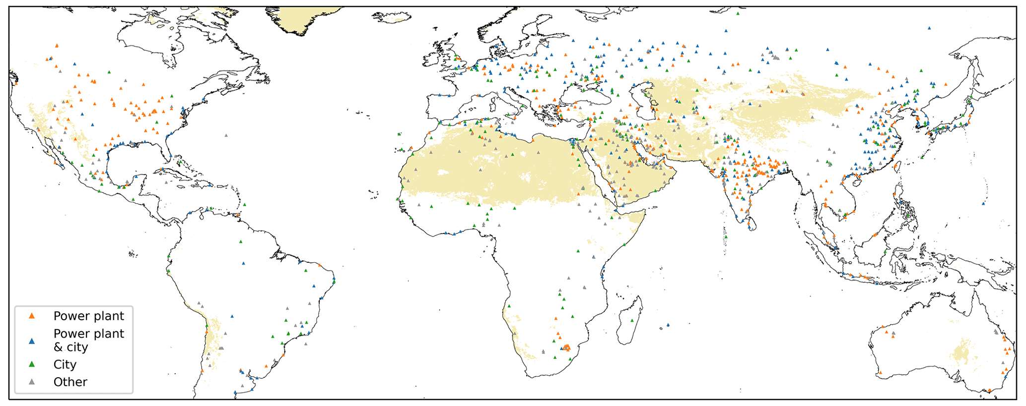
Figure 8Location of point sources listed in v2 of the catalog. Matches in GPPD and/or WCD are indicated by colors as in Fig. 7. The background map highlights regions with high LER, where a detection limit of 0.03 kg s−1 is assumed.
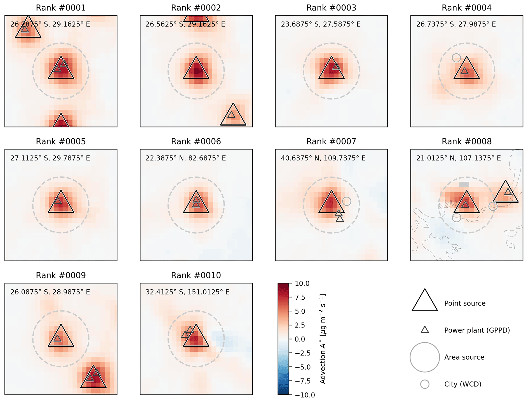
Figure 9Maps of A* for the top 10 NOx point sources listed in the catalog (see Table 2). Markers indicate the location of point sources (triangles) and also candidates that have been discarded as area sources (circles; only for advection above 0.5 µg m−2 s−1). The large dashed circle reflects the 15 km radius used for candidate classification and spatial integration. Small triangles and circles show GPPD power plants and WCD cities, respectively.
Table 2 shows an extract of the v2 catalog. It includes the top 10 emitters worldwide as well as every 100th point source exemplarily. Figures 9 and 10 show the corresponding maps of the corrected advection. Additional tables for regional top 10 emitters are provided in the Supplement for various regions.
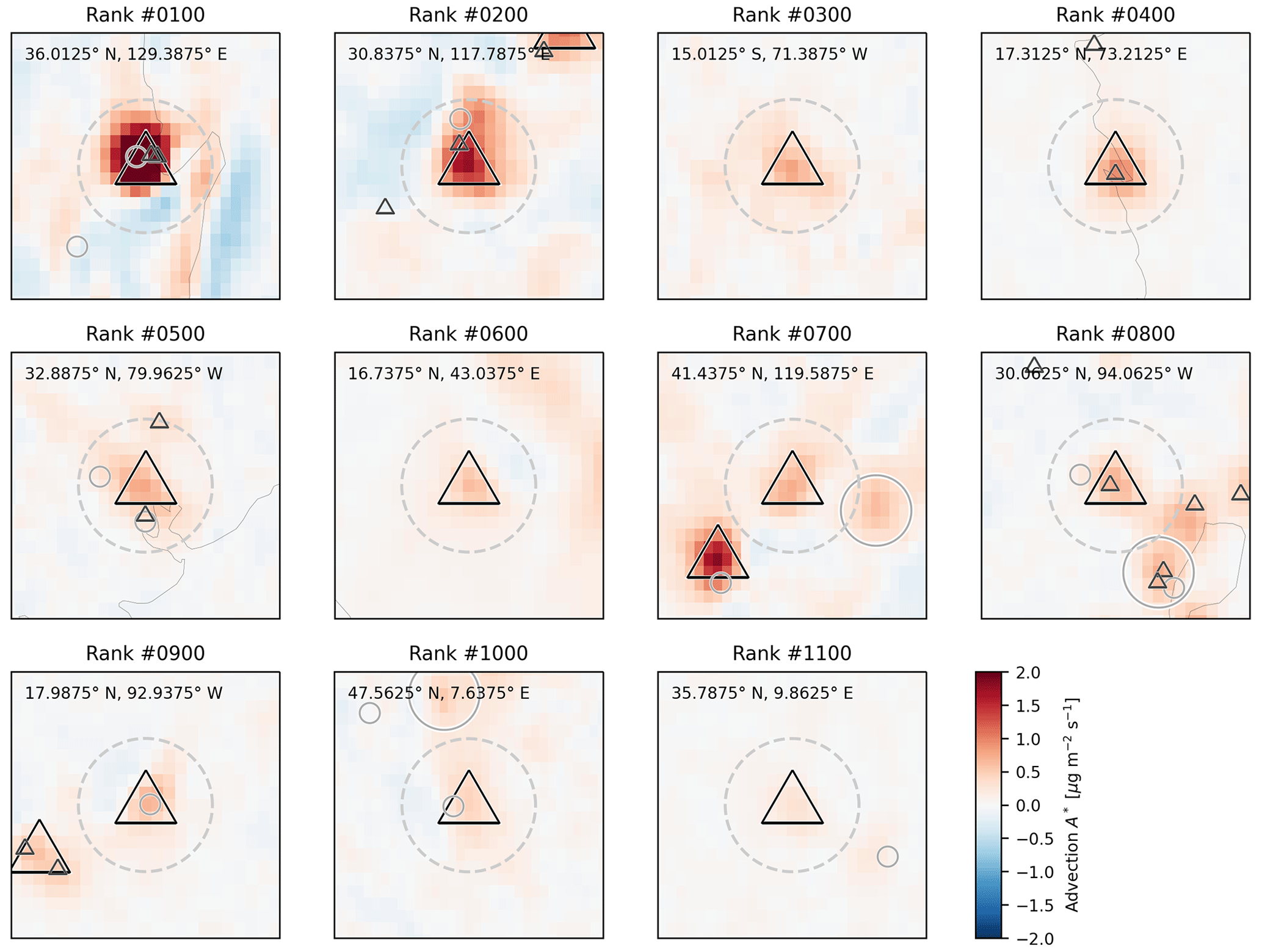
Table 2Extract of the v2 catalog, including rank, latitude, longitude, NOx emissions, and error as well as matching power plants and cities.
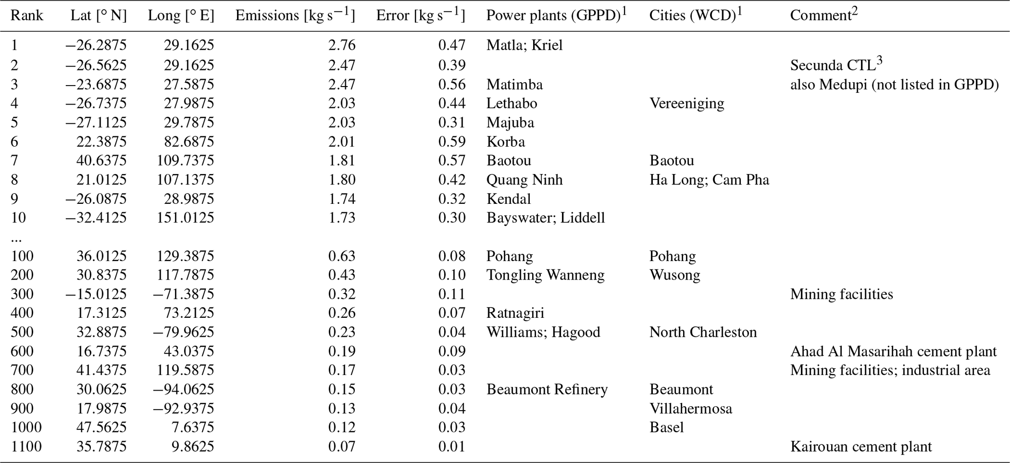
1 Shortened for clarity. 2 Not part of v2 catalog. 3 https://en.wikipedia.org/wiki/Secunda_CTL (last access: 27 June 2023).
As in v1, the global top 5 emitters are all located in South Africa, and all top 10 emitters are related to the combustion of coal. While the overall ranking is similar as in v1, the derived emissions are considerably higher in v2 by a factor of about 3–4 due to the applied corrections and the new emission quantification method.
For five of the point sources listed in Table 2, no match was found in GPPD nor WCD. We checked these point sources manually and added information about the likely NOx source, which were found to be related to coal liquefaction, cement plants, mining activity, and/or industrial areas.
4.2 Validation
We validate the derived NOx emissions by comparison to regional emission datasets: the PRTR for Germany (Sect. 4.2.1) and the eGRID emissions for US power plants (Sect. 4.2.2).
4.2.1 Germany
We compare the NOx emissions of the v2 catalog to PRTR emissions reported by UBA for Germany. Each point source over Germany is merged with all PRTR emissions within 15 km. Table 3 lists an extract of the catalog for Germany, extended with the respective PRTR matches. For all point sources over Germany listed in the v2 catalog, matches with GPPD as well as PRTR sources were found.
Table 3Catalog v2 extract for point sources detected in Germany. In addition, matches with PRTR sources are added for comparison.
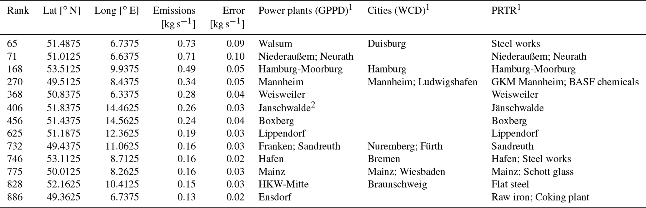
1 Shortened for clarity. 2 Misspelled in GPPD; should be “Jänschwalde”.
As PRTR emissions are reported on annual basis (available for 2018–2020), we compare the annual catalog emissions to the integrated PRTR emissions within 15 km for the respective year. In Fig. 11, the catalog emissions are compared to matching PRTR emissions. A Pearson correlation coefficient of 0.81 was found between annual emissions from v2 catalog and PRTR. The ratio of mean catalog to mean PRTR emissions over all point sources and years was found to be 1.14.
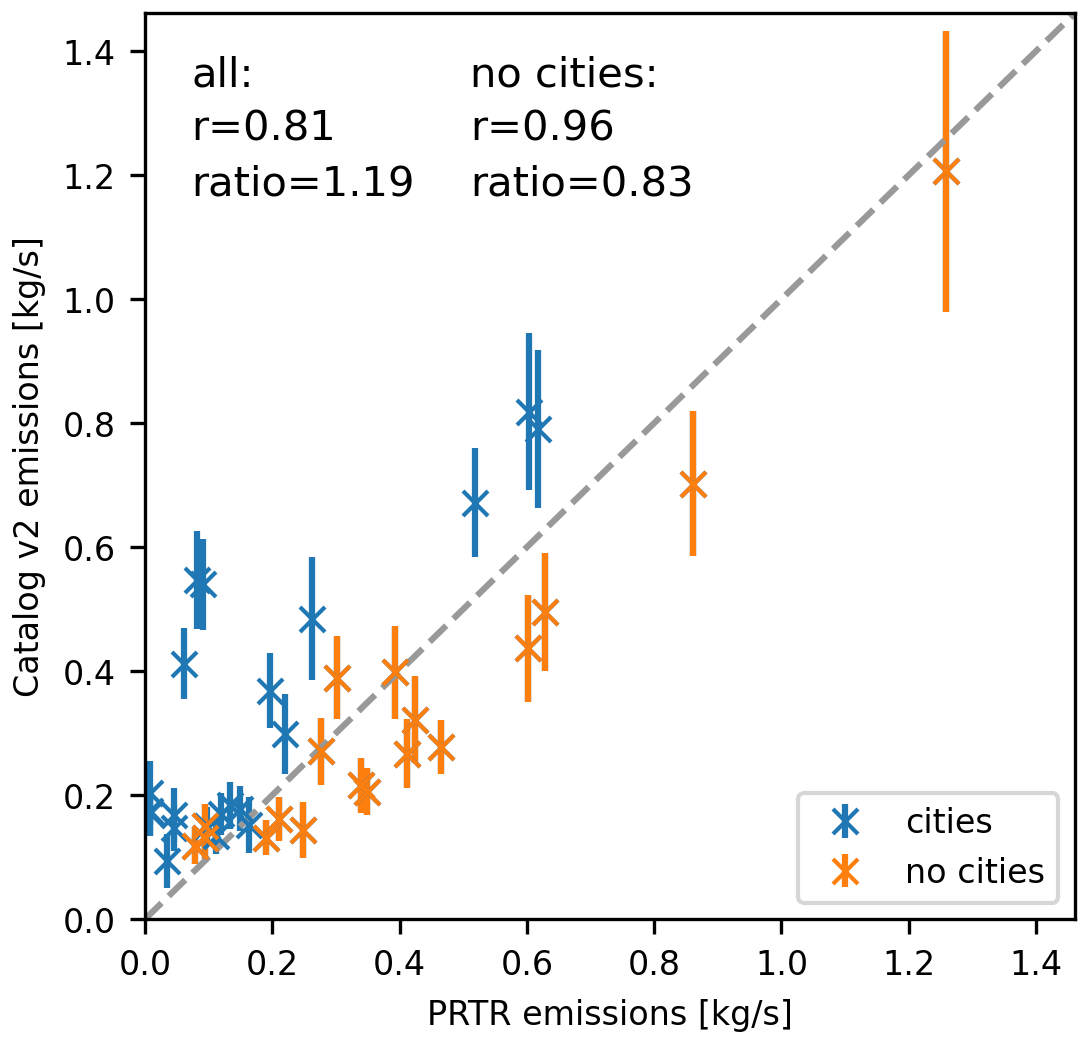
Figure 11Comparison of annual mean NOx emissions from v2 catalog (y axis) to emissions reported in PRTR, added up within 15 km radius (x axis), for Germany. Error bars reflect the errors given in the v2 catalog. Correlation coefficients r and the ratio of mean emissions (v2 versus PRTR) are provided in the figure based on all found point sources as well as for the subset excluding point sources near cities. Note that for each considered point source there are up to three data points displayed, representing annual means for 2018, 2019, and 2020, respectively.
For several point sources, however, interference with other emissions (in particular from traffic) has to be expected due to nearby cities, causing a high bias of the catalog emissions. Thus, we also only performed a comparison for point sources without large cities nearby. This selection of six point sources (mostly lignite power plants) increases the correlation to 0.96, while the ratio of emissions decreases to 0.83; i.e., catalog emissions are on average 17 % lower than those reported in PRTR.
The highest annual mean emissions of 1.2 kg s−1 were found for the lignite power plants Niederaußem and Neurath, catalog rank 71, in the year 2018. In 2019 and 2020, these emissions decreased to 0.7 and 0.5 kg s−1, respectively, in the catalog. This decrease is also reflected in the annual maps of A* (Fig. 12). A similar reduction is reported in PRTR as well.
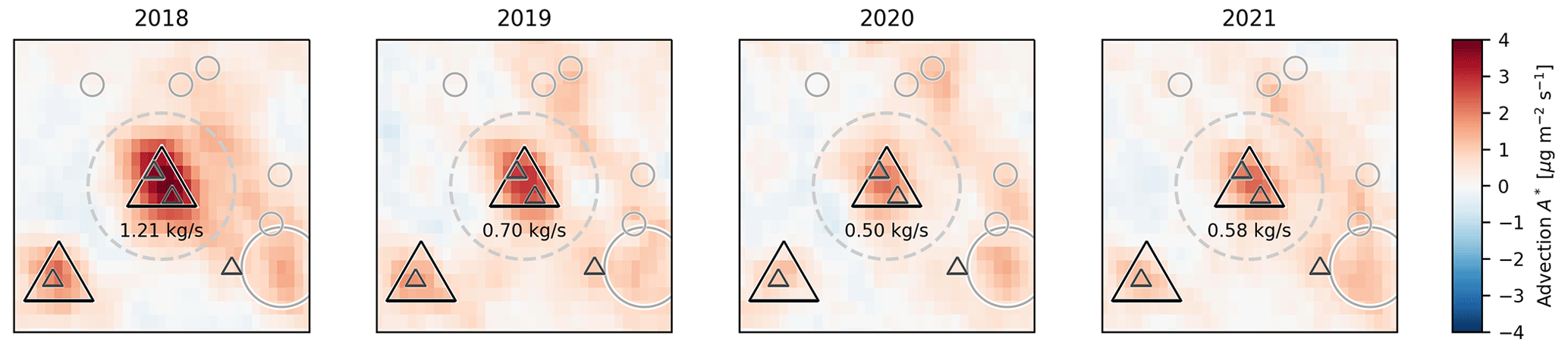
Note that there is one additional point source listed in PRTR with an emission larger than the assumed detection limit of 0.11 kg s−1 which is not included in the v2 catalog, i.e., the lignite power plant “Schwarze Pumpe” (51.536∘ N, 14.354∘ E). The location of Schwarze Pumpe was indeed detected as a point source candidate but was classified as “gap” due to its vicinity to the “Boxberg” power plant at 18 km distance.
4.2.2 USA
The eGRID dataset lists NOx emissions related to power generation but does not cover other NOx sources from cement plants or metal, chemical, and mineral industries. Thus, it has to be expected that the catalog emissions are higher than those reported by EPA whenever significant emissions from cities or industrial activities other than power generation occur within 15 km.
For a meaningful comparison between the v2 catalog and eGRID, we thus focus on
-
point sources that do not coincide with a large city and
-
eGRID emissions above 0.11 kg s−1.
This selection keeps 41 point sources. Figure 13 displays the corresponding comparison of annual NOx emissions between eGRID and the v2 catalog, resulting in a correlation coefficient of 0.64 and a ratio of mean emissions of 0.78.
In some cases, catalog emissions are larger than those reported by eGRID, probably due to interfering emissions from sources other than power plants. In a few cases, the catalog emissions are considerably lower than eGRID.
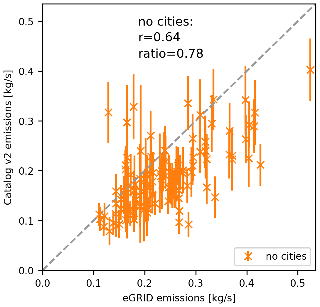
Figure 13Comparison of annual mean NOx emissions from the v2 catalog (y axis) to emissions reported in eGRID, added up within 15 km radius (x axis), for the USA. Point sources close to cities are skipped, as well as eGRID values below 0.11 kg s−1. Error bars reflect the errors given in v2. Correlation coefficients r and the ratio of mean emissions (v2 versus eGRID) are displayed in the figure. Note that for each considered point source there are up to three data points displayed, representing annual means for 2018, 2019, and 2020, respectively.
The Navajo power plant was one of the top NOx emitters in 2019 in the USA but is only listed at rank no. 890 in the v2 catalog. This is due to the shutdown of the Navajo power plant at the end of 2019, which also leads to Navajo being skipped from GPPD v1.3. This shutdown is well reflected in the annual emissions in v2 of the catalog (Fig. 14).
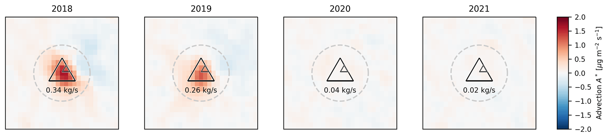
Figure 14Maps of A* for catalog rank no. 890 (36.8875∘ N, 111.4125∘ W), corresponding to the Navajo coal power plant. The shutdown at the end of 2019 results in emissions close to zero in 2020 and 2021. Markers as in Fig. 9.
In eGRID, there are 38 further power plants listed with emissions above 0.11 kg s−1 that are not listed in the catalog. A total of 36 of these power plants were identified as candidates during the iterative point source detection algorithm. In 26 cases, the candidates were indeed identified as point sources, which however were not found to be significant by the strict criteria defined in Sect. 3.11 and are thus not listed in the catalog. The remaining candidates were classified as area, gap, or negative.
5.1 Catalog v2
The updated NOx catalog involves several improvements compared to v1. The calculation of the derivative on the TROPOMI pixel grid avoids spikes and reduces the noise of temporal mean maps, in particular for regions that are regularly affected by clouds. The explicit correction of topography reduces systematic artifacts over mountains. These improvements lead to a higher-quality map of the corrected advection which enables the automated detection of far more point sources (1139) than for v1 (451).
Due to the reprocessed TROPOMI NO2 data, the applied corrections for AMF and lifetime, and the new quantification scheme of point source NOx emissions, the listed emissions are now far more realistic and agree reasonably well with reported bottom-up emissions from governmental inventories.
Thus, the v2 catalog actually provides valuable information worldwide, concerning not only the existence and location of NOx point sources but also the respective NOx emissions. This is of particular relevance for countries where accurate emission data for point sources are not available.
5.2 Missing point sources
The v2 catalog cannot be expected to provide a complete list of NOx point sources worldwide for various reasons.
5.2.1 Data gaps
Point sources could be missing in the catalog if they are not covered by the mean advection map A*. Gaps in A* can be caused by the various selection criteria in particular for SZA, qa value (including a cloud filter), and wind speed and the skipping of grid pixels with less than 10 % temporal coverage in the temporal mean. Note that for calculating the advection for a given pixel on the TROPOMI grid, TVCDs must be valid for all along-track and across-track neighbor pixels.
Consequently, regions with frequent cloud cover or snow and ice are missing in the temporal mean advection map, as can be seen in the regional maps of A* provided in the Supplement. In addition, there are some gaps at desert coastlines, for instance along the Persian Gulf. This is caused by the coarse resolution of the surface albedo map used for the FRESCO cloud product. This issue is expected to improve by the recent update of the processor version v2.4 of the TROPOMI NO2 processor, as the new TROPOMI DLER product with 0.125∘ resolution is used consistently for the cloud (FRESCO) and NO2 retrievals, which will improve the identification of clouded pixels over scenes with strong changes of surface albedo, in particular sand–water transitions.
5.2.2 Spatial interference
Due to the integration within 15 km, point sources close to each other cannot be separated and are likely to be interpreted as one single point source, as for instance the German lignite power plants Niederaußem and Neurath with a distance of 9 km.
For point sources within about 20 km distance from other strong point sources or large cities, spatial interference might cause candidates to be classified as gap or be merged with the city emissions, respectively. For instance, around Riyadh (compare Fig. 3 in Beirle et al., 2019), the automated algorithm successfully detects the power plants PP9 and PP10, both about 25 km afar from the city center, whereas PP7 and PP8 (<20 km distance to city center) are identified as candidates but classified as area sources due to the interference with Riyadh city emissions.
5.2.3 Insignificant point sources
The catalog combines the identification of point sources within a fully automated algorithm with the quantification of the respective NOx emissions. In order to avoid false detection caused by artifacts or noise, stringent criteria are applied in order to identify significant point sources. For the USA, for instance, 26 of the point sources listed in eGRID with emissions above 0.11 kg s−1 were correctly identified as point source candidates but discarded as insignificant and are thus not included in the v2 catalog.
The quantification of NOx emissions by spatial integration of the corrected advection map could be applied to these locations or any other known point source, as well. However, for large parts of the world, such reliable a priori knowledge about the location of point sources is not available. Thus, the v2 catalog focuses on point sources that could be identified from the mean advection map without additional a priori knowledge.
5.3 Systematic errors
The v2 catalog provides error estimates for each point source based on the estimated uncertainties for each retrieval step. In addition, there are potential systematic errors.
5.3.1 Photostationary state
The scaling of NO2 observations to NOx is based on the PSS assumption. This is typically not fulfilled directly at a strong point source due to the added emissions which take place largely in form of NO. These NO emissions are converted to NO2 during plume travel and will thus be detected by the spatial gradient not at but downwind from the source, which would cause a smearing out of the peak in the advection map. Note, however, that the width of the advection plume of about 5 km (Beirle et al., 2021) is of the order of the TROPOMI pixel size, and we do not observe a significant downwind shift in the advection (or divergence) signal.
Nevertheless, we cannot rule out that PSS is not always reached completely within 15 km. Janssen et al. (1988) parameterized the deviation from PSS as a function of downwind distance based on actual aircraft measurements of power plant plumes. The deviations from PSS at 15 km distance have been found to be about 2 % for summer (based on α = 0.25 km−1; see Table 4 in Janssen et al., 1988) up to 24 % in spring and autumn for low background ozone concentrations (based on α = 0.1 km−1; see Table 3 in Janssen et al., 1988), which would cause a corresponding low bias in the estimated emissions.
Increasing the considered radius to, e.g., 20 km would reduce the possible bias of the emission estimate due to non-PSS. On the other hand, this would have other negative impacts:
-
Some of the detected point sources could not be separated any more.
-
The interference with other sources around the point source would increase.
-
The uncertainty of the lifetime correction, which is based on the residence time derived from the wind speed at the point source, would increase.
Thus, we stick to the choice of the 15 km radius in this study.
Additional systematic errors might be introduced by the parameterization of J as a function of the SZA, which so far ignores the impact of the surface albedo, causing a low bias of the [] ratio over deserts of about 5 %. This parameterization might be improved in future studies.
5.3.2 Uncertainties of wind fields
As discussed in Beirle et al. (2019), an error (random as well as systematic) of the assumed wind direction causes a systematic underestimation of the determined flux, as only the wind component parallel to the actual wind direction matters. In Beirle et al. (2019), this effect was estimated to be about 3 % for the city of Riyadh. Larger biases have to be expected over regions with low wind speeds (with higher uncertainties of wind direction) and over mountains (where modeled wind fields are generally more uncertain and the spatial resolution of the meteorological model might not be sufficient).
5.3.3 Mountains
In addition to higher uncertainties in wind fields, 3D effects of transport also come into play as soon as the terrain has spatial gradients. Sun (2022) proposed an explicit correction term for this effect. in which the surface concentration of NOx is estimated as the ratio of the tropospheric column and an a priori NOx scale height. Here, we apply the correction term (Eq. 6) scaled by f = 1.5, which corresponds to a net NOx scale height of 0.66 km (Appendix A).
The consideration of the topographic advection term improves the advection maps over mountains significantly. However, there are still some artifacts (both positive and negative) remaining, as can be seen in Fig. A1.
For further improvements, wind fields with better spatial and/or temporal resolution should be used. In addition, the topographic advection might be applied with spatially varying NOx scale heights by using external information, e.g., from chemical transfer models.
5.3.4 3D effects of radiative transfer for power plant plumes
AMFs are usually calculated for a priori trace gas profiles without the consideration of horizontal gradients and applying the independent pixel approximation. With TROPOMI, however, pixel size becomes so small that 3D effects of radiative transfer matters. As shown in Wagner et al. (2023), horizontal light paths lead to a smearing out of the satellite observations of a confined plume: TVCDs of plume pixels are generally biased low when derived with a 1D AMF, while neighboring pixels are biased high. For a plume of 1 km × 1 km × 1 km, Wagner et al. (2023) report a low bias of up to 30 % for NO2 for the TROPOMI pixel covering the plume. Note, however, that this effect is slightly dampened by the spatial integration within 15 km applied in the v2 catalog.
For an accurate quantitative estimate and potential correction, further studies are required that take the specific geometry of power plant plumes into account.
5.3.5 Integrated emissions
The catalog integrates the corrected advection map over a 15 km radius around the identified point sources. Consequently, the reported emissions refer to all emissions within this area. In the case of other sources nearby, like traffic or other industrial facilities, these sources cannot be discriminated any further, nor can the catalog indicate which fraction of the integrated emissions can actually be assigned to the point source itself without additional information about sources nearby.
5.3.6 Lifetime correction
The lifetime correction (Sect. 3.10.2) is based on a simple parameterization of τ as a function of latitude. However, the OH concentration depends on several parameters like volatile organic compound (VOC) concentrations, as well as on NOx concentration itself, and Laughner and Cohen (2019) report on systematically different lifetimes for locations at comparable latitude. Thus we assumed a rather large uncertainty of 50 % for τ. Still, the lifetime correction might be biased for locations where τ deviates systematically from the parameterization proposed by Lange et al. (2022). In future studies, uncertainties might be reduced by accounting for the actual lifetime estimated for each individual power plant. However, this will be challenging, particularly for the weaker sources.
5.3.7 Total bias
Whereas the spatial integration within 15 km may cause a high bias of the reported catalog emissions in the case of interfering sources (Sect. 5.3.5), the effects described in Sects. 5.3.1, 5.3.2, and particularly 5.3.4 lead to a low bias of the order of up to about 40 %. Thus, the observed low bias of the v2 catalog emissions of about 20 % when compared to PRTR or eGRID can be understood. Future dedicated studies of 3D radiative transfer effects for power plant plumes will allow for better quantitative corrections of 3D effects.
Version 2 of the NOx point source catalog can be found at https://doi.org/10.26050/WDCC/No_xPointEmissionsV2 (Beirle et al., 2023).
Based on consistently reprocessed TROPOMI NO2 data for the time period May 2018 to November 2021 (PAL product), combined with wind fields from ERA5, we compiled an updated catalog (v2) of NOx emissions from point sources worldwide.
Compared to v1 of the catalog (Beirle et al., 2021), several improvements were implemented; the most important ones are
-
the usage of the PAL product (Eskes et al., 2021),
-
the calculation of spatial derivatives on the TROPOMI grid (de Foy and Schauer, 2022),
-
the correction of 3D effects of transport over mountains (Sun, 2022),
-
the correction of AMF according to the AK at plume height,
-
the correction for chemical loss of NOx (“lifetime correction”), and
-
a simplified scheme for calculating NOx emissions.
In addition, the advection, i.e., the scalar product of horizontal wind fields and the spatial gradient of NOx TVCDs, is calculated rather than the divergence of the NOx flux, which has a negligible effect on resulting emissions but alters terminology.
Steps 2 and 3 reduce noise and systematic artifacts, respectively, in the temporal mean advection maps, allowing for the automated detection of NOx point sources (1139 compared to 451 in v1). Steps 1 and 4–6 result in far higher (factor of ≈ 3) and more realistic NOx emissions, where the strongest contribution comes from the AMF correction (≈ 1.6) and the lifetime correction (≈ 1.4). Comparisons to PRTR emissions for Germany and eGRID emissions for the USA agree well, with a remaining low bias of about 20 % of the updated catalog for the detected point sources (excluding those close to cities).
Due to step 6, shorter time periods like annual means can also be considered, and the annual emissions included in the v2 catalog do reflect for instance the reduction of power plant emissions from Niederaußem and Neurath between 2018 and 2020 or the shutdown of the Navajo power plant at the end of 2019 well.
Future updates will focus on including wind fields with improved spatial and temporal resolution. In addition, the impact of 3D radiative transfer effects on AMFs for power plant plumes will be investigated in more detail.
The topographic correction Ctopo was calculated for an a priori NOx scale height of 1 km. For the calculation of topography-corrected advection A* (Eq. 7), Ctopo is scaled by a factor f, which is adopted empirically.
Figure A1 displays uncorrected and corrected advection maps for different values of f for mountain regions with high NOx emissions, i.e., greater areas of Los Angeles, Tehran, and Seoul, as well as the Chinese Shanxi province.
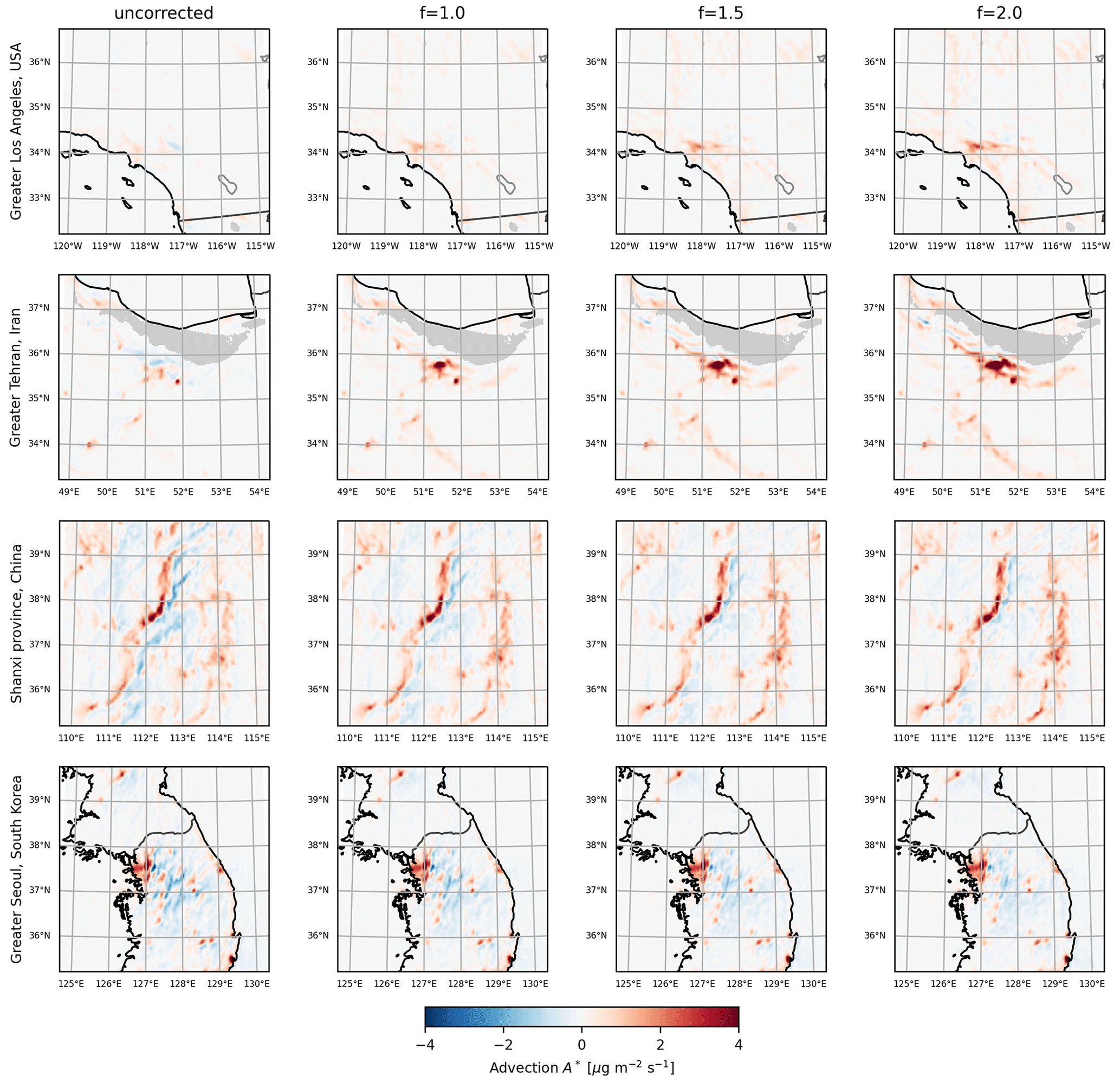
Figure A1Uncorrected and corrected advection maps for different scaling factors f of the topographic correction for Los Angeles, Tehran, the Shanxi province, and Seoul.
For the cities Los Angeles and Tehran, both exposed to high levels of NOx pollution and both close to high mountains, the topographic correction has a tremendous effect; Tehran, almost invisible in the uncorrected advection, becomes the place with the highest advection worldwide (i.e., candidate no. 0, classified as area source) after applying the topographic correction.
For northern China and South Korea, the uncorrected advection shows strong dipolar patterns of positive and negative advection values. These patterns caused several local maxima to be classified as “negative” in v1 of the catalog (Beirle et al., 2021). By applying the topographic correction, these patterns are suppressed, allowing for the identification of several additional point sources. However, even for f = 2 (corresponding to a NOx scale height of 500 m), the dipolar patterns do not vanish completely. On the other hand, a high value of f introduces new artifacts afar from the sources, for instance north of Los Angeles or south of Tehran. This can be understood since here the NOx scale height is larger, and the appropriate f would be lower.
Without additional knowledge about the (location-dependent) NOx scale height, the application of the topographic correction term is thus a compromise. For v2 of the catalog, we choose a value of f = 1.5, corresponding to a net NOx scale height of 667 m. For the error estimate, a relative uncertainty of 33 % (corresponding to f in the range of 1.0–2.0, or NOx scale height in the range 500–1000 m) is assumed for the topographic correction term.
Consider a point source with NOx emissions E. Following the emission plume in a Lagrangian reference frame, the amount of NOx as a function of time is proportional to for a first-order lifetime τ. Thus, also the chemical loss of NOx L decreases exponentially with time. Due to overall mass balance, L can be written as
since the integrated loss must equal the initial emissions E.
The integrated advection contains both emissions and losses, within 15 km. In order to receive the emissions, the contribution of the loss term has to be quantified and corrected for. For a given wind vector w, the spatial integration over 15 km radius can be transformed into a temporal integration over the residence time:
Without loss of generality, the spatial integration can be expressed in a coordinate system where x follows the wind direction. Thus, the integration in the across-wind direction y does not contribute to the chemical loss.
The spatial integration of the advection yields
with ∘ denoting the spatial integration over a circle with 15 km radius.
Therefore, the point source emissions can be derived by scaling the spatially integrated advection with the factor :
A former version of this article was published on 24 June 2021 and is available at https://doi.org/10.5194/essd-13-2995-2021.
The supplement related to this article is available online at: https://doi.org/10.5194/essd-15-3051-2023-supplement.
SB designed this study, performed the analysis, and wrote the paper with input from all co-authors. AJ and CB supported data processing. TW supervised the study.
The contact author has declared that none of the authors has any competing interests.
Publisher's note: Copernicus Publications remains neutral with regard to jurisdictional claims in published maps and institutional affiliations.
We thank ESA and the TROPOMI L1/L2 teams for realizing TROPOMI and providing NO2 tropospheric data. This study received funding from the ESA World Emission project (https://www.world-emission.com, last access: 27 June 2023), and the v2 catalog of NOx point source emissions is also included in the World Emission Portal.
This research has been supported by the European Space Agency under the World Emission project (contract no. 4000137291/22/I-EF).
The article processing charges for this open-access publication were covered by the Max Planck Society.
This paper was edited by Jing Wei and reviewed by three anonymous referees.
American Meteorological Society: “Advection”, Glossary of Meteorology, http://glossary.ametsoc.org/wiki/Advection (last access: 27 June 2023), 2012. a
Beirle, S., Boersma, K. F., Platt, U., Lawrence, M. G., and Wagner, T.: Megacity Emissions and Lifetimes of Nitrogen Oxides Probed from Space, Science, 333, 1737–1739, https://doi.org/10.1126/science.1207824, 2011.
Beirle, S., Borger, C., Dörner, S., Li, A., Hu, Z., Liu, F., Wang, Y., and Wagner, T.: Pinpointing nitrogen oxide emissions from space, Sci. Adv., 5, eaax9800, https://doi.org/10.1126/sciadv.aax9800, 2019. a, b, c, d, e, f, g, h, i, j, k
Beirle, S., Borger, C., Dörner, S., Eskes, H., Kumar, V., de Laat, A., and Wagner, T.: Quantification of NOx point sources from the TROPOspheric Monitoring Instrument (TROPOMI), World Data Center for Climate (WDCC) at DKRZ, https://doi.org/10.26050/WDCC/Quant_NOx_TROPOMI, 2020.
Beirle, S., Borger, C., Dörner, S., Eskes, H., Kumar, V., de Laat, A., and Wagner, T.: Catalog of NOx emissions from point sources as derived from the divergence of the NO2 flux for TROPOMI, Earth Syst. Sci. Data, 13, 2995–3012, https://doi.org/10.5194/essd-13-2995-2021, 2021. a, b, c, d, e, f, g, h, i, j, k, l, m, n, o, p, q, r
Beirle, S., Borger, C., Jost, A., and Wagner, T.: Catalog of NOx point source emissions (version 2), World Data Center for Climate (WDCC) at DKRZ [data set], https://doi.org/10.26050/WDCC/No_xPointEmissionsV2, 2023. a, b, c
Brunner, D., Kuhlmann, G., Marshall, J., Clément, V., Fuhrer, O., Broquet, G., Löscher, A., and Meijer, Y.: Accounting for the vertical distribution of emissions in atmospheric CO2 simulations, Atmos. Chem. Phys., 19, 4541–4559, https://doi.org/10.5194/acp-19-4541-2019, 2019. a
Byers, L., Friedrich, J., Hennig, R., Kressig, A., Li, X., McCormick, C., and Malaguzzi Valeri, L.: A Global Database of Power Plants, World Resources Institute, Washington, DC, https://datasets.wri.org/dataset/globalpowerplantdatabase (last access: 27 June 2023), 2019. a
Compernolle, S., Argyrouli, A., Lutz, R., Sneep, M., Lambert, J.-C., Fjæraa, A. M., Hubert, D., Keppens, A., Loyola, D., O'Connor, E., Romahn, F., Stammes, P., Verhoelst, T., and Wang, P.: Validation of the Sentinel-5 Precursor TROPOMI cloud data with Cloudnet, Aura OMI O2–O2, MODIS, and Suomi-NPP VIIRS, Atmos. Meas. Tech., 14, 2451–2476, https://doi.org/10.5194/amt-14-2451-2021, 2021. a
de Foy, B. and Schauer, J.: An improved understanding of NOx emissions in South Asian megacities using TROPOMI NO2 retrievals, Environ. Res. Lett., 17, 024006, https://doi.org/10.1088/1748-9326/ac48b4, 2022. a, b
Dickerson, R. R., Stedman, D. H., and Delany, A. C.: Direct Measurements of ozone and Nitrogen Dioxide Photolysis Rates in the Troposphere, J. Geophys. Res., 87, 4933–4946, https://doi.org/10.1029/JC087iC07p04933, 1982. a
eGRID: Emissions & Generation Resource Integrated Database, United States Environmental Protection Agency (EPA), Washington, DC: Office of Atmospheric Programs, Clean Air Markets Division, https://www.epa.gov/egrid (last access: 27 June 2023), 2022. a
Eskes, H. J. and Boersma, K. F.: Averaging kernels for DOAS total-column satellite retrievals, Atmos. Chem. Phys., 3, 1285–1291, https://doi.org/10.5194/acp-3-1285-2003, 2003. a, b
Eskes, H., van Geffen, J., Sneep, M., Veefkind, P., Niemeijer, S., and Zehner, C.: S5P Nitrogen Dioxide v02.03.01 intermediate reprocessing on the S5P-PAL system: Readme file, https://data-portal.s5p-pal.com/product-docs/no2/PAL_reprocessing_NO2_v02.03.01_20211215.pdf (last access: 27 June 2023), 2021. a, b
Goldberg, D. L., Lu, Z., Streets, D. G., de Foy, B., Griffin, D., McLinden, C. A., Lamsal, L. N., Krotkov, N. A., and Eskes, H.: Enhanced Capabilities of TROPOMI NO2: Estimating NOx from North American Cities and Power Plants, Environ. Sci. Technol., 53, 12594–12601, https://doi.org/10.1021/acs.est.9b04488, 2019. a
Hersbach, H., Bell, B., Berrisford, P., Hirahara, S., Horányi, A., Muñoz-Sabater, J., Nicolas, J., Peubey, C., Radu, R., Schepers, D., Simmons, A., Soci, C., Abdalla, S., Abellan, X., Balsamo, G., Bechtold, P., Biavati, G., Bidlot, J., Bonavita, M., Chiara, G. D., Dahlgren, P., Dee, D., Diamantakis, M., Dragani, R., Flemming, J., Forbes, R., Fuentes, M., Geer, A., Haimberger, L., Healy, S., Hogan, R. J., Hólm, E., Janisková, M., Keeley, S., Laloyaux, P., Lopez, P., Lupu, C., Radnoti, G., Rosnay, P., de Rozum, I., Vamborg, F., Villaume, S., and Thépaut, J.-N.: The ERA5 global reanalysis, Q. J. Roy. Meteor. Soc., 146, 1999–2049, https://doi.org/10.1002/qj.3803, 2020. a
IUPAC Task Group on Atmospheric Chemical Kinetic Data Evaluation, Data Sheet NOx24, https://iupac.aeris-data.fr/catalogue/#/catalogue/categories/NOx (last access: 27 June 2023), 2013. a
Janssen, L. H. J. M., Van Wakeren, J. H. A., Van Duuren, H., and Elshout, A. J.: A classification of NO oxidation rates in power plant plumes based on atmospheric conditions, Atmos. Environ., 22, 43–53, https://doi.org/10.1016/0004-6981(88)90298-3, 1988. a, b, c
Jöckel, P., Kerkweg, A., Pozzer, A., Sander, R., Tost, H., Riede, H., Baumgaertner, A., Gromov, S., and Kern, B.: Development cycle 2 of the Modular Earth Submodel System (MESSy2), Geosci. Model Dev., 3, 717–752, https://doi.org/10.5194/gmd-3-717-2010, 2010. a
Jöckel, P., Tost, H., Pozzer, A., Kunze, M., Kirner, O., Brenninkmeijer, C. A. M., Brinkop, S., Cai, D. S., Dyroff, C., Eckstein, J., Frank, F., Garny, H., Gottschaldt, K.-D., Graf, P., Grewe, V., Kerkweg, A., Kern, B., Matthes, S., Mertens, M., Meul, S., Neumaier, M., Nützel, M., Oberländer-Hayn, S., Ruhnke, R., Runde, T., Sander, R., Scharffe, D., and Zahn, A.: Earth System Chemistry integrated Modelling (ESCiMo) with the Modular Earth Submodel System (MESSy) version 2.51, Geosci. Model Dev., 9, 1153–1200, https://doi.org/10.5194/gmd-9-1153-2016, 2016. a
Kuhn, L., Kuhn, J., Wagner, T., and Platt, U.: The NO2 camera based on gas correlation spectroscopy, Atmos. Meas. Tech., 15, 1395–1414, https://doi.org/10.5194/amt-15-1395-2022, 2022. a
Lange, K., Richter, A., and Burrows, J. P.: Variability of nitrogen oxide emission fluxes and lifetimes estimated from Sentinel-5P TROPOMI observations, Atmos. Chem. Phys., 22, 2745–2767, https://doi.org/10.5194/acp-22-2745-2022, 2022. a, b, c, d
Laughner, J. L. and Cohen, R. C.: Direct observation of changing NOx lifetime in North American cities, Science, 366, 723–727, https://doi.org/10.1126/science.aax6832, 2019. a, b
Monks, P. S. and Beirle, S.: Applications of Satellite Observations of Tropospheric Composition, in The Remote Sensing of Tropospheric Composition from Space, edited by: Burrows, J. P., Borrell, P., Platt, U., Guzzi, R., Platt, U., and Lanzerotti, L. J., Springer Berlin Heidelberg, 365–449, https://link.springer.com/chapter/10.1007/978-3-642-14791-3_8 (last access: 27 June 2023), 2011. a
PRTR Germany: Pollutant Release and Transfer Register for Germany, Umweltbundesamt, https://thru.de/fileadmin/SITE_MASTER/content/Dokumente/Downloads/01_Topthemen/PRTR-Daten_2020/XLSX_PRTR-Export_GERMANY_2022-04-29.zip (last access: 27 June 2023), 2022. a
Sun, K.: Derivation of Emissions from Satellite-Observed Column Amounts and Its Application to TROPOMI NO2 and CO Observations, Geophys. Res. Letters, 49, e2022GL101102, https://doi.org/10.1029/2022GL101102, 2022. a, b, c, d, e, f
Tilstra, L. G.: TROPOMI ATBD of the directionally dependent surface Lambertian-equivalent reflectivity, KNMI Report S5P-KNMI-L3-0301-RP, 13 January, https://d37onar3vnbj2y.cloudfront.net/static/surface/albedo/documents/s5p_dler_atbd_v1.2.0_2022-01-13_signed.pdf (last access: 27 June 2023), 2022. a
Tilstra, L. G., Tuinder, O. N. E., Wang, P., and Stammes, P.: Directionally dependent Lambertian-equivalent reflectivity (DLER) of the Earth's surface measured by the GOME-2 satellite instruments, Atmos. Meas. Tech., 14, 4219–4238, https://doi.org/10.5194/amt-14-4219-2021, 2021. a
van Geffen, J. H. G. M., Eskes, H. J., Boersma, K. F., Maasakkers, J. D., and Veefkind, J. P.: TROPOMI ATBD of the total and tropospheric NO2 data products, S5P-KNMI-L2-0005-RP, Royal Netherlands Meteorological Institute, https://sentinel.esa.int/documents/247904/2476257/Sentinel-5P-TROPOMI-ATBD-NO2-data-products (last access: 27 June 2023), 2019. a, b, c
van Geffen, J., Eskes, H., Compernolle, S., Pinardi, G., Verhoelst, T., Lambert, J.-C., Sneep, M., ter Linden, M., Ludewig, A., Boersma, K. F., and Veefkind, J. P.: Sentinel-5P TROPOMI NO2 retrieval: impact of version v2.2 improvements and comparisons with OMI and ground-based data, Atmos. Meas. Tech., 15, 2037–2060, https://doi.org/10.5194/amt-15-2037-2022, 2022. a, b, c, d
Veefkind, J. P., Aben, I., McMullan, K., Förster, H., de Vries, J., Otter, G., Claas, J., Eskes, H. J., de Haan, J. F., Kleipool, Q., van Weele, M., Hasekamp, O., Hoogeveen, R., Landgraf, J., Snel, R., Tol, P., Ingmann, P., Voors, R., Kruizinga, B., Vink, R., Visser, H., and Levelt, P. F.: TROPOMI on the ESA Sentinel-5 Precursor: A GMES mission for global observations of the atmospheric composition for climate, air quality and ozone layer applications, Remote Sens. Environ., 120, 70–83, https://doi.org/10.1016/j.rse.2011.09.027, 2012. a
Wagner, T., Warnach, S., Beirle, S., Bobrowski, N., Jost, A., Puķīte, J., and Theys, N.: Investigation of three-dimensional radiative transfer effects for UV–Vis satellite and ground-based observations of volcanic plumes, Atmos. Meas. Tech., 16, 1609–1662, https://doi.org/10.5194/amt-16-1609-2023, 2023. a, b
World Emission, ESA project, https://www.world-emission.com/ (last access: 27 June 2023), 2022. a
- Abstract
- Introduction
- Datasets
- Methods
- Results
- Discussion
- Data availability
- Conclusions
- Appendix A: Topographic correction
- Appendix B: Lifetime correction
- Note on former version
- Author contributions
- Competing interests
- Disclaimer
- Acknowledgements
- Financial support
- Review statement
- References
- Supplement