Data rescue of historical wind observations in Sweden since the 1920s

Instrumental measurements of wind speed and direction from the 1920s to the 1940s from 13 stations in Sweden have been rescued and digitized, making 165 additional station years of wind data available through the Swedish Meteorological and Hydrological Institute's open data portal. These stations measured wind through different versions of cup-type anemometers and were mainly situated at lighthouses along the coasts and at airports. The work followed the protocol “Guidelines on Best Practices for Climate Data Rescue” of the World Meteorological Organization consisting of (i) designing a template for digitization, (ii) digitizing records in paper journals by a scanner, (iii) typing numbers of wind speed and direction data into the template, and (iv) performing quality control of the raw observation data. Along with the digitization of the wind observations, meta data from the stations were collected and compiled as support to the following quality control and homogenization of the wind data. The meta data mainly consist of changes in observer and a small number of changes in instrument types and positions. The rescue of these early wind observations can help improve our understanding of long-term wind changes and multidecadal variability (e.g. the “stilling” vs. “reversal” phenomena) but also to evaluate and assess climate simulations of the past. Digitized data can be accessed through the Swedish Meteorological and Hydrological Institute and the following Zenodo repository: https://doi.org/10.5281/zenodo.5850264 (Zhou et al., 2022).

1 Introduction

The ongoing climate change, described by the Intergovernmental Panel on Climate Change (IPCC) (IPCC, 2021), raises the question of if, how, and why the wind climate in the world is changing. Winds have a large impact on many parts of the society, economy, and environment (Rayner, 2007; Vicente-Serrano et al., 2018; Vose et al., 2014; Pörtner et al., 2022). Extreme winds can for example affect buildings, infrastructure, shipping (Pörtner et al., 2022), extreme cold outbreaks in winter (Zhou et al., 2021), and energy production (Pörtner et al., 2022; Castro et al., 2011). To reduce greenhouse gas emissions, there is an urgent need to transform the energy system to be more sustainable and robust, where renewable wind energy can be a part of the solution (Pörtner et al., 2022). Of the global electricity generation, wind energy made up 6.6 % in 2021 (https://www.iea.org, last access: 7 April 2023). The global annual net wind power generation was 1870 TWh in 2021 and has to reach 7900 TWh in 2030 to meet the Net Zero Emission by 2050 scenario (https://www.iea.org, last access: 7 April 2023). To secure future energy production for Sweden, it is important to know how the wind climate is changing when extreme weather events are estimated to possibly cause up to a 16 % drop in power supply reliability for Swedish cities in future scenarios (Perera et al., 2020).

To better understand how and why the wind climate is changing, we need to improve our limited knowledge of historical wind changes and multidecadal variability. A fundamental challenge lies in rescuing old climate observations from weather archives such as those at the National Weather Services and derive homogeneous and complete data series, as stated by the World Meteorological Organization (WMO) (WMO, 2016). The quality of the observations can be affected by measurement inconsistencies (Aguilar et al., 2003), changes in the surrounding environment (Dienst et al., 2017), changes of station position (Wan et al., 2010), and drifting anemometers (Azorin-Molina et al., 2018). At the Swedish Meteorological and Hydrological Institute (SMHI) most of the meteorological data are available digitally since the 1960s, but before that, only a minor part of the data are in digital form.

Prior studies have shown a global reduction in wind speed (termed “stilling”; Roderick et al., 2007) over land from the 1960s to the 1980s (McVicar et al., 2012; IPCC, 2021) and from around 2010 a “reversal” with increasing wind speed (Dunn et al., 2016; Azorin-Molina et al., 2017, 2018; Zeng et al., 2019). In Sweden, near-surface wind speed showed a statistically significant decreasing trend during 1956–2013 with a stronger reduction during 1979–2008 (Minola et al., 2016). But when each season is studied separately, a small non-significant wind speed increase was detected for winter during 1979–2008, which was partly driven by the increasing North Atlantic Oscillation (NAO) index during those decades (Minola et al., 2016). In a more recent study, Minola et al. (2021) found a break in the stilling around 2010 when analysing near-surface mean wind speed and gusts in Sweden for 1997–2019. The detected stilling reversal was to a large extent attributed to changes in the NAO. They also found a greater increase in wind gusts compared to the mean wind speed. Additionally, changes in surface roughness were also identified as another driver of wind variability in Sweden.

The IPCC Sixth Assessment Report (AR6) Working Group 1 (WGI) (IPCC, 2021) stated that the confidence in wind changes is “low” to “medium”, highlighting that there is still much to learn about wind changes and multidecadal variability in a warming climate. One of the limitations to study the stilling and reversal periods is due to the low availability of centennial wind series and inhomogeneities of observed wind speed records (IPCC, 2021). Before the 2010s there were not many studies dealing with quality control and homogenization of wind observations (Xu et al., 2006; Rayner, 2007; Wern and Bärring, 2009), but during the last decade, some publications have increased the knowledge in this research area (Wan et al., 2010; Azorin-Molina et al., 2014, 2019; Minola et al., 2016). Due to lack of data, earlier studies of wind conditions in Sweden could only evaluate trends and variability back to the 1960s, highlighting the need of extending the digitally available wind observations further back in time (Minola et al., 2016).

Still, a vast amount of meteorological observational data are only present as paper journals in archives and thus not easily accessible for scientists to study climate change. WMO (WMO, 2016) stated that rescuing (digitize data and store them in a database that is backed up) old climate data from weather archives and creating homogeneous and complete data sets is a fundamental challenge facing the climate research community. The rescue and digitization of observational data is identified as a crucial step in producing new and robust historical reanalyses (Brönnimann et al., 2018) and in better assessing and attributing wind changes. There are other ongoing data rescue initiatives focused on digitizing historical wind records from weather archives. The project at http://www.weatherrescue.org (last access: 7 April 2023) has used volunteer citizen scientists to digitize observations from the mid-1800s to the beginning of the 1900s at stations in Scotland and other locations in Europe (Hawkins et al., 2019).

SMHI holds valuable wind records only available in paper journals prior to the 1940s, as the digitization of climate series at SMHI systematically started only in the 1950s–1960s. To rescue historical wind observations in Sweden from the 1920s to 1940s, the project “Assessing centennial wind speed variability from a historical weather data rescue project in Sweden” (WINDGUST) was initiated, aimed at filling the gap of data prior to 1939 and temporal inhomogeneity of wind data sets in Sweden, with the ultimate goal of bringing more wind data into the hands of scientists who seek to improve the limited knowledge on the causes of wind variability and change including that of stilling and reversal as discussed in global climate science.

Here we focus the results, challenges, and lessons learned from the first part on data rescue of the WINDGUST project. Methods and results of the homogenization are presented by Zhou et al. (2022), and the evaluation and attribution of trends are presented by Minola et al. (2023).

Table 1 Technical specification of anemometer types. The higher mounting height interval marked with an ^* is for the anemometers mounted at lighthouses.

Figure 1 Sandström cup anemometer (Östman, 1928).

2 A brief history of Swedish wind observations

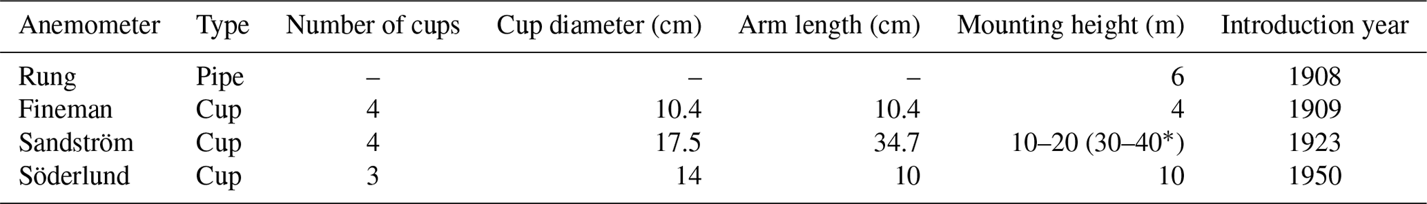
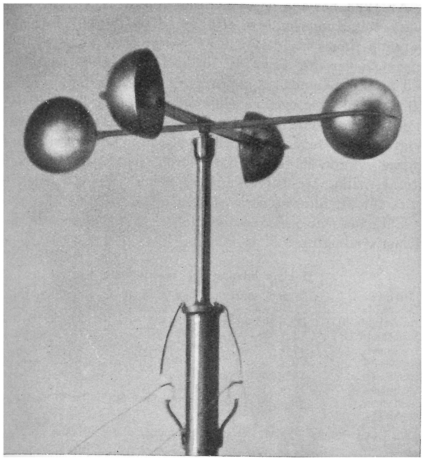
A Swedish national station network for meteorological ground-based observations was initiated by the Swedish Royal Academy of Science in 1858 (Östman, 1928). Meteorologiska Centralanstalten (MCA) (SMHI: https://www.smhi.se/, last access: 7 April 2023) was established in 1873 and was from then responsible for meteorological and hydrological observations across Sweden. Wind speed and direction have always been key weather observations. At the time of the initiation of the national station network in 1858, a wind speed scale from 0 to 4 was used. This scale was already introduced by Anders Celsius (1701–1744). In conjunction with the establishment of MCA in 1873, a 6-grade scale was taken into use. The six grades corresponded to every second grade in the 12-grade Beaufort scale. The complete 12-grade Beaufort scale was applied after the establishment of Statens Meteorologiska-Hydrologiska Anstalt (SMHA) in 1919 (SMHI; Sverker Hellström, personal communication, 2023). In the early years, wind observations were usually estimated using the scales mentioned above, although there were some instrumental measurements done already during the 20th century. From 1908 to 1910 around 15 lighthouse stations were equipped with Fineman anemometers and eight coastal stations with rung anemometers (Östman, 1928). The Fineman anemometer was a cup anemometer type, usually mounted on a 4 m high pole. To get the wind speed value, the observer had to climb up to the top of the pole. The rung anemometer was a tube with the wind blowing over a nozzle at the upper end of the tube. The wind created a pressure drop in the tube that moved a pointer, which showed the wind speed on a scale. The rung anemometers were mounted on 6 m high poles. In 1923, the Sandström cup-type anemometer (Fig. 1) was first introduced, and in 1928, this anemometer was in operation at around 30 coastal stations and 10 inland stations. This anemometer type had four cups and was installed in a mast 10–20 m aboveground or in a lighthouse tower that in some cases reaches 30–40 m above the ground. During the second half of the 20th century, wind measurements were performed with a Söderlund cup anemometer (Fig. 2) (SMHI; Sverker Hellström, personal communication, 2023) and since 1996 with a Thies ultrasonic anemometer at automatic weather stations (AWSs) (Wern and Bärring, 2009).

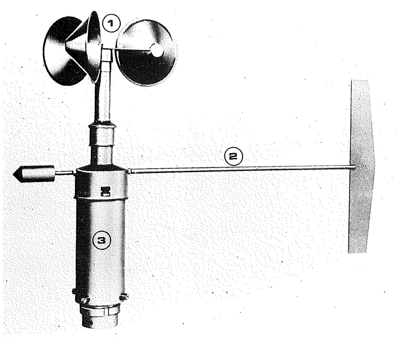
Figure 2 Söderlund cup anemometer used at SMHI observational station during the second half of the 20th century with cups (1), windvane (2), and transmission unit (3) (SMHI).

Figure 3 Sandström amemometer installations at four different Swedish stations in 1928. From left to right: Agö (mast), Grimskär (lighthouse), Ölands södra udde (lighthouse), and Lilljungfrun (storm warning mast) (Östman, 1928).

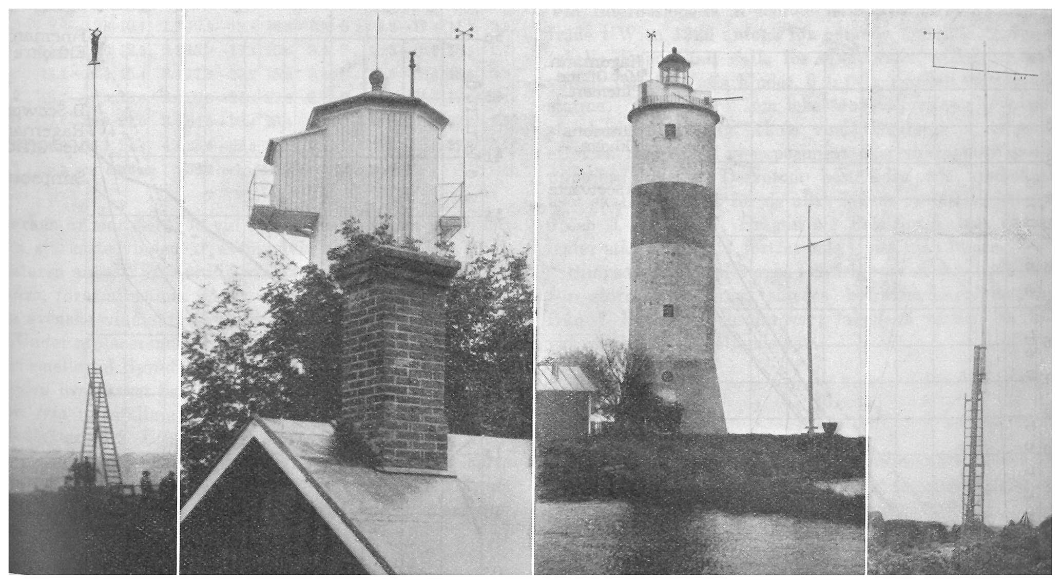
The early stations equipped with the above-described wind instruments (Table 1) were often lighthouses and airports (Fig. 3). The observations were done by the weather observers at these stations along with their primary duties as lighthouse keepers or airport crew. The observations were done at least 3 times a day and often 4 times a day: morning (08:00), midday (14:00), and evening (21:00) (Swedish normal time) before 1941. Between 1941 and 1946 the observations were done at 8:00, 14:00, and 19:00. From 1947 and onwards the hours were at 7:00, 13:00, and 19:00.

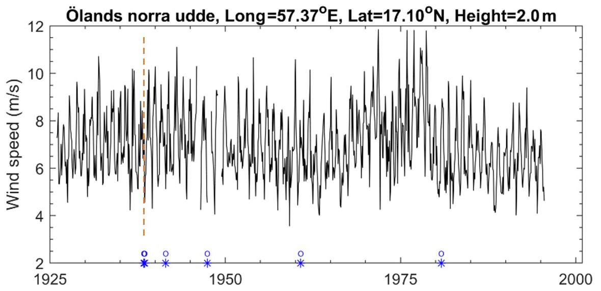
Figure 4 Wind speed observations at the station at Ölands norra udde from 1926 to 1996. Change of observer is marked in the lower part of the figure by a blue circle and star. A change of anemometer in 1938 is marked with a vertical dashed orange line (SMHI).

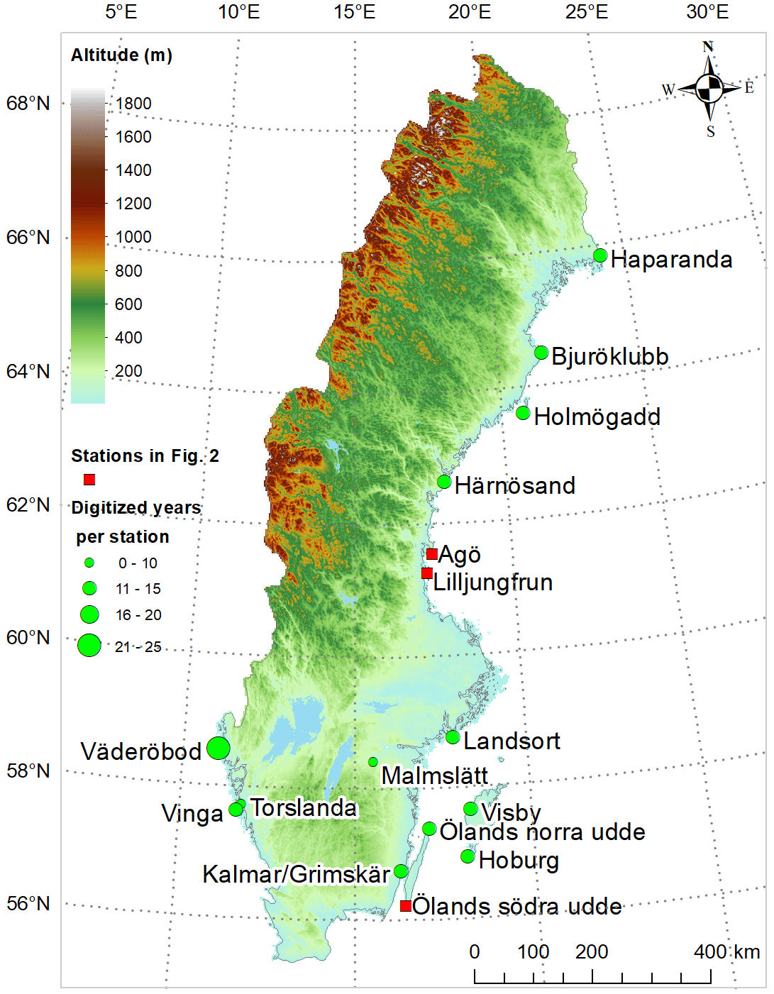
Figure 5 Elevation map of Sweden with the position of the wind stations that were digitized in green dots. Red squares show positions of the stations in the photographs in Fig. 2 (note that observations from these have not been digitized here, except Kalmar and Grimskär that were digitized) (SMHI).

As an example, at the station Ölands norra udde, the Sandström anemometer was installed in 1924 and then changed in 1938 to an SMHA no. 18 anemometer. In Fig. 4 wind speed observations are plotted, and the change of anemometer is marked by a vertical orange dashed line in the plot.

Table 2 The identification number (ID), position of the stations, and start and stop years of the digitized data and for the stations.

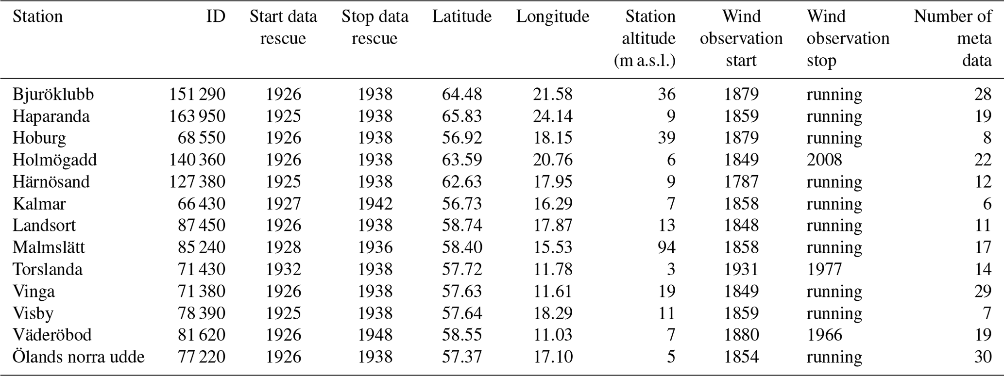
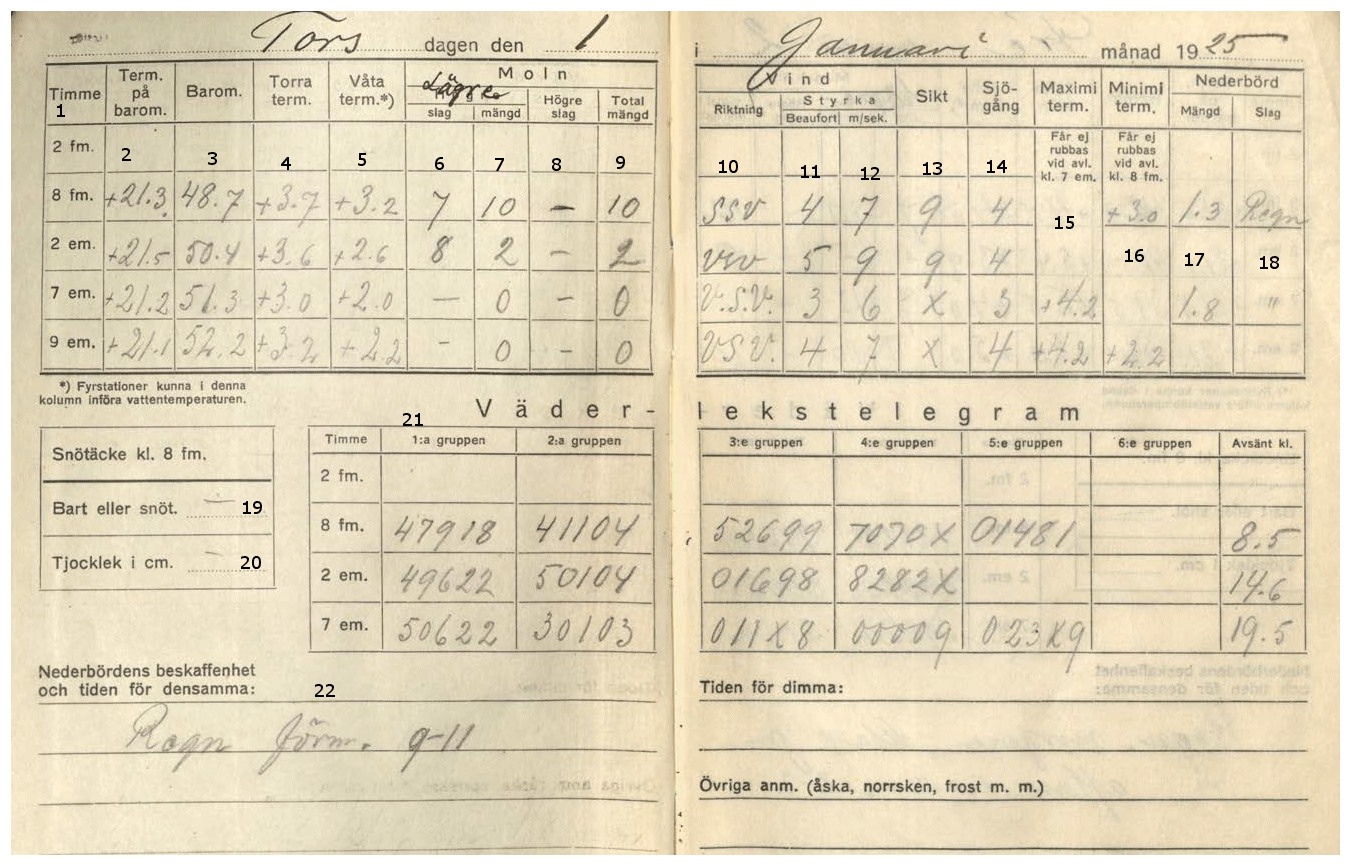
Figure 6 Paper journal for the Visby station, 1 January 1925. The columns are from left to right as follows: time of day (1), indoor temperature for correcting the mercury barometer reading (^∘C) (2), air pressure (mm hg, −700 units) (3), dry temperature (^∘C) (4), wet temperature (^∘C) (5), lower-cloud type (6), lower-cloud amount/cover (tenths) (7), higher-cloud type (8), total cloud amount/cover (tenths) (9), wind direction (10), wind speed (Beaufort) (11), wind speed (m s⁻¹) (12), visibility (code number) (13), sea waves (14), maximum temperature (^∘C) (15), minimum temperature (^∘C) (16), precipitation amount (mm) (17), and precipitation type (18). In the lower part of the page are boxes for snow cover: B (bare ground), S (snow cover), SB (mostly snow cover), and BS (mostly bare ground) (19), as well as depth (cm) (20) (to the left) and present weather codes (21) (middle and right). At the bottom of the page are lines for extra notes concerning the type and time for precipitation, mist, and other observations such as thunder, aurora borealis, and frost (22) (SMHI).

3 Rescue of historical wind data

The WINDGUST project rescued historical wind observations available in the old weather journals at the SMHI archives for the 1920s–1940s by applying the well-defined protocol “Guidelines on Best Practices for Climate Data Rescue” of WMO (WMO, 2016). The process consisted of (i) designing a template for digitization, (ii) digitizing paper journals by an imaging process based on scanning or photographs, (iii) typing numbers of wind speed data into the template, and (iv) performing a quality control of the data digitized in (iii). Prior studies have concluded that manual typing is the quickest and most reliable data rescue method compared to other methods such as speech recognition and optical character recognition (Brönnimann et al., 2006; Ashcroft et al., 2018).

First, an inventory of suitable and available observations in Sweden on wind speed and direction was performed in the archives of SMHI. Only stations with wind speed data in metres per second (m s⁻¹) were selected. These stations were considered to have been equipped with anemometers so the wind speed could be expected to have been measured. At stations where wind speed was only reported in the Beaufort scale, the wind speed was expected to have been estimated from signs in the surrounding environment due to the fact that information from the journals and the wind series were discarded for digitization. This resulted in a list of 13 stations across Sweden (Fig. 5 and Table 2). The stations were located in different parts of the country, mostly along the coast. Although it was not a criterion for selection, 10 of the stations are still active, making analyses over a full century possible. The archive sheets did contain other variables that will be digitized according to the priority of stations and variables in coming years.

3.1 Weather data in paper journals

The paper journals for the selected stations were brought from the archive at SMHI. The journals used were books, each covering 6 months of data. Each book lookup represented observations for 1 d (Fig. 6). The observations were done 3 to 4 times a day (see Sect. 2)

Figure 7 Bookeye 4 scanning equipment used at SMHI (SMHI).

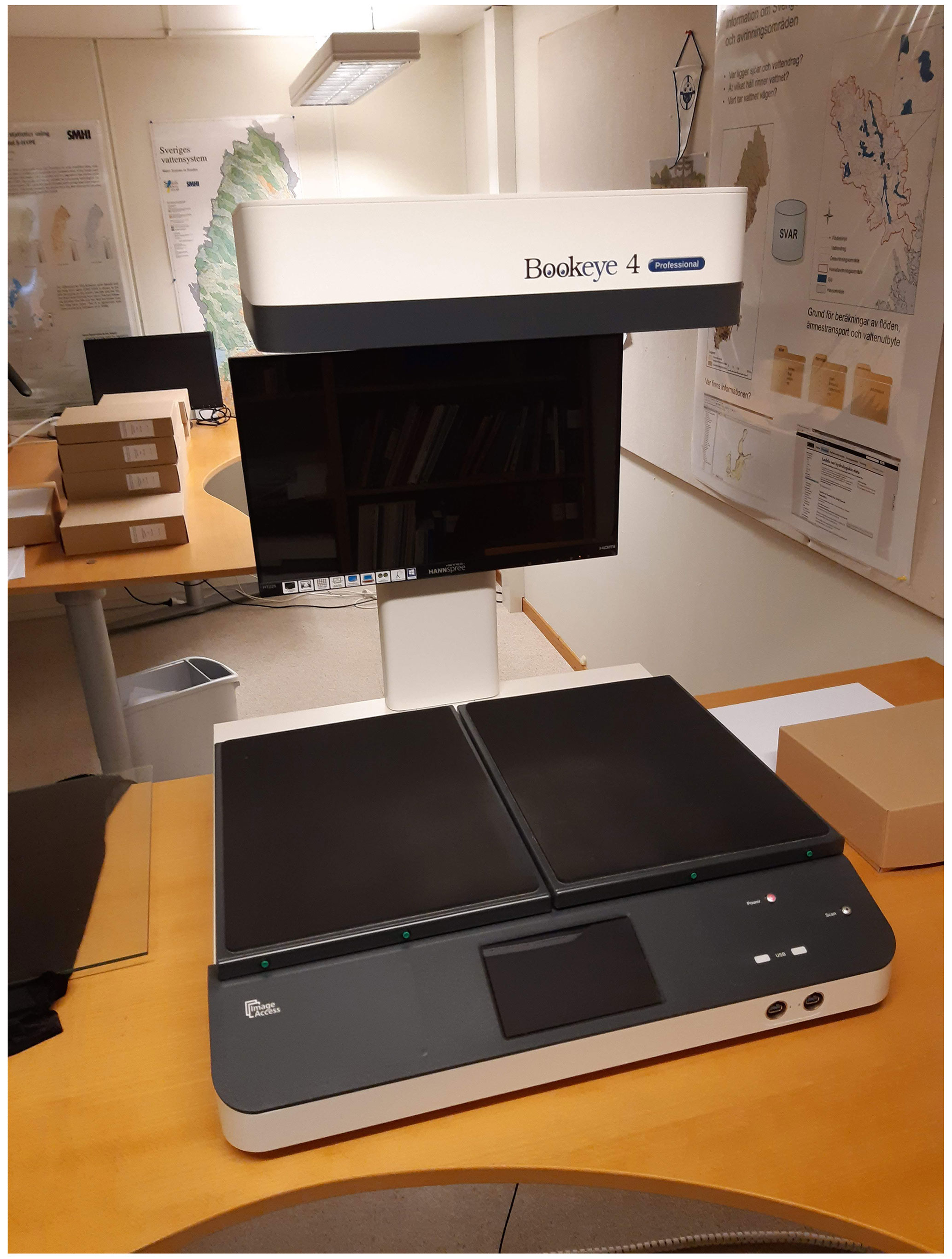
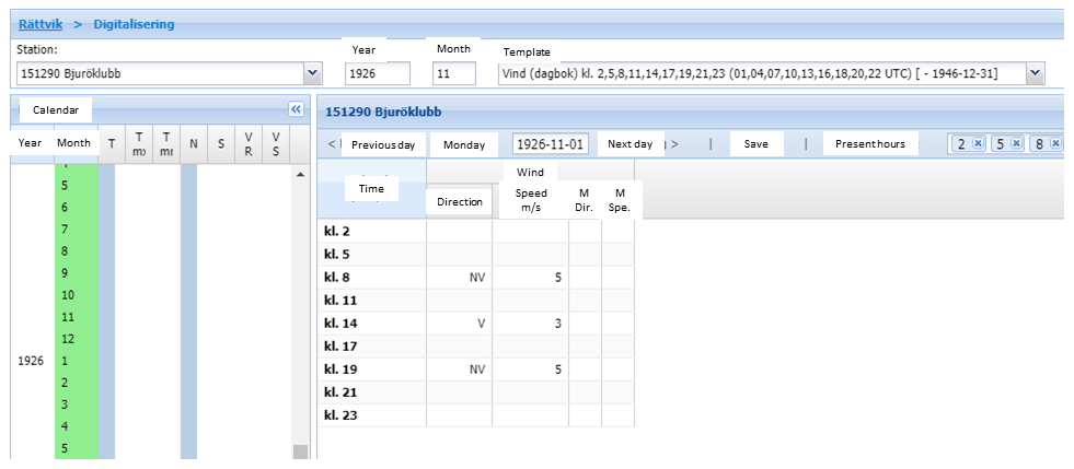
Figure 8 Digitization template for the data rescue of wind observations at SMHI (SMHI).

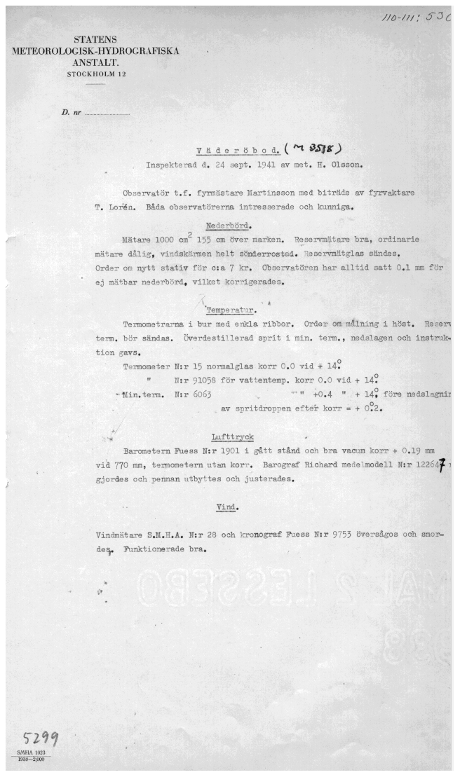
Figure 9 Meta data of the station Väderöbod from 24 September 1941. The lowest section with the title “Vind” concerns wind measurements (SMHI).

3.2 Scanning

Each book lookup was scanned in a dedicated Bookeye 4 scanner (Fig. 7). Each image of a book lookup was compiled to a pdf file containing 1 year of observations. The scanner could be operated both by hand using buttons or a computer mouse or by foot using a pedal. The scanning had to be done in the institute, as the original journals were not allowed to leave the building. The paper journals were mostly in good shape and were handled with care. In a few cases, however, data were missing in the paper journals or the handwriting was difficult to read.

3.3 Digitization

A template for the digitization was designed and then used in the project (Fig. 8). The scanned image of the paper journal was viewed on one computer screen, and the values from the paper journals were typed into the template on another computer screen. When the values were typed into the template, they were automatically stored in the observational MORA (Meteorologiska observationer för realtid och arkiv) database at SMHI. The scanning and digitization were static work, and the staff performing these duties were encouraged to often take short breaks to not get stuck in one working position for too long.

3.4 Quality control

Once the wind measurements were stored in the observational MORA database at SMHI, a first quality-control check was performed to detect missing or suspicious data. If data gaps were found, the reason for missing data was investigated. High-wind speeds were also checked. For instance, logical tests were performed where the maximum wind speed could not be lower than the minimum wind speed. All wind speed values higher than the known record for each station were also checked. Further details of these tests are discussed in Sect. 4.3.

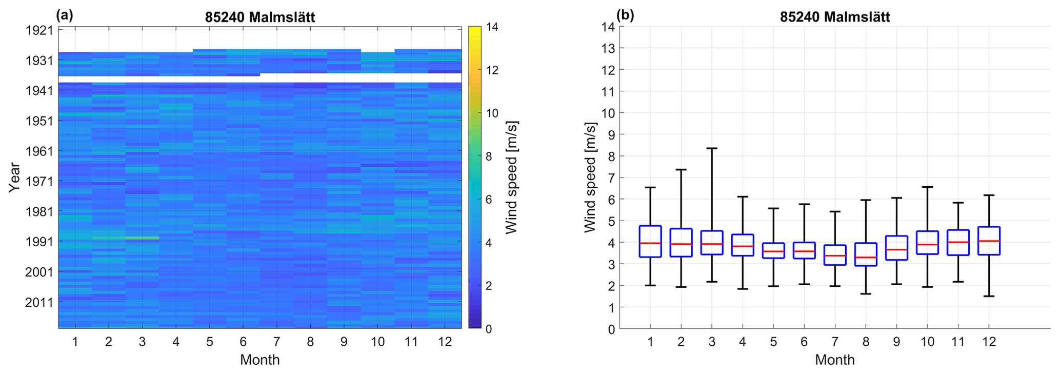
Figure 10 Data screening plot for Malmslätt as a typical inland station. (a) The data coverage and the monthly mean wind speed value according to the colour bar. (b) The monthly wind speed, where the red line is the monthly mean wind speed, the upper and lower limits of the blue box are the 75 and 25th percentiles, and the end bars represent the maximum and minimum monthly mean wind speed (SMHI).

3.5 Meta data

Meta data for all digitized stations were compiled in the project. The information was gathered from the protocols of the inspection of the stations done by the SMHI staff. Every station was inspected with intervals from every year to every fifth year, and any changes at the stations were noted. Changes could be in the surroundings such as new buildings or old buildings that had been removed, trees or bushes that had grown up or been removed, new observers, or in instrumentation or routines. If routines decided by SMHI were not followed, it was corrected. A shortcoming of the protocols is that if a change is noted, the exact date of the change is seldom known. The change then occurred sometime between the present inspection and the prior inspection, which could mean a time span of 1 to 5 years. The lowest section in Fig. 9 is an example of meta data from the station Väderöbod from 24 September 1941. Translated to English, the text is “Wind. Wind instrument S.M.H.A. No. 28 and chronograph Fuess No. 9753 were inspected and lubricated. Good functionality.”. The meta data were compiled in digital files with codes attributed to different types of changes, which made it possible to read the meta data files automatically with computer scripts as a part of the homogenization method.

3.6 MORA database

The digitized wind observations were directly stored in the observational MORA database at SMHI. In MORA, meteorological observations are stored, both as a digital historical archive ranging from the oldest observations of temperature from Uppsala in 1722 to the new real-time observations. The database also contains some statistics such as mean values for month, year, and 30-year periods. The database contains more than 19 billion values from around 4300 Swedish stations, 16 000 international stations, and over 100 meteorological parameters. Swedish observational data can be accessed by anyone manually through web interfaces or by an application programming interface (API) also called machine-to-machine interfaces. Most of the meteorological observations in Sweden from 1960 onwards are digitally available in MORA and can be accessed through SMHI's open data portal: https://www.smhi.se/data (last access: 7 April 2023). However, the observations before 1960 are only partly available in MORA, as the digitization of these data is still ongoing.

4 Results

The work, completed by four SMHI staff members during 2200 man hours, was finished in the spring of 2021. They had then scanned and digitized 13 selected stations spanning the years 1925 to 1948.

4.1 Data screening

A data screening was performed for the 13 stations that were digitized to visualize the data coverage, monthly variability, and wind speed range. The stations were classified into two groups, coastal and inland stations. Malmslätt (Fig. 10) represents a typical inland station with the highest monthly mean wind speed during October to March around 4 m s⁻¹. The maximum monthly mean was reported for March (8–9 m s⁻¹). For all months the lowest monthly means are about 2 m s⁻¹. Observations have been continuously registered at Malmslätt since 1945. Before that, storing of journals were more random, which caused the data gap from July 1936 to January 1939.

Figure 11 Data screening plot for Vinga as a typical coastal station. (a) The data coverage and the monthly mean wind speed value according to the colour bar. (b) The monthly wind speed, where the red line is the monthly mean wind speed, the upper and lower limits of the box are the 75 and 25th percentiles, and the end bars represent the maximum and minimum monthly mean wind speed (SMHI).

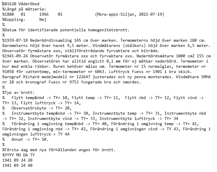
Figure 12 Example of the file format for a compiled station meta data file. The example shows extracted information for Väderöbod. The names of the observers are replaced with “xxx” due to General Data Protection Regulation (GDPR) rules (SMHI).

Vinga (Fig. 11) represents a coastal station with the highest monthly mean wind speed generally during November and December ranging between 8 and 9 m s⁻¹. The lowest mean monthly wind speed, 5–6 m s⁻¹, is obtained in May. The maximum monthly mean wind speed is approximately 13 m s⁻¹ in November and minimum around 3 m s⁻¹ in August. The data gap in the 1940s was due to observations that by mistake were not digitized in the project but will be digitized after the project. To fill the data gap between 1997 and 2007, the nearby station Trubaduren is suggested to be used in a future project. Kalmar, Härnösand, and Haparanda show monthly wind speed patterns typical for inland stations, even though the stations are located close to the sea. In Kalmar the station was located on a small island, and in Härnösand and Haparanda the stations were located around 1 km from the coast. The inland character of the station can be explained by the fact that coastal stations on the Swedish east coast are somewhat shielded for the dominating westerly to the south-westerly winds and possibly some additional obstacles in the station vicinity, such as buildings or trees. For all three stations and most particularly for Haparanda, located in the far north of Bay of Bothnia, sea ice cover can give those stations more of an inland character in some winters. Screening plots for all digitized stations can be found in Appendix A.

4.2 Meta data compilation

Meta data for all digitized stations were compiled into digital files with the file format shown in Fig. 12. The format of the meta data files enabled the files to be read by a computer programme, which some of the homogenization methods have functionality for. First, the data files contain a station identification number, name of the station, as well as a start and stop year for the series. After that follows a free text section summarizing identified potential homogeneity breaks. Then, a section explaining the meaning of the break-type codes. Last in the files, there is a list of identified break dates and types. For the 13 digitized stations, 122 potential homogeneity breaks were identified in the meta data, with a mean value of 17 per station. The number of potential breaks per station ranged from 6 to 30.

4.3 Quality control

The digitized values were checked for errors as soon as possible in parallel to the continuous digitization to be able to correct unclear instructions and improve the process. Suspicious values were flagged and checked an extra time in the paper journals. Several quality-control checks were performed as described in Sect. 3.4. The following is a list of examples of problems found and how they were dealt with:

• Sometimes the wind observation was digitized at an erroneous time of day in the database. This was discovered when the digitized data were controlled and the observations were not stored with the correct observational time in the database. This could be corrected by running a programming script.

• For some stations, identical values had been digitized at two consecutive time stamps. Again, the paper journals were consulted, and the value at the incorrect time was corrected.

• On some occasions, the wrong column from the paper journals had been digitized, such as visibility data instead of wind speed. The missing wind data were digitized to replace the incorrect values.

• A large number of gaps in the digitized data were identified. This was found to be the times marked as calm weather (no wind) that the staff performing the digitization had left empty in the digitized files due to unclear instructions. These gaps were filled in with zeros for wind speed and wind direction.

• On some occasions there was no wind speed noted in metres per second (m s⁻¹) in the paper journals but only wind speed in Beaufort. If the gap in metres per second was only one single observation time, the value in metres per second was interpolated from the Beaufort value. If the gap was several observational times, values in metres per second were not interpolated but marked as missing data.

• Some dates (pages) were found missing in the electronic image files from the scanning. The wind speed values for the missing dates (pages) were digitized after the scanning process.

• A number of the highest wind speed values for each station were checked against the paper journals an extra time, and some values were found to be wrong and were corrected.

The performed quality control is, however, not complete. When starting to analyse data in more detail, additional suspicious values will probably appear. Then there is a possibility to check the original value in the scanned paper journal. If the value in the database turns out to be wrong then the database can be updated with the correct value, and the quality of the analysis will improve. During the time period of digitization of 1920 to 1940, totally, 242 364 values were digitized. Out of these 242 364 values, 392 values were corrected during the QC. For the 10 stations with century-long records, the ratio of missing monthly values from 1920 to now was 9 %, 975 out of 11 222 values.

5 Homogenization

The homogenization was performed and described by Zhou et al. (2022). The penalized maximal F test (PMF) method was used and a combination of CERA-20C and ERA5 was used as a reference data set for the homogenization. For the 13 stations, 71 change points were detected. Most change points were found in the years 1935–1944, 1956–1964, and around 1985. Around 38 % of the detected change points were confirmed by meta data from the stations. To adjust the time series for the detected change point, a mean-matching adjustment was applied using up to 5 years of data before and after each change point. The most recent segment was chosen as reference. The 13 homogenized wind speed time series showed an increase of 0.09 m s⁻¹ per decade that peaked around 1990. From 1990 to 2005 a decrease by 25 % in the trend followed. After 2005 the homogenized time series showed a rapid recovery in wind speed.

6 Attribution of trends

Further analysis of the wind speed trends over Sweden showed a stilling during 1926–1960, a stabilization from 1960 to 1990 and then a second stilling during 1990–2003 (Minola et al., 2023). A slight recovery was found during 2003–2014. Three reanalysis data sets were used to attribute the trends found over Sweden to large-scale atmospheric circulation patterns (e.g. the North Atlantic Oscillation). The three reanalysis data sets were ERA20C, ERA5, and NOAA-CIRES. The analysis showed that changes in large-scale atmospheric circulations mainly drive the observed low-frequency variability of near-surface wind speed but could not fully represent the periods of strong stilling over Sweden for which other factors are needed for attribution (e.g. changes in surface roughness).

7 Discussion

The scanning of the original journals enables an additional electronic backup of the data and improves the accessibility when the electronic files can be sent to external users while the original journals have to be kept in the archive. The electronic copies also made it possible to perform the digitization at any place suitable for the staff doing the digitization. It would be beneficial if the work can continue with digitization of more stations further back in time. This work provides a significant addition to the available wind observations for Sweden, but 13 stations are far from enough to be representative for the whole country of Sweden. One possibility could be to digitize wind speed observations recorded with the different observed wind scales previously used, which would demand a profound quality evaluation to determine their usability.

This work contributes to satisfy the need to increase the amount of digitized wind observations available for the international research community, as stated by WMO (2016). The digitized observations enable additional insight into the historical variability and trends of the wind climate in Sweden. There is still a vast amount of meteorological data that are only stored in paper journals that need to be digitized to be rescued for future generations and made practically accessible and usable for fellow researchers. This urges the national meteorological services to continue their efforts to rescue and digitize meteorological data. In this project we acknowledge the benefit of having experienced digitization staff that work in close collaboration with climate experts to identify and correct errors in the digitization. The International Data Rescue (I-DARE; https://www.idare-portal.org; last access: 7 April 2023) portal collects and provides information on a large number of data rescue activities and facilitates sharing of experience and methods in this field. Some projects have successfully tried to engage the public in citizen science contributions where people could volunteer to digitize data from scanned historical records (Hawkins et al., 2019; Craig and Hawkins, 2020) using the web service of http://www.weatherrescue.org (last access: 7 April 2023), where the quality control was conducted by triple parallel digitization of three independent persons. To further accelerate the pace in rescuing and digitization of historical data the techniques of artificial intelligence (AI), machine learning (ML), and optical character recognition (OCR) could be developed and applied in this field as discussed by Campbell et al. (2021). These techniques have so far been of limited value due to the low ratio of accuracy, but the methods are improving fast. In the near future, there will probably be a growing number of successful projects rescuing data by these and similar methods.

At SMHI the work continues to rescue and digitize historical meteorological, hydrological, and oceanographic observations from the archives of paper journals spanning over more than 150 years, and the methods discussed above are developed to facilitate and speed up this work further.

8 Data availability

Digitized data can be accessed through the SMHI open data portal and the Zenodo repository: https://doi.org/10.5281/zenodo.5850264 (Zhou et al., 2022).

9 Conclusions

With the newly digitized observations, studies of wind conditions in Sweden could be extended to the time period from around 1920 to present, enveloping one full century of wind measurements. The results of this work were fruitfully brought forward by Zhou et al. (2022) who homogenized and investigated the historical variability and trends in surface wind speed in Sweden for the last century and Minola et al. (2023) who investigated the causes of the detected trends in the Swedish wind climate. Digitized data can be accessed through the SMHI open data portal and the Zenodo repository: https://doi.org/10.5281/zenodo.5850264 (Zhou et al., 2022).

Appendix A: Data screening figures

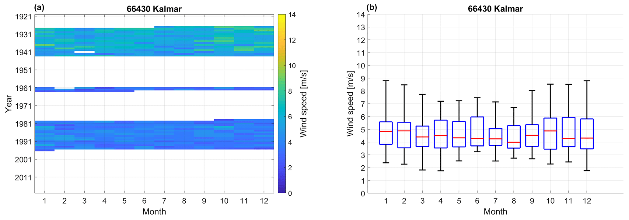
Figure A1 Data screening plot for Kalmar. (a) The data coverage and the monthly mean wind speed value according to the colour bar. (b) The monthly wind speed, where the red line is the monthly mean wind speed, the upper and lower limits of the blue box are the 75 and 25th percentiles, and the end bars represent the maximum and minimum monthly mean wind speed.

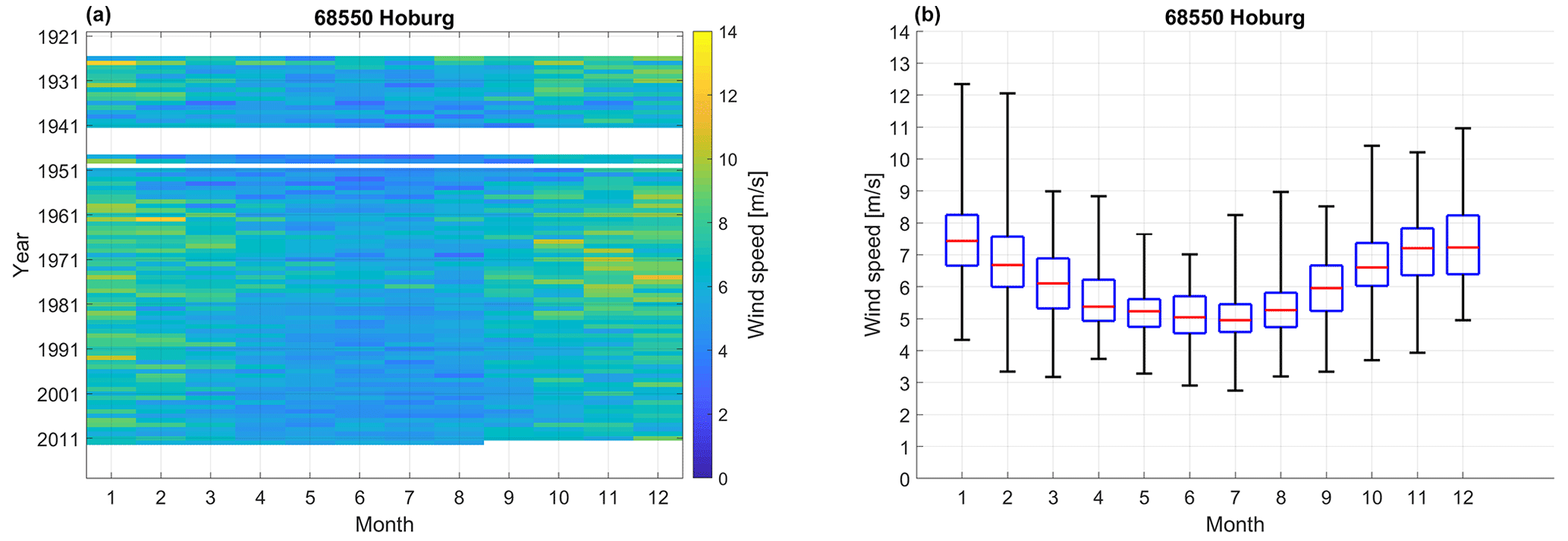
Figure A2 Data screening plot for Hoburg. (a) The data coverage and the monthly mean wind speed value according to the colour bar. (b) The monthly wind speed, where the red line is the monthly mean wind speed, the upper and lower limits of the blue box are the 75 and 25th percentiles, and the end bars represent the maximum and minimum monthly mean wind speed.

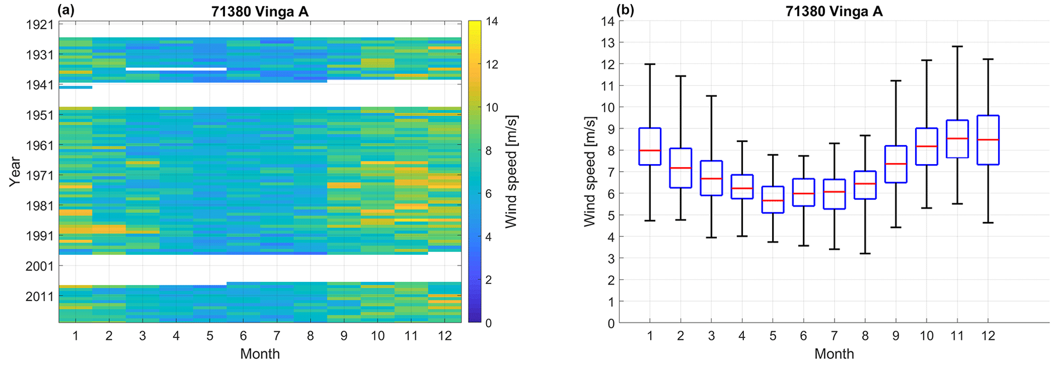
Figure A3 Data screening plot for Vinga. (a) The data coverage and the monthly mean wind speed value according to the colour bar. (b) The monthly wind speed, where the red line is the monthly mean wind speed, the upper and lower limits of the blue box are the 75 and 25th percentiles, and the end bars represent the maximum and minimum monthly mean wind speed.

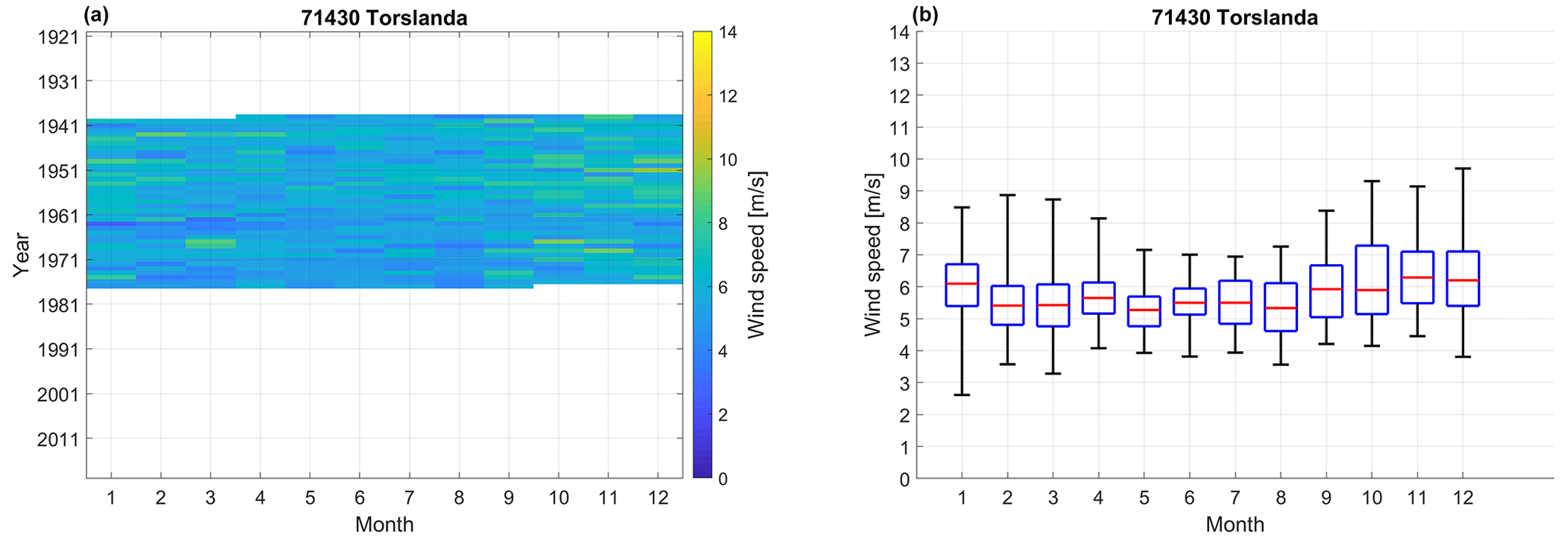
Figure A4 Data screening plot for Torslanda. (a) The data coverage and the monthly mean wind speed value according to the colour bar. (b) The monthly wind speed, where the red line is the monthly mean wind speed, the upper and lower limits of the blue box are the 75 and 25th percentiles, and the end bars represent the maximum and minimum monthly mean wind speed.

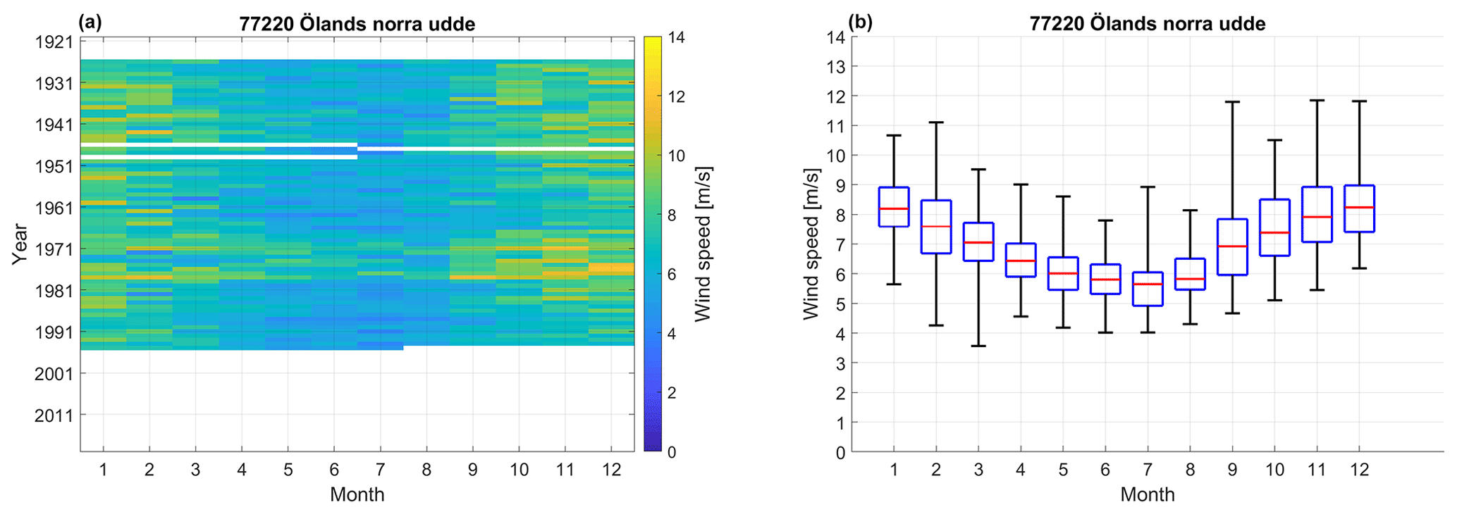
Figure A5 Data screening plot for Ölands norra udde. (a) The data coverage and the monthly mean wind speed value according to the colour bar. (b) The monthly wind speed, where the red line is the monthly mean wind speed, the upper and lower limits of the blue box are the 75 and 25th percentiles, and the end bars represent the maximum and minimum monthly mean wind speed.

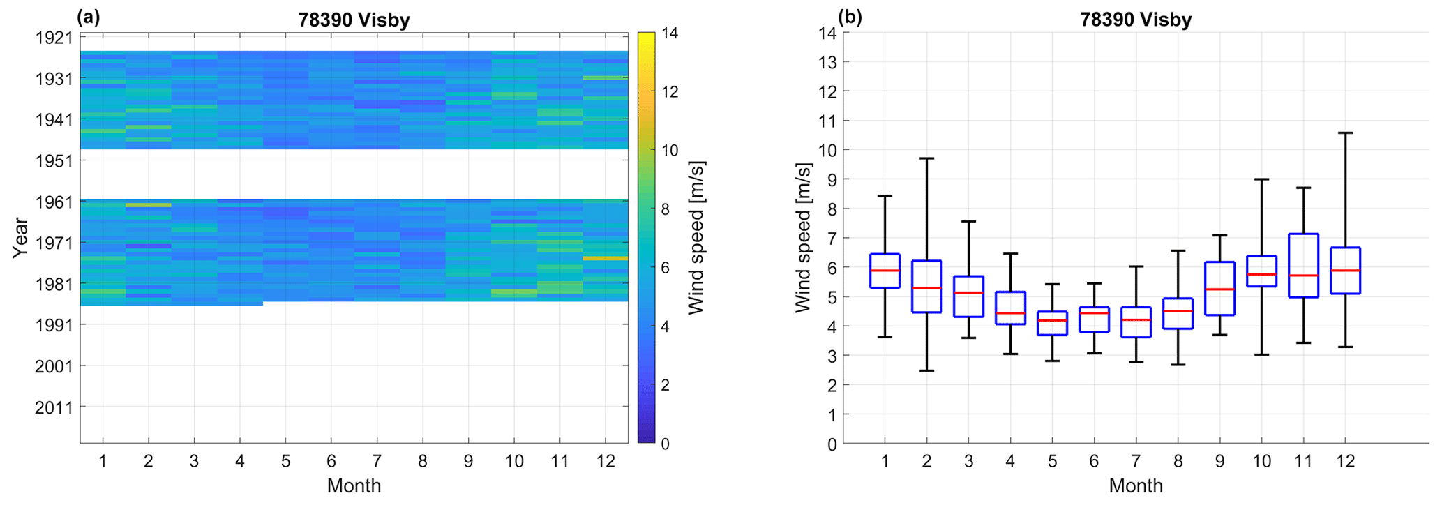
Figure A6 Data screening plot for Visby. (a) The data coverage and the monthly mean wind speed value according to the colour bar. (b) The monthly wind speed, where the red line is the monthly mean wind speed, the upper and lower limits of the blue box are the 75 and 25th percentiles, and the end bars represent the maximum and minimum monthly mean wind speed.

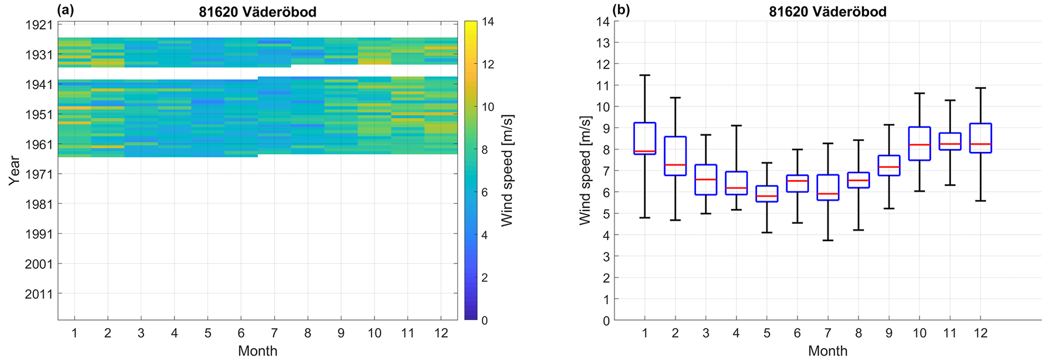
Figure A7 Data screening plot for Väderöbod. (a) The data coverage and the monthly mean wind speed value according to the colour bar. (b) The monthly wind speed, where the red line is the monthly mean wind speed, the upper and lower limits of the blue box are the 75 and 25th percentiles, and the end bars represent the maximum and minimum monthly mean wind speed.

Figure A8 Data screening plot for Malmslätt. (a) The data coverage and the monthly mean wind speed value according to the colour bar. (b) The monthly wind speed, where the red line is the monthly mean wind speed, the upper and lower limits of the blue box are the 75 and 25th percentiles, and the end bars represent the maximum and minimum monthly mean wind speed.

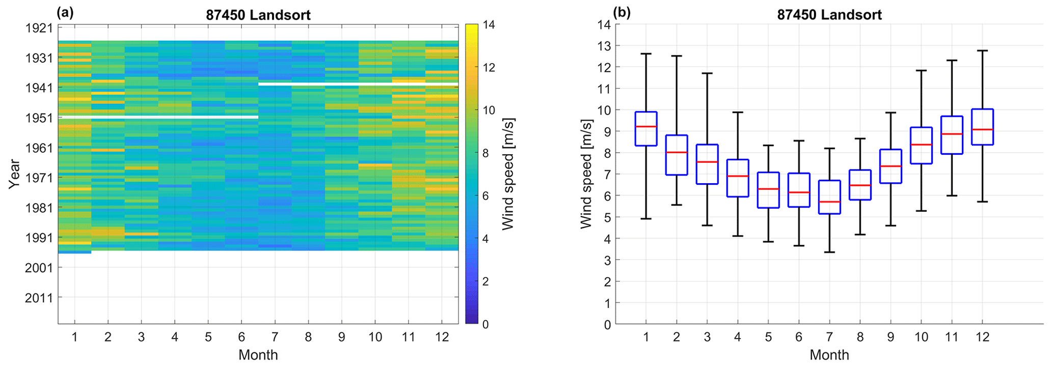
Figure A9 Data screening plot for Landsort. (a) The data coverage and the monthly mean wind speed value according to the colour bar. (b) The monthly wind speed, where the red line is the monthly mean wind speed, the upper and lower limits of the blue box are the 75 and 25th percentiles, and the end bars represent the maximum and minimum monthly mean wind speed.

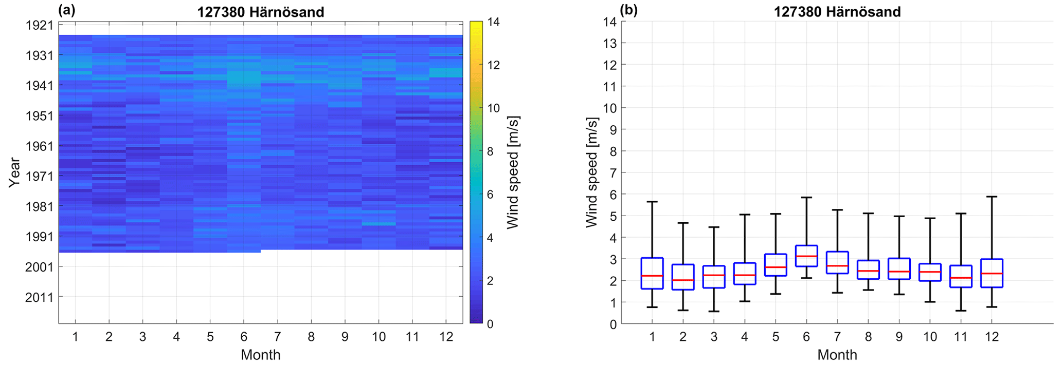
Figure A10 Data screening plot for Härnösand. (a) The data coverage and the monthly mean wind speed value according to the colour bar. (b) The monthly wind speed, where the red line is the monthly mean wind speed, the upper and lower limits of the blue box are the 75 and 25th percentiles, and the end bars represent the maximum and minimum monthly mean wind speed.

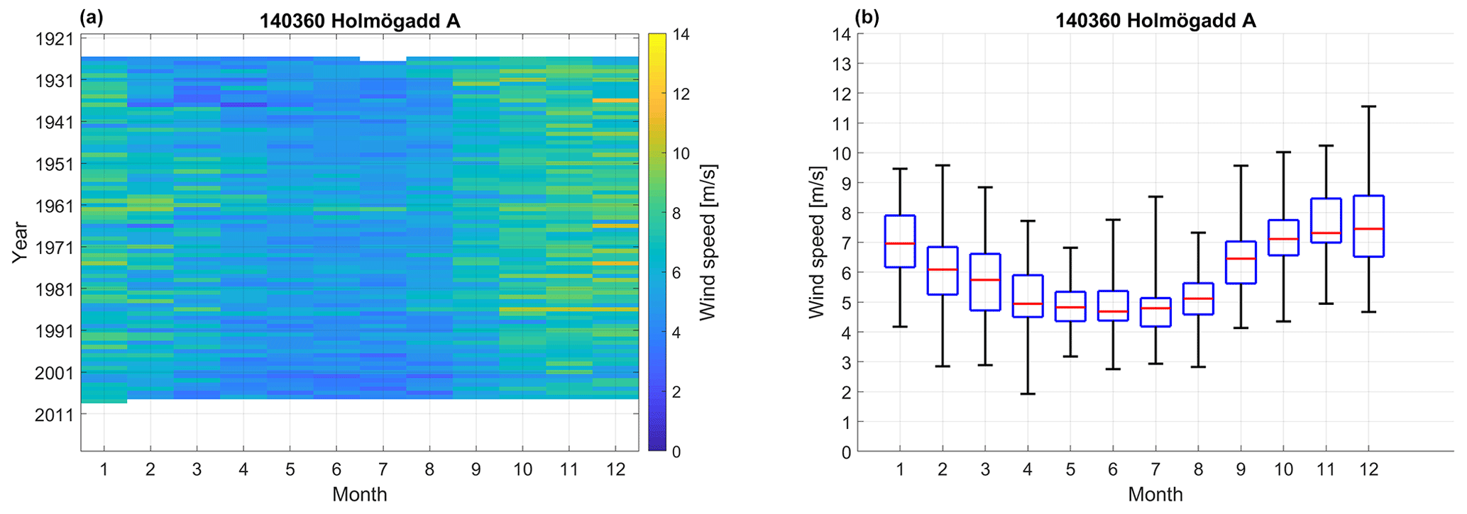
Figure A11 Data screening plot for Holmögadd. (a) The data coverage and the monthly mean wind speed value according to the colour bar. (b) The monthly wind speed, where the red line is the monthly mean wind speed, the upper and lower limits of the blue box are the 75 and 25th percentiles, and the end bars represent the maximum and minimum monthly mean wind speed.

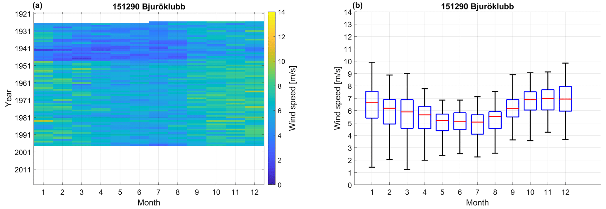
Figure A12 Data screening plot for Bjuröklubb. (a) The data coverage and the monthly mean wind speed value according to the colour bar. (b) The monthly wind speed, where the red line is the monthly mean wind speed, the upper and lower limits of the blue box are the 75 and 25th percentiles, and the end bars represent the maximum and minimum monthly mean wind speed.

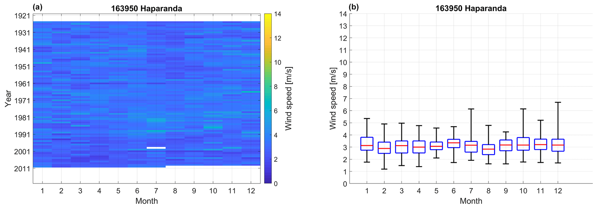
Figure A13 Data screening plot for Haparanda. (a) The data coverage and the monthly mean wind speed value according to the colour bar. (b) The monthly wind speed, where the red line is the monthly mean wind speed, the upper and lower limits of the blue box are the 75 and 25th percentiles, and the end bars represent the maximum and minimum monthly mean wind speed.