the Creative Commons Attribution 4.0 License.
the Creative Commons Attribution 4.0 License.
 | 27 Apr 2023
A remote-sensing-based dataset to characterize the ecosystem functioning and functional diversity in the Biosphere Reserve of the Sierra Nevada (southeastern Spain)
Javier Cabello
Andrés Reyes
Emilio Guirado
Julio Peñas
Antonio J. Pérez-Luque
Domingo Alcaraz-Segura
Conservation biology faces the challenge of safeguarding the ecosystem functions and ecological processes (the water cycle, nutrients, energy flow, and community dynamics) that sustain the multiple facets of biodiversity. Characterization and evaluation of these processes and functions can be carried out through functional attributes or traits related to the exchanges of matter and energy between vegetation and the atmosphere. Based on this principle, satellite imagery can provide integrative spatiotemporal characterizations of ecosystem functions at local to global scales. Here, we provide a multitemporal dataset at protected-area level that characterizes the spatial patterns and temporal dynamics of ecosystem functioning in the Biosphere Reserve of the Sierra Nevada (Spain), captured through the spectral Enhanced Vegetation Index (EVI, using product MOD13Q1.006 from the MODIS sensor) from 2001 to 2018. The database contains, at the annual scale, a synthetic map of Ecosystem Functional Type (EFT) classes from three Ecosystem Functional Attributes (EFAs): (i) descriptors of annual primary production, (ii) seasonality, and (iii) phenology of carbon gains. It also includes two ecosystem functional-diversity indices derived from the above datasets: (i) EFT richness and (ii) EFT rarity. Finally, it provides interannual summaries for all previously mentioned variables, i.e., their long-term means and interannual variability. The datasets are available at two open-source sites (PANGAEA: https://doi.org/10.1594/PANGAEA.924792; Cazorla et al., 2020a; interannual summaries at http://obsnev.es/apps/efts_SN.html, last access: 17 April 2023). This dataset provides scientists, environmental managers, and the public in general with valuable information on the first characterization of ecosystem functional diversity based on primary production developed in the Sierra Nevada, a biodiversity hotspot in the Mediterranean basin and an exceptional natural laboratory for ecological research within the Long-Term Social-Ecological Research (LTER) network.
- Article
(8231 KB) - Full-text XML
-
Supplement
(743 KB) - BibTeX
- EndNote


A better characterization of the functional dimension of biodiversity is required to develop management approaches that ensure nature contributions to human well-being (Jax, 2010; Cabello et al., 2012a; Bennet et al., 2015). A set of essential variables for characterizing and monitoring ecosystem functioning is necessary to achieve this goal (Pereira et al., 2013). Such variables are critical to understanding the dynamics of ecological systems (Petchey and Gaston, 2006), the links between biological diversity and ecosystem services (Balvanera et al., 2006; Haines-Young and Potschin, 2010), and the mechanisms of ecological resilience (Mouchet et al., 2010). In addition, there have been calls for the use of ecosystem functioning variables to assess functional diversity at large scales to measure biosphere integrity (Mace et al., 2014; Steffen et al., 2015), one of the most challenging planetary boundaries to assess (Steffen et al., 2015). Despite the importance of ecosystem functioning variables and the conceptual frameworks developed to promote their use (Pettorelli et al., 2018), they have seldom been incorporated into ecosystem monitoring (see Alcaraz-Segura et al., 2009; Fernández et al., 2010; Cabello et al., 2016; Skidmore et al., 2021).
Characterization and evaluation of ecosystem functioning can be carried out by monitoring functional traits or attributes related to the matter and energy exchanges between biota and the atmosphere (Box et al., 1989; Running et al., 2000). Nowadays, the use of satellite imagery provides useful methods to derive such attributes, allowing for the spatially explicit characterization of ecosystem functioning and its heterogeneity (i.e., functional diversity) from local (Fernández et al., 2010), regional (Alcaraz-Segura et al., 2006, 2013), and global scales (Ivits et al., 2013; Skidmore et al., 2021). Theoretical and empirical models enable essential functional variables of ecosystems such as primary production, evapotranspiration, surface temperature, or albedo to be estimated based on spectral indices derived from satellite images (e.g., the Enhanced Vegetation Index; EVI) (Pettorelli et al., 2005; Fernández et al., 2010; Lee et al., 2013). Among them, primary production is one of the most integrative and essential descriptors of ecosystem functioning (Virginia et al., 2001; Pereira et al., 2013) since it has a significant role in the carbon cycle (i.e., the energy input to the trophic web and the driving force behind many ecological processes) (Xiao et al., 2019). Moreover, primary production provides a holistic response to environmental changes and constitutes a synthetic indicator of ecosystem health (Costanza et al., 1992; Skidmore et al., 2015).
To characterize ecosystem functioning focusing on primary production, we can use the satellite-derived approach based on Ecosystem Functional Types (EFTs), defined as patches of the land surface that share similar dynamics in the matter and energy exchanges between the biota and the physical environment (Paruelo et al., 2001; Alcaraz-Segura et al., 2006). EFTs are derived from three Ecosystem Functional Attributes (EFAs) that describe the seasonal dynamics of carbon gains through time series of spectral vegetation indices: (1) EVI annual mean (a surrogate of annual primary production), (2) EVI annual standard deviation (a descriptor of seasonality or the differences between the growing and non-growing seasons), and (3) the annual date of the maximum EVI (a phenological indicator of the date within a year on which the growing period is centered). Biologically, these three metrics can be interpreted as surrogates of the total amount and timing of primary production (Paruelo et al., 2001; Pettorelli et al., 2005; Alcaraz-Segura et al., 2006), one of the most integrative indicators of ecosystem functioning (Virginia et al., 2001). Since the EFT concept appeared in 2001 (Paruelo et al., 2001), its applicability has grown to characterize functional heterogeneity from local to global scales (Alcaraz-Segura et al., 2006, 2013; Karlsen et al., 2006; Duro et al., 2007; Fernández et al., 2010; Geerken, 2009; Ivits et al., 2013; Cabello et al., 2013; Pérez-Hoyos et al., 2014; Müller et al., 2014; Wang and Huang, 2015; Villarreal et al., 2018; Coops et al., 2018; Mucina, 2019; Cazorla et al., 2020b).
Here, we present a dataset that describes the spatial heterogeneity and temporal variability of a key measure of ecosystem functioning and ecosystem functional-diversity patterns in the Sierra Nevada Biosphere Reserve, a protected area in southeastern Spain (Fig. 1). We derived the dataset from the analysis of the intra-annual and interannual variation of vegetation greenness captured through the EVI spectral vegetation index, as a surrogate of primary production, during the 2001–2018 period. First, for each year, we provide maps of three EFAs: (i) annual primary production and (ii) seasonality and (iii) phenology of carbon gains as well as their integration into a synthetic mapping of EFTs as discrete landscape functional units. Second, based on these units, we present two functional-diversity metrics: EFT richness and EFT rarity. Finally, by considering the yearly maps, we calculated interannual summaries, i.e., interannual means and interannual variability, to show the average conditions and the stability of the ecosystem functioning of the period (the workflow is provided in Fig. 2). The abundance of long-term datasets from multiple disciplines in the Sierra Nevada constitutes an opportunity to explore the role of ecosystem functioning and functional diversity in ecohydrological and species distribution modeling, climate-change mitigation and adaptation, ecological resilience, adaptive management, and mountain ecosystem service supply, since humankind depends on freshwater of mountain regions, which are hotspots of biodiversity and a key destination for recreation activities (Grêt-Regamey et al., 2012).
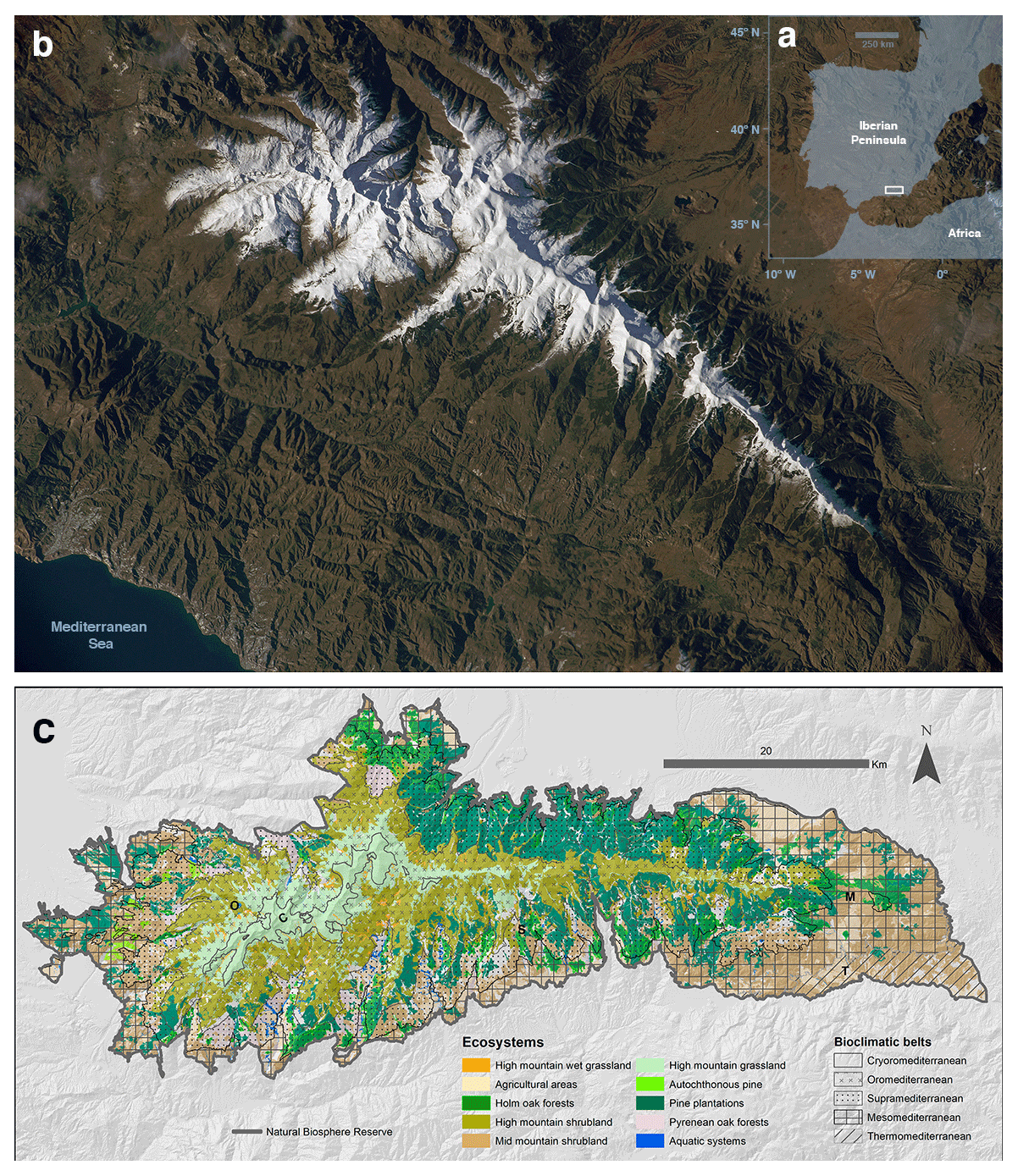
Figure 1Study area: Sierra Nevada Biosphere Reserve. (a) Location in the context of the Iberian Peninsula; (b) remote view of the Sierra Nevada region (image from the International Space Station taken in December 2014, courtesy of the Earth Science and Remote Sensing Unit, 615 NASA Johnson Space Center); (c) delimitation of the Biosphere Reserve and the distribution of the main ecosystems (Pérez-Luque et al., 2019) and thermotype bioclimatic belts (Molero and Marfil, 2015).
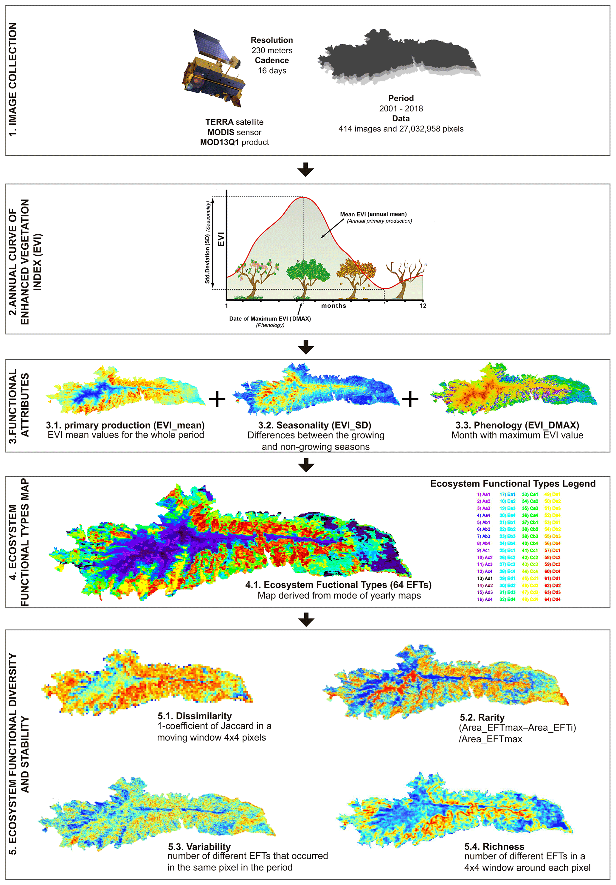
Figure 2Workflow to characterize the ecosystem functioning and functional diversity of the Sierra Nevada. The MODIS sensor product MOD13Q1 on board NASA's Terra satellite was used. This product contains maximum-value composite images with 16 d temporal resolution (23 images per year) and 232 m spatial resolution for the Enhanced Vegetation Index (EVI) (1). The study period was from 2001 to 2018. Three Ecosystem Functional Attributes (EFAs) describing ecosystem functioning were calculated from the EVI seasonal curve for each year (2 and 3). The range of values for each attribute was divided into four intervals, resulting in a potential number of 64 Ecosystem Functional Types (EFTs; ) (4). From EFTs, we derived four metrics related to ecosystem functional diversity (i.e., EFT richness and rarity) and ecosystem functional stability (i.e., interannual variability and dissimilarity) (5).
2.1 Data acquisition and processing
We based ecosystem functioning characterization on analyzing the temporal dynamics of the EVI from 2001 to 2018. We chose the EVI instead of any other vegetation index (such as the SAVI, soil-adjusted vegetation index, ARVI, atmospherically resistant vegetation index, or NDVI, normalized difference vegetation index) as an indicator of carbon gains since it is more reliable in both low- and high-vegetation-cover situations (Huete et al., 1997). Furthermore, the EVI reduces the influence of atmospheric conditions on vegetation index values and corrects for canopy background signals.
The EVI is computed following this equation (Eq. 1):
NIR/RED/Blue are atmospherically corrected (Rayleigh and ozone-absorption) surface reflectances for near-infrared, red, and blue wavelengths, respectively. L is the canopy background adjustment that addresses the nonlinear and differential transfer through a canopy of the NIR and red radiations. C1 and C2 are the coefficients of the aerosol resistance term, which uses the blue band to correct for aerosol influences in the red band. The coefficients adopted in the MODIS–EVI algorithm are L=1, C1=6, C2=7.5, and G (gain factor) = 2.5. The EVI values range from −1 to +1, where negative values correspond to snow, ice, or water, and values closer to +1 represent a high density of green leaves (Huete et al., 2002).
We obtained the EVI from the MOD13Q1.006 product of the MODIS sensor on board NASA's Terra satellite (Didan et al., 2015). The MOD13Q1.006 EVI product is computed from atmospherically corrected bidirectional surface reflectance by choosing automatically the best-available pixel value from all the acquisitions (four per day) in a 16 d period based on quality, cloud presence, and viewing geometry (Huete et al., 1999; Didan et al., 2015). To further remove the potential remaining effect of snow, ice, and water in our dataset, we transformed negative EVI values into zeros. Thus, we obtained a maximum-value composite image every 16 d (23 images per year). Despite its moderate spatial resolution (232 m spatial resolution at the Equator), we chose the MOD13Q1.006 product as the basis for our data since it offers a long time series (almost 20 years) every 16 d, which allows for the characterization of the temporal dynamics of ecosystem functioning (Anderson, 2018).
MOD13Q1.006 images were available in Google Earth Engine (GEE) servers at https://developers.google.com/earth-engine/datasets/catalog/MODIS_006_MOD13Q1 (last access: 17 April 2023), where we processed them. GEE combines a multi-petabyte catalog of satellite imagery and geospatial datasets with planetary-scale analysis capabilities (Gorelick et al., 2017). We used the main Javascript programming interface to build the algorithms and requests to GEE servers. EVI values are multiplied by 10 000 to store them as real numbers to occupy less disk space (both in the original MOD13Q1.006 product and in our dataset).
2.2 Calculating EFAs
We calculated three EFA maps known to capture most of the variance of the seasonal curve or annual dynamics of vegetation indices (Paruelo et al., 2001; Alcaraz-Segura et al., 2006, 2009): the EVI annual mean (EVI_mean, an estimator of primary production), the EVI seasonal standard deviation (EVI_sSD, a descriptor of seasonality, i.e., the differences between the growing and non-growing seasons), and the date of the maximum EVI (EVI_DMAX, a phenological indicator of the month with the maximum EVI) (Fig. 3). To summarize the EFAs of the 2001–2018 period, we calculated the interannual mean for each attribute (using linear statistics for EVI_mean and EVI_sSD and circular statistics for EVI_DMAX).
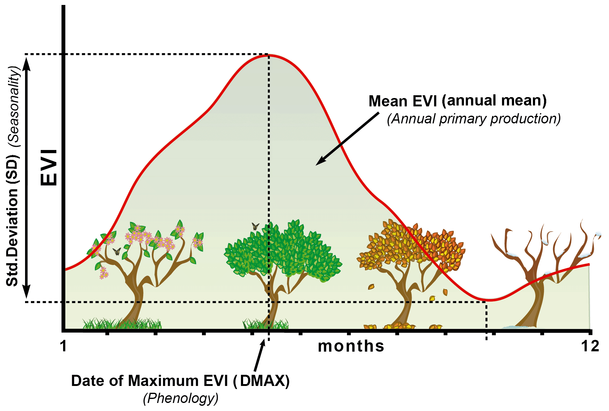
Figure 3Seasonal dynamics of the EVI and EVI-derived metrics or EFAs. The x axis corresponds to the months of the year and the y axis to the EVI values. EFAs were the annual mean of the EVI, an estimator of annual primary production (EVI_mean), the EVI seasonal coefficient of variation, i.e., a descriptor of seasonality or the differences between the growing and non-growing seasons (EVI_sSD), and the date of the maximum EVI, a phenological indicator of the growing season (EVI_DMAX). We chose these three EVI metrics or EFAs since they capture most of the variance (96.5 %) of the EVI seasonal dynamics in a principal component analysis.
To explore the robustness of these metrics in our study area, we examined their correlation with the first axes of a principal component analysis (PCA) run on the EVI annual curve of the average year (i.e., 12 EVI values corresponding to the interannual means of the 18 (1 per year) maximum EVI values of each month. These three metrics were highly correlated with the first two PCA axes (which accumulated 96.5 % of the variance), as previously reported for many regions (Townshend et al., 1985; Paruelo and Lauenroth, 1995; Paruelo et al., 2001; Alcaraz-Segura et al., 2006, 2009; Ivits et al., 2013). This component of the analysis is presented in full in Supplement A.
2.3 Identifying EFTs
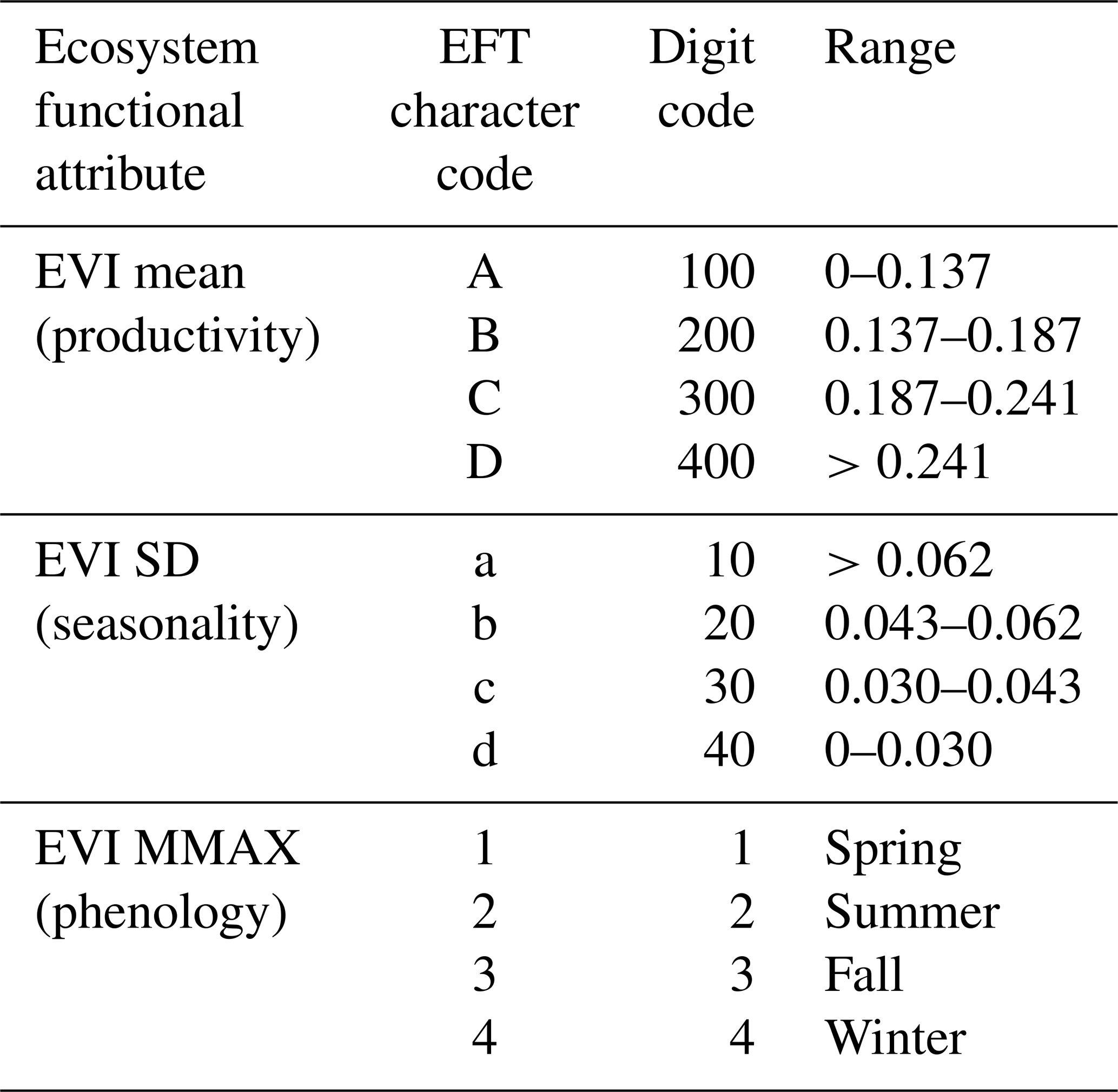
EFTs were identified by dividing the EFAs into four intervals and combining them into a potential number of 64 EFT classes (), following a similar approach to Alcaraz-Segura et al. (2013) (Fig. 2). For EVI_DMAX, the four intervals agreed with the four seasons of the year: January to March: winter, April to June: spring, July to September: summer, and October to December: fall. For EVI_mean and EVI_sSD, we extracted the first, second, and third quartiles for each year. We verified that an 18-year period was long enough to stabilize the quartiles by running a sensitivity analysis (see Supplement B). Then, for each quartile, we calculated the interannual mean of the 18-year period and used them as breaks between classes (Supplement B, Table S4). These breaks were applied back to each year as the thresholds for EVI_Mean and EVI_sSD to set EFT classes (Table 1). Finally, to summarize the EFTs, we calculated the most-frequent EFT (i.e., the EFT mode for each pixel) of the 2001–2018 period. To name EFTs, we used two letters and a number: the first, capital, letter indicates primary production (EVI_mean), increasing from A to D; the second, lowercased, letter represents seasonality (EVI_sSD), decreasing from a to d; finally, the numbers are a phenological indicator of the growing season (EVI_DMAX), with values 1 – spring, 2 – summer, 3 – fall, and 4 – winter (Table 1). The EFT alphanumeric code (Aa1 to Dd4) corresponds to the numeric code (1 to 64) in the .TIF files, which is shown in the legend of Fig. 4d.
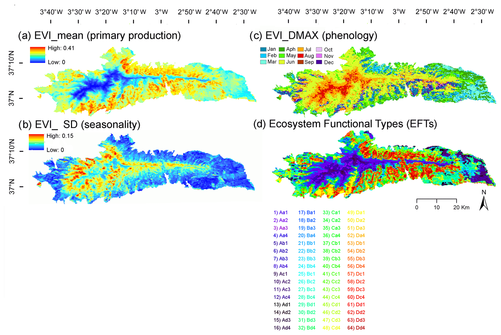
Figure 4EFAs (a–c) and EFTs (d) describing the functioning of the vegetation canopy based on the EVI, derived from MOD13Q1-TERRA (pixel 232 m) for the period 2001–2018. EFAs were (a–c) the annual mean of the EVI, an estimator of annual primary production (EVI_mean), the EVI seasonal coefficient of variation, i.e., a descriptor of seasonality or the differences between the growing and non-growing seasons (EVI_sSD), and the date of the maximum EVI, a phenological indicator of the growing season (EVI_DMAX). To name EFTs (d), we used two letters and a number: the first, capital, letter indicates primary production (EVI_mean), increasing from A to D, the second, lowercased, letter represents seasonality (EVI_sSD), decreasing from a to d, and finally, the numbers are a phenological indicator of the growing season (EVI_DMAX), with values 1 – spring, 2 – summer, 3 – fall, and 4 – winter (Table 1). The EFT alphanumeric code (Aa1 to Dd4) corresponds to the numeric code (1 to 64) in the .TIF files, as shown in the panel legend (d).
Table 1Ecosystem Functional Attribute (EFA) ranges used for the identification of Ecosystem Functional Types (EFTs) in the Sierra Nevada Biosphere Reserve. For EVI_DMAX, the four intervals agree with the four seasons of the year. For EVI_mean and EVI_sSD, we extracted the first, second, and third quartiles for each year and then calculated the interannual mean of each quartile (their average over the 18-year period). The values of both EVI_mean and EVI_sSD are multiplied by 10 000 in the .TIF files to save disk space.
2.4 Deriving ecosystem functional-diversity metrics
We derived two diversity metrics of ecosystem functional diversity from the EFT map: EFT richness and EFT rarity. EFT richness was calculated for each year by counting the number of different EFTs in a 4×4-pixel moving window around each pixel (top-left center pixel of a 4×4 kernel) (modified from Alcaraz-Segura et al., 2013). Each pixel received a richness value calculated by counting how many different EFTs there were in the 4×4-pixel search window. We chose a 4×4-pixel window because it offered the most acceptable spatial resolution without saturating the number of EFT classes per kernel (i.e., smaller kernel sizes resulted in a high proportion of moving windows saturated) (see the sensitivity analysis of kernel size in Sect. 3.2 and Supplement C).
We calculated EFT rarity as the extension of each EFT compared to the most-abundant EFT in the study area (Eq. 2) (Cabello et al., 2013). Then, the average rarity map of all the years was obtained.
where Area_EFTmax is the area occupied by the most-abundant EFT, and Area_EFTi is the i EFT area being evaluated, with i ranging from 1 to 64.
Once we had obtained the rarity value of each EFT (using Eq. 2), we assigned to each pixel in the EFT map its rarity value. Hence, the EFT rarity map spatial resolution was the same as the resolution of the EFT map (232 m).
2.5 Characterizing interannual stability in ecosystem functioning
We followed two approaches to characterize interannual stability of ecosystem functioning (either due to interannual fluctuations or directional trends). First, as an estimate of interannual variability of EFT occurrence at pixel level, we recorded the number of different EFTs that were observed at each pixel throughout the 2001–2018 period. Second, as an estimate of interannual dissimilarity of EFT composition at 4×4-pixel level, we started by calculating the dissimilarity (Eq. 3) in the EFT composition of each 4×4-pixel window (924×924 m) between all combinations of two years.
Then, we obtained the mean of the indices obtained from all combinations of years. We calculated dissimilarity as follows (Eq. 3):
where the Jaccard similarity index is calculated as (Eqs. 4 and 5; Jaccard, 1901)
The same formula in notation form is (Eq. 5)
where the Jaccard index for two datasets (X = set 1; Y = set 2) is equal to the size of the intersection divided by the size of the union of the datasets.
In this way, to calculate the Jaccard index, we proceeded as follows: first, for each 4×4-pixel window, we first counted the number of EFTs shared between the two sets, i.e., the two years. Second, we counted the total number of EFTs that occurred in either set (shared and unshared between the two years). Then, we divided the number of shared EFTs by the total number of EFTs. Finally, we multiplied the result by 100. Dissimilarity values ranged from 0 to 1, 1 being the highest degree of dissimilarity in EFT composition throughout the years and 0 the full similarity in EFT composition throughout the years. We processed interannual variability and interannual dissimilarity with the IDL® software (Interactive Data Language). IDL is commonly used for interactive processing of large amounts of data, including image processing.
3.1 Effect of the EVI interannual variability on the boundaries set among EFT classes
To assess how the interannual variability of EVI dynamics could affect the quartiles of EVI_Mean and EVI_sSD (which set the boundaries among EFT classes), we determined the minimum number of years needed in a study period to get stability in all quartiles (see Supplement B). For each quartile, we plotted (Fig. S2) the maximum interannual coefficient of variation observed across all combinations of consecutive years from 2001 to 2018 (i.e., from the 17 separate combinations of 2 consecutive years to a single combination of all 18 years together) against the number of years considered. Starting with 2 consecutive years, we plotted the maximum of 17 coefficients of variation (i.e., 2001–2002, 2002–2003, … , 2017–2018), for 3 consecutive years the maximum of 16 coefficients of variation (i.e., 2001–2002–2003, … , 2016–2017–2018), and so on.
The interannual coefficient of variation (CV) of the 2001–2018 period was around 5 % for the EVI_mean quartiles and around 10 % for the EVI_sSD quartiles (Table S4, Supplement B). The quartiles of EVI_Mean (our surrogate for productivity) required at least 14 years to stabilize around 5 % of the CV. The quartiles of EVI_sSD (our surrogate for seasonality) required at least 17 years to stabilize around 10 % of the CV (Fig. S2, Supplement B).
Despite the variation observed in the quartile values across years, we did not change the limits among EFT classes from one year to the next but instead applied the same limits to all years so that we could compare the classification output across years. That is, we followed a fixed-classification approach with fixed limits among EFT classes for the entire period to make the classification able to detect such interannual changes. For example, if a mega wildfire burns the entire protected area in the future (e.g., in 2022), our use of fixed limits among classes for the 2001–2018 period will allow the detection of such a disturbance (most pixels would be classified as a low-productivity EFT class). By contrast, if the limits among EFT classes were adapted to the data distribution of each year, the classification would not detect the effect of wildfire on EVI dynamics and would impede the 2022 classification from being compared to previous years.
3.2 Kernel size and borderline effect on EFT richness
To assess the effect of the size of the sliding-window kernel on EFT richness and rarity, we calculated EFT richness for different kernel sizes (2×2, 3×3, 4×4, 5×5 pixels) and compared the outputs (see the analysis in Supplement C). The 4×4-pixel kernel offered the most satisfactory spatial resolution of the EFT richness map without saturation of this variable (Fig. S3, Supplement C). When the size of the sliding-window kernels was 2×2 or 3×3 pixels, there was a high proportion of kernels that reached the highest possible richness value for that kernel size (i.e., four and nine EFT classes per kernel, respectively), so the EFT richness variable was highly saturated. The 5×5-pixel kernel never reached the maximum number of pixels in a kernel but resulted in too-coarse outputs (grain size of 5×5 MO13Q1 pixels, i.e., 1150×1150). Hence, the 4×4-pixel kernel offered a balance between output resolution and variable saturation, since we observed a maximum EFT richness of 13, while the maximum potential richness in a 4×4-pixel kernel was 16.
Pixels with NoData values were not considered a distinct class to compute EFT richness along the study-area borderline. For this reason, it is important to note that the sliding windows along the borderline of the study area could systematically show lower EFT richness in our dataset than reality.
Overall, the collection of datasets that we present here provides a characterization of ecosystem functioning, ecosystem functional diversity and interannual dynamics in the Sierra Nevada Biosphere Reserve (southeastern Spain) through a key measure based on primary productivity derived from remote sensing. To broaden the use of data, we provided the datasets in two institutional scientific repositories. Datasets are available for downloading in PANGAEA at https://doi.org/10.1594/PANGAEA.924792 (Cazorla et al., 2020a), and we have also developed an ad hoc visualization for the interannual summaries at the Sierra Nevada Global Change Observatory Long Term Ecological Research (LTER) site (http://obsnev.es/apps/efts_SN.html; Pérez-Luque et al., 2023). To increase the transferability of the work, we also provide open-source code to calculate the EFTs in the GEE: https://doi.org/10.5281/zenodo.7524973 (Alcaraz-Segura et al., 2023).
The dataset is structured into three main subsets of variables: EFAs, EFTs, and ecosystem functional diversity (see Table 2). For each subset of the variables, there are two groups of data (two subfolders): one containing the yearly variables and another one containing the summaries for the 18-year period. The Data Management Plan with our dataset's formal metadata is also available in the PANGAEA data repository.
We provided the data in .TIF format and accompanied each .TIF file with a .TFW file containing its corresponding metadata. Additionally, we have also incorporated rendered versions of all layers as required by Google Earth Pro (called “filename … _forGoogleEarthVisualization.tif”) to ease their visualization in this commonly used software. All data are available yearly (2001–2018) and are summarized for the period. The spatial reference system of all data is EPSG:4326 datum WGS84.
Table 2Dataset description: EFAs (EVI_Mean, EVI_sSD, and EVI_MMAX provided yearly and summarized for the 2001–2018 period as an interannual mean); EFTs provided yearly and summarized for the period as interannual mode, variability, and dissimilarity; ecosystem functional diversity (EFT richness and EFT rarity, provided yearly and summarized for the period as an interannual mean). The spatial resolution is ∼231 in all cases except in the EFT dissimilarity, where it is ∼232 m × 4 = ∼1 km2. YYYY refers to the year and varies from 2001 to 2018.

Data attribution
The MODIS database used in this work is maintained by NASA (satellite Terra, sensor MODIS, product MOD13Q1.006) and copied by Google into the Earth Engine servers (https://developers.google.com/earth-engine/datasets/catalog/MODIS_e006_MOD13Q1, last access: 17 April 2023). The Sierra Nevada Biosphere Reserve boundaries shapefile is included in the public official geodatabase of the Andalusian regional government (REDIAM: https://descargasrediam.cica.es/7_PATRIMONIO_NATURAL/01_ESPACIOS_PROTEGIDOS, last access: 17 April 2023).
Ecological research based on time series of spectral vegetation indices plays an essential role in biodiversity conservation (Cabello et al., 2012a; Pettorelli et al., 2016, 2018) and management (Pelkey et al., 2003; Cabello et al., 2016) and in the study of biodiversity and ecosystem responses to environmental changes (Alcaraz-Segura et al., 2017; Pérez-Luque et al., 2015a; Skidmore et al., 2021). Recently, the use of EFAs derived from spectral vegetation indices in species distribution models made it possible to evaluate with high spatial and temporal precision habitat suitability for plant (Arenas-Castro et al., 2018) and animal species (Requena-Mullor et al., 2017; Regos et al., 2019) and may even anticipate expected changes in the distribution of threatened species because of climate change (Alcaraz-Segura et al., 2017). EFAs are also the basis for the monitoring program of the Spanish National Parks Network to identify changes and anomalies in ecosystem functioning and to inform managers of ecosystem health and conservation status (Cabello et al., 2016).
Datasets based on an EFT approach can be useful for different purposes: to characterize spatial and temporal heterogeneity of ecosystem functioning from local to global scales (Alcaraz-Segura et al., 2006; Fernández et al., 2010, Cabello et al., 2013; Ivits et al., 2013), to evaluate the environmental and human controls of ecosystem functional diversity (Alcaraz-Segura et al., 2013), to identify priorities for biodiversity conservation (Cazorla et al., 2020b), to assess the representativeness of environmental observatory networks (Villarreal et al., 2018), to assess the effects of land-use changes on ecosystem functioning (Oki et al., 2013), and to improve weather forecast models (Lee et al., 2013; Müller et al., 2014).
5.1 Case study
The Sierra Nevada is a mountain range between 860 and 3482 m a.s.l. covering more than 2000 km2 in southeastern Spain (Fig. 1). It is one of the most critical biodiversity hotspots in the Mediterranean region (Blanca et al., 1998; Cañadas et al., 2014), hosting 105 endemic plant species and a total of 2353 taxa of vascular plants (33 % and 20 % of Spanish and European flora, respectively; Lorite, 2016). Forest cover in the Sierra Nevada is dominated by pine plantations covering approximately 40 000 ha. The primary native forests are dominated by the evergreen holm oak Quercus ilex subsp. ballota (Desf.) Samp. occupying low–medium mountain areas (8800 ha) and by the deciduous Pyrenean oak Quercus pyrenaica Willd. ranging from 1100 to 2000 m a.s.l. (about 2000 ha). Above the treeline, plant communities of the Oromediterranean and Cryoromediterranean belts (above 1800–2000 m a.s.l.), dominated by chamaephytes and hemicryptophytes (scrublands, grasslands, and cliff and scree communities), are the habitat to many endemisms.
The Sierra Nevada receives legal protection and international recognition in multiple ways: UNESCO Biosphere Reserve (1986), Natural Park (1989), National Park (1999), Important Bird Area (2003), and Special Area of Conservation in Nature 2000 network (2012). It is on the IUCN Green List of Protected Areas (2014), a global standard of best practice for area-based conservation. The Sierra Nevada is also a site within the European LTER network, with many available ecological data records from multiple disciplines (Zamora et al., 2017, LTER_EU_ES_010), DEIMS link https://deims.org/e51cee43-dc12-4545-8e5b-dad35431e3f7 (last access: 17 April 2023).
The dataset presented here provides the first characterization of functional diversity at ecosystem level for the Sierra Nevada Biosphere Reserve. Our dataset provides a baseline of ecosystem functioning for Sierra Nevada ecosystems, which opens up the possibility of assessing responses of ecosystem functioning to global change and management actions to understand the drivers of ecosystem functioning and functional diversity and to assess the supply of ecosystem services. This dataset provides valuable information for the Global Change Observatory of the Sierra Nevada, a long-term ecological research site (name: ES-SNE, code: LTER_EU_ES_010) established more than a decade ago (Zamora et al., 2017), which is now also a mountain node of the LifeWatch ERIC (European Research Infrastructure Consortium). Thus, our dataset provides information at the level of ecosystem functioning that can be combined with other available datasets at this LTER site concerning species distributions and dynamics, climate, ecosystem services, hydrology, land-use changes, and management practices (Pérez-Luque et al., 2014, 2015b, c, 2016; Ros-Candeira et al., 2019, 2020; Lorite et al., 2020).
5.2 Description of the data and insights for their use
5.2.1 Ecosystem Functional Attribute spatial patterns
Functional attributes of productivity, seasonality, and phenology showed a clear altitudinal pattern. Productivity (EVI_mean) was much lower above the treeline, i.e., in the high-mountain bioclimatic belts (Cryoromediterranean and Oromediterranean belts) than in lower belts (Supramediterranean and Mesomediterranean belts). Productivity also decreased from west to east (Fig. 4a). Seasonality (EVI_sSD) was highest in the Supramediterranean belt (Fig. 4b). Phenology (EVI_DMAX) was characterized by a dominant summer peak in vegetation greenness in the Cryoromediterranean and Oromediterranean belts and by a late-spring peak in the Supramediterranean and Mesomediterranean belts. Dry and semiarid Thermomediterranean areas of the south and east showed greenness peaks in the early fall and winter months (Fig. 4c).
5.2.2 Ecosystem Functional Type map
As a result of the combination of the three Ecosystem Functional Attributes productivity, seasonality, and phenology (Fig. 4a–c), we obtained the EFT map (Fig. 4d). This map represents a synthetic characterization of ecosystem functioning spatial heterogeneity based on the primary production dynamics. A total of 64 EFT classes were observed. High-mountain areas (Cryoromediterranean and Oromediterranean bioclimatic belts) showed EFTs with low and intermediate productivity, high seasonality, and maximum greenness in summer and spring. The extreme conditions of these areas, characterized by poor soils (Peinado et al., 2019), high solar radiation, extreme temperatures, winds, snow, and ice, constrain the vegetative period so much that they are known as a “high-altitude cold desert” (Blanca et al., 2019). Mid-mountain areas (Supramediterranean and Mesomediterranean belts) were associated with EFTs of intermediate–high productivity, medium–low seasonality, and maximum greenness in spring and fall (e.g., Cc1–3) (Fig. 4d). The low–dry and semiarid areas (Thermomediterranean belts) of the south and east, characterized by thermophilic and xerophytic species, displayed different EFTs to the rest of the park, with very low productivity, medium–low seasonality, and maximum greenness in spring or winter (e.g., Ac1–4).
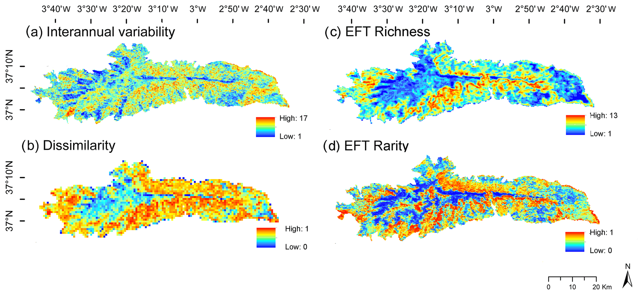
Figure 5Functional-diversity and functional-stability patterns based on the identification of EFTs derived from EVI images captured by the MOD13Q1-TERRA sensor along the 2001–2018 period. (a) EFT interannual variability for the period, i.e., the number of EFTs that occurred at each pixel throughout the period; (b) EFT interannual dissimilarity (1 – Jaccard index), i.e., the mean interannual dissimilarity of EFT composition in 4×4 MODIS-pixel windows between all possible combinations of pairs of years throughout the period; (c) spatial EFT richness patterns, i.e., the number of different EFTs observed in a 4×4 MODIS-pixel sliding window (232 m × 4=1 km2); (d) spatial EFT rarity patterns, i.e., a measure of the relative scarcity or abundance of each EFT in the study area.
5.2.3 Functional diversity at the ecosystem level
The highest EFT richness was observed in the Supramediterranean and Mesomediterranean belts (Fig. 5c). Such ecosystem functional-diversity hotspots (i.e., EFT hotspots) could be related to two facts. First, many Mediterranean mountains show high beta diversity (in terms of species turnover) around 1700–1900 m a.s.l. (Wilson and Shmida, 1984), where there is a great structural and compositional replacement of vegetation. Second, for the case of the Sierra Nevada, in the mid-mountain and especially on its southern face, there is a very diverse land cover mosaic composed of different types of natural vegetation (Valle et al., 2003), mixed with different types of pine afforestations, traditional croplands, and land uses (Camacho-Olmedo et al., 2002). The areas with the lowest EFT richness were located in the Oromediterranean and Cryoromediterranean belts and in the eastern semiarid Thermomediterranean extreme, where the harsh soil and climatic conditions (Peinado et al., 2019) diminish floristic diversity (Fernández Calzado et al., 2012). EFT rarity was highest in the peaks (above 2800 m a.s.l., Cryoromediterranean belt) and the lowest areas of the eastern side of the Sierra Nevada (semiarid Thermomediterranean belt), both areas characterized by a high concentration of narrowly endemic species (Mota et al., 2004; Cañadas et al., 2014; Peñas et al., 2019). The high-mountain areas (Oromediterranean belt) showed the lowest EFT rarity, since their EFT composition was the most abundant and extensive in the Biosphere Reserve. Mid-mountain areas (Supramediterranean and Mesomediterranean belts) (Fig. 5d) showed medium to high EFT-rarity values. The relatively higher rarity of ecosystem functioning in these belts was associated with the particular phenology of coniferous forests with fall–winter maxima, also identified in other areas of the Iberian Peninsula (Aragones et al., 2019).
5.2.4 Stability in the ecosystem functioning
The interannual variability ranged from 1 to 17 different EFTs over the 18-year period in the same pixel (Fig. 5a). The interannual variability and interannual dissimilarity (1 – Jaccard index) (Fig. 5b) observed were higher in the Supramediterranean and Mesomediterranean levels, coinciding with the altitudinal range where interannual climate variability is also higher (e.g., areas above the treeline are subjected to both cold–snowy years and warm–dry years, Zamora Rodríguez et al., 2016). The eastern end of the semiarid Thermomediterranean areas also displayed a high interannual variability. There also exists significant climate fluctuation in these areas, where small changes in the seasonal pattern of precipitation can produce large changes in primary production (Le Houérou et al., 1998; Cabello et al., 2012b). On the other hand, the most interannually stable areas (i.e., those that changed the least during the period) were located in the Meso-Oromediterranean and Cryoromediterranean belts, specifically, in the oak forests and high-mountain meadows, ecosystems that are subject to low human intervention.
We introduce a new dataset based on the processing and analysis of the temporal dynamics of the Enhanced Vegetation Index (EVI) data from the MODIS sensor (MOD13Q1.006). The dataset contains EFAs, EFTs, EFT richness and EFT rarity across the Sierra Nevada Biosphere Reserve (southeastern Spain). EFAs represent functional attributes at the ecosystem level related to primary production, seasonality, and phenology of carbon gains. EFTs are groups of pixels of the land surface that share similar dynamics in the exchanges of matter and energy between the biota and the physical environment, derived from the combination of the EFAs. EFT richness and EFT rarity are two metrics that provide information about the spatial heterogeneity of primary production as a focal ecosystem function. We also provide an estimation of the interannual stability of the former functional variables at both the pixel and landscape levels throughout the 2001–2018 period. For this, we estimated the EFT interannual variability at each pixel and the interannual dissimilarity in the composition of EFTs at a 4×4 sliding-window resolution. Overall, these data characterize the spatial and temporal patterns of a key measure of ecosystem functioning and ecosystem functional diversity. The EFT approach adopted here improves our understanding of ecosystem processes and ecosystem response through environmental gradients. It provides scientists and managers with valuable information to identify conservation priorities, assess ecosystem response to environmental changes, estimate ecosystem service provision, and model species distributions and ecological and hydrological processes.
The supplement related to this article is available online at: https://doi.org/10.5194/essd-15-1871-2023-supplement.
DAS, JC, JP, and BPC designed the study and DAS coordinated it. BPC and AR processed the images and produced the associated datasets presented in this paper. BPC prepared the manuscript with contributions from all the authors. BPC and JC wrote the definitive version of the manuscript. BPC, EG, and AJPL prepared the final figures. AJPL designed and made the application to visualize the data. AJPL and BPC prepared the Data Management Plan. All the authors reviewed the database and provided valuable feedback.
The contact author has declared that none of the authors has any competing interests.
Publisher's note: Copernicus Publications remains neutral with regard to jurisdictional claims in published maps and institutional affiliations.
Beatriz P. Cazorla was supported by the Plan Propio PhD program of the University of Almería. This research was developed as part of the projects EarthCul (reference PID2020-118041GB-I00), funded by the Spanish Ministry of Science and Innovation, Thematic Center on Mountain Ecosystem & Remote sensing, Deep learning-AI e-Services University of Granada-Sierra Nevada, Smart-EcoMountains, and INDALO (grant no. LifeWatch-2019-10-UGR-01) project, co-funded by the Ministry of Science and Innovation through the FEDER funds from the Spanish Pluriregional Operational Program 2014–2020 (POPE), LifeWatch-ERIC action line, within the Workpackages LifeWatch-2019-10-UGR-01_WP-8, LifeWatch-2019-10-UGR-01_WP-7, and LifeWatch-2019-10-UGR-01_WP-4;“ECOPOTENTIAL”: Improving future ecosystem benefits through earth observations (http://www.ecopotential-project.eu/, last access: 17 April 2023), which received funding from the European Union's Horizon 2020 research and innovation program under grant agreement no. 641762, project “Ecosystem and Socio-Ecosystem Functional Types: Integrating biophysical and social functions to characterize and map the ecosystems of the Anthropocene” (CGL2014-61610-EXP), which received funding from the Spanish Ministry of Economy and Business; Project LIFE-ADAPTAMED (LIFE14 CCA/ES/000612): “Protection of key ecosystem services by adaptive management of Climate Change endangered Mediterranean socio-ecosystems”. Emilio Guirado was supported by the Generalitat Valenciana and the European Social Fund (APOSTD/2021/188). This research was done under the collaboration of the LTSER platforms of the arid Iberian southeast, Spain, (LTER_EU_ES_027) and Sierra Nevada/Granada (ES-SNE), Spain (LTER_EU_ES_010) and contributes to the work done within the GEO BON working group on ecosystem function essential biodiversity variables.
This research has been supported by the Plan Propio PhD program of the University of Almería; projects EarthCul (reference PID2020-118041GB-I00); INDALO (grant no. LifeWatch-2019-10-UGR-01); LifeWatch-2019-10-UGR-01_WP-8, LifeWatch-2019-10-UGR-01_WP-7, and LifeWatch-2019-10-UGR-01_WP-4; ECOPOTENTIAL grant agreement no. 641762; “Ecosystem and Socio-Ecosystem Functional Types: Integrating biophysical and social functions to characterize and map the ecosystems of the Anthropocene” (CGL2014-61610-EXP); Project LIFE-ADAPTAMED (LIFE14 CCA/ES/000612); Generalitat Valenciana and the European Social Fund (APOSTD/2021/188).
This paper was edited by Kirsten Elger and reviewed by James Thornton and one anonymous referee.
Alcaraz-Segura, D., Paruelo, J., and Cabello, J.: Identification of current ecosystem functional types in the Iberian Peninsula, Global Ecol. Biogeogr., 15, 200–212, https://doi.org/10.1111/j.1466-822X.2006.00215.x, 2006.
Alcaraz-Segura, D., Cabello, J., Paruelo, J. M., and Delibes, M.: Use of Descriptors of Ecosystem Functioning for Monitoring a National Park Network: A Remote Sensing Approach, Environ. Manage., 43, 38–48, https://doi.org/10.1007/s00267-008-9154-y, 2009.
Alcaraz-Segura, D., Paruelo, J. M., Epstein, H. E., and Cabello, J.: Environmental and Human Controls of Ecosystem Functional Diversity in Temperate South America, Remote Sens, 5, 127–154, https://doi.org/10.3390/rs5010127, 2013.
Alcaraz-Segura, D., Lomba, A., Sousa-Silva, R., Nieto-Lugilde, D., Alves, P., Georges, D., Vicente, J. R., and Honrado, J. P.: Potential of satellite-derived Ecosystem Functional Attributes to anticipate species range shifts, Int. J. Appl Earth Obs. Geoinf., 57, 86–92, https://doi.org/10.1016/j.jag.2016.12.009, 2017.
Alcaraz-Segura, D., Blanco-Sacristán, J., Bagnato, C., Cintas, J., and Cazorla, B. P.: Ecosystem Functional Types (EFTs) code, Zenodo [code], https://doi.org/10.5281/zenodo.7524973, 2023.
Anderson, C. B.: Biodiversity monitoring, earth observations and the ecology of scale, Ecol. Lett., 21, 1572–1585, https://doi.org/10.1111/ele.13106, 2018.
Aragones, D., Rodriguez-Galiano, V. F., Caparros-Santiago, J. A., and Navarro-Cerrillo, R. M.: Could land surface phenology be used to discriminate Mediterranean pine species?, Int. J. Appl. Earth Obs. Geoinf., 78, 281–294, https://doi.org/10.1016/j.jag.2018.11.003, 2019.
Arenas-Castro, S., Gonçalves, J., Alves, P., Alcaraz-Segura, D., and Honrado, J. P.: Assessing the multiscale predictive ability of Ecosystem Functional Attributes for species distribution modelling, PLOS ONE, 13, e0199292, https://doi.org/10.1371/journal.pone.0199292, 2018.
Balvanera, P., Pfisterer, A. B., Buchmann, N., He, J.-S., Nakashizuka, T., Raffaelli, D., and Schmid, B.: Quantifying the evidence for biodiversity effects on ecosystem functioning and services, Ecol. Lett., 9, 1146–1156, https://doi.org/10.1111/j.1461-0248.2006.00963.x, 2006.
Blanca, G., Cueto, M., Martínez-Lirola, M. J., and Molero-Mesa, J.: Threatened vascular flora of Sierra Nevada (Southern Spain), Biol. Conserv., 85, 269–285, https://doi.org/10.1016/S0006-3207(97)00169-9, 1998.
Blanca, G., Cueto, M., and Romero, A. T.: Rareza y endemicidad en la flora vascular de Sierra Nevada, in Biología de la conservación de plantas en Sierra Nevada: Principios y retos para su preservación, Editorial Universidad de Granada, 325–343, ISBN 9788433865120, 2019.
Bennett, E. M., Cramer, W., Begossi, A., Cundill, G., Díaz, S., Egoh, B. N., Geijzendorffer, I. R., Krug, C. B., Lavorel, S., Lazos, E., Lebel, L., Martín-López, B., Meyfroidt, P., Mooney, H. A., Nel, J. L., Pascual, U., Prieur-Richard, A. H., Reyers, B., Roebeling, P., Seppelt, R., Solan, M., Tschakert, P., Tscharntke, T., Turner II, B. L., Veburg, P. H., Viglizzo, E. F., White, P. C. L., and Woodward, G.: Linking biodiversity, ecosystem services, and human well-being: three challenges for designing research for sustainability, Curr. Opin. Environ. Sustain., 14, 76–85, https://doi.org/10.1016/j.cosust.2015.03.007, 2015.
Box, E. O., Holben, B. N., and Kalb, V.: Accuracy of the AVHRR vegetation index as a predictor of biomass, primary productivity and net CO2 flux, Vegetatio, 80, 71–89, https://doi.org/10.1007/BF00048034, 1989.
Cabello, J., Fernández, N., Alcaraz-Segura, D., Oyonarte, C., Piñeiro, G., Altesor, A., Delibes, M., and Paruelo, J. M.: The ecosystem functioning dimension in conservation: insights from remote sensing, Biodivers. Conserv., 21, 3287–3305, https://doi.org/10.1007/s10531-012-0370-7, 2012a.
Cabello, J., Alcaraz-Segura, D., Ferrero, R., Castro, A. J., and Liras, E.: The role of vegetation and lithology in the spatial and inter-annual response of EVI to climate in drylands of Southeastern Spain, J. Arid Environ., 79, 76–83, 2012b.
Cabello, J., Lourenço, P., Reyes, A., and Alcaraz-Segura, D.: Ecosystem services assessment of national parks networks for functional diversity and carbon conservation strategies using remote sensing, in: Earth observation of ecosystem services, edited by: Alcaraz-Segura, D., Di Bella, C. M., and Straschnoy, J. V., CRC Press, Boca Raton,179–200, ISBN 13:978-1-4665-0589-6, 2013.
Cabello, J., Alcaraz-Segura, D., Reyes-Díez, A., Lourenço, P., Requena-Mullor, J., Bonache, J., Castillo, P., Valencia, S., Naya, J., Ramírez, L., and Serrada, J.: Sistema para el Seguimiento del funcionamiento de ecosistemas en la Red de Parques Nacionales de España mediante Teledetección, Revista de Teledetección, 46, 119–131, https://doi.org/10.4995/raet.2016.5731, 2016.
Calzado, M. R. F., Mesa, J. M., Merzouki, A., and Porcel, M. C.: Vascular plant diversity and climate change in the upper zone of Sierra Nevada, Spain, Plant Biosyst.-Plan Biosyst., 146, 1044–1053, https://doi.org/10.1080/11263504.2012.710273, 2012.
Camacho-Olmedo, M., García-Martínez, P., Jiménez-Olivencia, Y., Menor-Toribio, J., and PanizaCabrera, A.: Dinámica evolutiva del paisaje vegetal de la Alta Alpujarra granadina en la segunda mitad del s. XX, Cuad Geogr., 32, 25–42, 2002.
Cañadas, E. M., Fenu, G., Peñas, J., Lorite, J., Mattana, E., and Bacchetta, G.: Hotspots within hotspots: Endemic plant richness, environmental drivers, and implications for conservation, Biol. Conserv., 170, 282–291, https://doi.org/10.1016/j.biocon.2013.12.007, 2014.
Cazorla, B. P., Cabello, J., Peñas, J., Guirado, E.., Reyes-Díez, A., and Alcaraz-Segura, D.: Funcionamiento de la vegetación y diversidad funcional de los ecosistemas de Sierra Nevada, in Biología de la conservación de plantas en Sierra Nevada: Principios y retos para su preservación, Editorial Universidad de Granada, 325–343, ISBN 9788433865120, 2019.
Cazorla, B. P., Cabello, J., Reyes-Díez, A., Guirado, E., Peñas, J., Pérez-Luque, A J., and Alcaraz-Segura, D.: Ecosystem functioning and functional diversity of Sierra Nevada (SE Spain), University of Almería and Granada, PANGAEA [data set], https://doi.org/10.1594/PANGAEA.924792, 2020a.
Cazorla, B. P., Cabello, J., Penas, J., Garcillan, P. P., Reyes, A., and Alcaraz-Segura, D.: Incorporating Ecosystem Functional Diversity into Geographic Conservation Priorities Using Remotely Sensed Ecosystem Functional Types, Ecosystems, 24, 548–564, https://doi.org/10.1007/s10021-020-00533-4, 2020b.
Coops, N. C., Kearney, S. P., Bolton, D. K., and Radeloff, V. C.: Remotely-sensed productivity clusters capture global biodiversity patterns, Sci. Rep., 8, 16261, https://doi.org/10.1038/s41598-018-34162-8, 2018.
Costanza, R., Norton, B. G., and Haskell, B. D.: Ecosystem Health: New Goals for Environmental Management, Island Press, ISBN 1-555963-141-4, 1992.
Didan, K., Munoz, A. B., Solano, R., and Huete, A.: MODIS vegetation index user's guide (MOD13 series), Vegetation Index and Phenology Lab, University of Arizona, https://modis-land.gsfc.nasa.gov/pdf/MOD13_User_Guide_V61.pdf (last access: 17 April 2023), 2015.
Duro, D. C., Coops, N. C., Wulder, M. A., and Han, T.: Development of a large area biodiversity monitoring system driven by remote sensing, Prog. Phys. Geogr., 31, 235–260, https://doi.org/10.1177/0309133307079054, 2007.
Fernández, N., Paruelo, J. M., and Delibes, M.: Ecosystem functioning of protected and altered Mediterranean environments: A remote sensing classification in Doñana, Spain, Remote Sens. Environ., 114, 211–220, https://doi.org/10.1016/j.rse.2009.09.001, 2010.
Fernández Calzado, M. R., Molero Mesa, J., Merzouki, A., and Casares Porcel, M.: Vascular plant diversity and climate change in the upper zone of Sierra Nevada, Spain, Plant Biosyst.-Plan Biosyst., 146, 1044–1053, https://doi.org/10.1080/11263504.2012.710273, 2012.
Geerken, R. A.: An algorithm to classify and monitor seasonal variations in vegetation phenologies and their inter-annual change, ISPRS J. Photogram. Remots. Sens., 64, 422–431, https://doi.org/10.1016/j.isprsjprs.2009.03.001, 2009.
Gorelick, N., Hancher, M., Dixon, M., Ilyushchenko, S., Thau, D., and Moore, R.: Google Earth Engine: Planetary-scale geospatial analysis for everyone, Remote Sens. Environ., 202, 18–27, https://doi.org/10.1016/j.rse.2017.06.031, 2017.
Grêt-Regamey, A., Brunner, S. H., and Kienast, F.: Mountain ecosystem services: who cares?, Mt. Res. Dev., 32, 32–45, https://doi.org/10.1659/MRD-JOURNAL-D-10-00115.S1, 2012.
Haines-Young, R. and Potschin, M.: The links between biodiversity, ecosystem services and human well-being, Ecosyst. Ecol., 1, 110–139, https://doi.org/10.1017/CBO9780511750458.007, 2010.
Huete, A., Justice, C., and Van Leeuwen, W.: MODIS vegetation index (MOD13), Algorithm theoretical basis document, NASA EOS-MODIS, 3 pp., https://modis.gsfc.nasa.gov/data/atbd/atbd_mod13.pdf (last access: 17 April 2023), 1999.
Huete, A., Didan, K., Miura, T., Rodriguez, E. P., Gao, X., and Ferreira, L. G.: Overview of the radiometric and biophysical performance of the MODIS vegetation indices, Remote Sens. Environ., 83, 195–213, https://doi.org/10.1016/S0034-4257(02)00096-2, 2002.
Huete, A. R., Liu, H. Q., Batchily, K. V., and Van Leeuwen, W. J. D. A.: A comparison of vegetation indices over a global set of TM images for EOS-MODIS, Remote Sens. Environ., 59, 440–451, https://doi.org/10.1016/S0034-4257(96)00112-5, 1997.
Ivits, E., Cherlet, M., Mehl, W., and Sommer, S.: Ecosystem functional units characterized by satellite observed phenology and productivity gradients: A case study for Europe, Ecol Indic., 27, 17–28, https://doi.org/10.1016/j.ecolind.2012.11.010, 2013.
Jaccard, P.: Étude comparative de la distribution florale dans une portion des Alpes et des Jura, Bull. Soc. Vaudoise Sci. Nat., 37, 547–579, 1901.
Jax, K.: Ecosystem Functioning, Cambridge University Press, Cambridge, ISBN 978-0-521-70523-3, 2010.
Karlsen, S. R., Elvebakk, A., Høgda, K. A., and Johansen, B.: Satellite-based mapping of the growing season and bioclimatic zones in Fennoscandia, Global Ecol. Biogeogr., 15, 416–430, https://doi.org/10.1111/j.1466-822X.2006.00234.x, 2006.
Lee, S.-J., Berbery, E. H., and Alcaraz-Segura, D.: The impact of ecosystem functional type changes on the La Plata Basin climate, Adv. Atmos. Sci., 30, 1387–1405, https://doi.org/10.1007/s00376-012-2149-x, 2013.
Le Houérou, H. N.: A probabilistic approach to assessing arid rangelands' productivity, carrying capacity and stocking rates, in: Drylands: Sustainable Use of Rangelands into the Twenty First Century, edited by: Squires, V. R. and Sidahmed, A. E., IFAD, Rome, Italy, 1998.
Lorite, J.: An updated checklist of the vascular flora of Sierra Nevada (SE Spain), Phytotaxa, 261, 1–57, 2016.
Lorite, J., Ros-Candeira, A., Alcaraz-Segura, D., Salazar-Mendías, C.: FloraSNevada: a trait database of the vascular flora of Sierra Nevada, southeast Spain, Ecology, 101, e03091, https://doi.org/10.1002/ecy.3091, 2020.
Mace, G. M., Reyers, B., Alkemade, R., Biggs, R., Chapin, F. S., Cornell, S. E., Díaz, S., Jennings, S., Leadley, P., Mumby, P. J., Purvis, A., Scholes, R. J., Seddon, A. W. R., Solan, M., Steffen, W., and Woodward, G.: Approaches to defining a planetary boundary for biodiversity, Global Environ. Change, 28, 289–297, https://doi.org/10.1016/j.gloenvcha.2014.07.009, 2014.
Molero, J. and Marfil, J. M.: The bioclimates of Sierra Nevada National Park, Int. J. Geobot. Res., 5, 1–11, https://doi.org/10.1007/978-3-319-54867-8_4, 2015.
Mota, J. F., Sola, A. J., Jiménez-Sánchez, M. L., Pérez-García, F., and Merlo, M. E.: Gypsicolous flora, conservation and restoration of quarries in the southeast of the Iberian Peninsula, Biodivers. Conserv., 13, 1797–1808, https://doi.org/10.1023/B:BIOC.0000035866.59091.e5, 2004.
Mouchet, M. A., Villéger, S., Mason, N. W. H., and Mouillot, D.: Functional diversity measures: an overview of their redundancy and their ability to discriminate community assembly rules, Funct. Ecol., 24, 867–876, https://doi.org/10.1111/j.1365-2435.2010.01695.x, 2010.
Mucina, L.: Biome: evolution of a crucial ecological and biogeographical concept, New Phytol., 222, 97–114, https://doi.org/10.1111/nph.15609, 2019.
Müller, O. V., Berbery, E. H., Alcaraz-Segura, D., and Ek, M. B.: Regional Model Simulations of the 2008 Drought in Southern South America Using a Consistent Set of Land Surface Properties, J. Climate, 590, 6754–6778, https://doi.org/10.1175/JCLI-D-13-00463.1, 2014.
Oki, T., Blyth, E. M., Berbery, E. H., and Alcaraz-Segura, D.: Land Use and Land Cover Changes and Their Impacts on Hydroclimate, Ecosystems and Society, in: Climate Science for Serving Society: Research, Modeling and Prediction Priorities, edited by: Asrar, G. R. and Hurrell, J. W., Springer Netherlands, Dordrecht, 185–203, https://doi.org/10.1007/978-94-007-6692-1_7, 2013.
Paruelo, J. M. and Lauenroth, W. K.: Regional patterns of normalized difference vegetation index in North American shrublands and grasslands, Ecology, 76, 1888–1898, https://doi.org/10.2307/1940721, 1995.
Paruelo, J. M., Jobbágy, E. G., and Sala, O. E.: Current Distribution of Ecosystem Functional Types in Temperate South America, Ecosystems, 4, 683–698, https://doi.org/10.1007/s10021-001-0037-9, 2001.
Peinado, F. J. M., Morales, M. N. J., and Ondoño, E. F.: Los suelos de Sierra Nevada, su relación con la litología y la vegetación, in Biología de la conservación de plantas en Sierra Nevada: Principios y retos para su preservación, Editorial Universidad de Granada, 173–192, ISBN 9788433865120, 2019.
Pelkey, N. W., Stoner, C. J., and Caro, T. M.: Assessing habitat protection regimes in Tanzania using AVHRR NDVI composites: Comparisons at different spatial and temporal scales, Int. J. Remote Sens., 24, 2533–2558, https://doi.org/10.1080/01431160210155929, 2003.
Peñas, J., Sánchez, E. C., and del Río Sánchez, J.: Fitogeografía de Sierra Nevada e implicaciones para la conservación, in Biología de la conservación de plantas en Sierra Nevada: Principios y retos para su preservación, Editorial Universidad de Granada, 81–116, ISBN 9788433865137, 2019.
Pereira, H. M., Ferrier, S., Walters, M., Geller, G. N., Jongman, R. H. G., Scholes, R. J., Bruford, M. W., Brummitt, N., Butchart, S. H. M., Cardoso, A. C., Coops, N. C., Dulloo, E., Faith, D. P., Freyhof, J., Gregory, 540 R. D., Heip, C., Höft, R., Hurtt, G., Jetz, W., Karp, D. S., McGeoch, M. A., Obura, D., Onoda, Y., Pettorelli, N., Reyers, B., Sayre, R., Scharlemann, J. P. W., Stuart, S. N., Turak, E., Walpole, M., and Wegmann, M.: Essential Biodiversity Variables, Science, 339, 277–278, https://doi.org/10.1126/science.1229931, 2013.
Pérez-Hoyos, A., Martínez, B., García-Haro, F. J., Moreno, Á., and Gilabert, M. A.: Identification of Ecosystem Functional Types from Coarse Resolution Imagery Using a Self-Organizing Map Approach: A Case Study for Spain, Remote Sens., 6, 11391–11419, https://doi.org/10.3390/rs61111391, 2014.
Pérez-Luque, A. J., Bonet, F. J., Pérez-Pérez, R., Aspizua, R., Lorite, J., and Zamora, R.: Sinfonevada: Dataset of floristic diversity in Sierra Nevada forests (SE Spain), PhytoKeys, 35, 1–15, https://doi.org/10.3897/phytokeys.35.6363, 2014.
Pérez-Luque, A. J., Pérez-Pérez, R., Bonet-García, F. J., and Magaña, P. J.: An ontological system based on MODIS images to assess ecosystem functioning of Natura 2000 habitats: A case study for Quercus pyrenaica forests, Int. J. Appl. Earth Obs. Geoinf., 37, 142–151, https://doi.org/10.1016/j.jag.2014.09.003, 2015a.
Pérez-Luque, A. J., Zamora, R., Bonet, F. J., and Pérez-Pérez, R.: Dataset of MIGRAME Project (Global Change, Altitudinal Range Shift and Colonization of Degraded Habitats in Mediterranean Mountains), PhytoKeys, 56, 61–81, https://doi.org/10.3897/phytokeys.56.5482, 2015b.
Pérez-Luque, A. J., Sánchez-Rojas, C. P., Zamora, R., Pérez-Pérez, R., and Bonet, F. J.: Dataset of Phenology of Mediterranean high-mountain meadows flora (Sierra Nevada, Spain), PhytoKeys, 46, 89–107, https://doi.org/10.3897/phytokeys.46.9116, 2015c.
Pérez-Luque, A. J., Barea-Azcón, J. M., Álvarez-Ruiz, L., Bonet-García, F. J., and Zamora, R.: Dataset of Passerine bird communities in a Mediterranean high mountain (Sierra Nevada, Spain), ZooKeys, 552, 137–154, https://doi.org/10.3897/zookeys.552.6934, 2016.
Pérez-Luque, A. J., Bonet-García, F. J., and Zamora Rodríguez, R.: Map of ecosystems types in Sierra Nevada mountain (southern Spain), PANGAEA [data set], https://doi.org/10.1594/PANGAEA.910176, 2019.
Pérez-Luque, A. J., Cazorla, B. P., Cabello, J., Reyes, A., Guirado, E., Peñas, J., and Alcaraz-Segura, D.: Ecosystem functioning and functional diversity of Sierra Nevada, [data set], http://obsnev.es/apps/efts_SN.html, last access: 17 April 2023.
Petchey, O. L. and Gaston, K. J.: Functional diversity: back to basics and looking forward, Ecol. Lett., 9, 741–758, https://doi.org/10.1111/j.1461-0248.2006.00924.x, 2006.
Pettorelli, N., Vik, J. O., Mysterud, A., Gaillard, J.-M., Tucker, C. J., and Stenseth, N. Chr.: Using the satellite-derived NDVI to assess ecological responses to environmental change, Trends Ecol. Evol., 20, 503–510, https://doi.org/10.1016/j.tree.2005.05.011, 2005.
Pettorelli, N., Wegmann, M., Skidmore, A., Mücher, S., Dawson, T. P., Fernandez, M., Lucas, R., Schaepman, M. E., Wang, T., O'Connor, B., Jongman, R. H. G., Kempeneers, P., Sonnenschein, R., Leidner, A. K., Böhm, M., He, K. S., Nagendra, H., Dubois, G., Fatoyinbo, T., Hansen, M. C., Paganini, M., de Klerk, H. M., Asner, G. P., Kerr, J. T., Estes, A. B., Schmeller, D. S., Heiden, U., Rocchini, D., Pereira, H. M., Turak, E., Fernandez, N., Lausch, A., Cho, M. A., Alcaraz-Segura, D., McGeoch, M. A., Turner, W., Mueller, A., St-Louis, V., Penner, J., Vihervaara, P., Belward, A., Reyers, B., and Geller, G. N.: Framing the concept of satellite remote sensing essential biodiversity variables: challenges and future directions, Remote Sens. Ecol. Conserv., 2, 122–131, https://doi.org/10.1002/rse2.15, 2016.
Pettorelli, N., Schulte to Bühne, H., Tulloch, A., Dubois, G., Macinnis-Ng, C., Queirós, A. M., Keith, D. A., Wegmann, M., Schrodt, F., Stellmes, M., Sonnenschein, R., Geller, G. N., Roy, S., Somers, B., Murray, N., Bland, L., Geijzendorffer, I., Kerr, J. T., Broszeit, S., Leitão, P. J., Duncan, C., Serafy, G. E., He, K. S., Blanchard, J. L., Lucas, R., Mairota, P., Webb, T. J., and Nicholson, E.: Satellite remote sensing of ecosystem functions: opportunities, challenges and way forward, Remote Sens. Ecol. Conserv., 4, 71–93, https://doi.org/10.1002/rse2.59, 2018.
Regos, A., Gagne, L., Alcaraz-Segura, D., Honrado, J. P., and Domínguez, J.: Effects of species traits and environmental predictors on performance and transferability of ecological niche models, Sci. Rep., 9, 1–14, https://doi.org/10.1038/s41598-019-40766-5, 2019.
Requena-Mullor, J. M., López, E., Castro, A. J., Alcaraz-Segura, D., Castro, H., Reyes, A., and Cabello, J.: Remote-sensing based approach to forecast habitat quality under climate change scenarios, PLOS ONE, 12, e0172107, https://doi.org/10.1371/journal.pone.0172107, 2017.
Ros-Candeira, A., Pérez-Luque, A. J., Suárez-Muñoz, M., Bonet-García, F. J., Hódar, J. A., Giménez de Azcárate, F., and Ortega-Díaz, E.: Dataset of occurrence and incidence of pine processionary moth in Andalusia, south Spain, ZooKeys, 852, 125–136, https://doi.org/10.3897/zookeys.852.28567, 2019.
Ros-Candeira, A., Moreno-Llorca, R., Alcaraz-Segura, D., Bonet-García, F. J., and Vaz, A. S.: Social media photo content for Sierra Nevada: a dataset to support the assessment of cultural ecosystem services in protected areas, Nat. Conserv., 38, 1–12, 2020.
Running, S. W., Thornton, P. E., Nemani, R., and Glassy, J. M.: Global Terrestrial Gross and Net Primary Productivity from the Earth Observing System, in: Methods in Ecosystem Science, edited by: Sala, O. E., Jackson, R. B., Mooney, H. A., and Howarth, R. W., Springer New York, New York, NY, 44–57, https://doi.org/10.1007/978-1-4612-1224-9_4, 2000.
Skidmore, A. K., Pettorelli, N., Coops, N. C., Geller, G. N., Hansen, M., Lucas, R., Mücher, C. A., O'Connor, B., Paganini, M., Pereira, H. M., Schaepman, M. E., Turner, W., Wang, T., and Wegmann, M.: Environmental science: Agree on biodiversity metrics to track from space, Nature, 523, 403–405, https://doi.org/10.1038/523403a, 2015.
Skidmore, A. K., Coops, N. C., Neinavaz, E., Ali, A., Schaepman, M. E., Paganini, M., Kissling, W. D., Vihervaara, P., Darvishzadeh, R., Feihauer, H., Fernandez, M., Fernandez, N., Gorelick, N., Geijzendorffer, I., Heiden, U., Heurich, M., Hobern, D., Holzwarth, S., Muller-Karger, F. E., Van De Kervoche, R., Lausch, A., Leitao, P. J., Lock, M. C., Mücher, C. A., O'Connor, B., Rocchini, D., Roeoesli, C., Turner, W., Vis, J. K., Wang, T., Wegmann, M., and Wingate, V.: Priority list of biodiversity metrics to observe from space, Nat. Ecol. Evol., 5, 896–906, https://doi.org/10.1038/s41559-021-01451-x, 2021.
Steffen, W., Richardson, K., Rockström, J., Cornell, S. E., Fetzer, I., Bennett, E. M., Biggs, R., Carpenter, S. R., de Vries, W., de Wit, C. A., Folke, C., Gerten, D., Heinke, J., Mace, G. M., Persson, L. M., Ramanathan, V., Reyers, B., and Sörlin, S.: Planetary boundaries: Guiding human development on a changing planet, Science, 347, 1259855, https://doi.org/10.1126/science.1259855, 2015.
Townshend, J. R., Goff, T. E., and Tucker, C. J.: Multitemporal dimensionality of images of normalized difference vegetation index at continental scales, IEEE T. Geosci. Remote, 6, 888–895, https://doi.org/10.1109/TGRS.1985.289474, 1985.
Valle, F., Algarra, J. A., Arrojo, E., Asensi, A., Cabello, J., Cano, E., Cañadas Sánchez, E., Cueto, M., Dana, E., and Simón, D.: Mapa de series de vegetación de Andalucía, ISBN 84-7207-137-5, 2003.
Villarreal, S., Guevara, M., Alcaraz-Segura, D., Brunsell, N. A., Hayes, D., Loescher, H. W., and Vargas, R.: Ecosystem functional diversity and the representativeness of environmental networks across the conterminous United States, Agr. Forest Meteorol., 262, 423–433, https://doi.org/10.1016/j.agrformet.2018.07.016, 2018.
Virginia, R. A., Wall, D. H., and Levin, S. A.: Principles of ecosystem function, Encycloped. Biodivers., 2, 345–352, 2001.
Wang, Y. and Huang, F.: Identification and analysis of ecosystem functional types in the west of Songnen Plain, China, based on moderate resolution imaging spectroradiometer data, J. Appl. Remote Sens., 9, 096096, https://doi.org/10.1117/1.JRS.9.096096, 2015.
Wilson, M. V. and Shmida, A.: Measuring beta diversity with presence-absence data, J. Ecol., 72, 1055–1064, https://doi.org/10.2307/2259551, 1984.
Xiao, J., Chevallier, F., Gomez, C., Guanter, L., Hicke, J. A., Huete, A. R., Ichii, K., Ni, W., Pang, Y., Rahman, A. F., Sun, G., Yuan, W., Zhang, L., and Zhang, X.: Remote sensing of the terrestrial carbon cycle: A review of advances over 50 years, Remote Sens. Environ., 233, 111383, https://doi.org/10.1016/j.rse.2019.111383, 2019.
Zamora, R., Pérez-Luque, A. J., Bonet, F. J., Barea-Azcón, J. M., Aspizua, R., Sánchez-Gutiérrez, F. J., Cano-Manuel, F. J., Ramos-Losada, B., and Henares-Civantos, I.: Global Change Impact in the Sierra Nevada Long-Term Ecological Research Site (Southern Spain), Bull. Ecol. Soc. Am., 98, 157–164, https://doi.org/10.1002/bes2.1308, 2017.
Zamora Rodríguez, R. J., Pérez-Luque, A. J., Bonet, F. J., Barea-Azcón, J. M., and Aspizua, R.: Global Change Impacts in Sierra Nevada: Challenges for Conservation, Consejería de Medio Ambiente y Ordenación del Terriorio, Junta de Andalucía, 208 pp., ISBN 978-84-338-5960-0, 2016.