Global Ozone Monitoring Experiment-2 (GOME-2) daily and monthly level-3 products of atmospheric trace gas columns

We introduce the new Global Ozone Monitoring Experiment-2 (GOME-2) daily and monthly level-3 product of total column ozone (O₃), total and tropospheric column nitrogen dioxide (NO₂), total column water vapour, total column bromine oxide (BrO), total column formaldehyde (HCHO), and total column sulfur dioxide (SO₂) (daily products https://doi.org/10.15770/EUM_SAF_AC_0048, AC SAF, 2023a; monthly products https://doi.org/10.15770/EUM_SAF_AC_0049, AC SAF, 2023b). The GOME-2 level-3 products aim to provide easily translatable and user-friendly data sets to the scientific community for scientific progress as well as to satisfy public interest. The purpose of this paper is to present the theoretical basis as well as the verification and validation of the GOME-2 daily and monthly level-3 products.

The GOME-2 level-3 products are produced using the overlapping area-weighting method. Details of the gridding algorithm are presented. The spatial resolution of the GOME-2 level-3 products is selected based on the sensitivity study. The consistency of the resulting level-3 products among three GOME-2 sensors is investigated through time series of global averages, zonal averages, and bias. The accuracy of the products is validated by comparison to ground-based observations. The verification and validation results show that the GOME-2 level-3 products are consistent with the level-2 data. Small discrepancies are found among three GOME-2 sensors, which are mainly caused by the differences in the instrument characteristic and level-2 processor. The comparison of GOME-2 level-3 products to ground-based observations in general shows very good agreement, indicating that the products are consistent and fulfil the requirements to serve the scientific community and general public.

1 Introduction

Satellite remote-sensing observations provide indispensable spatiotemporal information on atmospheric composition at a global scale. Various atmospheric trace gases can be retrieved from nadir-viewing satellite spectroscopic observations in the ultraviolet (UV) and visible (VIS) spectral ranges. This type of observation has long been conducted since the Global Ozone Monitoring Experiment (GOME) mission launched in 1995 (Burrows et al., 1999). Together with other follow-up satellite-borne spectrometers, for example the SCanning Imaging Absorption SpectroMeter for Atmospheric CHartographY (SCIAMACHY; Bovensmann et al., 1999), Global Ozone Monitoring Experiment-2 (GOME-2; Callies et al., 2000), Ozone Monitoring Instrument (OMI; Levelt et al., 2006), and TROPOspheric Monitoring Instrument (TROPOMI; Veefkind et al., 2012), these observations provide a global record of earthshine radiance in the UV, VIS, and near-infrared (NIR) (UVN) spectral ranges for more than 25 years. The processing of satellite observation of the trace gas column involves two major steps, (1) conversion of raw spectral channel counts (level-0 data) to geolocation and radiometric calibrated radiance and irradiance data (level-1B data) and (2) the retrieval of trace gas columns (level-2 data) from level-1B data, which include spectral retrieval of trace gas slant columns and subsequently convert them to vertical columns. To ensure the accuracy and consistency of satellite observations, GOME-2 data are processed in stable operational environments within the framework of Satellite Application Facility on Atmospheric Composition Monitoring (AC SAF). The level-0 to level-1B conversion is processed by the European Organisation for the Exploitation of Meteorological Satellites (EUMETSAT), while the level-1B to level-2 conversion is processed by the German Aerospace Center (DLR).

The GOME-2 level-2 data are orbital-swath scientific products. A level-2 data file contains observations within a single orbit. Trace gas columns are expressed in the satellite-viewing geometry of reference using across-track and along-track positions. In addition, the satellite measurement footprint is not in a regular latitude–longitude grid, and often multiple pixels overlap at the edges of an orbit within a day. Using this kind of scientific product requires very good knowledge of the satellite product, especially when averaging multiple measurements to generate daily or monthly maps. In order to provide a user-friendly satellite product, we have projected the GOME-2 level-2 data onto a regular latitude–longitude grid to generate operational level-3 products. The purpose of this document is to present the theoretical basis, verification, and validation of the GOME-2 level-3 daily and monthly gridded products. These products include global daily and monthly means of total column ozone (O₃), total and tropospheric column nitrogen dioxide (NO₂), total column bromine oxide (BrO), total column water vapour (H₂O), total column formaldehyde (HCHO), and total column sulfur dioxide (SO₂). Compared to satellite observations from OMI and TROPOMI, which measure at noon or in the early afternoon, GOME-2 measurements in the morning provide addition information on the temporal/diurnal variation of these atmospheric trace gases.

The paper is organized as follows. Section 2.1 describes the GOME-2 instruments. A brief description of each GOME-2 level-2 trace gas product can be found in Sect. 2.2, while auxiliary data sets used for comparison are presented in Sect. 2.3. The gridding algorithm for level-2 to level-3 processing is presented in Sect. 3.1. Section 3.2 shows the selection of the best spatial resolution for GOME-2 level-3 data. The verification and validation methodology are presented in Sect. 3.3. Section 4 presents the resulting daily and monthly level-3 products. Results for the verification and validation of GOME-2 level-3 data are presented in Sect. 5. Finally, Sect. 7 summarizes our findings.

2 Instruments and data sets

The GOME-2 instruments and the operational level-2 products of each trace gas used for the generation of gridded level-3 data are described in this section. Ground-based measurements used to validate the GOME-2 level-3 products are also presented.

2.1 GOME-2 instruments

GOME-2 instruments are passive nadir-viewing satellite-borne spectrometers on board the European Organization for the EUMETSAT Metop series of satellites. The Metop satellites orbit at an altitude of ∼ 820 km on sun-synchronous orbits with a 29 d (412-orbit) repeat cycle and a local Equator overpass time of 09:30 LT (local time) on the descending node. Metop-A, the first Metop satellite, was launched on 19 October 2006. Metop-B was launched 6 years later on 17 September 2012. The third Metop satellite, Metop-C, was launched on 7 November 2018. A more detailed introduction of the Metop series of satellites can be found in Klaes et al. (2007).

The GOME-2 instruments are optical spectrometers equipped with scanning mirrors which enable across-track scanning in nadir and sideways viewing for polar coverage (Callies et al., 2000). Each GOME-2 instrument consists of four detectors covering a wavelength range of 240–790 nm with a spectral resolution ranging from 0.26 to 0.51 nm. Additionally, two polarization components are measured with polarization measurement devices (PMDs) using 30 broadband channels covering the full spectral range at higher spatial resolution. The nominal spatial resolution of the instruments is 80 km (across-track) × 40 km (along-track) for the forward scan, and the spatial resolution is reduced to 240 km (across-track) × 40 km (along-track) for the backward scan. The scanning swath width of the GOME-2 instruments is about 1920 km. After the GOME-2 instrument on board the Metop-B satellite (referred to as GOME-2B hereafter) went into tandem operation with Metop-A in July 2013, the across-track spatial resolution of the GOME-2 instrument on board the Metop-A satellite (referred to as GOME-2A hereafter) was doubled to 40 km, with the spatial coverage of a swath reduced to 960 km. The spatial resolution and coverage of GOME-2B remain unchanged. A more detailed description of the GOME-2 instruments can be found in Munro et al. (2016). Table 1 summarizes the major characteristics of all three GOME-2 instruments.

Table 1 Summary of the GOME-2 instrument characteristics.

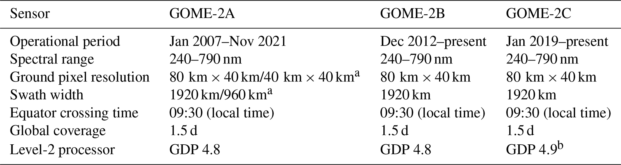
^a Since tandem operation with GOME-2B on 15 July 2013. ^b GDP 4.9 was introduced for GOME-2C and includes updated instrument-specific retrieval settings for NO₂ and SO₂. For NO₂, the alternative DOAS fitting window 430.2–465 nm is used (because of calibration issues for GOME-2C for wavelengths <430 nm). For SO₂, improved DOAS fitting settings are used, and the wavelength region has been changed to 312–325 nm (Valks et al., 2019).

2.2 Operational GOME-2 level-2 data

2.2.1 Total column ozone

Ozone (O₃) is an important trace gas in the earth’s atmosphere. In the stratosphere, ozone absorbs ultraviolet radiation from the sun, thus protecting the biosphere from harmful radiation (Eleftheratos et al., 2013; Hegglin et al., 2015). In the lower troposphere, natural ozone has an equally important beneficial role, because it initiates the chemical removal of air pollutants and greenhouse gases from the atmosphere, such as carbon monoxide (CO), nitrogen oxides (NO_x), and methane (CH₄). However, ozone at high concentration can also be harmful to humans, plants, and animals. In addition, ozone is a greenhouse gas that contributes to the warming of the earth’s atmosphere. In both the stratosphere and the troposphere, ozone absorbs infrared radiation emitted from the earth’s surface, trapping heat in the atmosphere. As a result, increases or decreases in stratospheric or tropospheric ozone induce a climate forcing (Hegglin et al., 2015).

The retrieval of total column ozone from GOME-2 (ir)radiance spectra is based on the typical two-step approach for weakly absorbing trace gas. The first step is to apply the differential optical absorption spectroscopy (DOAS) technique (Platt and Stutz, 2008) to the GOME-2 (ir)radiance spectra within the wavelength range of 325–335 nm to retrieve ozone slant column densities (SCDs). Ozone absorption features are prominent in this wavelength range. In addition, GOME-2 measurements have high signal-to-noise and manageable interference effects from other trace gases in this wavelength band. The DOAS fits include two ozone cross sections at 218 and 243 K. A NO₂ cross section and the Ring spectrum are also included in the spectral fit.

The second step is the conversion of retrieved ozone slant column densities to vertical column densities (VCDs) using air mass factors (AMFs) (Solomon et al., 1987; Palmer et al., 2001). Vertical distribution profiles are essential a priori information used in the calculation of AMFs. The air mass factor calculation for ozone vertical column retrieval follows an iterative approach. The algorithm uses a standard ozone profile to retrieve an initial ozone vertical column. Based on the initial result of the ozone vertical column retrieval, the algorithm selects the most appropriate a priori profile from the climatology database and uses it a priori in the next iteration. The iterations end when the change in the retrieved vertical column is less than 0.1 % or when it reaches the maximum limit of iterations. For GOME-2 total column ozone retrieval, the number of iterations is in most cases smaller than 4. The radiative transfer model, LInearized Discrate Ordinate Radiative Transfer (LIDORT) (Spurr, 2008), is used for the radiative transfer calculation of AMFs with respect to the a priori ozone profile and cloud information. Cloud parameters are retrieved from GOME-2 measurements using the optical cloud recognition algorithm (OCRA) and retrieval of cloud information using neural network (ROCINN) algorithms (see Sect. 2.2.7), and the ozone absorption inside and below the cloud is treated by the intra-cloud correction term, which is a function of solar zenith angle and cloud albedo. AMFs are computed at a single wavelength of 325.5 nm (Van Roozendael et al., 2006). As the major part of ozone is in the stratosphere, which is well above clouds, all measurements (cloudy and clear-sky) are used in the level-3 product. More details on the GOME-2 total column ozone retrieval can be found in Loyola et al. (2011) and Hao et al. (2014).

2.2.2 Total and tropospheric column nitrogen dioxide

Nitrogen dioxide (NO₂) plays an important role in atmospheric chemistry and air quality in the troposphere. It is an air pollutant affecting human health and ecosystems. Furthermore, NO₂ in the troposphere is a major ozone precursor while being a catalyst of stratospheric ozone depletion processes, which is very important for climate change studies due to its indirect effect on the global climate (Shindell et al., 2009).

The retrieval of total and tropospheric column NO₂ from GOME-2 follows the typical two-step approach for a weakly absorbing trace gas. The DOAS approach is applied to GOME-2 (ir)radiance spectra to determine NO₂ slant column densities at a wavelength range of 425–450 nm (Valks et al., 2011) for GOME-2/Metop-A and GOME-2/Metop-B (GDP – GOME Data Processor – 4.8). NO₂ absorption structures are prominent, and the interference effects are manageable within this spectral window. In addition, GOME-2 measurements have a high signal-to-noise ratio in this wavelength band. For GOME-2/Metop-C (GDP 4.9), an alternative fitting window of 430.2–465 nm is used, as there are systematic structures in the DOAS fitting residual for GOME-2C for wavelengths <430 nm, which result in a large positive bias of ∼ 30 %. A single NO₂ reference cross-sectional spectrum at 240 K (Vandaele et al., 2002), the interfering species ozone, O₄ and H₂O, and the Ring spectrum are included in the DOAS spectral retrieval. The temperature dependence of the NO₂ absorption cross section has been taken into account in the air mass factor calculation to improve the accuracy of the retrieved columns.

The initial total VCD is retrieved assuming an unpolluted troposphere. Therefore, the air mass factor is weighted toward stratospheric NO₂, whereas the tropospheric NO₂ amount is assumed to be negligible. This assumption is valid over large parts of the earth, but in areas with significant tropospheric NO₂, the total column densities are underestimated and need to be corrected. The air mass factors are calculated at the mid-point of the spectral-fitting window at 437.5 nm using the radiative transfer model LIDORT. A harmonic climatology of stratospheric NO₂ profiles is used in the air mass factor calculation to incorporate the seasonal and latitudinal variation of stratospheric NO₂. Stratospheric NO₂ columns are estimated using the spatial filtering approach (Wenig et al., 2004; Valks et al., 2011). This method masks out potentially polluted areas and then applies a low-pass filter in the zonal direction to derive the stratospheric component. The tropospheric NO₂ vertical columns are then derived from the residual tropospheric slant columns using a more accurate tropospheric air mass factor which considers the effects of clouds and the NO₂ profile from a chemistry transport model. The derived tropospheric columns are used to correct the initial total NO₂ columns under polluted conditions to provide an estimate of total vertical columns.

Monthly average NO₂ profiles during the GOME-2 overpass time from the chemistry transport model MOZART-2 are used in the tropospheric air mass factor calculations. Cloud properties derived from GOME-2 using the OCRA and ROCINN algorithms (see Sect. 2.2.7) are used in the calculation of air mass factors in the case of (partly) cloudy conditions. The Clouds-As-Layers (CAL) model included in OCRA/ROCINN has also been implemented in our prototype GOME-2 NO₂ algorithm, as described in Liu et al. (2020). The new NO₂ algorithm uses an improved directionally dependent Lambertian-equivalent reflectivity (DLER) for AMF calculation. It is planned to implement the prototype GOME-2 NO₂ algorithm in a future version of the operational GDP. The calculation of AMFs for (partly) cloudy conditions uses the independent pixel approximation. For measurements over cloudy scenes, the cloud top is usually well above the NO₂ pollution in the boundary layer. When the clouds are optically thick, the enhanced tropospheric NO₂ concentrations cannot be detected by the satellite, which can result in large errors. Therefore, GOME-2 measurements with a cloud radiance fraction >50 % are flagged in the level-2 data and filtered in the computation of the level-3 tropospheric NO₂ product. More details of the GOME-2 total and tropospheric column NO₂ retrieval can be found in Valks et al. (2011).

2.2.3 Total column water vapour

Water vapour is one of the major components in the atmosphere, with strong impacts on climate and weather, due to its abundance in the atmosphere, making it the most important natural greenhouse gas, accounting for more than 60 % of the greenhouse effect (Clough and Iacono, 1995; Kiehl and Trenberth, 1997). The knowledge of the spatiotemporal distribution of water vapour over the globe is essential for weather prediction and climate assessments. Improving the understanding of variability and changes in water vapour is vital, especially considering that, in contrast to most other greenhouse gases, the distribution of water vapour is highly variable due to its short atmospheric lifetime.

The GOME-2 operational total column water vapour (TCWV) algorithm is based on the DOAS and AMF approaches. The DOAS retrieval of water vapour slant columns is performed in the wavelength interval of 614–683 nm. Compared to other water vapour retrieval methods, this approach focuses only on the differential absorptions and is therefore less sensitive to instrument changes or instrument degradation issues. The algorithm consists of three basic steps: (1) DOAS fit for slant column retrieval, (2) non-linearity absorption correction of slant columns, and (3) slant to vertical column conversion using AMFs (Wagner et al., 2003, 2006).

The DOAS fit for water vapour retrievals takes into account O₂ and O₄ cross sections, in addition to that of water vapour. Three types of vegetation spectra (Wagner et al., 2007), a synthetic Ring spectrum, and an inverse solar spectrum are included in the DOAS fit to improve the broadband filtering and to correct for possible offsets, e.g. caused by instrumental stray light. The retrieved water vapour slant columns are then corrected for the non-linearities arising from the fact that the fine-structure water vapour absorption lines are not spectrally resolved by the GOME-2 instruments. The corrected water vapour slant columns are divided by the “measured” AMFs to convert to vertical columns. The “measured” AMF is defined as the ratio between the measured O₂ slant column retrieved at the same wavelength band and the known O₂ vertical column from the standard atmosphere. This simple approach has the advantage that it corrects to first order for the effect of albedo variation, aerosol load, and cloud cover without the use of additional independent information. It is also important to note that the GOME-2 water vapour product does not rely on additional information, except for the use of an albedo database for the AMF correction. The surface albedo used for the correction is taken from a monthly albedo database derived from GOME-1 observations (Koelemeijer et al., 2003) for high latitudes (>50^∘) and SCIAMACHY observations (Grzegorski, 2009) at mid and low latitudes (<40^∘). For the transition between 40 and 50^∘, both products are interpolated linearly. This serves the aim of deriving a climatologically relevant time series of TCWV measurements (Wagner et al., 2006; Lang et al., 2007; Noël et al., 2008). The current version of GOME-2 TCWV retrieval does not account for the terrain effect with elevated surface in the AMF correction, i.e. over high-mountain areas (>1000 m), and the retrieval errors in TCWV are significantly higher. Therefore, these measurements are flagged and are not used in the level-3 data processing.

GOME-2 measurements significantly contaminated by clouds are also flagged in the level-2 products and filtered in the level-3 products. The cloud flag in the water vapour product is set based on two indicators. The first cloud flag is set if the retrieved O₂ slant column is below 80 % of the maximum O₂ slant column for the respective solar zenith angle (roughly when about 20 % from the column to the ground is missing). Especially for low and medium-high clouds, the relative fraction of the column shielded by clouds for O₂ and water vapour can be very different. The second cloud flag is set if cloud fraction and cloud-top albedo exceed 0.6. More details on the GOME-2 total column water vapour retrieval can be found in Grossi et al. (2015).

2.2.4 Total column bromine monoxide

Bromine monoxide in the lower stratosphere is involved in chain reactions that deplete ozone (Wennberg et al., 1994), while in the troposphere BrO changes the oxidizing capacity through the destruction of ozone. In particular, large amounts of BrO are often observed in the polar boundary layer during springtime (Platt and Wagner, 1998; Richter et al., 1998), known as “bromine explosion”, and lead to severe tropospheric ozone depletion by autocatalytic reactions. In addition to polar sea ice regions, enhanced BrO concentrations were also detected over salt lakes/marshes (Hebestreit et al., 1999; Hörmann et al., 2016), in the marine boundary layer, and in volcanic plumes (Theys et al., 2009; Hörmann et al., 2013).

The GOME-2 total BrO retrieval is also a typical DOAS and AMF algorithm. The DOAS retrieval of BrO slant columns is applied to the spectral range of 332–359 nm, which covers five BrO absorption peaks and minimized the interference from other trace gases, especially formaldehyde (Theys et al., 2011). This fitting window can also minimize other artefacts due to instrument noise, viewing angle dependency, and interference from incomplete ring-effect correction.

The instrumental degradation of GOME-2 has negative influences on the spectral fit and results in higher residuals, thus affecting the noise level in the BrO columns and the average slant column values. Therefore, an equatorial offset correction is applied on a daily basis to the BrO data (Richter et al., 2002). This correction reduces the influences of the instrumental degradation on the total BrO column time series. Averaged BrO slant columns in the tropical latitudinal band ±5^∘ are calculated on a daily basis, assuming small equatorial BrO columns with no significant seasonal variations. These averaged slant columns are then subtracted from all slant columns, and a constant equatorial slant column offset of 7.5 × 10¹³ molec cm⁻² is added. Corrected BrO slant columns are then converted to vertical columns by using AMFs. In the GOME-2 total column BrO retrieval, AMFs are calculated at 344 nm (mid-point of the DOAS fitting range) using the radiative transfer model LIDORT (Spurr, 2008). Monthly climatology BrO profiles from the chemistry transport model SLIMCAT (Chipperfield, 1999; Bruns et al., 2003) are used in the AMF calculations. In (partly) cloudy cases, GOME-2 cloud properties determined with the OCRA and ROCINN algorithms (see Sect. 2.2.7) are used to calculate the air mass factors in association with the independent pixel approximation. As BrO has a major contribution from the stratosphere, which is usually above clouds, all measurements (cloudy and clear-sky) are used in the level-3 product. More details on the GOME-2 total column BrO retrieval can be found in Theys et al. (2011).

2.2.5 Total column formaldehyde

Formaldehyde is an intermediate product of the oxidation of almost all volatile organic compounds (VOCs). Therefore, it is widely used as an indicator of non-methane volatile organic compounds (NMVOCs) (Fried et al., 2011). VOCs also have significant impacts on the abundance of hydroxyl (OH) radicals in the atmosphere, which is the major oxidant in the troposphere. Major HCHO sources over continents include the oxidation of VOCs emitted from plants, biomass burning, traffic, and industrial emissions. Oxidation of methane (CH₄) emitted from the ocean is the main source of HCHO over water and pristine continental areas.

The GOME-2 total HCHO column retrieval algorithm also follows the two-step approach with DOAS retrieval of HCHO slant columns and subsequently converts the slant columns to vertical columns by using AMFs. To reduce the interference between HCHO and BrO absorption features, a two-step DOAS retrieval of HCHO slant columns is used (De Smedt et al., 2012). The first step is to determine BrO slant columns with a larger fitting window of 332–359 nm which includes five BrO absorption peaks and effectively minimizes the cross-correlation between BrO and HCHO. The retrieved BrO slant columns are then fixed in the subsequent DOAS retrieval of HCHO slant columns in the spectral band of 328.5–346 nm.

Although the DOAS fit settings are optimized to minimize interference from other factors, there are still unresolved spectral absorption interferences between HCHO and BrO and results with obvious zonal and seasonal dependency. In order to reduce the impact of the artefacts, an absolute normalization is applied to HCHO slant columns on a daily basis using the reference sector method (Khokhar et al., 2005). The reference sector is chosen over the Pacific Ocean (longitude: 140–160^∘ W), where the only source of HCHO is the oxidation of CH₄, which can be reproduced by model simulation quite well. The mean HCHO slant column density in the reference sector is determined by a polynomial fit, which is then subtracted from the retrieved slant columns on this day and replaced by a HCHO background value taken from IMAGES version-2 chemistry transport model simulations (Müller and Stavrakou, 2005).

Corrected HCHO slant columns are then converted to vertical columns by using AMFs. HCHO AMFs are calculated at 335 nm using the radiative transfer model LIDORT. Monthly averaged profiles taken from chemistry transport model (CTM) IMAGES version-2 simulation in 2007 are used as a priori HCHO profiles in the AMF calculations. The IMAGES version-2 model simulations are at a horizontal resolution of 2.0^∘ (latitude) × 2.5^∘ (longitude), with 40 vertical layers extending from the surface up to ∼ 44 hPa. In the case of the presence of clouds, cloud properties derived by the OCRA and ROCINN algorithms (see Sect. 2.2.7) are used to calculate the air mass factors using the independent pixel approximation. For cloudy scene measurements, clouds are usually above the boundary layer, where the major part of HCHO is located. If the clouds are optically thick, HCHO below cloud cannot be detected by the satellite and results in large uncertainties. Therefore, measurements with a cloud radiance fraction >50 % are flagged and are not used in the level-3 data processing. More details on the GOME-2 total column HCHO retrieval can be found in De Smedt et al. (2012).

2.2.6 Total column sulfur dioxide

Sulfur dioxide is an important trace species playing a key role in atmospheric chemistry on both local and global scales through the formation of sulfate aerosols and sulfuric acid. The impacts of SO₂ range from short-term pollution to climate forcing. SO₂ is emitted into the atmosphere through both natural and anthropogenic processes. About one-third of the global sulfur emissions originate from natural sources (volcanoes and biogenic dimethyl sulfide), and the major contributors to the total budget are anthropogenic emissions through the combustion of fossil fuels (coal and oil) and smelting.

The GOME-2 SO₂ retrieval algorithm also follows the two-step approach with DOAS retrieval of SO₂ slant columns and subsequently converts the slant columns to vertical columns by using AMFs. The DOAS algorithm for SO₂ is based on the DOAS fit settings dedicated to ozone retrieval, with adjustments to optimize for SO₂ retrieval (Rix et al., 2009, 2012). The DOAS fit for the retrieval of SO₂ slant columns is applied to the wavelength ranges of 315–326 nm for GOME-2 and Metop-A and Metop-B (GDP 4.8) and 312–325 nm for GOME-2/Metop-C (GDP 4.9).

The background level of atmospheric SO₂ is very low over large parts of the earth. To account for any systematic bias in the retrieved total column SO₂ and to ensure geospatial consistency of the results, a background correction is applied to the data to avoid non-zero columns over regions known to have very low SO₂ and at high solar zenith angles. The background correction scheme calculates offset SO₂ slant columns based on latitude and surface height information. This offset is calculated on a daily basis with measurements binned to 2^∘ resolution in latitude. In addition, the offset values are calculated separately at five surface altitude bins. Median offset values based on the calculated offset values in the last 2 weeks before the day of interest are used as the corresponding offset SO₂ slant columns to minimize the influences from outliers or missing data in the daily data set. This latitude- and altitude-dependent value is then subtracted from the SO₂ slant column derived from the DOAS retrieval.

Corrected SO₂ slant columns are then converted to vertical columns by using AMFs. The major challenge in the SO₂ retrieval is that the vertical distribution of SO₂ in the atmosphere is usually unknown. Depending on the type of emission, SO₂ can be located from the ground up to the stratosphere. In the GOME-2 SO₂ retrieval, this assumes two scenarios: (1) volcanic eruption emissions and (2) anthropogenic sources. For the volcanic emission scenario, the AMFs are calculated assuming the SO₂ plume follows a Gaussian profile shape with central plume heights at 15.0, 6.0, and 2.5 km above sea level. For anthropogenic emissions, the AMFs are calculated assuming a homogeneous layer from the surface up to 1 km. The GOME-2 SO₂ product typically refers to the volcanic scenario with an assumed plume height at 6 km. The AMF is calculated at 320 nm (GOME-2A and GOME-2B) and 313 nm (GOME-2C) using the radiative transfer model LIDORT. For scenarios in the presence of clouds, GOME-2 cloud properties determined with the OCRA and ROCINN algorithms are used to calculate the air mass factors.

2.2.7 Cloud parameters

It is very important to derive cloud properties from GOME-2 observations as clouds significantly affect the retrieval of tropospheric trace gases. The most predominant effect of clouds in trace gas retrieval is that they shield the trace gas absorption below clouds. However, clouds can also enhance the absorption due to multiple scattering within the cloud. The GOME-2 retrieval of the trace gas vertical columns assumes independent pixel approximation (IPA) for cloudy scene measurements. For tropospheric species, i.e. tropospheric NO₂, water vapour, and HCHO, especially in the case of low clouds and large cloud fractions, the presence of clouds can result in large errors. Therefore, measurements with high cloud cover are flagged in these products and are filtered in the level-3 process.

The OCRA and ROCINN algorithms (Loyola et al., 2007; Lutz et al., 2016) are used to obtain cloud information from GOME-2 observations. Clouds are treated as reflecting Lambertian surfaces in the algorithm and cloud information is reduced to the specification of three parameters: cloud fraction, cloud-top albedo, and cloud-top pressure. The radiometric cloud fraction is retrieved from the broadband polarization of UVN measurements (UV–VIS–NIR) by OCRA, while effective cloud pressure and cloud albedo are retrieved by ROCINN from observations in the oxygen–A band (O₂–A) around 760 nm. The OCRA algorithm separates each measurement into two components: a cloud-free background and a residual contribution describing the influence of clouds. The key to the algorithm is the construction of a cloud-free composite that is invariant with respect to the atmosphere, to the topography, and to the solar and viewing geometries. The effective cloud fraction is determined by examining the separation between the reflectance measured by the PMDs of GOME-2 and their cloud-free composite values. Note that OCRA is also sensitive to scattering by aerosols present in a given GOME-2 scene. Therefore, the retrieved cloud fraction also includes the aerosol effects. Furthermore, the GOME-2 cloud algorithm has been improved to distinguish clouds for measurements affected by sun glint over the ocean, which is a common phenomenon that occurs at the edges of the GOME-2 swath. The detection of cloud over sun glint is achieved by analysing the broadband polarization measurements (Loyola et al., 2011; Lutz et al., 2016). Note that the OCRA/ROCINN algorithm was recently upgraded to include the retrieval of cloud-top height and cloud optical thickness using the CAL model (Loyola et al., 2018), and this new feature has been implemented to process TROPOMI data. We are also planning to implement the new feature in the GOME-2 operational GDP in the future (see Sect. 2.2.2).

The cloud fraction derived from OCRA is then ingested by ROCINN as fixed input (Loyola et al., 2007), which derived cloud-top height and cloud albedo using measurements at the O₂–A band. In the radiative transfer simulations, oxygen absorption in the earthshine spectra, including the reflection from the earth's surface and cloud top, is considered in the atmospheric radiative transfer. Surfaces are assumed to be Lambertian reflectors. Black-sky albedo climatology from the MEdium Resolution Imaging Spectrometer (MERIS) is used as input for the radiative transfer and in ROCINN version 3. Radiative transfer simulations in ROCINN include Rayleigh scattering and polarization. High-resolution reflectances computed with Vector LInearized Discrate Ordinate Radiative Transfer (VLIDORT) (Spurr, 2006) are used to create a complete data set of simulated reflectance for all viewing geometries and geophysical scenarios and for various combinations of cloud fraction, cloud-top height, and cloud-top albedo. The inversion is performed using neural network techniques. The cloud-top height retrieved by ROCINN is converted to cloud-top pressure assuming the U.S. Standard Atmosphere (Anderson et al., 1986). The retrieved cloud properties are then used in the subsequent processing of trace gas column retrieval and are provided in the corresponding level-3 products.

2.3 Validation data sets

2.3.1 Brewer ozone measurements

Brewer ozone data are obtained from the World Ozone and Ultraviolet Radiation Data Center (WOUDC, http://www.woudc.org, last access: 15 March 2023). The WOUDC data centre is part of the Global Atmosphere Watch (GAW) programme of the World Meteorological Organization (WMO), providing quality-assured Brewer measurements. Brewer instruments measure intensity at several wavelength intervals in the UV band. Total column ozone is retrieved from the relative intensities among these UV channels. Brewer ozone data have long been used to validate satellite observations of ozone (Balis et al., 2007a, b; Antón et al., 2009; Loyola et al., 2011; Koukouli et al., 2012, 2015; Garane et al., 2018, 2019). In this study, we only use the direct sun Brewer observations of total column O₃ for the validation of the GOME-2 level-3 product.

2.3.2 Zenith-scattered-light differential optical absorption spectroscopy and multi-axis differential optical absorption spectroscopy NO₂ measurements

Zenith-scattered-light differential optical absorption spectroscopy (ZSL-DOAS) data are obtained from the Network for the Detection of Atmospheric Composition Change (NDACC). The NDACC ZSL-DOAS network provides total column NO₂ observations with standardized operating procedures and harmonized retrieval methods. ZSL-DOAS data from NDACC stations are available at the NDACC data host facility (see http://www.ndacc.org, last access: 15 March 2023). ZSL-DOAS measurements during twilight periods are sensitive to stratospheric absorbers due to the geometrical enhancement of the optical path in the stratosphere. Therefore, it has long been used for the validation of satellite total NO₂ observations (Ionov et al., 2008; Celarier et al., 2008). The retrieval of total column NO₂ from ZSL-DOAS observations is based on the Langley method, which calculates the corresponding air mass factor according to its observation and solar geometry. As most of the ZSL-DOAS sites are located in relatively clean regions, therefore, the major contribution of total column NO₂ is expected to be coming from the stratosphere. Due to the morning overpass time of GOME-2, ZSL-DOAS observations of total column NO₂ during the morning twilight period are used to validate GOME-2 level-3 total NO₂ products. As the measurement times of GOME-2 and ZSL-DOAS are close, therefore, these data are comparable without the need for photochemical correction.

Multi-axis differential optical absorption spectroscopy (MAX-DOAS) is a passive remote-sensing technique which uses spectroscopic observations of scattered sunlight at different viewing zenith angles to derive column densities of a trace gas. Due to its compact experimental set-up and high sensitivity to the lower troposphere, it has been widely used for the validation of satellite observations of tropospheric column NO₂ (Brinksma et al., 2008; Celarier et al., 2008; Irie et al., 2008, 2009, 2012, 2016; Ma et al., 2013; Kanaya et al., 2014; Chan et al., 2015, 2018, 2019, 2020b; Drosoglou et al., 2017; Wang et al., 2017; Compernolle et al., 2020; Pinardi et al., 2020a; Verhoelst et al., 2021). Ground-based MAX-DOAS instruments are operated by various research institutes around the world, and the data are centrally managed by BIRA-IASB within the context of NItrogen Dioxide and FORmaldehyde VALidation (NIDFORVAL). The affiliation of MAX-DOAS instruments in the NDACC network is still under progress, following efforts made in NORS, QA4ECV, and the European Space Agency's (ESA's) FRM4DOAS project to harmonize and automatize data processing. In this study, MAX-DOAS observations of tropospheric column NO₂ are used to validate GOME-2 level-3 tropospheric NO₂ products.

2.3.3 Sun-photometer water vapour measurements

The AERosol RObotic NETwork (AERONET) uses CIMEL CE-318 sun photometers to measure direct sun and sky radiance at multiple wavelengths (Holben et al., 1998). These sun-photometer observations provide information on not only aerosol optical properties (Holben et al., 2001), but also on columnar water vapour content (Alexandrov et al., 2009). Water vapour columns are retrieved from sun-photometer observations in the NIR at 940 nm, where water vapour absorption is rather strong. The inversion of water vapour columns is based on the attenuation of radiation through the atmosphere. A more detailed description of the water vapour retrieval algorithm can be found in Alexandrov et al. (2009). In total, there are over 1000 AERONET stations around the globe, providing columnar water vapour observations, and they have been used extensively for satellite validation (Bennouna et al., 2013; Diedrich et al., 2015; Martins et al., 2019; Chan et al., 2020a; Garane et al., 2023). The AERONET water vapour product has also been validated by microwave radiometry, GPS, and radiosonde measurements (Pérez-Ramírez et al., 2014). The sun-photometer measurements in general underestimate the columnar water vapour by 6 %–9 % (Pérez-Ramírez et al., 2014). In this study, cloud-screened and quality-assured level-2 data are used to validate GOME-2 level-3 total column water vapour products.

2.3.4 ZSL-DOAS BrO measurements

The ZSL-DOAS observations at Harestua (60.22 ^∘ N, 10.75 ^∘ E), Norway, are used to validate the GOME-2 level-3 total column BrO product. ZSL-DOAS observations of total BrO columns are photochemically corrected to the GOME-2 overpass time (09:30 LT). The operation of the ZSL-DOAS instrument and the retrieval of the BrO column are performed by BIRA-IASB. A detailed description of the ZSL-DOAS instrument set-up and the BrO column retrieval algorithm can be found in Hendrick et al. (2007).

2.3.5 MAX-DOAS HCHO measurements

Ground-based MAX-DOAS observations are used to validate the GOME-2 level-3 total column HCHO product. MAX-DOAS observations show very good sensitivity in the troposphere, where most of the HCHO resides. Therefore, it has long been used for satellite validation (Vigouroux et al., 2009; Li et al., 2013; De Smedt et al., 2015b, 2021; Wang et al., 2017; Chan et al., 2019, 2020b; Kumar et al., 2020). The retrievals of HCHO columns from MAX-DOAS observations are performed within a wavelength range similar to the GOME-2 retrieval, i.e. 328–359 nm. Ground-based MAX-DOAS instruments are operated by various research institutes around the world, and the data are centrally managed by BIRA-IASB within the context of NIDFORVAL.

2.3.6 Pandora SO₂ measurements

The Pandonia global network is a direct sun-spectrometer network used to monitor trace gas worldwide. The Pandora instrument is used to measure columnar amounts of trace gases in the atmosphere. Pandora determines trace gas amounts from direct-sun observations by using the DOAS technique with the theoretical solar spectrum as a reference. As the anthropogenic SO₂ emission has been reduced significantly in recent decades, the background SO₂ level is mostly zero around the globe and only a few locations with signification anthropogenic SO₂ sources. Considering the low background SO₂ level and the high measurement noise of SO₂ data, it is more appropriate to validate the satellite observations over locations with significant variation and sources. Mexico City is one of the few places with significant anthropogenic SO₂ sources. Therefore, we use the Pandora SO₂ observations at Mexico City to validate GOME-2 level-3 total column SO₂ products.

3 Methodology

3.1 Gridding algorithm

GOME-2 level-3 data products are developed with the aim of providing easily translatable data sets to both facilitate scientific progress (e.g. on climate trend analysis and low-frequency climate variability) and satisfy public interest. The processing of GOME-2 level-3 data requires binning of the level-2 data onto a regular two-dimensional latitude–longitude grid.

The binning of level-2 data to a regular latitude–longitude grid includes taking the arithmetic mean and standard deviation of all level-2 data points falling onto the grid cell in a given period, i.e. a day or a month, with possible trimming of low-quality measurements due to a large spectral-fit residual and cloud contamination for tropospheric species, i.e. tropospheric NO₂, water vapour, and HCHO. For all species, only forward-scan pixels are used in the gridding process. In case of cloudy measurements, most of the tropospheric gases, i.e. tropospheric NO₂, water vapour, and HCHO, are mainly situated below clouds, while satellite observations could not measure the part below cloud and resulted in large uncertainties. Therefore, these measurements are not used in the production of level-3 data. For stratospheric species, i.e. total column O₃, NO₂, BrO, and SO₂, no cloud filtering is applied.

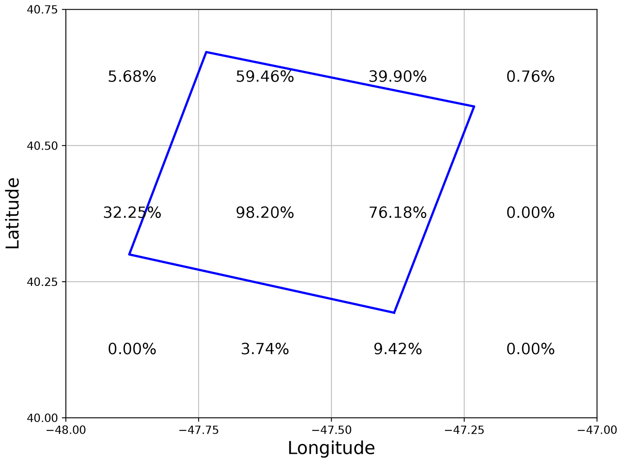
Figure 1 A GOME-2A ground pixel (blue) overlaid on a 0.25^∘ × 0.25^∘ latitude–longitude grid (grey). The percentage of overlap (weighting) for each grid box is indicated.

Several gridding routines have been developed to create global and regional maps of the trace gas distribution, e.g. Wenig et al. (2008), Chan et al. (2012), and Kuhlmann et al. (2014). These gridding algorithms typically assume that measurement values are constant within the satellite pixel boundaries. This assumption is considered sufficient for creating global maps. A more sophisticated approach uses a parabolic spline method to interpolate adjacent satellite pixels to create high-resolution (e.g. 1 km × 1 km) regional maps (Kuhlmann et al., 2014). As GOME-2 ground pixel size is relatively large, a significant grid effect would be induced by assigning each GOME-2 measurement to a single grid cell based on their centre coordinates of the GOME-2 ground pixel without taking into account the pixel geometry and extension. Therefore, the gridding process considers the overlapping area of the GOME-2 ground pixel and the latitude–longitude grid. For grid cells partially overlapping with the satellite pixel, the percentage of overlap (a satellite pixel fully covering the entire grid cell is considered 100 % overlap) is calculated and used as weighting for the calculation of the mean value, uncertainty, and standard deviation. Figure 1 shows an example of the calculation of the weighting (percentage of overlap) for grid boxes overlapping with a GOME-2A ground pixel. The gridded columns can be expressed as Eq. (1).

$$\begin{array}{}\text{(1)}& {\mathrm{VCD}}_{\mathrm{g}}={\displaystyle \frac{{\sum }_{i=\mathrm{1}}^n{\mathrm{VCD}}_{\mathrm{i}}\times w_{\mathrm{i}}}{{\sum }_{i=\mathrm{1}}^n{w}_{\mathrm{i}}}},\end{array}$$

where VCD_g is the gridded trace gas column, while VCD_i represents each individual satellite measurement (partly) overlapping with the grid cell. The weighting is denoted as w, which is the percentage of the grid cell covered by the satellite pixel. The weighting or the number of observations is also included in the level-3 product. The uncertainty of gridded columns can be expressed as Eq. (2).

$$\begin{array}{}\text{(2)}& E_{\mathrm{g}}=\sqrt{{\displaystyle \frac{{\sum }_{i=\mathrm{1}}^n{E}_{\mathrm{i}}^{\mathrm{2}}\times w_{\mathrm{i}}^{\mathrm{2}}}{{\sum }_{i=\mathrm{1}}^n{w}_{\mathrm{i}}^{\mathrm{2}}}}},\end{array}$$

where E_g is the uncertainty of the gridded trace gas column, while E_i represents the uncertainty of each individual measurement. The standard deviation of gridded columns can be expressed as Eq. (3).

$$\begin{array}{}\text{(3)}& {\mathit{\sigma }}_{\mathrm{g}}=\sqrt{{\displaystyle \frac{{\sum }_{i=\mathrm{1}}^n{\mathrm{VCD}}_{\mathrm{i}}^{\mathrm{2}}\times w_{\mathrm{i}}^{\mathrm{2}}}{{\sum }_{i=\mathrm{1}}^n{w}_{\mathrm{i}}^{\mathrm{2}}}}-{\left({\displaystyle \frac{{\sum }_{i=\mathrm{1}}^n{\mathrm{VCD}}_{\mathrm{i}}\times w_{\mathrm{i}}}{{\sum }_{i=\mathrm{1}}^n{w}_{\mathrm{i}}}}\right)}^{\mathrm{2}}},\end{array}$$

where σ_g is the standard deviation of the gridded trace gas column.

3.2 Sampling resolution

The processing of GOME-2 level-3 data requires binning of the level-2 data onto a regular two-dimensional latitude–longitude grid. The selection of an appropriate resolution of the latitude–longitude grid is essential for the production of the level-3 products. On the one hand, it is important to preserve the original spatial features captured in the level-2 data with higher spatial resolution, but on the other hand, it is necessary to keep the data files to a reasonable size to be user-friendly.

Figure 2 GOME-2A observations of total column O₃ (first row), total column NO₂ (second row), tropospheric column NO₂ (third row), total column water vapour (fourth row), total column BrO (fifth row), total column HCHO (sixth row), and total column SO₂ (seventh row). Data are shown at the original instrument resolution (first column from the left), gridded with 0.1^∘ × 0.1^∘ resolution (second column from the left), 0.25^∘ × 0.25^∘ resolution (third column from the left), and 0.5^∘ × 0.5^∘ resolution (column on the right). GOME-2A observations on 15 July 2014 over North China are shown. Missing data are mainly due to cloudiness.

To select the best spatial resolution for the level-3 product, we have analysed the binning results with various resolutions, i.e. 0.1^∘ × 0.1^∘, 0.25^∘ × 0.25^∘, and 0.5^∘ × 0.5^∘. Figure 2 shows GOME-2A data of each trace gas species gridded at different resolutions and level-2 data at the original instrument resolution for an orbit over North China on 15 July 2014. Missing data are mainly due to filtering of cloudy pixels and other low-quality observations. GOME-2A data are shown due to their highest spatial resolution among all three GOME-2 instruments (GOME-2A: 40 km × 40 km after 15 July 2013, GOME-2B and GOME-2C: 40 km × 80 km). We looked into the spatial smoothing/averaging effect over North China, as this region is expected to show strong spatial gradients of tropospheric pollutants, i.e. NO₂. Data at all four resolutions show very similar spatial structures. The absolute values of level-3 data are also consistent with the level-2 product. The results show that gridding GOME-2 data with a higher spatial resolution (i.e. 0.1^∘ × 0.1^∘) better preserves the original GOME-2 instrument footprint, while a rather strong smoothing/averaging effect is observed from data gridded with a lower spatial resolution (i.e. 0.5^∘ × 0.5^∘). Although gridded data with a 0.25^∘ × 0.25^∘ resolution show some smoothing/averaging effects, they still capture the spatial variations reasonably well.

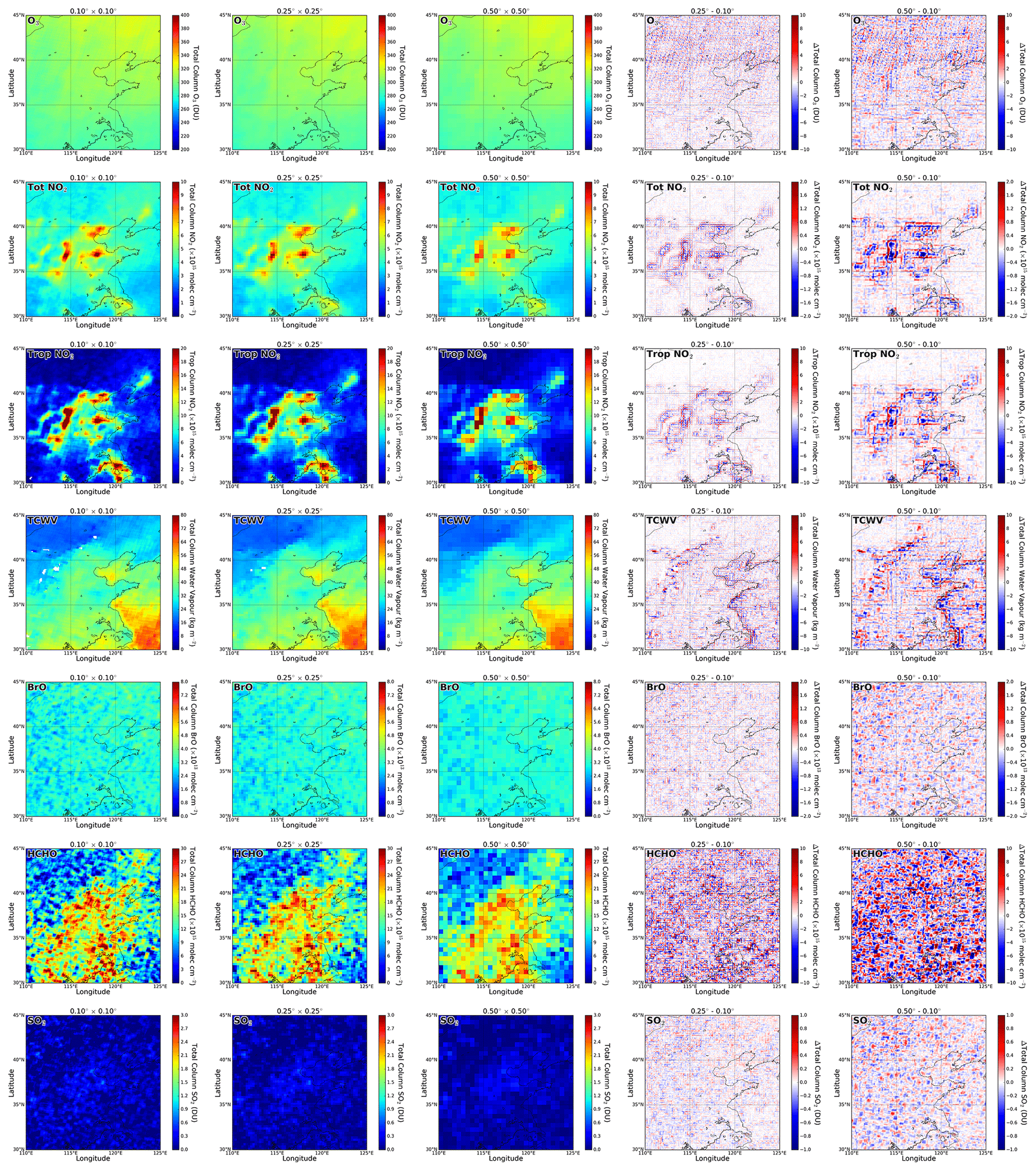
Figure 3 Monthly averaged GOME-2A observations of total column O₃ (first row), total column NO₂ (second row), tropospheric column NO₂ (third row), total column water (fourth row), vapour total column BrO (fifth row), total column HCHO (sixth row), and total column SO₂ (seventh row) over North China in July 2014. Gridded data with 0.1^∘ × 0.1^∘ resolution (first column from the left), 0.25^∘ × 0.25^∘ resolution (second column from the left), and 0.5^∘ × 0.5^∘ resolution (third column from the left) are shown. Differences between 0.1^∘, 0.25^∘, and 0.5^∘ are also shown for reference.

Figure 3 shows the monthly averaged GOME-2A data of each trace gas species gridded at different resolutions over North China in July 2014. Differences between data gridded with different resolutions are also shown for reference. Data gridded at all three resolutions show very similar spatial structures. Hotspots of anthropogenic pollutants, i.e. tropospheric NO₂, can be clearly observed from the monthly averaged data. Species with major contributions from natural sources, e.g. O₃ and water vapour, show a rather smooth appearance. Despite the fact that large numbers of observations are included in the monthly averaging process, species with lower signal-to-noise ratios, e.g. HCHO and SO₂, still show rather high background noise. This is mainly due to the low column density and absorption of these species. This effect is as expected more significant for data gridded at a higher spatial resolution, i.e. 0.1^∘ × 0.1^∘, due to less spatial averaging. Traces of the satellite footprints can still be seen in the 0.1^∘ × 0.1^∘-resolution monthly averaged data, while the satellite footprints are much less significant in the 0.25^∘ × 0.25^∘- and 0.5^∘ × 0.5^∘-resolution data. The differential plots between data gridded with 0.1^∘ × 0.1^∘ and 0.25^∘ × 0.25^∘ resolution in general show only very small differences. Slightly larger discrepancies mainly appear over pollution hotspots, i.e. for tropospheric NO₂. In contrast, data at 0.5^∘ × 0.5^∘ resolution show much bigger differences from 0.1^∘ × 0.1^∘-resolution data. Compared to 0.25^∘ × 0.25^∘-resolution data, 0.5^∘ × 0.5^∘-resolution data show 2 to 4 times higher underestimation of tropospheric NO₂ columns over pollution hotspots. The comparison of GOME-2 data gridded at different resolutions indicates that 0.25^∘ × 0.25^∘ resolution is a balance to preserve the satellite resolution (GOME-2A: 40 km × 40 km, GOME-2B and GOME-2C: 40 km × 80 km) while capturing the strong spatial variations for most of the tropospheric gases, i.e. NO₂, water vapour, and HCHO. In addition, the data file size of level-3 products with 0.1^∘ × 0.1^∘ resolution is about 6 times larger than that of 0.25^∘ × 0.25^∘, while the information content does not show a significant difference, especially for monthly products. Therefore, we concluded that 0.25^∘ × 0.25^∘ resolution is a suitable choice for GOME-2 level-3 products.

3.3 Verification and validation methods

The GOME-2 level-3 products are generated from the level-2 data sets which have already been fully validated (see the validation reports in https://acsaf.org/valreps.php, last access: 15 March 2023). Therefore, the verification and validation of the GOME-2 level-3 product mainly focus on two major aspects, the consistency among the three GOME-2 sensors and the comparison to reference ground-based measurements. Each GOME-2 level-3 product is compared to different reference ground-based measurements, and information on the reference ground-based measurements used to validate GOME-2 level-3 products is listed in Table 3.

The comparison of GOME-2 level-3 data to reference ground-based measurements requires spatial and temporal matching of the two data sets. The following criteria are applied to co-locate the GOME-2 level-3 products and ground-based reference data sets.

• The grid cells of the level-3 GOME-2 products covering the ground-based measurement site are paired with the daily/monthly ground-based measurements.

• For ground-based Brewer, MAX-DOAS, sun-photometer, and Pandora measurements, they are temporally averaged around the GOME-2 overpass time from 08:30 to 10:30 (local time).

• For ZSL-DOAS measurements, morning twilight period measurement is used for comparison.

After co-locating the GOME-2 and ground-based data sets, we compare the GOME-2 level-3 products to reference ground-based data sets through a scatter plot and histogram of the differences and sort the differences/biases by year, latitude band, or measurement site as a box plot and time series to investigate the systematic bias/error.

4 GOME-2 level-3 products

The GOME-2 level-3 products are at two different temporal resolutions, daily and monthly. Both daily and monthly level-3 products consist of gridded trace gas columns and other auxiliary parameters, i.e. cloud, surface, and statistical parameters. The level-3 products are separated for each species (i.e. O₃, NO₂, water vapour, BrO, HCHO, and SO₂) and each GOME-2 instrument (i.e. GOME-2A, GOME-2B, and GOME-2C). All products are at a spatial resolution of 0.25^∘ × 0.25^∘, with coordinates ranging from 180^∘ W to 180^∘ E in longitude and from 90^∘ S to 90^∘ N in latitude (720 (latitude) × 1440 (longitude) grid cell). The data are organized into a user-friendly and self-describing NetCDF-4 (Network Common Data Form) format, based upon the instrument/platform (GOME-2A/Metop-A, GOME-2B/Metop-B, or GOME-2C/Metop-C) and the temporal period of collection (daily or monthly data set).

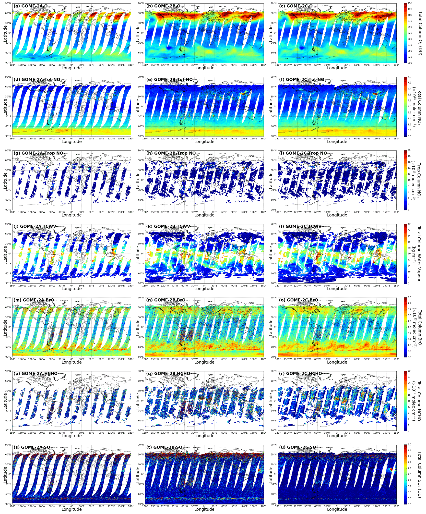
Figure 4 Daily level-3 product of GOME-2A (first column), GOME-2B (second column), and GOME-2C (third column) for 15 January 2020. Total column O₃ (first row), total column NO₂ (second row), tropospheric column NO₂ (third row), total column water vapour (fourth row), total column BrO (fifth row), total column HCHO (sixth row), and total column SO₂ (seventh row) are shown.

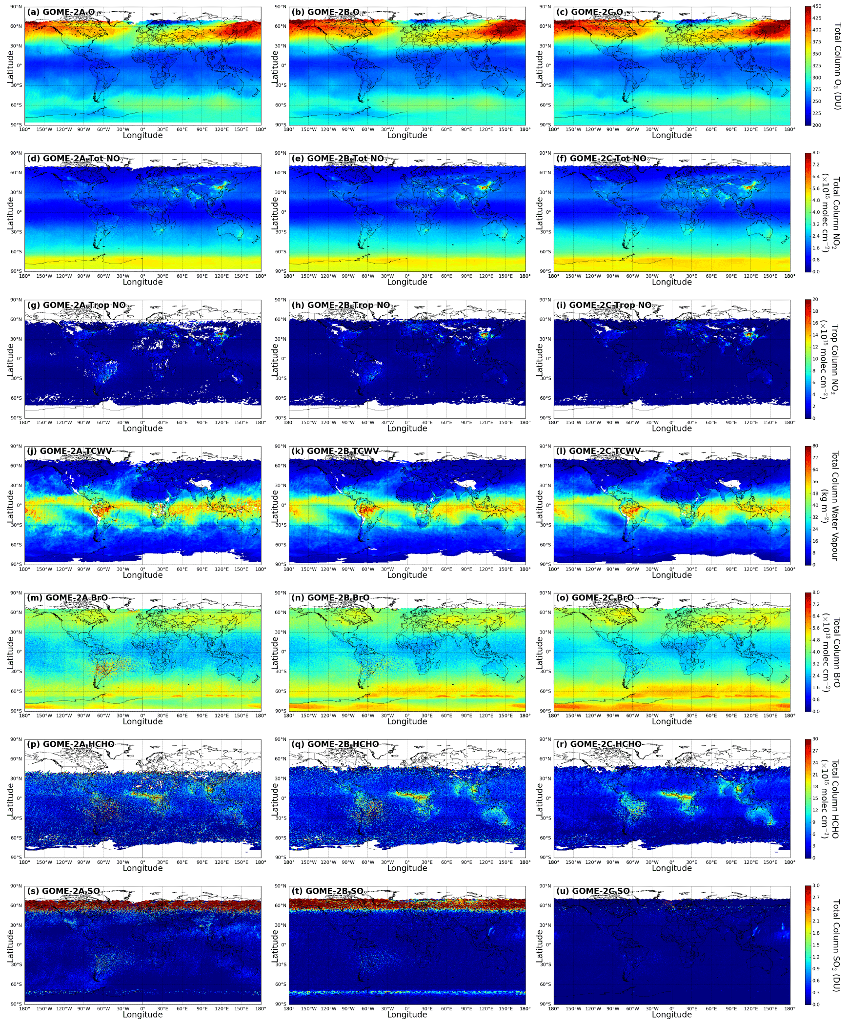
Figure 5 Monthly level-3 product of GOME-2A (first column), GOME-2B (second column), and GOME-2C (third column) for January 2020. Total column O₃ (first row), total column NO₂ (second row), tropospheric column NO₂ (third row), total column water vapour (fourth row), total column BrO (fifth row), total column HCHO (sixth row), and total column SO₂ (seventh row) are shown.

Figure 4 shows examples of the daily level-3 products for all trace gases and all GOME-2 instruments, while examples of monthly level-3 data are shown in Fig. 5. Missing data are mainly due to filtering of low-quality data, e.g. cloud contamination, high solar zenith angle, and high spectral fit residual. The spatial coverage of the GOME-2A daily product is different from GOME-2B and GOME-2C due to the improvement in spatial resolution after it went into tandem operation with GOME-2B in July 2013. The noise levels of monthly GOME-2A data are significantly higher than those of GOME-2B and GOME-2C. This is mainly related to less spatial averaging and instrument aging. This effect is particularly obvious for species with a lower signal-to-noise ratio, e.g. HCHO and SO₂. In addition, the stripe pattern is also more significant for GOME-2A, e.g. the water vapour product, due to the narrower swath width of GOME-2A measurements.

Figure 6 Derived measurement errors in the daily level-3 product of GOME-2A (first column), GOME-2B (second column), and GOME-2C (third column) for 15 January 2020. Measurement errors of total column O₃ (first row), total column NO₂ (second row), tropospheric column NO₂ (third row), total column water vapour (fourth row), total column BrO (fifth row), total column HCHO (sixth row), and total column SO₂ (seventh row) are shown.

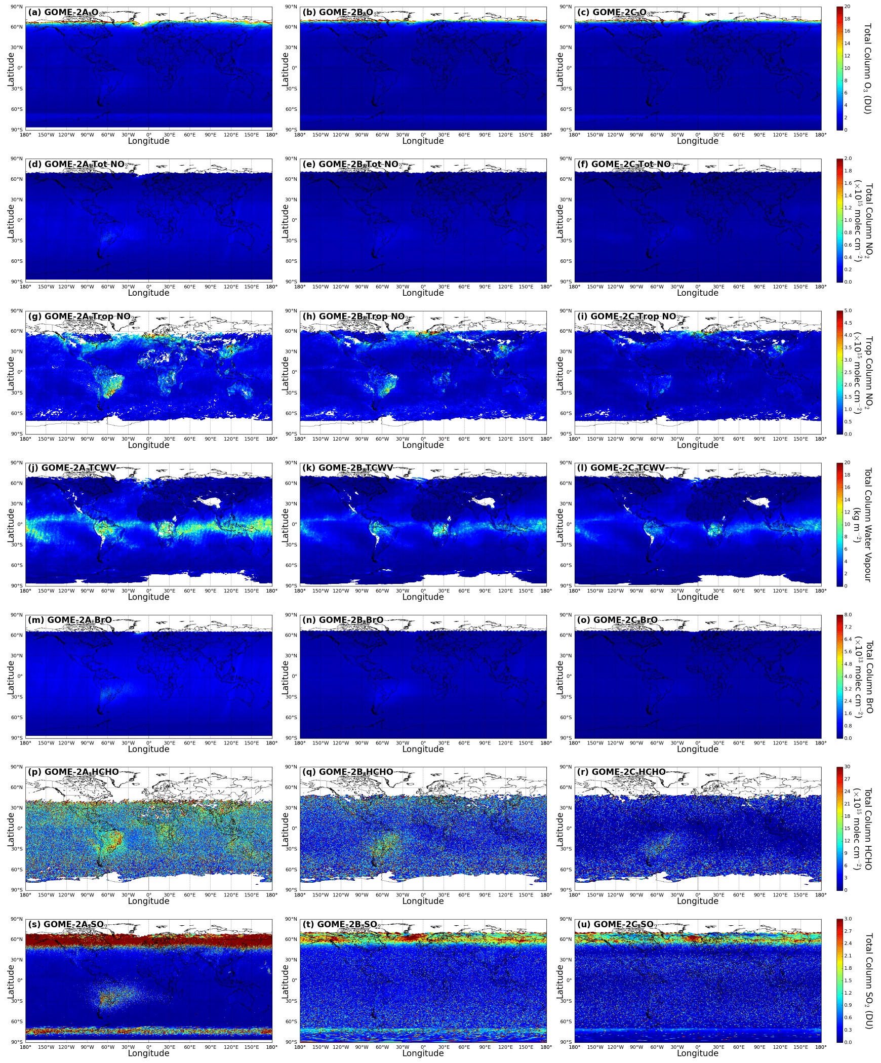
Figure 7 Derived measurement errors in the monthly level-3 product of GOME-2A (first column), GOME-2B (second column), and GOME-2C (third column) for January 2020. Measurement errors of total column O₃ (first row), total column NO₂ (second row), tropospheric column NO₂ (third row), total column water vapour (fourth row), total column BrO (fifth row), total column HCHO (sixth row), and total column SO₂ (seventh row) are shown.

Figures 6 and 7 show examples of derived measurement errors in the daily and monthly level-3 products for all trace gases and all GOME-2 instruments. The measurement errors are in general related to the instrument noise, a priori assumption in the AMF calculations, and cloud effect and climatological input parameters, such as surface albedo and pressure profile. Some of the terms are multiplicable, such as AMFs, and therefore they are higher where the columns are higher. For measurement with a lower signal-to-noise ratio, such as HCHO and SO₂, the measurement errors increase significantly in the polar regions, where the radiance intensities are low, as they are observed with higher solar zenith angles. The inclusion of measurement error in the level-3 products provides addition information on the measurement accuracy, and users can use it as an indicator to make additional filtering of the data.

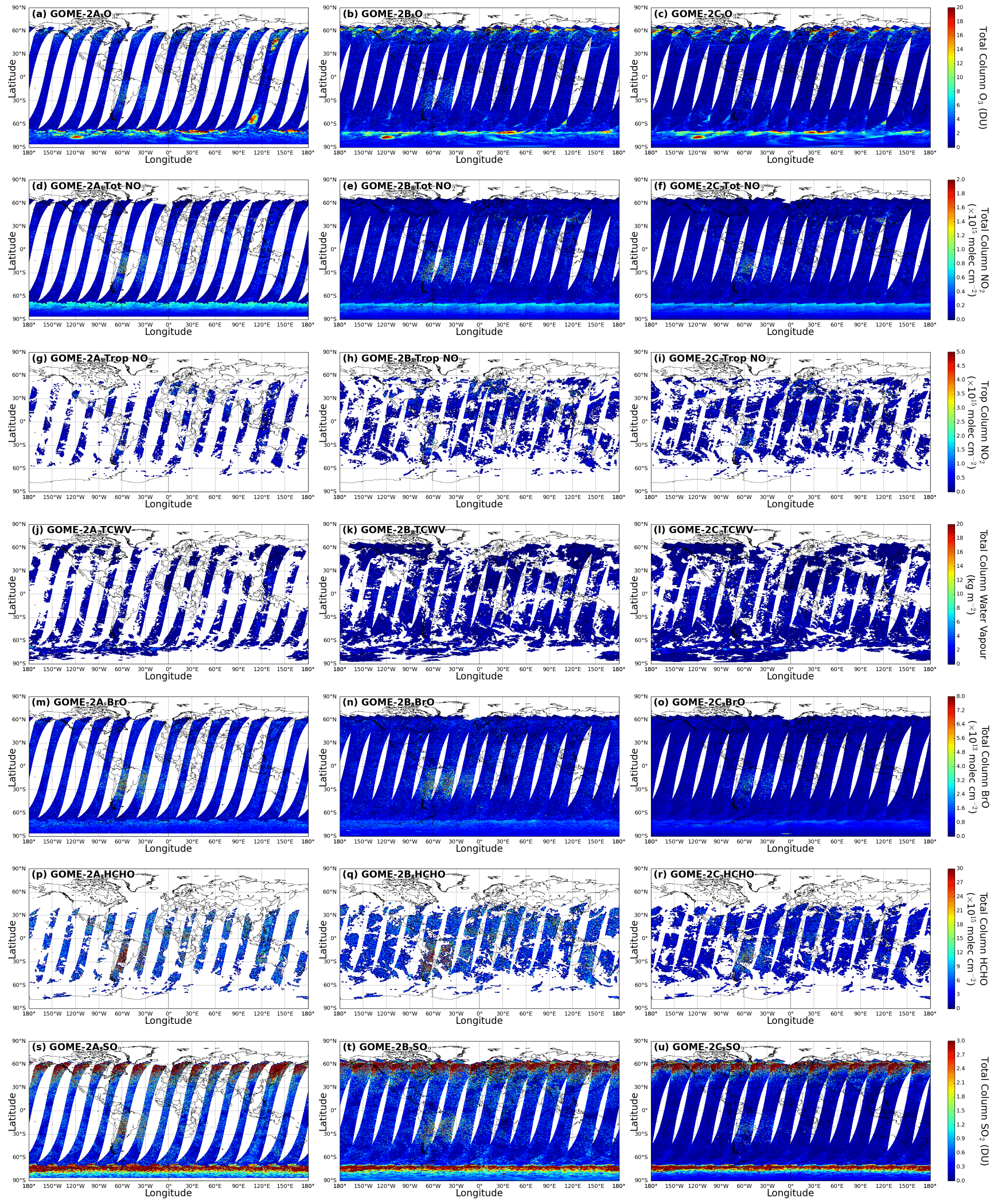
Figure 8 Derived standard deviation in the daily level-3 product of GOME-2A (first column), GOME-2B (second column), and GOME-2C (third column) for 15 January 2020. Standard deviation of total column O₃ (first row), total column NO₂ (second row), tropospheric column NO₂ (third row), total column water vapour (fourth row), total column BrO (fifth row), total column HCHO (sixth row), and total column SO₂ (seventh row) are shown.

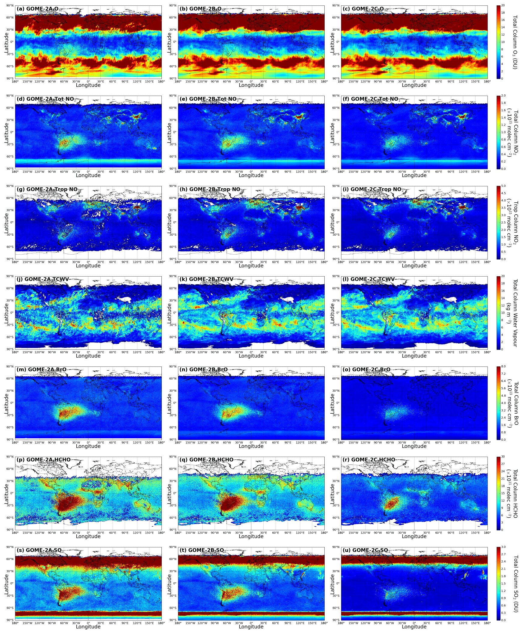
Figure 9 Derived standard deviation in the monthly level-3 product of GOME-2A (first column), GOME-2B (second column), and GOME-2C (third column) for January 2020. Standard deviation of total column O₃ (first row), total column NO₂ (second row), tropospheric column NO₂ (third row), total column water vapour (fourth row), total column BrO (fifth row), total column HCHO (sixth row), and total column SO₂ (seventh row) are shown.

Figures 8 and 9 show examples of the standard deviation in the daily and monthly level-3 products for all trace gases and all GOME-2 instruments. The standard deviation in most areas (except the polar regions) in the daily products is expected to be close to 0, as there is only overlap with neighbouring pixels measured at roughly the same time of the day, while the standard deviation over the polar regions is expected to be higher as there are multiple measurements at different times of the day. The standard deviation in the monthly products reflects both the instrument/measurement noise and the natural variability. Higher standard deviations of SO₂ columns over the polar regions are related to the low signal-to-noise ratio for observations taken with high solar zenith angles. In addition, the standard deviations of NO₂, BrO, HCHO, and SO₂ are higher over South America, mainly due to high cloudiness, while the standard deviations of O₃ and water vapour columns are mainly driven by their natural variability. The standard deviation in the level-3 products provides additional information on the measurement precision and natural variability. Depending on the propose, users can use it to filter the data or study the variability.

5 Validation

In this section, we present validation results of the GOME-2 level-3 products. The GOME-2 level-3 products are first examined with respect to their cross-sensor consistency. In addition, level-3 products of each trace gas are compared to ground-based observations for validation.

5.1 Cross-sensor consistency

5.1.1 Average and bias

Figure 10 shows the global monthly mean time series of (a) total column O₃, (b) total column NO₂, (c) tropospheric column NO₂, (d) total column water vapour, (e) total column BrO, (f) total column HCHO, and (g) total column SO₂ for GOME-2A, GOME-2B, and GOME-2C. The error bars represent the 1σ standard deviation of variation. All species except for SO₂ show pronounced seasonal variation patterns. The seasonal patterns are related to the natural variability and the variation of the coverage area of the GOME-2 measurements.

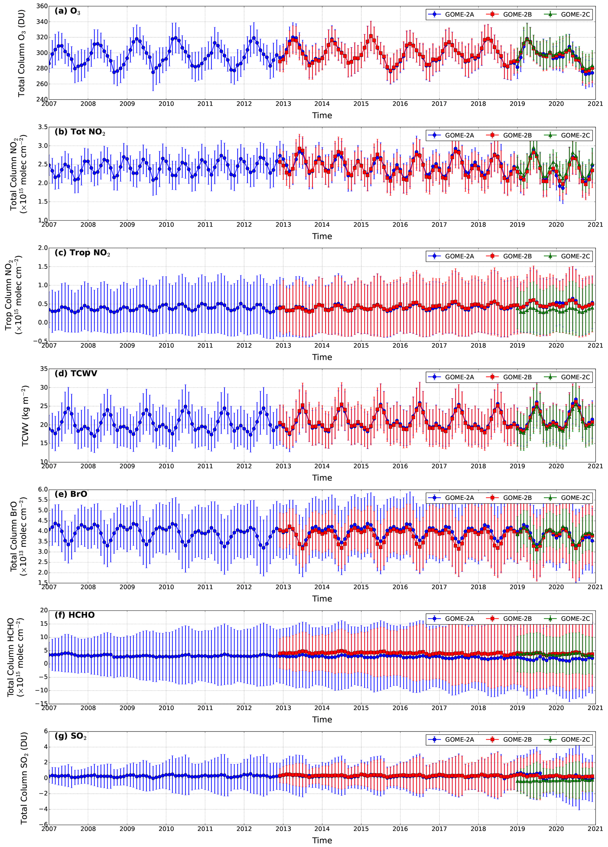
Figure 10 Time series of global monthly mean (a) total column O₃, (b) total column NO₂, (c) tropospheric column NO₂, (d) total column water vapour, (e) total column BrO, (f) total column HCHO, and (g) total column SO₂ for GOME-2A (blue lines), GOME-2B (red lines), and GOME-2C (green lines). The error bars represent the 1σ standard deviation variation.

The global monthly mean total column O₃ time series of GOME-2A, GOME-2B, and GOME-2C mostly overlap with each other, indicating the good agreement among the three sensors. However, GOME-2C reports a slightly higher (2–3 DU) value compared to GOME-2A and GOME-2B. This is likely related to the small difference in instrument characteristic, e.g. scan angle dependency and polarization sensitivity.

For total column NO₂, observations from GOME-2A and GOME-2B show very good consistency, while GOME-2C data are about 1.2 × 10¹⁴ molec cm⁻² higher than those of GOME-2A and GOME-2B. Tropospheric column NO₂ from GOME-2A and GOME-2B is also in good agreement. However, GOME-2C observations are about 1.5 × 10¹⁴ molec cm⁻² lower than GOME-2A and GOME-2B observations. The discrepancies in NO₂ observations are likely related to the different processor versions (GDP 4.8 for GOME-2A and GOME-2B and GDP 4.9 for GOME-2C). The spectral-fitting band of NO₂ is slightly different in different processor versions (see Sect. 2.2.2). A previous validation study shows that the NO₂ slant columns retrieved from GOME-2C observations are slightly higher than those of GOME-2B (Pinardi et al., 2019), indicating the impact of the different spectral-fitting bands on the NO₂ retrieval. In addition, the positive bias in the GOME-2C total column NO₂ shows an impact on the tropospheric columns in the stratospheric and tropospheric separation process (Pinardi et al., 2019) and results in the discrepancies in the tropospheric columns.

Total column water vapour measurements from all three GOME-2 sensors also show very good consistency, with a bias smaller than 1 kg m⁻².

For BrO observations, GOME-2B measurements show a negative bias of ∼ 1.0–1.5 × 10¹² molec cm⁻² compared to GOME-2A and GOME-2C. The discrepancies are partly related to the difference in the scanning swath width and the scan angle dependency (Merlaud et al., 2020). The impact of scan angle dependency on BrO measurements is more significant for GOME-2C compared to GOME-2B, which is likely linked to the polarization sensitivity of the GOME-2C instrument (Merlaud et al., 2020).

GOME-2A observations of total column HCHO are in general 1.5–1.9 × 10¹² molec cm⁻² lower than GOME-2B and GOME-2C measurements. Lower HCHO columns are observed by GOME-2A over the Amazon, central Africa, Southeast Asia, and Australia (see Fig. 5), thus resulting in slightly lower global averages. Similarly to BrO measurements, the scan angle dependency issue is also reported as significant for GOME-2C HCHO observations (Pinardi et al., 2020b). The scan angle dependency effect can also be seen in the BrO and HCHO daily level-3 product.

Total column SO₂ observations from GOME-2C are in general 0.5 DU lower than GOME-2A and GOME-2B, resulting in a slightly negative global average. The higher global average of SO₂ observed by GOME-2A and GOME-2B is related to the extreme values taken with a high solar zenith angle and thus low signal-to-noise ratio (see Figs. 4 and 5), while this effect is much less significant for GOME-2C. The overall bias and root mean square error among the GOME-2 sensors for each product are summarized in Table 2.

Table 2 Bias and root mean square error of trace gas columns among the three GOME-2 sensors.

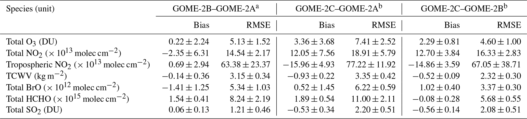
^a For the period from 2013 to 2021. ^b For the period from 2019 to 2021.

Table 3 Summary of the GOME-2 level-3 data comparison to ground-based measurements.

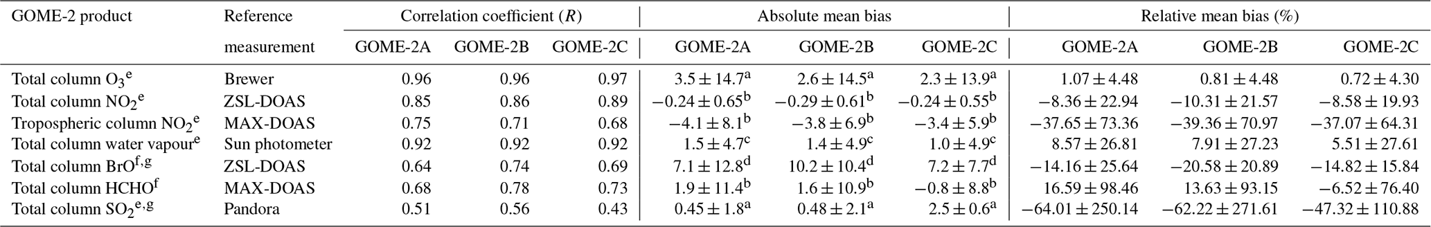
^a Unit DU, ^b unit 10¹⁵ molec cm⁻², ^c unit kg m⁻², and ^d unit 10¹² molec cm⁻². ^e Regression is computed based on daily data, and ^f regression is computed based on monthly data. ^g Based on comparison at a single location. All biases are calculated based on daily data.

5.1.2 Zonal average

Each GOME-2 monthly averaged level-3 product derived from all three sensors is sorted by latitude and is plotted in Fig. 11.

Figure 11 Monthly zonal average of total column O₃ (first row), total column NO₂ (second row), tropospheric column NO₂ (third row), total column water vapour (fourth row), total column BrO (fifth row), total column HCHO (sixth row), and total column SO₂ (seventh row). Data from GOME-2A (first column from the left), GOME-2B (second column from the left), and GOME-2C (third column from the left) are shown.

All three GOME-2 sensors show consistent zonal and seasonal O₃ patterns. Higher O₃ columns are observed over high latitudes, and lower values are found over the tropics. Total column O₃ over the Arctic shows a peak in February to March and a minimum in August to October, while Antarctica displays a reverted seasonal pattern.

Both total and tropospheric column NO₂ from all three GOME-2 sensors shows good zonal and seasonal consistency. Elevated total column NO₂ is observed in the polar regions during the warm months. This seasonal pattern is attributed to the stratospheric variation of NO₂. Compared to total column NO₂, tropospheric column NO₂ shows a very different zonal and seasonal pattern. Tropospheric NO₂ is mostly concentrated at the mid-latitudes of the Northern Hemisphere. This is because most of the population lives in this part of the world, and thus higher emissions occur at this latitude band. Tropospheric NO₂ at mid-latitudes also shows a seasonal pattern with higher values over winter, which is related to higher energy consumption and a longer atmospheric lifetime of NO₂ during the cold months. A significant increasing trend of tropospheric NO₂ was observed by GOME-2A and GOME-2B over the sub-tropics and mid-latitudes of the Southern Hemisphere in recent years (see Fig. 11g and h). GOME-2C observed a much less significant enhancement of tropospheric NO₂ in the Southern Hemisphere, which leads to lower global-average tropospheric NO₂ measured by GOME-2C. This discrepancy is likely related to the difference in retrieval wavelength and the subsequent stratosphere and troposphere separation process.

Total column water vapour observations from all three GOME-2 sensors show consistent zonal and seasonal patterns, with higher values in the tropics and lower values at high latitudes. Total column water vapour is also higher during the warm months of the corresponding hemisphere.

All three GOME-2 sensors also show very similar zonal and seasonal patterns of total column BrO. However, GOME-2A total column BrO observations from 2014 to 2019 are slightly higher than those of GOME-2B at all latitude bands and result in a small bias of 1.41 × 10¹² molec cm⁻². However, when we look into the data from 2020 to 2021, the bias is smaller and results in a smaller bias of 0.52 × 10¹² molec cm⁻² with GOME-2C observations.

The total column HCHO from all three GOME-2 sensors shows higher values over the tropics and sub-tropics, while lower values appear at higher latitudes. Both GOME-2A and GOME-2B measurements show a significant decreasing trend of HCHO in the Southern Hemisphere. However, GOME-2A measurements are significantly lower than GOME-2B and GOME-2C, resulting in biases of −1.54 and −1.89 × 10¹⁵ molec cm⁻² when compared to GOME-2B and GOME-2C observations. The discrepancy is related to the underestimation over HCHO-rich regions, e.g. the Amazon, Australia, Southeast Asia, China, and North America (see Fig. 5). This bias is probably related to the background correction process.

Total column SO₂ observations from all three GOME-2 sensors show very low SO₂ levels (very close to 0) around the globe, as expected. However, GOME-2A and GOME-2B measurements show significantly higher noise for measurement with a high solar zenith angle and result in a small overestimation under these extreme observation geometries, while this effect is much less significant for GOME-2C. Therefore, GOME-2C observations are in general about 0.5 DU lower than GOME-2A and GOME-2B. GOME-2A measurement is also about 0.5 DU higher in general compared to the years before and after.

5.2 Comparison to ground-based observations

In this section, all GOME-2 level-3 products are compared to the corresponding reference ground-based observations. We look into the scatter plot and histogram of the differences and sort the differences/biases by year, latitude band, or measurement site as a box plot and time series between GOME-2 and reference data sets to investigate the systematic bias/error.

5.2.1 Total column ozone

Daily and monthly GOME-2 level-3 total column ozone is compared to the co-located Brewer observations. Figure 12 shows the density scatter plots for the comparison of total column ozone between GOME-2 and ground-based Brewer observations. Comparisons of GOME-2A, GOME-2B, and GOME2-C data are shown in Fig. 12a, b, and c, respectively. Monthly data are also shown as black dots. Histograms of the differences between GOME-2 and Brewer observations are shown in Fig. 12d. Scatter plots show that GOME-2 monthly data are well in line with the daily data, and the agreement between GOME-2 and Brewer is in general very good, with a Pearson correlation coefficient (R) of ∼ 0.96 for all three GOME-2 sensors. The slopes of the total least-squares regression for the comparisons of all three instruments are very close to 1 (1.03 for GOME-2A, 1.01 for GOME-2B, and 0.99 for GOME-2C). The offsets of the total least-squares regression range between −5.1 and 4.3 DU. In general, the GOME-2 data sets show a small positive bias of 2.3 to 3.5 DU (0.72 %–1.07 %) compared to Brewer observations, with a standard deviation of 13.9 to 14.7 DU (4.03 %–4.48 %). The bias between all three GOME-2 sensors and the ground-based Brewer observations is below 1 %, which is within the uncertainty of Brewer measurements (Kerr et al., 1988) and fulfils the product requirements.

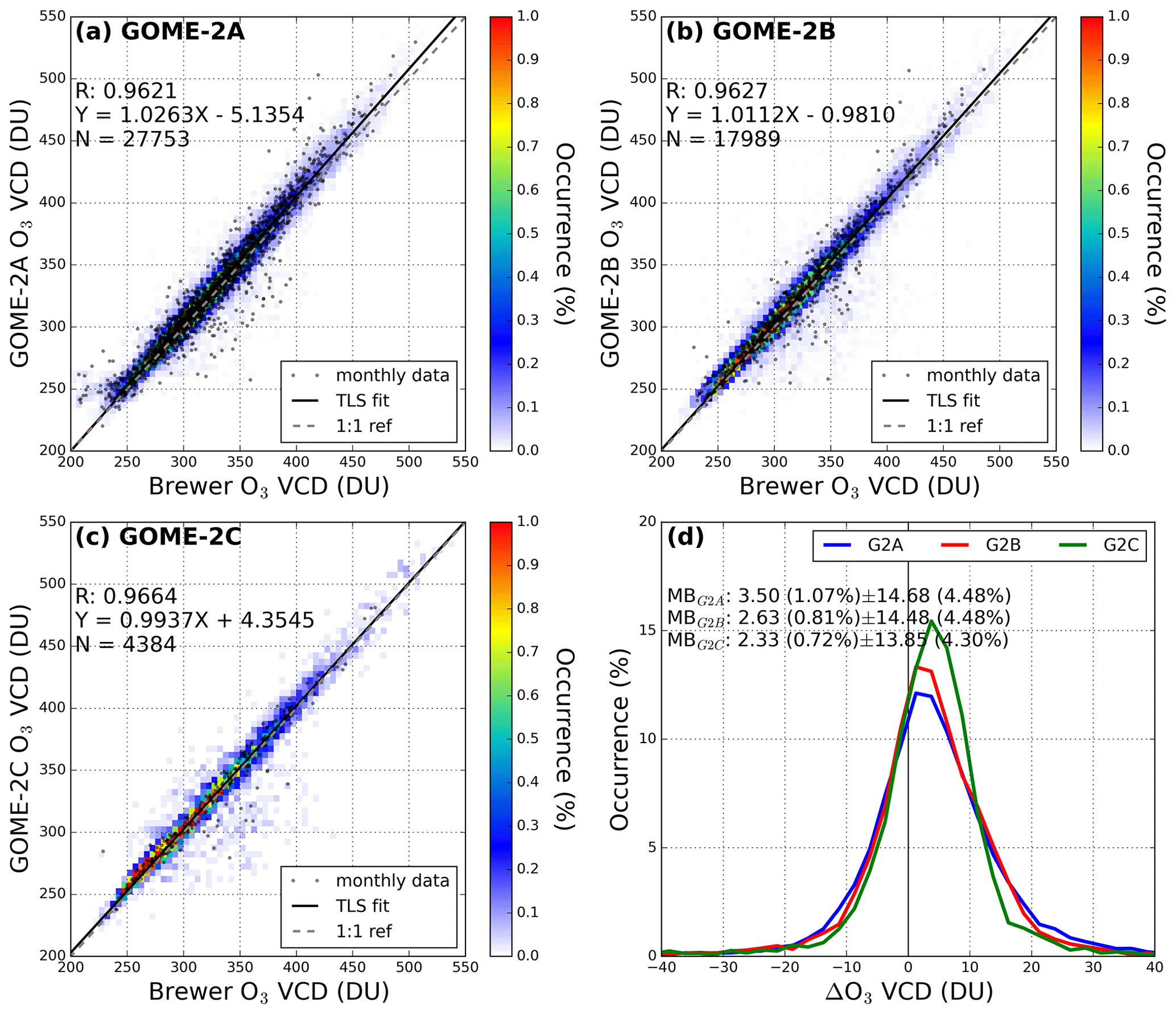
Figure 12 Comparison of daily and monthly total column O₃ measured by the ground-based Brewer instruments to (a) GOME-2A, (b) GOME-2B, and (c) GOME-2C. Histograms of the differences in total column O₃ between GOME-2 and Brewer observations are shown in panel (d). Co-located daily and monthly averaged data are used in the comparison. Total least-squares regression is based on daily data.

Figure 13 Comparison of total column O₃ between ground-based Brewer instruments and GOME-2 observations. Data are sorted by year in panel (a) and latitude band in panel (b).

Figure 13 shows box plots of the differences in total column ozone between the GOME-2 level-3 product and the co-located Brewer measurements. GOME-2 data are sorted by the measurement year (Fig. 13a) and latitude band (Fig. 13b). The box plot for the Southern Hemisphere is mostly empty due to an insufficient number of ground-based observations. The mean differences between GOME-2 and Brewer observations are within 5 DU for most of the years. However, we observed that there are years with a positive bias and some years with a negative bias. This is mostly related to the availability of ground-based data at different measurement sites, as some sites are biased high/low, and it will affect the statistic if they are not available for some years. On the other hand, the latitude-dependent analysis shows that GOME-2 observations are consistently higher than the ground-based Brewer measurements in the Northern Hemisphere and result in a positive bias of 2.3 to 3.5 DU on average. In addition, GOME-2C observations are about 2–3 DU higher than GOME-2A and GOME-2B, which is likely related to the instrumental issues which have been mentioned in Sect. 5.1.1.

5.2.2 Total column NO₂

Daily and monthly GOME-2 level-3 total column NO₂ is compared to the co-located ZSL-DOAS observations. Figure 14 shows the density scatter plots for the comparison of total column NO₂ between GOME-2 and ground-based ZSL-DOAS observations. Comparisons of GOME-2A, GOME-2B, and GOME-2C data are shown in Fig. 14a, b, and c, respectively. Monthly data are also shown as black dots. Histograms of the differences between GOME-2 and ZSL-DOAS observations are shown in Fig. 14d. Scatter plots show that GOME-2 monthly data are well in line with the daily data. GOME-2 level-3 total column NO₂ in general agrees well with ZSL-DOAS observations, with a Pearson correlation coefficient (R) of 0.85 to 0.88. However, GOME-2 observations are in general slightly lower than ZSL-DOAS observations. The slopes of the total least-squares fit for the comparisons of all three instruments vary from 0.84 to 0.88, with offsets ranging from 0.05 to 0.19 × 10¹⁵ molec cm⁻². Overall, the GOME-2 level-3 total NO₂ products are biased low by 0.24–0.29 × 10¹⁵ molec cm⁻² (8 %–10 %) compared to ground-based ZSL-DOAS measurements. Considering that the uncertainty of satellite and ground-based measurements is about 10 %, the agreement between the two data sets is very satisfactory.

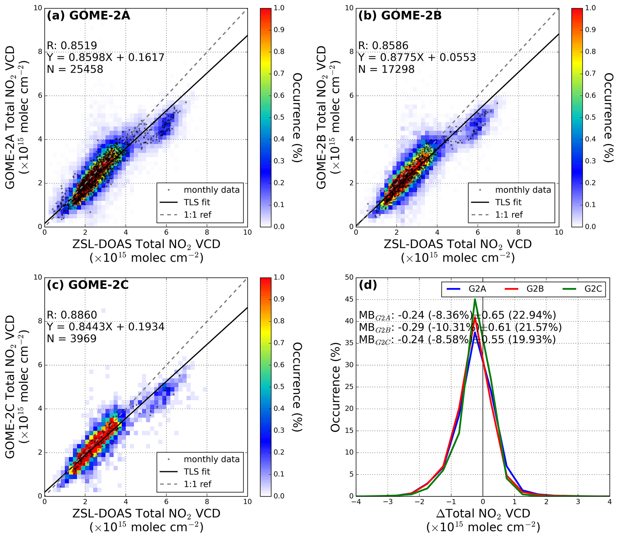
Figure 14 Comparison of daily and monthly total column NO₂ measured by the ground-based ZSL-DOAS to (a) GOME-2A, (b) GOME-2B, and (c) GOME-2C. Histograms of the difference in total column NO₂ between GOME-2 and ZSL-DOAS observations are shown in panel (d). Co-located daily and monthly averaged data are used in the comparison. Total least-squares regression is based on daily data.

Figure 15 Time series of total column NO₂ measured by GOME-2A (blue), GOME-2B (green), GOME-2C (red), and ZSL-DOAS (black). Observations over (a) Dumont d'Urville, Antarctica, and (b) Sodankylä, Finland, are shown.

The scatter plots for all three instruments show a two-cluster characteristic. The major cluster of total column NO₂ below 4 × 10¹⁵ molec cm⁻² shows very good agreement between GOME-2 and ZSL-DOAS observations. The minor cluster at 5–6 × 10¹⁵ molec cm⁻² shows significant underestimation of the NO₂ column by 0.5–1.0 × 10¹⁵ molec cm⁻², which is related to the measurement over the polar regions. Figure 15 shows the time series of total column NO₂ measured at Dumont d'Urville, Antarctica, and Sodankylä, Finland. We observed that the total column NO₂ measured by GOME-2 is significantly lower than the ground-based ZSL-DOAS observations during summer months. This is because of the multiple overpasses over the polar regions during summertime. Therefore, GOME-2 level-3 data represent the real “daily average”, while ZSL-DOAS only captures the morning values. Due to the diurnal variation of NO₂, it is expected that ZSL-DOAS measurements in the morning will be higher than the daily averages. If we do not consider these two stations in the analysis, the minor cluster in the scatter plots would be removed. In addition, the underestimation would reduce to 0.13–0.21 × 10¹⁵ molec cm⁻² (5 %–7 %).

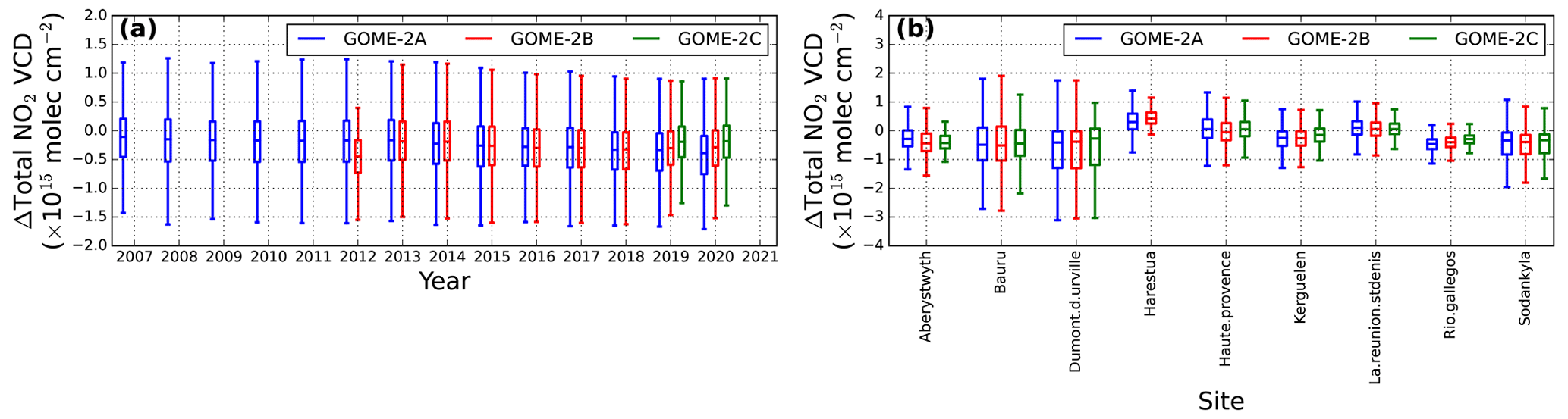
Figure 16 Comparison of total column NO₂ between ground-based ZSL-DOAS and GOME-2 observations. Data are sorted by year in panel (a) and measurement site in panel (b).

Figure 16 shows box plots of the differences in total column NO₂ between the GOME-2 level-3 product and co-located ZSL-DOAS measurements. Data are sorted by the measurement year (Fig. 16a) and measurement site (Fig. 16b). The mean differences between GOME-2 and ZSL-DOAS observations are within 0.3 × 10¹⁵ molec cm⁻² for most of the years, and this bias does not show significant temporal variation. Box plots for each measurement site show significant negative bias for some sites, i.e. Dumont d'Urville and Sodankylä. The reason for the negative bias has been explained above.

5.2.3 Tropospheric column NO₂

Daily and monthly GOME-2 level-3 tropospheric column NO₂ is compared to the co-located MAX-DOAS observations. Figure 17 shows the density scatter plots for the comparison of tropospheric column NO₂ between GOME-2 and ground-based MAX-DOAS observations. Comparisons of GOME-2A, GOME-2B, and GOME-2C data are shown in Fig. 17a, b, and c, respectively. Monthly data are also shown as black dots. Histograms of the differences between GOME-2 and MAX-DOAS observations are shown in Fig. 17d. GOME-2 monthly tropospheric NO₂ data are consistent with the daily data, and daily data show satisfactory correlation with ground-based MAX-DOAS observations, with a Pearson correlation coefficient (R) in the range of 0.68 to 0.75. However, GOME-2 tropospheric column NO₂ is in general ∼ 30 % lower than MAX-DOAS observations. The slopes of the total least-squares fit for the comparisons of all three instruments vary from 0.61 to 0.74, with offsets ranging from −1.03 to 0.18 × 10¹⁵ molec cm⁻². GOME-2 level-3 tropospheric NO₂ products on average show a negative bias of 3.38–4.14 × 10¹⁵ molec cm⁻² (37 %–39 %). The underestimation is mainly related to the a priori assigned too-low NO₂ concentration at the lower troposphere and a spatial averaging effect over large satellite pixels. A previous study shows that using a better a priori vertical profile in GOME-2 retrieval reduces the underestimation of GOME-2 measurement by 15 %–20 % (Liu et al., 2019). The spatial averaging effect has also been estimated to result in an underestimation of 15 %–25 % in tropospheric column NO₂ over pollution hotspots (Chen et al., 2009; Ma et al., 2013; Chan et al., 2020b; Pinardi et al., 2020a). Considering the sensitivity difference between satellite and ground-based MAX-DOAS measurements and the spatial averaging effect of large satellite footprints, the agreement between the two data sets is very satisfactory.

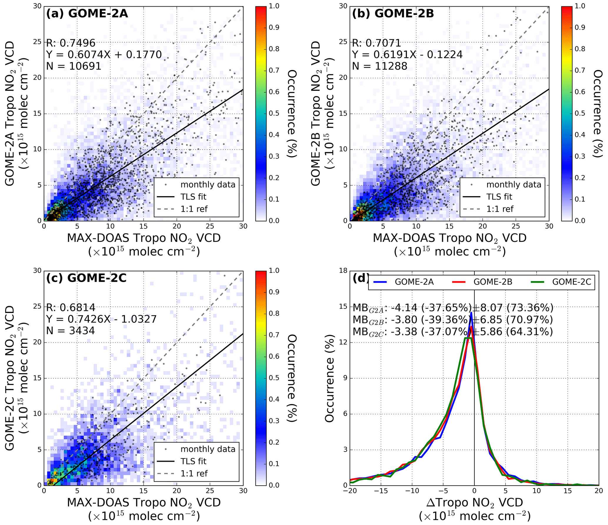
Figure 17 Comparison of daily and monthly tropospheric column NO₂ measured by the ground-based MAX-DOAS to (a) GOME-2A, (b) GOME-2B, and (c) GOME-2C. Histograms of the difference in tropospheric column NO₂ between GOME-2 and MAX-DOAS are shown in panel (d). Co-located daily and monthly averaged data are used in the comparison. Total least-squares regression is based on daily data.

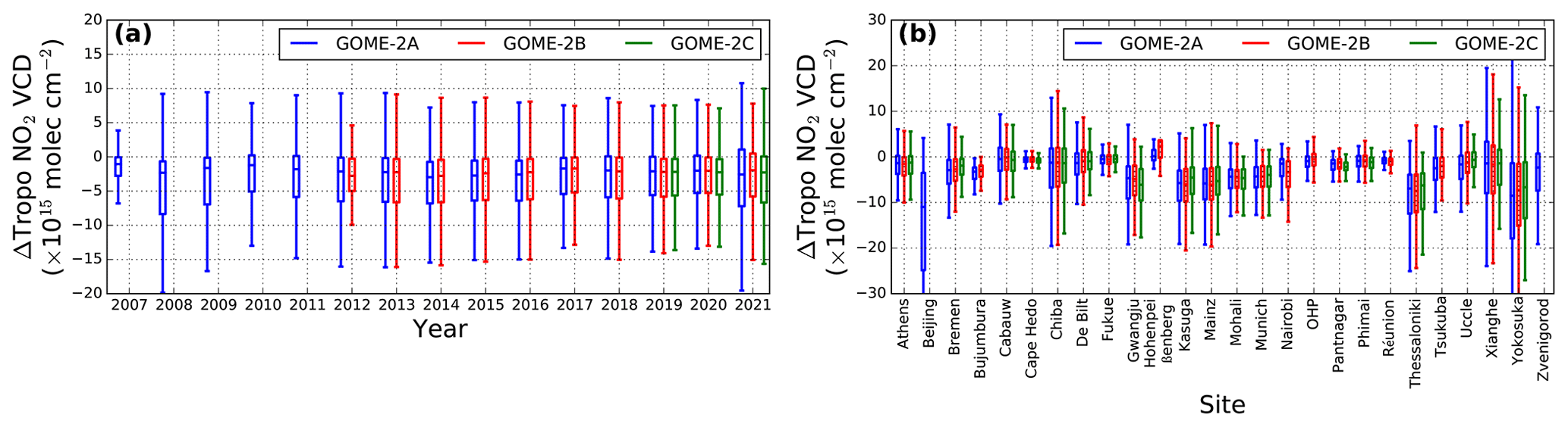
Figure 18 Comparison of tropospheric column NO₂ between ground-based MAX-DOAS and GOME-2 observations. Data are sorted by year in panel (a) and measurement site in panel (b).

Figure 18 shows box plots of the differences in tropospheric column NO₂ between the GOME-2 level-3 product and co-located MAX-DOAS measurements. Data are sorted by the measurement year (Fig. 18a) and measurement site (Fig. 18b). The mean differences between GOME-2 and MAX-DOAS observations are ∼ 3 × 10¹⁵ molec cm⁻² for most of the years, and this bias does not show significant temporal variation. Box plots for each measurement site show a significant negative bias for some polluted sites, i.e. Beijing (China), Thessaloniki (Greece), and Yokosuka (Japan). The reason for the negative bias has been explained above. The underestimation is significantly reduced over rural areas, e.g. Cape Hedo (Japan), Cabauw (Netherlands), and Phimai (Thailand). These results are in line with the level-2 data that GOME-2 in general underestimates tropospheric column NO₂ over polluted areas.

5.2.4 Total column water vapour

Daily GOME-2 level-3 total column water vapour is compared to the co-located sun-photometer observations. Figure 19 shows the density scatter plots for the comparison of the total column water vapour between GOME-2 and ground-based sun-photometer observations. Comparisons of GOME-2A, GOME-2B, and GOME-2C data are shown in Fig. 14a, b, and c, respectively. Histograms of the differences between GOME-2 and MAX-DOAS observations are shown in Fig. 19d. Similar plots for monthly comparison are shown in Fig. 20. GOME-2 monthly total column water vapour data are in general consistent with the daily data. GOME-2 daily observations are in good agreement with sun-photometer observations, with a Pearson correlation coefficient (R) of ∼ 0.92 for all three instruments. Monthly comparison shows a higher correlation coefficient (R) of ∼ 0.94. The slopes of least-squares regression lines of daily comparison for all three GOME-2 sensors are very close to 1, while a small offset of 1.2–1.6 kg m⁻³ is observed. Monthly comparison shows a similar characteristic, with the slope of regression close to 1 and an offset of 1.1–1.6 kg m⁻³. GOME-2 level-3 total column water vapour in general shows a positive bias of 1.0–1.7 kg m⁻³ (6 %–9 %). Considering that sun-photometer measurements in general underestimate total column water vapour by 6 % (Pérez-Ramírez et al., 2014), the positive bias of 1.0–1.7 kg m⁻³ is reasonable.

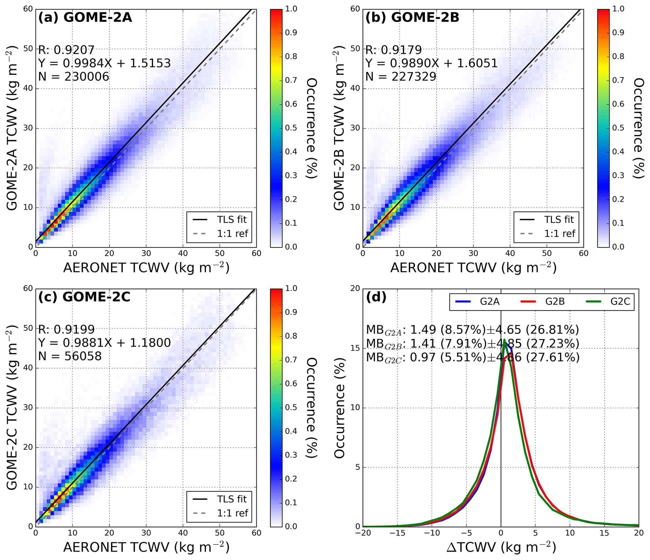
Figure 19 Comparison of daily total column water vapour measured by the sun photometer to (a) GOME-2A, (b) GOME-2B, and (c) GOME-2C. Histograms of the difference between GOME-2 and the sun-photometer are shown in panel (d). Co-located daily averaged data are used in the comparison.

Figure 20 Comparison of monthly total column water vapour measured by the sun photometer to (a) GOME-2A, (b) GOME-2B, and (c) GOME-2C. Histograms of the difference between GOME-2 and the sun photometer are shown in panel (d). Co-located monthly averaged data are used in the comparison.

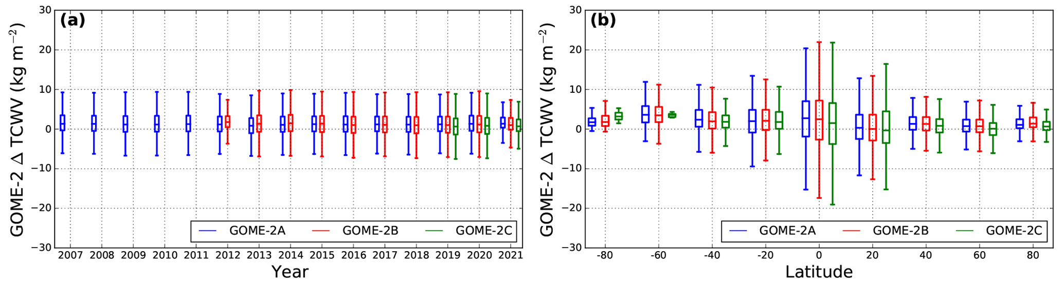
Figure 21 Comparison of TCWV between the sun-photometer and GOME-2 observations. Data are sorted by year in panel (a) and latitude in panel (b).

Figure 21 shows box plots of the statistic of the differences in total column water vapour between the GOME-2 level-3 product and co-located sun-photometer measurements. Data are sorted by the measurement year (Fig. 21a) and latitude band (Fig. 21b). The bias between GOME-2 and sun-photometer observations is consistently at the level of 1–2 kg m⁻³ throughout the entire measurement period. The latitude dependency analysis shows larger variations in the tropics, while the variations are much smaller at higher latitudes. The absolute differences for measurements over the polar regions are slightly higher. This is mainly due to multiple overpasses over the polar regions during summer months and the resulting temporal mismatch.

5.2.5 Total column BrO

Co-located daily and monthly GOME-2 level-3 total column BrO is compared to ZSL-DOAS observations at Harestua, Norway. Figure 22 shows the density scatter plots for the comparison of total column BrO between GOME-2 and ZSL-DOAS observations. Comparisons of GOME-2A, GOME-2B, and GOME-2C data are shown in Fig. 22a, b, and c, respectively. Monthly data are also shown as black dots. Histograms of the differences between GOME-2 and ZSL-DOAS observations are shown in Fig. 22d. We can see from the scatter plots that both GOME-2 and ZSL-DOAS BrO measurements are quite noisy: this is mainly due to the low absorption of BrO and thus the low signal-to-noise ratio. Both daily and monthly GOME-2 level-3 data show quite good agreement with the ZSL-DOAS observations, with a Pearson correlation coefficient (R) ranging from 0.64 to 0.74. In general, GOME-2 observations underestimate the BrO column by 7.0–10.2 × 10¹² molec cm⁻² (16 %–26 %). Please note that the comparison only covered one site in Norway and that the numbers might vary in different parts of the globe.

Figure 22 Comparison of daily and monthly total column BrO measured by the ground-based ZSL-DOAS at Harestua, Norway, to (a) GOME-2A, (b) GOME-2B, and (c) GOME-2C. Histograms of the difference in total column BrO between GOME-2 and MAX-DOAS observations are shown in panel (d). Co-located daily and monthly averaged data are used in the comparison. Total least-squares regression is based on monthly data.

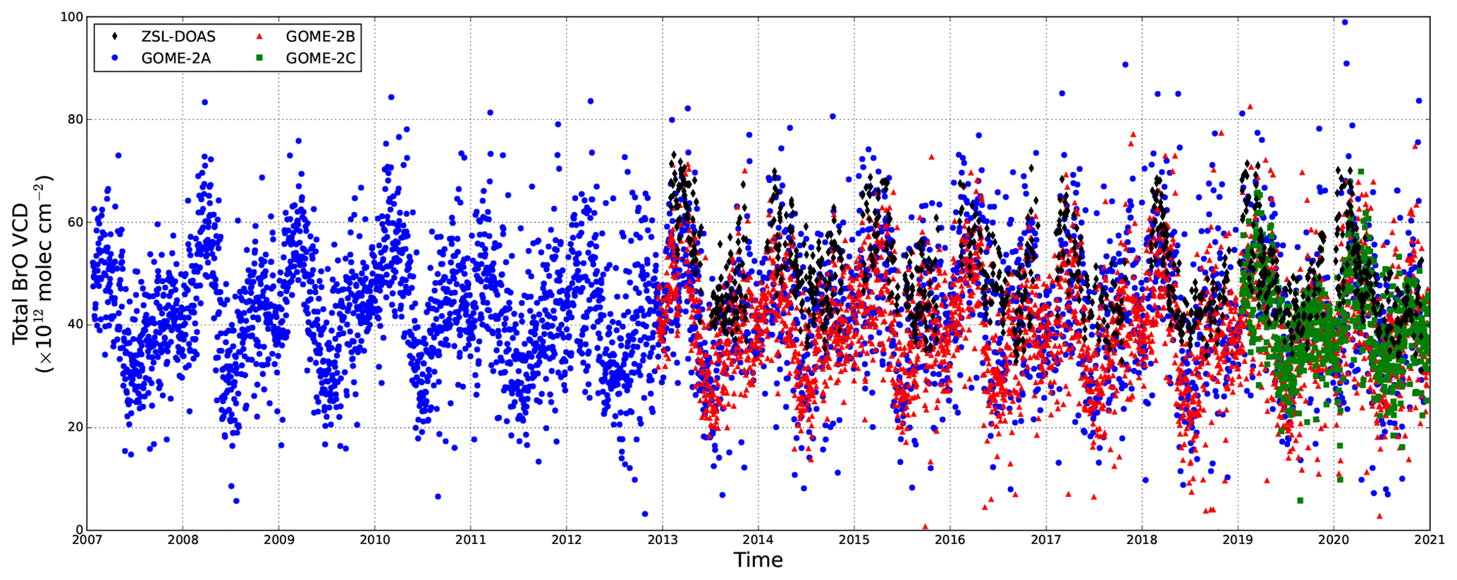
Figure 23 Time series of total column BrO measured by GOME-2A (blue), GOME-2B (green), GOME-2C (red), and ZSL-DOAS (black) at Harestua, Norway.

Figure 23 shows the time series of total column BrO measured at Harestua, Norway. Measurements from all three GOME-2 sensors show a similar temporal variation trend with a higher BrO level during winter/early spring and a lower one in summer, which agrees with the ZSL-DOAS observations. However, GOME-2 observations are about 5–10 × 10¹² molec cm⁻² lower than the ZSL-DOAS data. This underestimation has also been given in the level-2 validation report (Theys et al., 2015a). Considering that the ZSL-DOAS data have been empirically corrected for the offset caused by the instrumental effect, the agreement between GOME-2 and ZSL-DOAS is deemed very satisfactory.

5.2.6 Total column HCHO

Daily and monthly GOME-2 level-3 total column HCHO is compared to the co-located MAX-DOAS observations. Figure 24 shows the density scatter plots for the comparison of total column HCHO between GOME-2 and ground-based MAX-DOAS observations. Comparisons of GOME-2A, GOME-2B, and GOME-2C data are shown in Fig. 24a, b, and c, respectively. Monthly data are also shown as black dots. Histograms of the differences between GOME-2 and MAX-DOAS observations are shown in Fig. 24d. We can see from the scatter plots that both daily GOME-2 and MAX-DOAS HCHO measurements are quite noisy: this is mainly due to the low absorption of HCHO and thus the low signal-to-noise ratio. However, when we look at the monthly averages, the GOME-2 level-3 data in general agree with the ground-based MAX-DOAS observations. The Pearson correlation coefficient (R) between monthly GOME-2 and MAX-DOAS data ranges from 0.68 to 0.78. However, GOME-2 observations in general underestimate total column HCHO by 20 %–25 %. The slope of the total least-squares regression line for the comparisons of all three instruments varies from 0.74 to 0.81, with the offset ranging from −1.61 to −1.14 × 10¹⁵ molec cm⁻². GOME-2 level-3 total HCHO products on average show a small bias of −0.75 to 1.92 × 10¹⁵ molec cm⁻² (−7 %–17 %), with a standard deviation of 8.8 to 11.4 × 10¹⁵ molec cm⁻². The underestimation is partly related to the a priori profile used in GOME-2 retrieval and the difference in sensitivity between satellite and ground-based observations. The underestimation of the level-3 product is in line with the level-2 product. Previous studies show that the negative bias is significantly improved when the MAX-DOAS profiles are used for satellite column retrieval (De Smedt et al., 2015a, b). As the daily level-3 HCHO data are a bit noisy, it would be useful to further average the data spatially to reduce noise when looking into day-to-day variability or to use the temporally averaged product, i.e. the monthly product.

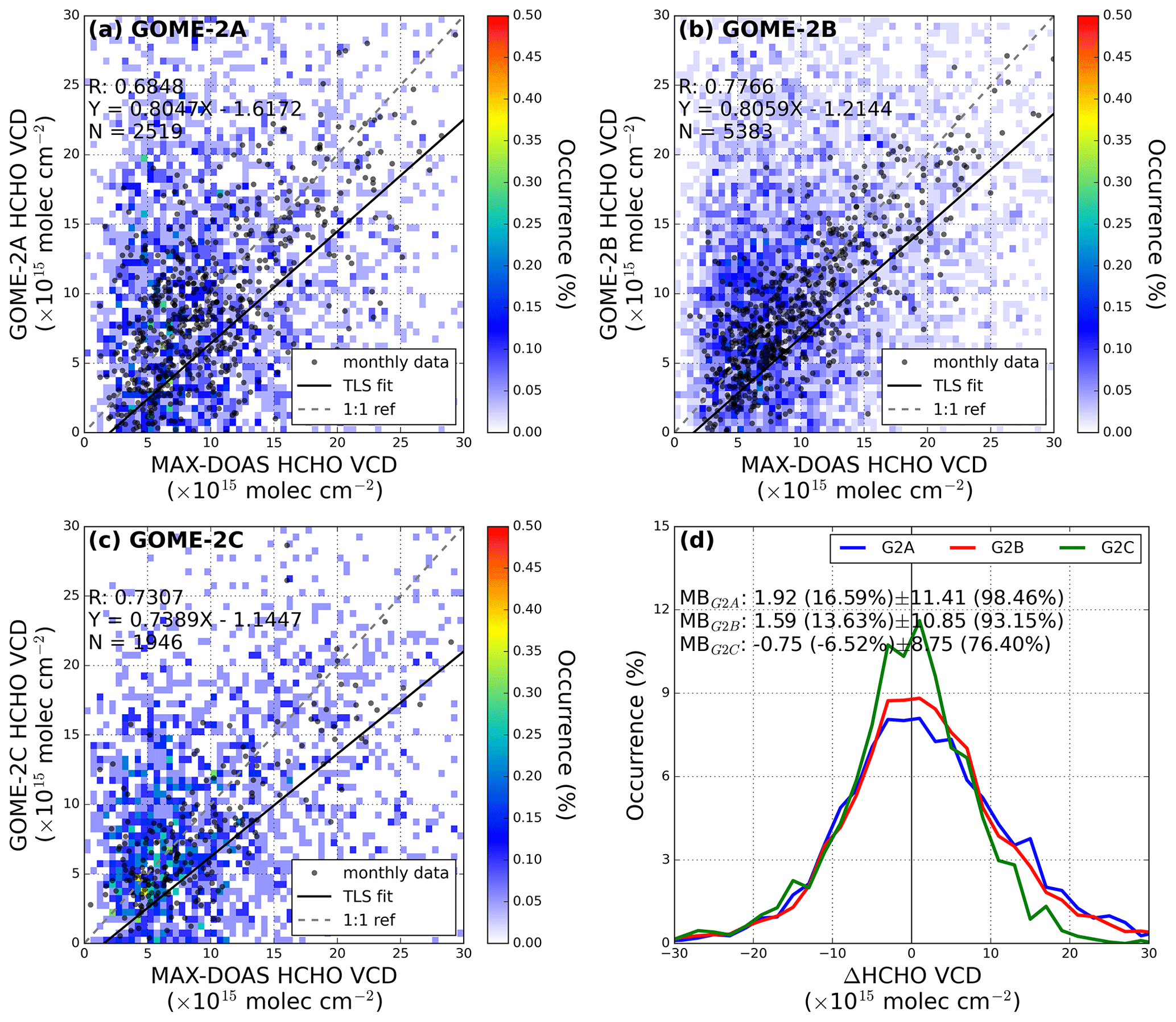
Figure 24 Comparison of daily and monthly total column HCHO measured by the ground-based MAX-DOAS to (a) GOME-2A, (b) GOME-2B, and (c) GOME-2C. Histograms of the difference in total column HCHO between GOME-2 and MAX-DOAS are shown in panel (d). Co-located daily and monthly averaged data are used in the comparison. Total least-squares regression is based on monthly data.

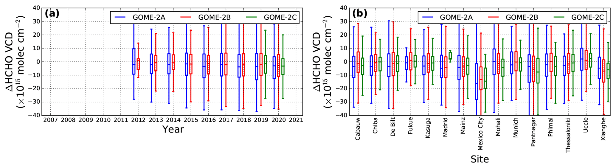
Figure 25 Comparison of total column HCHO between ground-based MAX-DOAS and GOME-2 observations. Data are sorted by year in panel (a) and measurement site in panel (b).

Figure 25 shows box plots of the statistic of the differences in total column HCHO between the GOME-2 level-3 product and co-located MAX-DOAS measurements. Data are sorted by the measurement year (Fig. 25a) and measurement site (Fig. 25b). The mean differences between GOME-2 and MAX-DOAS observations are 1–2 × 10¹⁵ molec cm⁻² for most of the years and do not show significant temporal variation. Box plots for each measurement site show that GOME-2 significantly underestimated the HCHO column over polluted areas, i.e. Mexico City (Mexico) and Xianghe (China). The underestimation is related to the difference in sensitivity, and this effect has been reported in previous level-2 validation studies for GOME-2 (De Smedt et al., 2015b; Pinardi et al., 2020b) as well as for other satellites (Chan et al., 2020b; De Smedt et al., 2021).

5.2.7 Total column SO₂

The validation of volcanic SO₂ is very difficult due to the differences in volcanic plume injection height for each eruption. Therefore, it is often done in a case study base, i.e. in previous validation reports (Theys et al., 2015b). In this study, we focus on the long-term statistic and stability and therefore look mainly into areas with significant SO₂ sources. Co-located daily and monthly GOME-2 level-3 total column SO₂ is compared to Pandora observations at Mexico City. Figure 26 shows the scatter plots for the comparison of total column SO₂ between GOME-2 and Pandora observations. Comparisons of GOME-2A, GOME-2B, and GOME-2C data are shown in Fig. 26a, b, and c, respectively. Monthly data are also shown as black dots. Histograms of the differences between GOME-2 and Pandora observations are shown in Fig. 26d. Due to the low absorption and abundance of SO₂, both GOME-2 and Pandora measurements are quite noisy. The histogram shows that GOME-2 underestimated total column SO₂ by 0.25 to 0.48 DU (47 %–64 %). This underestimation is likely related to the a priori profiles used in AMF calculations. The product assumes an SO₂ plume at 6 km. If an a priori SO₂ located in the lower troposphere is used in the AMF calculations, it would increase the retrieved SO₂ columns and reduce the underestimation. Please be aware that this is just a comparison over one site in Mexico and that the numbers might vary over different parts of the globe, especially due to the low concentration of SO₂ in general.

Figure 26 Comparison of daily and monthly total column SO₂ measured by the Pandora instrument in Mexico City to (a) GOME-2A, (b) GOME-2B, and (c) GOME-2C. Histograms of the difference in total column SO₂ between GOME-2 and Pandora observations are shown in panel (d). Co-located daily and monthly averaged data are used in the comparison. Total least-squares regression is based on daily data.

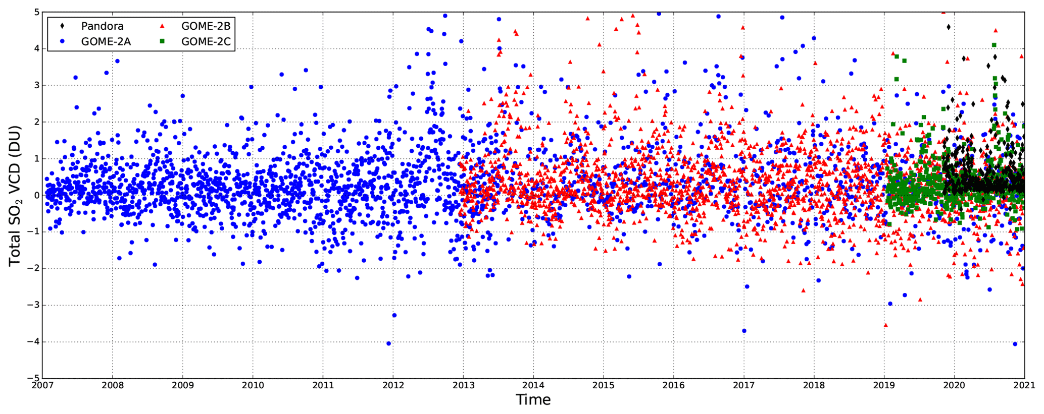
Figure 27 Time series of total column SO₂ measured by GOME-2A (blue), GOME-2B (green), GOME-2C (red), and Pandora (black) at Mexico City.

Figure 27 shows the time series of total column SO₂ measured at Mexico City. All three GOME-2 sensors show similar SO₂ columns. The overall averages are very close to 0 and do not show any significant trend. Due to the low abundance of SO₂ and a low signal-to-noise ratio, there are a considerable number of negative values. On the other hand, due to the better signal-to-noise ratio, only a very few negative values were measured by Pandora. Considering the measurement noise of GOME-2, the agreement between the GOME-2 and Pandora data sets is reasonable.

6 Data availability

The GOME-2 level-3 products described in this paper are available to the public via EUMETSAT’s Satellite Application Facility on Atmospheric Composition Monitoring (https://acsaf.org, last access: 15 March 2023). DOIs: daily products https://doi.org/10.15770/EUM_SAF_AC_0048 (AC SAF, 2023a); monthly products https://doi.org/10.15770/EUM_SAF_AC_0049 (AC SAF, 2023b).

7 Summary

We presented the new GOME-2 daily and monthly level-3 products, which include total column O₃, total and tropospheric column NO₂, total column water vapour, total column BrO, total column HCHO, and total column SO₂. Compared to satellite observations from OMI and TROPOMI, which measure at noon or in the early afternoon, GOME-2 measurements in the morning provide addition information on the temporal/diurnal variation of these atmospheric trace gases. This additional information would be very useful for the studies of temporal/diurnal variations and photochemistry in the atmosphere. Details of the algorithm for level-2 to level-3 processing as well as the selection of an appropriate spatial resolution for the level-3 products are shown. Verification and validation of each GOME-2 level-3 product are achieved by investigating the consistency among the three GOME-2 sensors and comparison to ground-based reference measurements.

The overlapping area-weighting method is used for level-2 to level-3 processing. The spatial resolution of the GOME-2 level-3 products is selected based on the sensitivity study. The consistency among the three GOME-2 sensors is investigated through time series of global averages, zonal averages, and biases. Finally, the accuracy of the level-3 products is validated through the comparison to ground-based observations.

For the selection of an appropriate spatial resolution of the GOME-2 level-3 data, we have re-sampled GOME-2 level-2 data onto various spatial resolutions, i.e. 0.1^∘ × 0.1^∘, 0.25^∘ × 0.25^∘, and 0.5^∘ × 0.5^∘, and compared them to the original level-2 data. All the data sets show very similar spatial structures, and the absolute values are consistent with the level-2 products. As expected, level-3 data sampled at a higher spatial resolution (i.e. 0.1^∘ × 0.1^∘) better preserved the original GOME-2 instrument footprint. However, a lower resolution of 0.25^∘ × 0.25^∘ also preserves the spatial pattern of quickly varying tropospheric species, i.e. NO₂, reasonably well, while a rather strong smoothing/averaging effect is observed from data gridded with a lower spatial resolution (i.e. 0.5^∘ × 0.5^∘). Therefore, we concluded that the spatial resolution of 0.25^∘ × 0.25^∘ is sufficient and appropriate for GOME-2 level-3 products.

The consistency of the level-3 product among the three GOME-2 sensors is investigated. Global-average time series plots show that total column ozone and water vapour products from all the GOME-2 sensors are consistent, with only a small bias of up to 3 DU (<1 %) for ozone and 0.9 kg m⁻² (<5 %) for water vapour. For total and tropospheric column NO₂ products, GOME-2A and GOME-2B measurements are consistent with each other, while GOME-2C data show significant discrepancy compared to the other two sensors. This is mainly due to the differences in processor versions (GDP 4.8 for GOME-2A and GOME-2B and GDP 4.9 for GOME-2C) and the spectral-fitting band of NO₂. BrO observations from GOME-2B in general show a negative bias of 1.0–1.5 × 10¹² molec cm⁻² compared to GOME-2A and GOME-2C. GOME-2A HCHO columns are 1.5–1.9 × 10¹⁵ molec cm⁻² lower than GOME-2B and GOME-2C measurements. This is due to the underestimation over the Amazon, Southeast Asia, and Australia. Total column SO₂ observations from GOME-2C are on average 0.5 DU lower than GOME-2A and GOME-2B, resulting in a slightly negative global average. A slightly higher global average of SO₂ measured by GOME-2A and GOME-2B is related to the high values taken under extreme viewing geometry, i.e. a high solar zenith angle. Please be reminded that BrO and SO₂ products are only validated against measurements at specific locations, which might need to be further validated depending on the user applications.

For comparison of co-located GOME-2 level-3 data to ground-based observations, we found in general good agreement, and the results are consistent with previous level-2 validation studies. We summarize the statistical result in Table 3.

From the results above, we conclude that the daily and monthly GOME-2 level-3 products of total column O₃, total and tropospheric column NO₂, total column water vapour, total column BrO, total column HCHO, and total column SO₂ for GOME-2A, GOME-2B, and GOME-2C are consistent and fulfil the product requirements.