Ocean cross-validated observations from R/Vs L'Atalante, Maria S. Merian, and Meteor and related platforms as part of the EUREC⁴A-OA/ATOMIC campaign

The northwestern Tropical Atlantic Ocean is a turbulent region, filled with mesoscale eddies and regional currents. In this intense dynamical context, several water masses with thermohaline characteristics of different origins are advected, mixed, and stirred at the surface and at depth. The EUREC⁴A-OA/ATOMIC experiment that took place in January and February 2020 was dedicated to assessing the processes at play in this region, especially the interaction between the ocean and the atmosphere. For that reason, four oceanographic vessels and different autonomous platforms measured properties near the air–sea interface and acquired thousands of upper-ocean (up to 400–2000 m depth) profiles. However, each device had its own observing capability, varying from deep measurements acquired during vessel stations to shipboard underway near-surface observations and measurements from autonomous and uncrewed systems (such as Saildrones). These observations were undertaken with a specific sampling strategy guided by near-real-time satellite maps and adapted every half day, based on the process that was investigated. These processes were characterized by different spatiotemporal scales, from mesoscale eddies, with diameters exceeding 100 km, to submesoscale filaments of 1 km width. This article describes the datasets gathered from the different devices and how the data were calibrated and validated. In order to ensure an overall consistency, the platforms' datasets are cross-validated using a hierarchy of instruments defined by their own specificity and calibration procedures. This has enabled the quantification of the uncertainty in the measured parameters when different datasets are used together, e.g., https://doi.org/10.17882/92071 (L'Hégaret et al., 2020a).

1 Introduction

The international EUREC⁴A-ATOMIC initiative (http://eurec4a-oa.eu/, last access: 17 April 2023) aimed to better understand the link between atmospheric shallow convection, cloud formation, and the general circulation of the atmosphere (Stevens et al., 2021). The EUREC⁴A-OA experiment was embedded in EUREC⁴A-ATOMIC and took place in January and February 2020 in the northwestern Tropical Atlantic Ocean. EUREC⁴A-OA focused on the impact of mesoscale and submesoscale regional ocean dynamics on processes at the air–sea interface. The targeted ocean sampling for EUREC⁴A-OA was done with four research vessels (R/Vs), namely Germany's Maria S. Merian (Karstensen et al., 2020) and Meteor (Mohr et al., 2020), France's L'Atalante (Speich et al., 2021b), and the USA's Ronald H. Brown (Quinn et al., 2021). In addition, various autonomous platforms, underwater electric gliders, surface drifters, Argo profiling floats, Saildrones, and prototype drifting buoys, OCARINA and PICCOLO (Bourras et al., 2014), were operated in coordination with the ships.

The EUREC⁴A-ATOMIC experiment took place in a rich dynamical context, where several water masses of diverse origins are advected (see Fig. 1), stirred, and mixed but also preserve, however, large horizontal and vertical contrasts. Figure 1 in Fratantoni and Glickson (2002) summarizes the main upper-ocean features. The research vessels and platforms deployed during the experiment focused on two subregions, namely one east of Barbados characterized by a rather stable wind regime of easterlies (trade wind alley) and the other to the south and bounded by the South American continent, which is a region that hosts intense and long-lived northwestward-drifting mesoscale eddies spawned by North Brazil Current (NBC) retroflection (eddy boulevard). Also, along the shelf break, the Amazon River plume flows northward and actively interacts with the North Brazil Current and its mesoscale eddies, called the NBC rings (Fratantoni and Glickson, 2002; Fratantoni and Richardson, 2006). The evolution, characteristics, and inter- to intra-annual variability, of NBC rings are important elements of the global ocean circulation. As the North Brazil Current sheds eddies that move northward along the South American continental slope, they provide an essential part of the interhemispheric transport of mass, heat, salt, and many different biogeochemical ocean properties and thus have a key role in the Atlantic Meridional Overturning Circulation (AMOC; Johns et al., 2003). In this study, we will use the devices deployed by R/V Meteor (mainly focused on the trade wind alley) and by R/Vs L'Atalante and Maria S. Merian (sampled the eddy boulevard). We will focus on the oceanic measurements (temperature, salinity, oxygen, and velocity) and leave aside the atmospheric and meteorological ones, some of which are already discussed in companion papers in this journal's special issue that is dedicated to EUREC⁴A (Bailey et al., 2023; Bosser et al., 2021; Stephan et al., 2021), and others will be submitted soon.

Figure 1 Bathymetric map of the northern Tropical Atlantic Ocean, with the EUREC⁴A-OA/ATOMIC regions of interest framed in orange for the trade wind alley and in red for the eddy boulevard. The main surface currents of these two regions are schematically represented in black. NBC stands for the North Brazil Current.

For observational studies of mesoscale/submesoscale features, some means of adaptive sampling is required. The EUREC⁴A-OA sampling was guided by analysis of near-real-time satellite maps of sea surface temperature, sea surface salinity, altimetry (absolute dynamic height and related geostrophic velocities) and ocean color (Speich et al., 2021b). Guided by the satellite information, the surveys were then done by various observational platforms in order to sample specific features, such as mesoscale eddies and fronts, freshwater pools, and filaments. To address the anticipated spatiotemporal sampling, the various platforms with different resolutions, autonomy, sensor payloads (Liblik et al., 2016), and periods required to acquire a profile were used in a concerted effort (Fig. 2). The sampling strategy was designed such that the phenomena would be measured with sufficient temporal and spatial resolution, while also paying attention to the synchronicity of observations in the ocean and atmosphere.

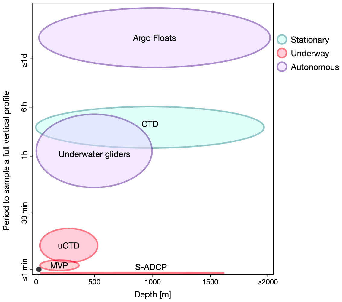
Figure 2 Schematic representation of the devices deployed during the EUREC⁴A-OA experiment, characterized by their frequency of acquisition for a full vertical profile and depth reached, considering the time of deployment. The green color indicates observations undertaken with the docked ship. The red color designates the devices acquiring data underway, whereas the purple color represents autonomous platforms. The dot in the lower left corner represents the surface measurements made by the ships' thermosalinograph (TSG), Saildrones, and surface drifters.

In order to ensure interoperable data for a parameter measured with various sensors, a comparative quality analysis was also performed, known as secondary quality control (QC). Secondary QC aims to create a coherent dataset out of various data streams.

Gouretski and Jancke (2000) were among the first to present secondary QC on oceanographic data through the use of a crossover analysis in deep waters. This enabled them to conduct a rigorous QC assessment by comparing data from different sources and determining systematic errors such as standard seawater batch offsets. As for other similar studies (e.g., Tanhua et al., 2010), a basic assumption is that deep-water (typically >2000 m) properties are close to invariant. The need for QC methods in the upper layer received much attention through the global operations of profiling floats that typically are not recovered and hence receive direct sensor QC only before deployment (e.g., in the lab and in reference to a standard or to reference material). As introduced by, for example, Wong et al. (2003), by comparing with all nearby profile data and considering distance in space and time as a measure for impact, the offset and drift behaviors of specific float measurements can be reconstructed.

The goal is to perform a quality assessment of a dataset, which in turn is composed of individual datasets from different observation platforms and sensors. For this purpose, here we introduce an assessment scheme of the individual datasets based on their traceability to reference data (traceability level). In the most optimal case, the reference material (RM) is a de facto standard (Otosaka et al., 2020), such as standard seawater for salinity, oxygen titration for dissolved oxygen, or triple-point cells for temperature. As an example, for salinity the RM is standard seawater (SSW), giving a hierarchy as follows, where SSW is assigned traceability level 0 and used to reference a salinometer (Bacon et al., 2007) (traceability level 1). The salinometer readings for bottle samples are used as a statistical basis for the ship's CTD (conductivity, temperature, and depth) salinity correction (traceability level 2). The corrected ship CTD salinity is then further used to correct the thermosalinograph (TSG; traceability level 3). Bottle samples were also collected for the TSG and used via the salinometer as a statistical basis for the ship's CTD salinity correction (traceability level 2). The TSG is used to correct the Saildrones data (traceability level 4 or level 3, depending on the TSG calibration). Similar hierarchies can be built for all sensors.

Part of the quality assurance of the combined dataset is determining accuracy and precision and also considering in this process the expected stability of the sensors given by the manufacturer. The CTD rosette is key in the calibration process with respect to the secondary QC. From the water samples collected with the rosette sampler, numerous variables (in addition to conductivity, temperature, and pressure) are accessible throughout the water column, which is used for sensor calibration, laboratory analysis (e.g., oxygen titration), and to analyze biogeochemical parameters. However, its deployment requires the ship to remain on station for a few hours (depending on the attained depth) to perform the vertical profiles. The underway CTD (uCTD) and Moving Vessel Profiler (MVP) casts can be carried out underway, but they cannot dive deeper than about 450 m for the uCTD and about 200 m for the MVP model we employed (MVP30–300; Branellec et al., 2020; Karstensen et al., 2020; Speich et al., 2021b). Also, their sensors are more subject to bias than the CTD (Ullman and Hebert, 2014). Other devices, such as underwater gliders, drifters, and Argo floats, are autonomous, but the data calibration is limited to certain times (deployment and recovery is as shown in Fig. 2) or by comparing sensor readings from nearby (time and space) data that have passed a QC. All the underway and autonomous devices rely on the proximity in space and time of CTD casts to validate and calibrate their measurements.

In the following section, we present the calibration strategy adopted in this study, in addition to the hierarchy of traceability between the sensors of each device. In Sect. 3, we present the ship observations, providing information on when and where they were deployed and how they were calibrated and validated. There, we focus on the CTD and how they are used to estimate the uncertainty in platforms with a lower level of traceability. Section 4 is constructed similarly but focuses on autonomous devices. In Sect. 5, we provide an example of data concatenation of different platforms. Finally, we describe the final dataset and the variables we provide for use to the scientific community.

2 Calibration strategy

The EUREC⁴A-OA experiment relied on numerous devices to measure the physical and chemical properties of the water column from the three European ships and the various autonomous platforms deployed from the ships. We also include here the five USA Saildrones funded under the NOAA and NASA ATOMIC project (Quinn et al., 2021; Gentemann et al., 2020). Their deployments were conducted by scientific staff originating from two institutions, namely GEOMAR (Kiel, Germany) and IFREMER (Brest, France). They have specific practices, sometimes leading to different procedures of deployment, data acquisition, and calibration, while still complying with international standards (Sloyan et al., 2019). The various calibration practices are either linked to similar devices from different manufacturers or to various procedures in laboratories before and after the cruise. All of the devices deployed during EUREC⁴A-OA are commonly used in oceanographic cruises, and the sources of errors and calibration procedures have been extensively documented and studied. In the next section, we briefly summarize them for each device.

At the top level of our hierarchy stands the most traceable sensors used to read water samples issued from the CTD bottles during every vertical profile or from the TSG circuit.

The CTD measurements are at the second level of the hierarchy, as its sensors went through careful pre-cruise and post-cruise calibration at the manufacturer's facility. Moreover, the sensor measurements are carefully validated and calibrated with samples collected and analyzed from the rosette bottle water samples. CTD measurements serve as references for the calibration of all other observing platforms. Some TSG underway measurements also stand at traceability level 2 when calibrated with bottle samples.

Next in the ranking (traceability level 3) come those devices whose measurements are calibrated with the CTD, as they sample the same water (devices located on the same ship from which the CTD was deployed and measuring the same water as the CTD). These are the TSGs, when not directly calibrated with bottle samples, and the uCTD sensors, when the probes were purposely mounted for calibration on the CTD rosette. The main sources of error here come from the method of deployment of the devices and the sampling rate of the sensors.

Sensor data that are only calibrated via reference data close in space and time to the CTD profiles are labeled with traceability level 4. The cross-calibration is then achieved by comparing the vertical profiles on temperature/salinity (T/S) and depth/density diagrams. Most of the underway profiling devices fall into this category, i.e., uCTD, MVP, and underwater gliders. As these measurements are not synchronous and not co-located with CTD profiles, an additional source of uncertainty arises from the spatiotemporal ocean variability.

At the bottom of the hierarchy of traceability to a standard or an RM are the devices that cannot be compared directly either because their sensors are specific, measuring quantities that are not directly comparable with the CTD, or can only be calibrated by the manufacturers.

3 Ship observations

3.1 CTD rosette

On R/Vs Maria S. Merian, Meteor, and L'Atalante a Sea-Bird SBE911+ CTD system was used for high-quality vertical profiling of the water column. Hereafter, we will briefly describe the calibrations and validations for each sensor. Other sensors were mounted to the CTD device (e.g., fluorescence, turbidity, and particles) but are not considered here. Similar operational practices were carried out on all ships for CTD profiling. First, the CTD system was lowered to shallow depth (5 m) until the pump started. Then the CTD was brought back to the surface and subsequently lowered at approximately 0.5 m s⁻¹ in the first 100 m and 1 m s⁻¹ for the deeper water column. The target depth varied but in most cases reached just above the seafloor. Water samples were collected with Niskin bottles mounted to the CTD rosettes. The samples were used for sensor calibration and for further analysis. The procedure for closing the bottles differed between the ships. On R/V L'Atalante, the CTD was stopped for a few seconds for sampling, while on R/V Maria S. Merian, the samples were taken without stopping the CTD package. In total the number of profiles acquired were 64, 86, and 266 for R/Vs L'Atalante, Maria S. Merian, and Meteor, respectively (Fig. 3).

The CTD rosettes on R/Vs Maria S. Merian and L'Atalante were also equipped with two lowered acoustic Doppler current profilers (L-ADCPs), in a system composed of one instrument looking upward and the other one looking downward, to record ocean current profiles.

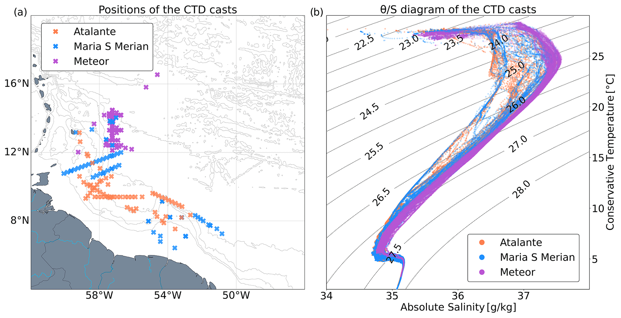
Figure 3 (a) Map of the CTD cast positions for R/Vs L'Atalante, Maria S. Merian, and Meteor. (b) θ/S (temperature/salinity) diagram of the CTD profiles for each ship superimposed on the isopycnals.

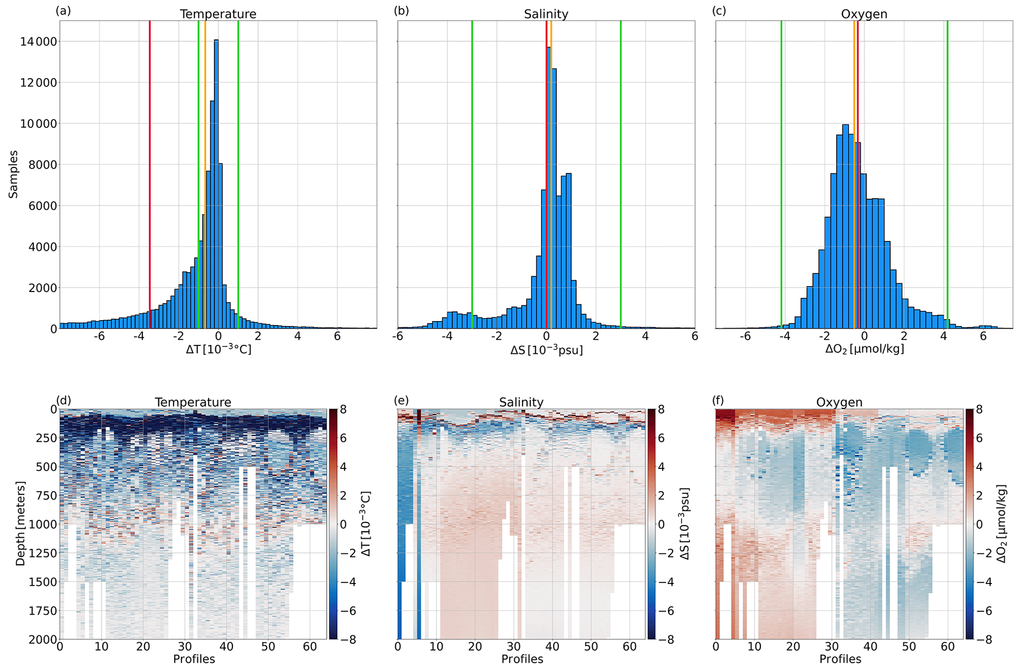
Figure 4 Panels (a), (b), and (c) show histograms displaying the differences, respectively, in temperature, salinity, and oxygen between the IFREMER and GEOMAR calibrations applied to R/V L'Atalante CTD profiles. Green lines indicate the accuracy claimed by the manufacturer, and red and orange lines show the mean and median differences. Panels (d), (e), and (f) display these differences vertically for each CTD profile.

3.1.1 Pressure, temperature, conductivity, and salinity quality assurance

Based on the manufacturer (Sea-Bird) specifications, the SBE9+ probe measures pressure with an initial accuracy of $\pm \mathrm{1.5}\times {\mathrm{10}}^{-\mathrm{2}}$ % and a resolution of $\pm \mathrm{1}\times {\mathrm{10}}^{-\mathrm{3}}$ % of the full scale of the respective CTD (6800 m for R/Vs Maria S. Merian and Meteor).

For R/V L'Atalante, the pressure sensors are calibrated before and after the cruise at the IFREMER Laboratory of Metrology. The calibration is performed at a constant temperature of 20 ^∘C, with increasing and decreasing pressure levels and with an uncertainty of 0.6 dbar at 2000 dbar. The bias, measured during the calibration, is then corrected by a polynomial of degree 4, which is associated with an uncertainty of ±0.12 dbar. A good stability of the sensor was observed, with an overall uncertainty of ±0.72 dbar. In addition, a validation was made using reversing pressure meter sensors (SIS RPM 6000 X) at the bottom of the profiles and by comparing them with the CTD sensor to assess any drift. No drift was observed during the cruise; so after the laboratory calibration and in-cruise validation, we assign the CTD pressure sensor level 2 traceability and an uncertainty of the order of the initial sensor accuracy of $\pm \mathrm{1.5}\times {\mathrm{10}}^{-\mathrm{2}}$ %. For the pressure sensors of R/Vs Maria S. Merian and Meteor, no dedicated lab calibration is carried out.

For all ships, the pressure sensor offset on deck before and after each profile was corrected in the processing as an offset, which was typically the mean of all values for each probe.

For each CTD, two SBE3+ temperature sensors from Sea-Bird were mounted on the SBE911 probe, and the most stable sensor was used for the final calibration. The accuracy and resolution provided by the manufacturer are of $\pm \mathrm{1}\times {\mathrm{10}}^{-\mathrm{3}}$ and $\pm \mathrm{2}\times {\mathrm{10}}^{-\mathrm{4}}$ ^∘C.

For R/V L'Atalante, the temperature readings were calibrated at the IFREMER Laboratory of Metrology before and after the cruise in reference to a Rosemount-type platinum resistance, periodically checked and certified, in a bath with strictly controlled temperature. The measurements were corrected by applying a polynomial of degree 3. The maximal error is lower than the sensor accuracy provided by the manufacturer. In addition, the temperature sensor stability was monitored in comparison with two reversing thermometers (SIS RTM 4002 X), where one was closed at the deepest depth of the profile and the other during the descent. No drift was observed during the cruise. For R/Vs Maria S. Merian and Meteor, the sensors were calibrated before the cruise at an authorized lab.

For the temperature sensors from the CTD, we thus assume an uncertainty of $\mathrm{1}\times {\mathrm{10}}^{-\mathrm{3}}$ ^∘C, corresponding to the manufacturer accuracy, and we assign them level 2 traceability in our hierarchy.

Conductivity is measured with two Sea-Bird SBE4 sensors, and as for temperature, the most stable sensor is used for the final calibration. In general, the procedures followed the GO-SHIP recommendations in Hood et al. (2010), but details are provided below. The accuracy of the SBE4, as provided by the manufacturer, is $\pm \mathrm{3}\times {\mathrm{10}}^{-\mathrm{3}}$ mS cm⁻¹, with a nominal stability of $\mathrm{3}\times {\mathrm{10}}^{-\mathrm{4}}$ per month and a resolution of $\pm \mathrm{4}\times {\mathrm{10}}^{-\mathrm{5}}$ mS cm⁻¹ at 24 Hz sampling.

For sensors used on R/Vs, a lab calibration was done before the cruise by a manufacturer-authorized (Sea-Bird) laboratory. During the cruises, water samples were collected from Niskin bottles to perform a CTD conductivity calibration. The salinity of the water samples was analyzed on R/V Maria S. Merian using an OPTIMARE salinometer and on R/V L'Atalante using a Portasal salinometer. The salinometers were in turn calibrated against a reference material, standard seawater. On R/V Maria S. Merian, a secondary reference was also used (labeled as substandard), which is a large volume of water with unknown but constant salinity. At regular intervals, the substandard was measured with the salinometer and tracked for stability as an indicator of potential drift of the salinometer without the need to use large volumes of standard seawater. One other slight difference in the procedures was the treatment of the water samples before analysis with the salinometer. In addition to adjusting the samples to the laboratory temperature (R/Vs Maria S. Merian and L'Atalante), the samples were degassed on R/V Maria S. Merian. On earlier cruises, it was found that the OPTIMARE salinometer is more sensitive to gas bubbles. For the purpose of degassing, the bottles were heated in a water bath to 5–10 ^∘C above laboratory temperature and then brought back to laboratory temperature. The released gas was extracted. Only then were the samples analyzed. More information on the CTDs and salinometers can be found in the cruise reports (Karstensen et al., 2020; Branellec et al., 2020). The salinity data from bottle samples of R/Vs Maria S. Merian and L'Atalante is considered level 1 traceability.

The processing of CTD conductivity was done by first applying basic processing steps from the SBE (Sea-Bird Electronics) processing routines (SeasoftV2) and including a loop edit (0.2 ms). The prepared raw data were then calibrated using the bottle sample analysis. Slightly different approaches were taken for R/Vs Maria S. Merian and L'Atalante.

R/V Meteor did not have a salinometer on board. Samples were collected and stored on board for later analysis on shore. However, the number of samples available was too small to perform a meaningful statistical analysis. At two occasions, CTD profiles from R/Vs Maria S. Merian and Meteor were performed close in space (1500 and 50 m apart) and covered the full water column. They are used here for the purpose of R/V Meteor CTD sensor calibration and validation. A −4 db offset was found between the profiles. As a consequence, we applied an equivalent correction to R/V Meteor measurements. This led us to consider R/V Meteor CTD data at level 3 in traceability.

For R/V Maria S. Merian, the processing was as follows. After allocating a downcast profile segment to the upcast bottle sample stop via a vertical gradient criterion, the conductivity difference between the bottle sample analysis and CTD sensor recording was calculated. The differences were sorted by magnitude, and the first 33 % of all values were removed to eliminate outliers. Based on the remaining 66 % of all values, correction equations were derived using the pressure, conductivity, time, and sample number. Care was taken to not use higher-order equations, as spurious interpolation may appear for weakly constrained segments of the multiparameter fit space. The uncertainty in R/V Maria S. Merian sensors is estimated to be $\mathrm{2}\times {\mathrm{10}}^{-\mathrm{3}}$ psu, and the data are assigned level 2 traceability. A similar procedure was used for the oxygen sensor calibration based on the results from the Winkler titration.

For R/V L'Atalante, a set of three corrections was applied to remove large differences between the conductivity values of the sensor and water sample. First, a correction as a function of time was implemented to take into account a potential slow drift of the conductivity sensor. Second, a correction relative to the conductivity was applied. At each iteration of this correction, the samples showing $\mathrm{\Delta }C>\mathrm{2.8}\times \mathit{\sigma }$, with ΔC being the difference between the sensor and the water sample conductivity and σ the standard deviation of all the samples considered at each iteration, were removed. Third, a correction as a function of pressure was applied to the conductivity or salinity. After the calibration of all casts, the standard deviation between the sensor data and the chemical data was $\mathrm{2.3}\times {\mathrm{10}}^{-\mathrm{3}}$ mS cm⁻¹ for conductivity and $\mathrm{2.3}\times {\mathrm{10}}^{-\mathrm{3}}$ psu for salinity, which are both below the accuracies provided by Sea-Bird. The uncertainty in the sensors of R/V L'Atalante is thus of $\mathrm{3}\times {\mathrm{10}}^{-\mathrm{3}}$ psu, and they are considered level 2 traceability.

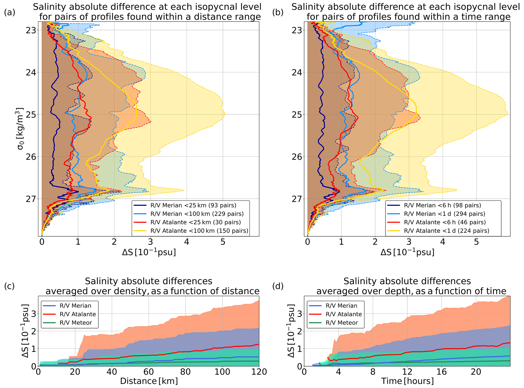
Figure 5 (a) Absolute salinity difference between CTD pairs of profiles calculated on isopycnal levels for each R/V, averaged by distance. The dark blue and red curves are the average differences for profiles that are separated by less than 25 km for R/Vs Maria S. Merian and L'Atalante, respectively, while the blue and orange curves are for profiles found within 100 km. The shaded areas represented the standard deviation at each isopycnal level. (b) Same as panel (a) but with profiles averaged by time. The dark blue and red curves are for profiles separated by less than 6 h, while the blue and orange curves are found within the same day, again for R/Vs Maria S. Merian and L'Atalante, respectively. (c) Absolute salinity differences averaged vertically over the isopycnal levels as a function of distance for R/Vs Maria S. Merian (blue), L'Atalante (red), and Meteor (green). (d) Same as panel (c) but as a function of time instead of distance.

Figure 6 (a) Absolute temperature differences between CTD pairs of profiles on isopycnal levels, averaged and vertically distributed in time and distance. Each CTD pair is only composed of profiles from R/Vs L'Atalante or Maria S. Merian. (b) Same as panel (a) but for CTD pairs composed of one profile from R/V L'Atalante and one from R/V Maria S. Merian. (c) Temperature differences as a function of time and distance for CTD pairs from R/Vs Maria S. Merian (blue), L'Atalante (red), and composed of one profile of each (green). Panels (d), (e), and (f) are the same as the above but for absolute salinity differences. Panels (g), (h), and (i) are for absolute oxygen differences.

3.1.2 Dissolved oxygen

Two SBE43 dissolved oxygen sensors were used on R/Vs L'Atalante and Maria S. Merian for a range of measurements, from 0 % to 120 %, of the surface saturation. The accuracy from the manufacturer is 2 % of the saturation. The sensor showing the more stable measurements was kept for data reduction. Pre- and post-cruise lab calibrations were carried out on the sensors in laboratories in the same way as the temperature and conductivity sensors. As for conductivity, water samples were collected in bottles for the calibration of the sensor measurements. The dissolved oxygen concentrations in the water samples were estimated using Winkler titration (Winkler, 1888). The chemistry reports for the different R/Vs describe the operating modes for R/V L'Atalante (Branellec et al., 2020) and R/V Maria S. Merian (Karstensen et al., 2020).

After calibration, the uncertainties in the oxygen measurements are 1.60 µmol kg⁻¹ for R/V L'Atalante and 0.61 µmol kg⁻¹ for R/V Maria S. Merian. No CTD measurements or samples were collected for R/V Meteor. The CTD oxygen data are considered level 2 traceability.

3.1.3 Lowered ADCP (L-ADCP)

For every CTD station on R/Vs L'Atalante and Maria S. Merian, two Workhorse 300 kHz ADCPs were attached to the CTD rosette, with one looking upward and the other looking downward. They provide current profiles from the surface to the maximum depth of the CTD cast. Reference velocities to derive velocity profiles from the velocity shear observations of the L-ADCP system were obtained from the ship ADCP (S-ADCP) and the bottom track (if available), following Thurnherr et al. (2010) and Sloyan et al. (2019). The accuracy of the L-ADCP velocity measurements is estimated to be ±0.5 cm s⁻¹. The velocity measurements are specific in our hierarchy of calibrations, since they can only be calibrated with cross-validation between devices and not with water samples. Therefore, we rank them level 2 traceability in the hierarchy of sensor/platform quality assurance.

3.1.4 Nutrients and bio-optical measurements

While the previous sensors and procedures are similar for R/Vs Maria S. Merian and L'Atalante, this is not the case for the measurement of nutrients and other biogeochemical properties. Following the recommendation from GO-SHIP (Sloyan et al., 2019), numerous bio-optical sensors were also mounted on all CTD rosettes. The various sensors had very different and sometimes unknown lab or manufacturer calibrations. They are considered level −9, which is the lowest in our calibration hierarchy.

The CTD rosette on board R/V Maria S. Merian was equipped with an OPUS UV spectral sensor for nitrate and carbon bond measurements, more specifically nitrate (NO₃-N), nitrite (NO₂-N), and numerous organic ingredients, with a resolution of 0.8 nm per pixel, using wavelengths of 200–360 nm. In addition, on all three ships, nutrients were analyzed from the bottle samples taken. On R/V L'Atalante, for each CTD cast, three bottles collected samples at different depths to measure phosphate, silicate, nitrate, and nitrite concentrations after the cruise. For R/Vs Meteor and Maria S. Merian, these quantities, in addition to ammonium, were measured on specific stations and at fixed depths between the surface and 350 m.

Chlorophyll fluorescence was measured via fluorometers. The CTD deployed from R/V L'Atalante was equipped with a Chelsea AquaTracka III. The accuracy provided by the manufacturer is $\pm \mathrm{2}\times {\mathrm{10}}^{-\mathrm{2}}$ µg L⁻¹, and its sensitivity is $\mathrm{1}\times {\mathrm{10}}^{-\mathrm{2}}$ µg L⁻¹. R/Vs Meteor and Maria S. Merian used WETLabs Eco-AFL/FL fluorometers. Their sensitivity is $\mathrm{2.5}\times {\mathrm{10}}^{-\mathrm{2}}$ µg L⁻¹. The CTD rosettes of the two German ships were also equipped with WETLabs Eco colored dissolved organic matter (CDOM) fluorometers, measuring the dissolved organic matter with a sensitivity of $\mathrm{9.3}\times {\mathrm{10}}^{-\mathrm{2}}$ ppb.

The CTD deployed from R/V L'Atalante was instrumented with a C-Star transmissometer from WETLabs, which measured the particle beam attenuation coefficient.

The CTDs of R/Vs Maria S. Merian and Meteor were also equipped with turbidity meters (WETLabs; Eco-NTU – nephelometric turbidity unit) to measure the turbidity of the water, with a sensitivity of $\mathrm{2}\times {\mathrm{10}}^{-\mathrm{2}}$ NTU in the upper 125 m of the water column and 0.12 NTU down to 1000 m depth.

Finally, CTDs of all three ships were equipped with photosynthetically active radiation (PAR) or irradiance (Biospherical, LI-COR). This sensor measures the number of photons in the 400–700 nm wavelength and the spectral range of PAR (converted to mMol s⁻¹ m⁻²). Additionally, surface PAR/irradiance sensors were mounted on the CTD rosettes of both R/Vs L'Atalante and Meteor.

As these measurements (fluorescence, transmissometer, turbidity, and PAR) were not validated and calibrated, we neither added them to our hierarchy, nor did we perform a secondary calibration between devices.

3.2 Intercalibration of CTD data – the effect of oceanic variability

For all three ships, the acquisition of temperature, salinity, and dissolved oxygen data are performed with sensors that have similar accuracy and resolution. The calibration and validation of these quantities, for R/Vs L'Atalante and Maria S. Merian and performed by either IFREMER or GEOMAR, are in agreement with international recommendations from GO-SHIP. There are two main differences between both methodologies of deployment. For IFREMER, the first measurements started at a depth of 5 m, while for GEOMAR they started at around 1.5 m. For IFREMER, the upward movement of the CTD package was stopped for 30 s before closing the Niskin bottles, while for GEOMAR they were closed underway. To assess any discrepancies, a calibration of the raw measurements from R/V L'Atalante CTD was performed with the GEOMAR procedures. Again, there are two notable differences in terms of calibration. First, the positioning of each CTD station was defined differently. IFREMER positions the CTD station, taking the location and time at the start of the recording, whereas the GEOMAR practice is to use the average position and time of the CTD station. Second, while the GEOMAR toolbox calibrates all the profiles together, IFREMER applies a piecewise calibration on sequences of five to six profiles at a time.

Figure 7 Same as Fig. 6 but for the comparison between R/Vs Maria S. Merian and Meteor.

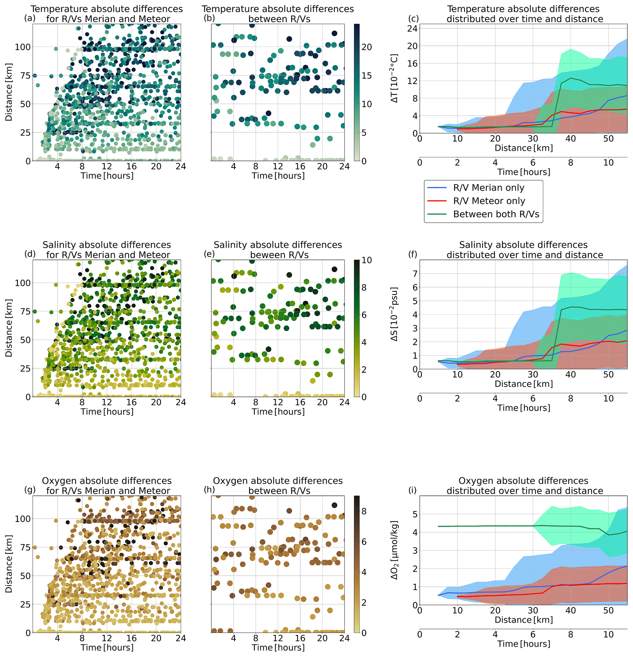
Figure 4 displays the difference between the two calibration methods applied to the R/V L'Atalante CTD profiles. For each parameter, most of the differences are found within the range of the sensor's accuracy, as provided by Sea-Bird. For temperature, differences range between −0.7 and 0.25 ^∘C, with a mean difference of $-\mathrm{3}\times {\mathrm{10}}^{-\mathrm{3}}$ ^∘C and a median difference of $-\mathrm{6}\times {\mathrm{10}}^{-\mathrm{4}}$ ^∘C. In Fig. 4d, we observe that the highest differences are situated between 50 and 250 m depth, which is within the thermocline. For salinity and oxygen, the distributions of the differences are found to be within the accuracy of the sensors, and the median and mean difference are close to zero. However, Fig. 4d shows that, at the base of the mixing layer, a salinity difference is sizable and amounts up to 0.3 psu. These differences, although minimal, raise the question of whether CTD validation and calibration follow the best practices. Both IFREMER and GEOMAR follow the recommendations from GO-SHIP in terms of CTD deployment and calibration. However, we observe that slight differences in the procedures can lead to non-negligible differences when the vertical gradients are more pronounced. Below these depths, the different approaches showed no major discrepancies, as the differences are inferior to the accuracy of the sensors.

In general, at each isopycnal level, the differences between two profiles with small temporal and spatial separations can be linked to two sources, namely the different calibration procedures and internal ocean variability. As the IFREMER and GEOMAR CTD calibration procedures provide similar results around the same order of magnitude as the accuracy of the sensors, the remaining differences between the various datasets must be primarily due to the ocean variability. Figure 5a and b present the salinity absolute differences on isopycnal level for each R/V and for CTD profiles found within a specific distance and time, respectively. As observed here, the averaged salinity differences, and associated standard deviation, depend on the density. The largest variations are particularly noticeable on isopycnal levels within which NBC rings evolve and for denser water masses that were sampled less frequently during the EUREC⁴A-OA field experiment. Moreover, as expected, these differences increase with time and distance (see Fig. 5c and d for the vertically averaged absolute salinity differences), independently of the area of deployment. R/V L'Atalante displays higher variability compared to R/Vs Maria S. Merian and Meteor, which is mostly linked to the different areas observed. The variability more than doubles for CTD profiles more than 25 km away or undertaken more than 4 h apart. This illustrates the importance, for intercalibration purposes, of focusing on close-by pairs of profiles.

The calibrated CTD dataset for each R/V is associated with an uncertainty for every parameter. However, the creation of an assembled dataset gathering all profiles requires a comparison of these arrays. Figure 6 displays the vertically averaged differences for each parameter. The calculations are made on isopycnal levels. The left column shows these differences for the profiles performed by the same R/V as a function of both time and distance, which are also represented by the blue and red curves in the right panels. These curves exhibit the oceanic variability plus the post-calibration uncertainty; for nearby CTD pairs, they tend towards this last value. The central column of Fig. 6 represents the difference calculated with one CTD profile from each R/V that is synthesized by the green curves in the right panels. These curves are the result of both oceanic variability and uncertainty linked to the differences in deployment and calibration between each R/V and the laboratory. For all the measured parameters, these differences are found between those calculated for an individual R/V, on average, and the standard variability. This indicates that the uncertainty remains low in terms of the order of magnitude (equivalent to that provided by the laboratory calibration). The same comparison performed between the CTD profiles acquired by R/Vs Maria S. Merian and Meteor is shown in Fig. 7. These profiles show small differences in temperature and salinity but remain within the standard deviation of the differences computed for the profiles acquired by the individual R/V. This is expected, since the CTD temperature and conductivity profiles undertaken by R/V Meteor are calibrated using close-by CTD profiles acquired by R/V Maria S. Merian. The resulting uncertainties for the R/V Meteor temperature and salinity profiles are $\mathrm{2}\times {\mathrm{10}}^{-\mathrm{2}}$ ^∘C and $\mathrm{5}\times {\mathrm{10}}^{-\mathrm{3}}$ psu, respectively, and this is for three pairs of profiles found less than 5 km apart. Nevertheless, for dissolved oxygen, this difference is of 4 µmol kg⁻¹, which is about the same order of magnitude as 5 µmol kg⁻¹ found for the uncertainty linked to the different calibration procedures.

3.3 Ship intake water analysis

3.3.1 Thermosalinograph

R/Vs L'Atalante and Meteor are equipped with Sea-Bird SBE21 TSGs, and R/Vs Maria S. Merian and Meteor used two Sea-Bird SBE45 TSGs. These devices continuously measure temperature and salinity near the surface, between 6 and 7 m depth, depending on actual ship draft. The measurements are made at a frequency of 1 Hz and then averaged in 2 min bins. Each day, for R/Vs Maria S. Merian and L'Atalante, a water sample is taken and analyzed aboard in order to adjust the salinity measurements. Figure 8 shows the positions of the TSG records during the EUREC⁴A-OA experiment.

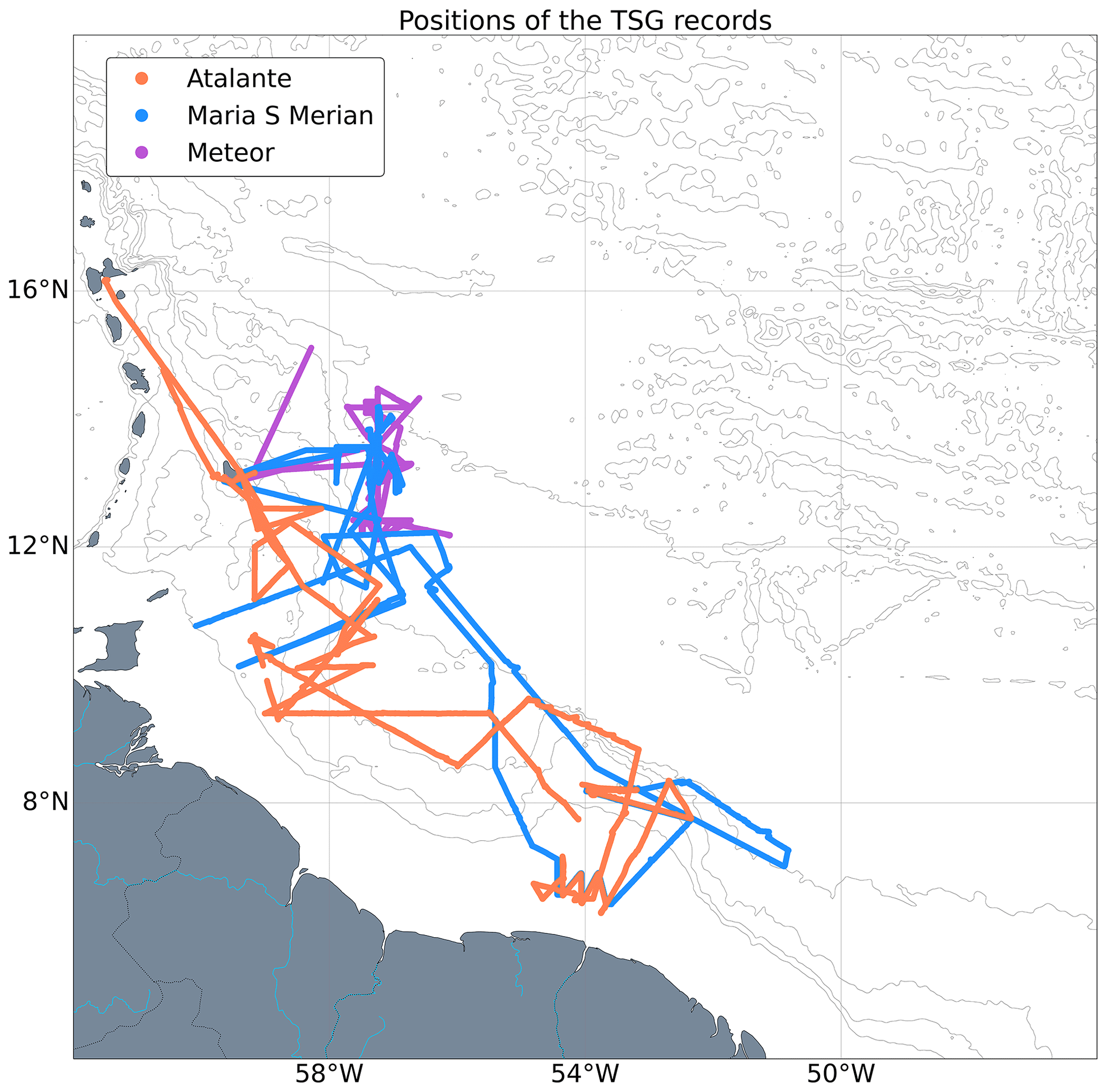
Figure 8 Map of the TSG records performed by R/Vs L'Atalante, Maria S. Merian, and Meteor.

As the measurements from this device are compared and corrected with actual water samples measured with level 1 sensors on R/Vs L'Atalante and Maria S. Merian, the calibrated TSG records are at level 2 of our calibration hierarchy. For R/V Meteor, the level is set at 3 for the salinity measurements.

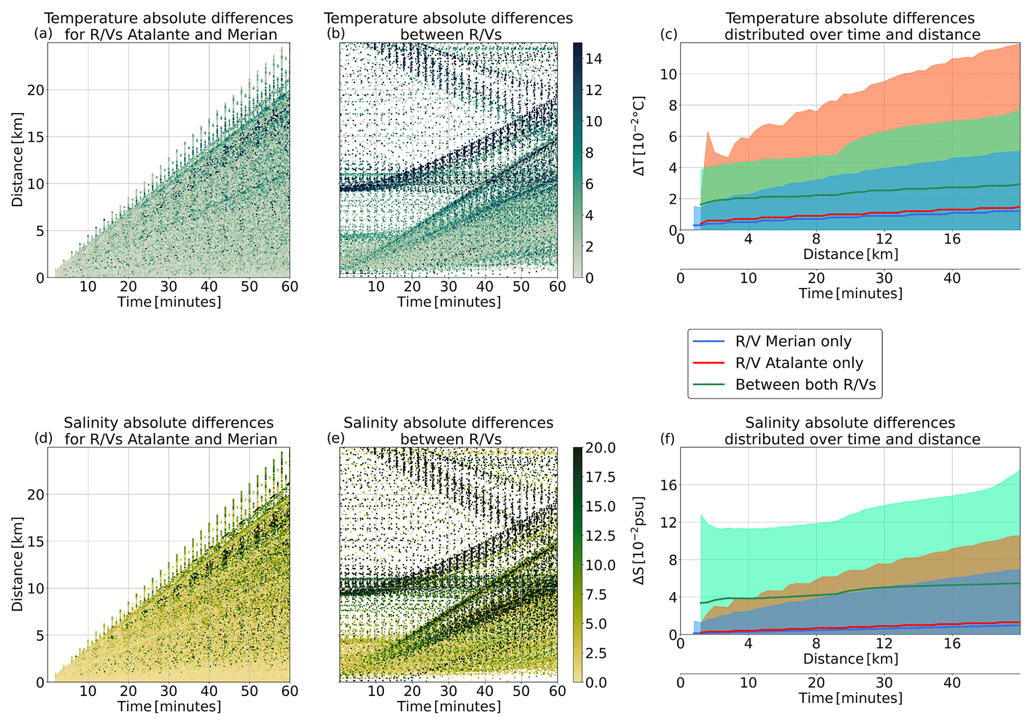
Figure 9 (a) Absolute temperature differences between TSG pairs of measurements distributed in time and distance. Each TSG pair is only composed of measurements from R/Vs L'Atalante or Maria S. Merian. (b) Same as panel (a) but for TSG pairs composed of one measurement from R/V L'Atalante and one from R/V Maria S. Merian. (c) Temperature differences as a function of time and distance for CTD pairs from R/Vs Maria S. Merian (blue) and L'Atalante (red) and composed of one profile of each (green). Panels (d), (e), and (f) are same as above but for absolute salinity differences.

The absolute differences for surface temperature and salinity, calculated from the TSG, are displayed in Fig. 9. Compared to the CTD measurements (see Figs. 6 and 7), the TSG resolution allows for finer spatiotemporal scales of observations. R/Vs L'Atalante and Maria S. Merian captured, on average, the same absolute differences for both temperature and salinity, while R/V L'Atalante presents a larger standard deviation. Nevertheless, the difference calculated between the two ships remains on average around $\mathrm{2}\times {\mathrm{10}}^{-\mathrm{2}}$ ^∘C and $\mathrm{4}\times {\mathrm{10}}^{-\mathrm{2}}$ psu above the ones calculated for each individual R/V. Similar offsets are found for R/V Meteor (not shown). For temperature, the standard deviation of the difference calculated between the TSG of each R/V remains in the same range as the ones obtained for individual TSGs, but for salinity, it exceeds the individual TSG ranges. These differences can be attributed to the calibration processes, to the differences between the two TSG types, and to the background oceanic variability. Overall, the TSG ensemble from all R/Vs is used for comparison with other devices measuring the surface, with a traceability of level 3 or below.

3.4 Underway platforms

3.4.1 Underway CTD (uCTD)

An Oceanscience underway CTD system was used on R/Vs L'Atalante and Maria S. Merian. The uCTD consists of a small winch system mounted on the bulwark of the ship and a CTD probe measuring temperature, conductivity, and pressure (Rudnick and Klinke, 2007). The probes sample at 16 Hz, and data are recorded internally and read out on board via a Bluetooth connection. This probe is designed to record data during descent, and the deployment procedure minimizes the influence of surface waves. The uCTD can be used in free-cast and tow-yo (or free-fall) modes, depending on whether a winding line is spooled (or not) onto the tail. In the first case, the probe descent is decoupled from the winch spool friction, keeping a rather steady descent rate of about 4 dbar s⁻¹. In the second mode, the probe fall rate is determined by the idle friction of the spool and the probe friction, and descent may vary between 3.5 and about 0.6 dbar s⁻¹. For deployments of the uCTD from R/V Maria S. Merian, both modes were used, with the tow-yo mode preferred for water depths shallower than 500 m. For deployments from R/V L'Atalante, the uCTD was only deployed using the free-fall mode, with no line spooled onto the tail. The difference in descent rate is an important factor to take into account in the calibration procedure, as the water is not pumped toward the sensors, contrary to what happens for sensors mounted on the CTD.

R/V Maria S. Merian acquired a total of 380 profiles, using three different uCTD probes, and this was usually performed in series with a drop every 30 min. R/V L'Atalante carried out 179 uCTD profiles using two probes and usually alternating their deployment with CTD profiles. Figure 10a shows the positions of these profiles. Depending on the ship speed, the uCTDs sampled the water column between the surface and 300 to 500 m depth. Because no real-time information on the actual depth of the probe is available, the operator has to estimate the probe depth via cast time and estimated sinking velocity.

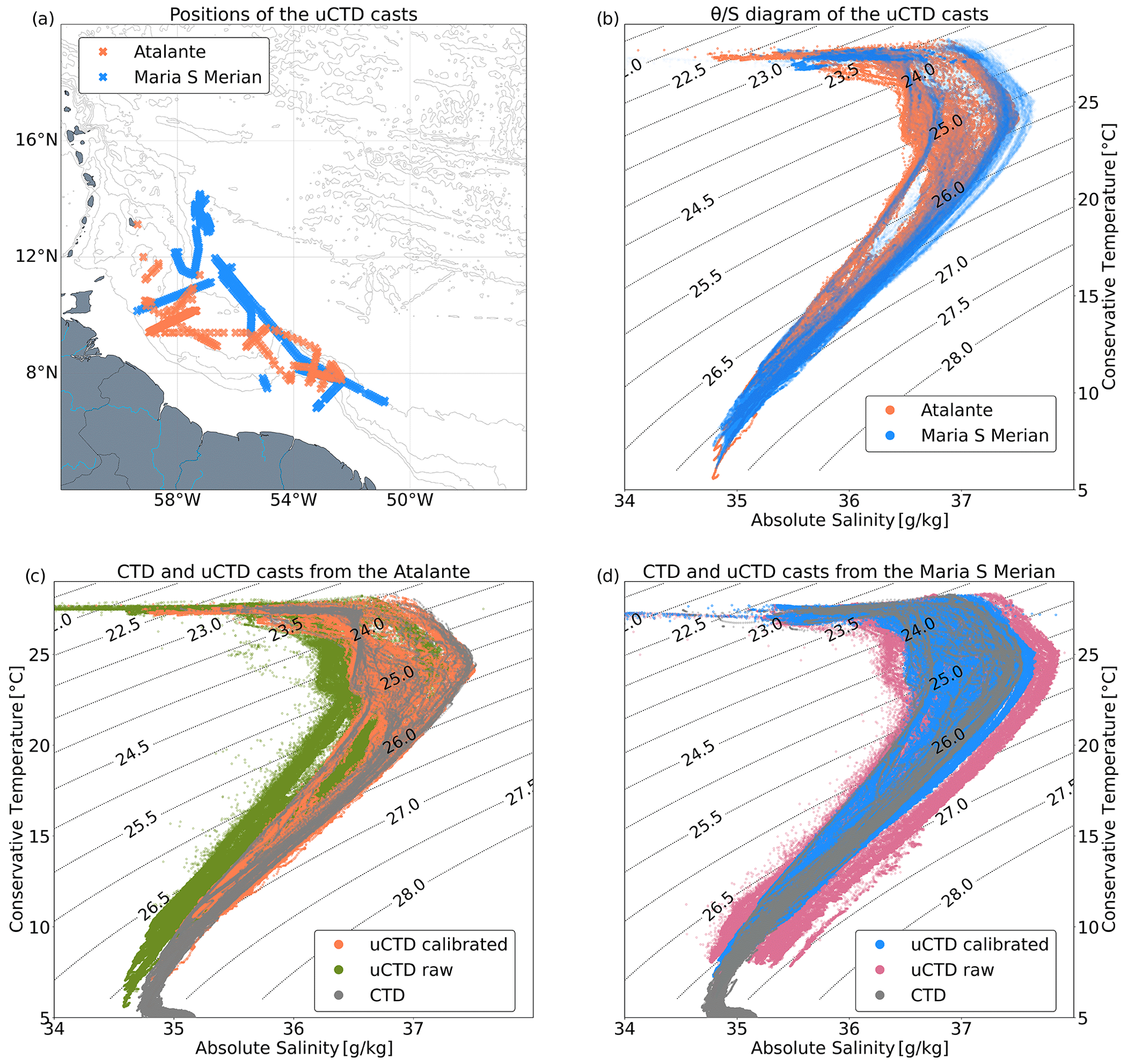
Figure 10 (a) Map of the uCTD cast positions for R/Vs L'Atalante and Maria S. Merian. (b) θ/S diagram of the uCTD-calibrated profiles for each ship superimposed on the isopycnals. Panels (c) and (d) show a comparison of the raw and calibrated uCTD profiles superimposed on the CTD profiles for R/Vs L'Atalante and Maria S. Merian, respectively.

There are four sources of salinity uncertainty associated with the uCTD measurements, leading to errors of about 4–5 $\times {\mathrm{10}}^{-\mathrm{3}}$ ^∘C and resulting in a computed salinity error of 4–5 $\times {\mathrm{10}}^{-\mathrm{3}}$ psu (Ullman and Hebert, 2014). The first arises from a looping of the probe, during which its direction reverses. The uCTD is made to only record data during descent so that periods of inverse descent rate can be easily removed during the validation procedure. The second source of error comes from the variable fall rate of the probe. As the water is not pumped towards the sensors, there can be a lag in the measurements linked to the time it takes for the parcel of water to pass from one sensor to the other (Perkin et al., 1982; Lueck, 1990). Corrections are achieved via a minimization of this temporal lag, which depends on the fall rate. The third source of error is related to the high deceleration of the probe when the spooled line reaches its end, leading to viscous heating of the thermistor. Larson and Pedersen (1996) provide a correction for this effect that is taken into account before computing salinity. The final source of error for salinity is detected as staggered changes when comparing the CTD profiles to those of the uCTD. Indeed, salinity values are lower for the uCTD than for CTD profiles when the temperature increases. This conductivity cell thermal mass error has been described in Lueck (1990), and Lueck and Picklo (1990) proposed a correction based on the calculation of two parameters, namely the magnitude of the error α and a time constant of the error τ.

To perform the thermal mass correction, it is necessary to have close-by CTD/uCTD profiles. Specific profiles were also undertaken with the uCTD probe directly attached to the CTD rosette to gather the most synoptic measurements possible. Nevertheless, while the uCTD is designed to record the water column in a free-fall mode, with the probe attached, it is lowered at a constant but lower speed, and the presence of the rosette can disturb the flow near the sensor intake. As a consequence, even the co-located uCTD-CTD profiles can underestimate the error.

All corrections are performed using a MATLAB toolbox based on Ullman and Hebert (2014). The procedure uses two separate calibrations, namely direct calibration of the uCTD probe attached to a CTD, giving nearly collocated uCTD and CTD profiles, and comparison with the TSG salinity. Figure 10b shows the calibrated profiles, and Fig. 10c and d present their comparisons with CTD and raw uCTD profiles for each ship.

Figure 11 (a) Absolute temperature differences between CTD/uCTD pairs of profiles on isopycnal levels and averaged vertically distributed in time and distance. Each pair is composed of profiles from the same R/V (one CTD and one uCTD). (b) Temperature differences as a function of time and distance for pairs of profiles from R/V Maria S. Merian. The differences are given in blue for pairs of CTD-only profiles, in red for pairs composed of one CTD and one uCTD profile, and in green for pairs composed of one CTD and one uncalibrated uCTD profile. Panel (c) is the same as (b) but for R/V L'Atalante. Panels (d), (e), and (f) are the same as above but for absolute salinity differences.

For the corrected uCTD, some calibration profiles were performed with the uCTD probe attached to the CTD rosette, while others were calibrated by comparing to nearby CTD stations. Both of these methods rely on comparing the uCTD profiles with close-by and sometimes synoptic CTD profiles and are thus assigned to level 3 in our calibration hierarchy. After the correction of the uCTD data, we observe a clear improvement and agreement between the CTD and uCTD profiles. Figure 11 shows the vertically averaged differences between CTD and uCTD measurements for temperature and salinity for each individual R/V. Since the uCTD is calibrated with nearby CTD profiles, it is particularly interesting to notice that the correction highly reduces the differences in both temperature and salinity for the mean and standard deviation, leading them closer to the differences measured by only the CTD. For R/V L'Atalante, the comparison matches better than for R/V Maria S. Merian, which is possibly linked to the deployment strategy, where uCTD and CTD measurements were alternately cast for R/V L'Atalante, increasing the number of profiles to use as references for calibrations, while for R/V Maria S. Merian, only full sections used uCTD casts. The difference between the CTD-only curve and the one combining CTD and uCTD provides an estimation of the uncertainty of $\mathrm{9}\times {\mathrm{10}}^{-\mathrm{2}}$ ^∘C and $\mathrm{2}\times {\mathrm{10}}^{-\mathrm{2}}$ psu for both ships, with five pairs of profiles found within 10 km and 2 h for R/V Maria S. Merian and 10 pairs for R/V L'Atalante.

3.4.2 Moving Vessel Profiler (MVP)

A Moving Vessel Profiler (MVP30–350) from AML was operated on R/Vs L'Atalante and Maria S. Merian. The MVP allows underway measurements from the surface down to a depth that depends highly on the ship and water current speed, reaching a maximum of 350 m. The MVP30–350 consists of an electric winch system, a PC control unit, and a towed vehicle (fish) that can be equipped with different sensors. A conductive probe provides real-time data access. The fish is forced to rapidly (up to 2 m s⁻¹) descend and ascend with the help of a tail unit. The fish design enables descent, ascent, and drag-phase (time before the next descent) data recordings to be used.

The MVP deployed from R/V Maria S. Merian performed 1891 profiles, with ship speed from 2 to 10 kn (mean 6.9 kn). The MVP deployed from R/V L'Atalante completed 1960 profiles (Fig. 12a). The device was operated in different areas and guided by dynamical features (mesoscale eddies, filaments, and frontal regions). In regions with a shallow topography, the maximal diving depth was either controlled by an operator (real-time data) or by feeding the bottom topography (e.g., from the echo sounder of the ships) into the MVP control unit (as done on R/V Maria S. Merian in shallow topography and requesting the fish to ascend when reaching a depth of 10 m above the seafloor). On R/V Maria S. Merian, the MVP was also equipped with a fluorescence sensor.

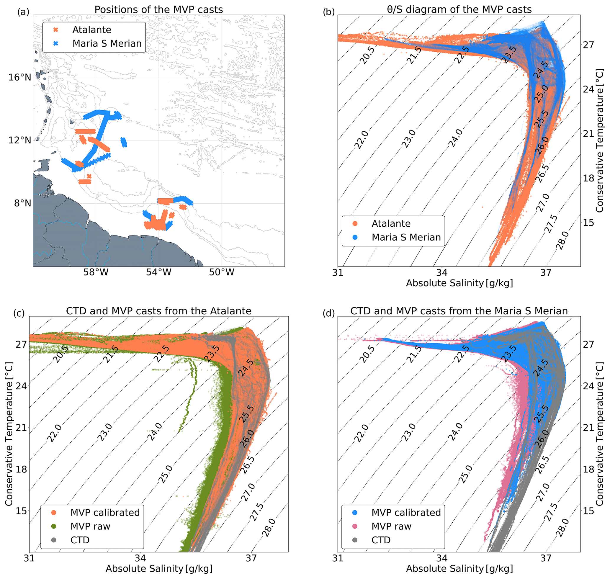
Figure 12 (a) Map of the MVP cast positions for R/Vs L'Atalante and Maria S. Merian. (b) θ/S diagram of the MVP-calibrated profiles for each ship superimposed on the isopycnals. Panels (c) and (d) show the comparison of the raw and calibrated MVP profiles superimposed on the CTD profiles for R/Vs L'Atalante and Maria S. Merian, respectively.

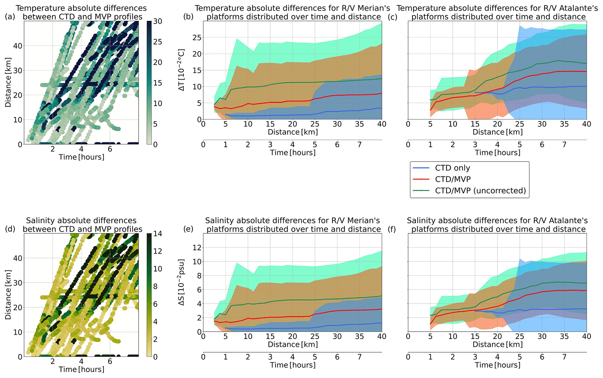
Figure 13 (a) Absolute temperature differences between CTD/MVP pairs of profiles on isopycnal levels, averaged and vertically distributed in time and distance. Each pair is composed of profiles from the same R/V (one CTD and one MVP). (b) Temperature differences as a function of time and distance for pairs of profiles from R/V Maria S. Merian. The differences are given in blue for pairs of CTD-only profiles, in red for pairs composed of one CTD and one MVP profile, and in green for pairs composed of one CTD and one uncalibrated MVP profile. Panel (c) is the same as (b) but for R/V L'Atalante. Panels (d), (e), and (f) are the same as above but for absolute salinity differences.

The CTD sensors on the MVP are affected by similar sources of error as the uCTD (i.e., the speed of the probe through the water, conductivity and temperature time lag, and thermal mass), and a similar calibration strategy is therefore used for the MVP sensors. The MVP also appears to be sensitive to surface waves. We therefore removed them by applying a low-pass filter with a cutoff frequency calculated from the surface waves of 0.2 Hz. As explained in the uCTD section, the temporal lag and thermal mass errors are linked, respectively, to the vertical speed and the time match between conductivity and temperature pairs. In order to perform this calibration, we calculated downward and upward correction coefficients, based on the method of Mensah et al. (2018). The calibration resulted in a good match between nearby ship CTD and CTD sensors on the MVP (Fig. 12c, d).

Because the calibration only takes into account the nearby CTD profiles, temperature, salinity, and pressure measurements are ranked level 3 for traceability. We observe (Fig. 13) that the averaged differences between nearby CTD profiles and standard deviations reduce after calibration. As for the uCTD comparisons with the CTD, a difference between CTD-only and MVP/CTD profiles subsist. Again, this is attributed to the different deployment of the devices, the sampling strategy, and the oceanic variability in the regions measured. The estimated uncertainty for the corrected MVP is of $\mathrm{3}\times {\mathrm{10}}^{-\mathrm{2}}$ ^∘C, and $\mathrm{1}\times {\mathrm{10}}^{-\mathrm{2}}$ psu for R/V L'Atalante and $\mathrm{4}\times {\mathrm{10}}^{-\mathrm{2}}$ ^∘C, and $\mathrm{2}\times {\mathrm{10}}^{-\mathrm{2}}$ psu for R/V Maria S. Merian, with, respectively, 10 and 70 pairs of profiles found within 5 km and 1 h.

3.5 Ship-mounted ADCP (S-ADCP)

Upper-ocean currents were measured quasi-continuously with Teledyne RD Instruments acoustic Doppler current profiler (S-ADCP). On all three ships, a 38 kHz ADCP was operated, measuring velocities from around 50 to sometimes even below 1000 m depth, depending on the availability of scatters. R/Vs Meteor and Maria S. Merian were also equipped with a 75 kHz ADCP, providing measurements between 40 and 800 m depth, with a finer resolution compared to the 38 kHz S-ADCP. R/V L'Atalante, on the other hand, was equipped with a 150 kHz ADCP, supposedly ranging from around 20 to 400 m depth. However, this ADCP rarely reached water depths below 200 m during the experiment. The ADCP accuracy is ±5 % of the measured velocity or ±0.5 cm s⁻¹ – whichever is greater.

During the experiment, on a daily basis, data from R/V L'Atalante were then processed with the CASCADE software developed by IFREMER (Le Bot et al., 2011; Speich et al., 2021b). The data from R/Vs Maria S. Merian and Meteor were processed using a set of MATLAB routines applied to the raw data, meaning that the data were sampled in an as-fast-as-possible mode (approximately 1 Hz).

To enable a direct comparison of the measurements from all ships, the ADCP data were reprocessed using the UHDAS routines Firing et al. (2012). This comparison did not show any notable difference among the datasets. The final dataset consists of zonal and meridional velocities averaged in 2 min segments. As the device is directly mounted on the hull of the ships, the measurements follow the same tracks as the TSG (Fig. 8).

By default, we place the processed S-ADCP measurements on the second level of our hierarchy, since only an intercomparison between devices can be done, and no comparison with a reference is possible. The L-ADCP measurements are placed one level below (level 3), since the S-ADCP measurements are used as a reference.

4 Autonomous devices

4.1 Underwater gliders

4.1.1 Pressure, temperature, conductivity, and salinity

During the experiment, seven underwater gliders were deployed (Fig. 14). From R/V L'Atalante, a SeaExplorer glider, named Kraken, was deployed and carried out 831 profiles to a maximum depth of 700 m in 15 d of operation. The glider was deployed to cross along different quadrants of a mesoscale eddy previously located in satellite altimetry maps. Its CTD, a glider payload CTD (GPCTD) has an accuracy of $\mathrm{4}\times {\mathrm{10}}^{-\mathrm{3}}$ ^∘C for temperature and $\mathrm{1}\times {\mathrm{10}}^{-\mathrm{3}}$ mS cm⁻¹ for conductivity (as claimed by the manufacturer).

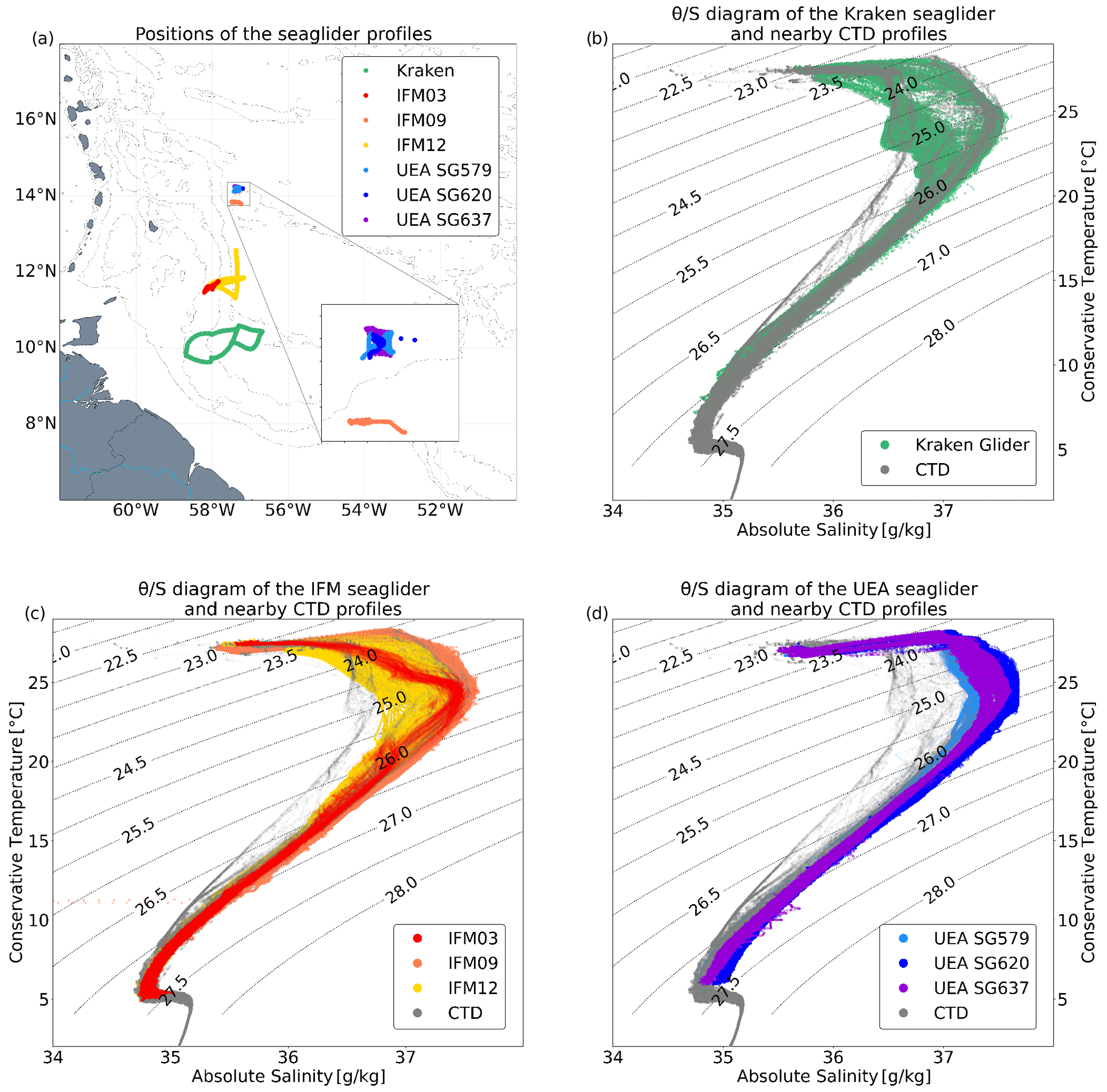
Figure 14 (a) Map of the seven underwater glider positions. (b) θ/S diagram of the Kraken glider measurements, deployed from R/V L'Atalante, compared to nearby CTD casts. (c) Same as panel (b) but for the IFM gliders deployed from R/V Maria S. Merian. (d) Same as panel (b) but for the University of East Anglia gliders deployed from R/V Meteor.

From R/V Maria S. Merian, three autonomous gliders (IFM03, IFM09, and IFM12, where IFM stands for Institut für Meereswissenschaften, the Leibniz Institute of Marine Sciences in Kiel, Germany) were deployed. IFM09 conducted 327 profiles to a maximum depth of 900 m in 20 d, following a quasi-stationary mode in the trade wind alley area. IFM03 and IFM12 were deployed in the northeastern region of a mesoscale eddy, performing, respectively, 125 and 443 profiles down to a maximum depth of 900 m in 6 and 24 d, respectively. Due to a leak, IFM03 was retrieved by R/V Meteor.

Three gliders from the University of East Anglia (UEA) collected profiles with an hourglass sampling pattern. The gliders (SG579, SG620, and SG641) collected 442, 262, and 308 profiles for 10, 13, and 24 d down to maximum depths of 950, 750, and 750 m, respectively.

The IFM and UEA gliders were equipped with unpumped SBE41 Sea-Bird CTDs (Stevens et al., 2021), with a manufacturer accuracy of $\mathrm{2}\times {\mathrm{10}}^{-\mathrm{3}}$ ^∘C for temperature and $\mathrm{3}\times {\mathrm{10}}^{-\mathrm{3}}$ mS cm⁻¹ for conductivity. The underwater gliders are subject to the same sources of errors as all the previously described undulating probes. Nevertheless, the rising and descending profiles are performed at a much lower speed compared to the free-fall of the uCTD. For Kraken, the water was pumped through the CTD, and this controlled flow highly diminished the viscous heating and temporal lag effects. For the other underwater gliders, this was not the case, and the flow speed was estimated by determining the speed of movement through the water, based on an optimized glider travel model.

In principle, similar correction procedures were used for the MVP and underwater gliders. These were necessary to avoid any misalignment between the downward and upward profiles, taking into account the flight model, and to have coherent calibrations across the platforms.

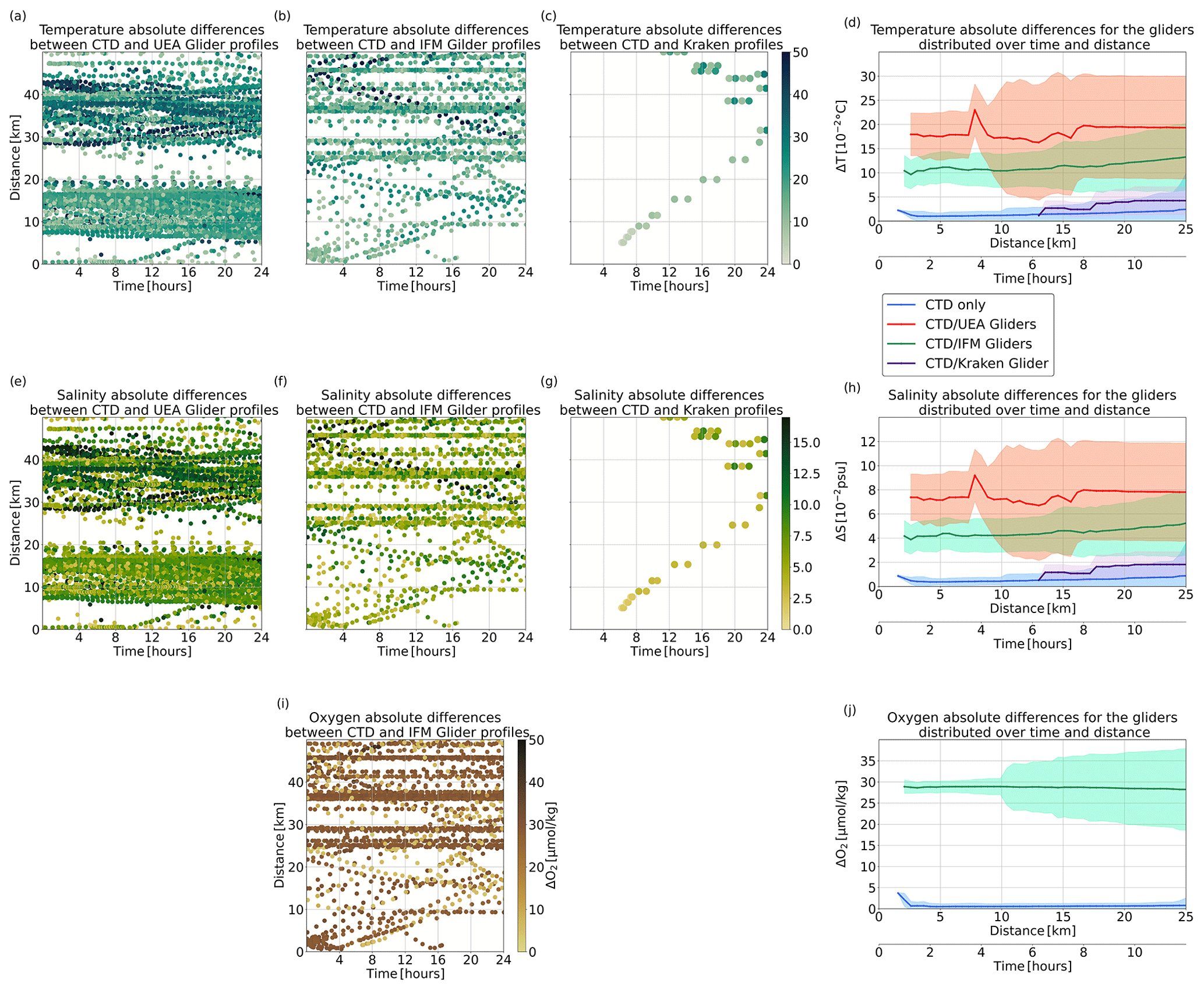
Figure 15 Panels (a), (b), and (c) show the temperature absolute differences between CTD/glider pairs of profiles on isopycnal levels, averaged and vertically distributed in time and distance. Each pair is composed of one CTD and one glider profile. Respectively, panels (a), (b), and (c) correspond to the UEA, IFM, and Kraken gliders. (d) Temperature differences as a function of time and distance for pairs of profiles. The differences are shown in blue for pairs of CTD-only profiles, in red for pairs composed of one CTD and one UEA profile, in green for pairs composed of one CTD and one IFM profile, and in purple for pairs composed of one CTD and one Kraken profile. The middle line of panels (e) to (h) is the same as above but for salinity absolute differences. The bottom line of the panels correspond to oxygen absolute differences, but only IFM gliders measured dissolved oxygen.

No direct or lab calibration was done with the glider CTD sensors; instead, data calibration was performed through comparison with nearby (time and space) CTD stations. To ease comparison, we group all three gliders (UEA Seaglider, the IFM gliders, and the Kraken; Fig. 15, above and middle line panels). The number of close-by pairs of CTD and glider profiles is quite low for the Kraken. Nevertheless, the mean differences for the pairs of profiles found to be closer than 15 km (with 15 pairs of profiles) are less than $\mathrm{3}\times {\mathrm{10}}^{-\mathrm{2}}$ ^∘C and $\mathrm{1}\times {\mathrm{10}}^{-\mathrm{2}}$ psu. The IFM gliders tend to a constant positive bias in temperature and salinity compared to the nearby CTD stations, with a low standard deviation, despite having a higher number of pairs of profiles. Within the first 10 km (about 60 pairs of profiles), the uncertainty is of the order of 0.1 ^∘C and $\mathrm{4}\times {\mathrm{10}}^{-\mathrm{2}}$ psu. The UEA Seaglider shows higher differences in temperature and salinity associated with a large standard deviation. These values can not only be attributed to the calibration and differences between devices but also to the sampling strategy; the pairs UEA Seaglider/CTDs are mostly associated with R/V Meteor stations (more than 140 pairs of profiles within the first 10 km; see Fig. 3a), where the salinity has not been calibrated with a direct comparison with water samples. This probably impacts the resulting isopycnal levels, where the absolute difference is calculated. Their uncertainty is estimated here at $\mathrm{1.8}\times {\mathrm{10}}^{-\mathrm{1}}$ ^∘C and $\mathrm{7}\times {\mathrm{10}}^{-\mathrm{2}}$ psu. As for the MVP measurements, the underwater gliders compared to the CTD profiles from R/Vs Maria S. Merian and L'Atalante are placed at level 3 on the calibration hierarchy. The UEA gliders are principally compared with CTD profiles acquired by R/V Meteor and thus placed one level below.

4.1.2 Dissolved oxygen

The three IFM gliders were equipped with AADI Aanderaa optodes of type 3830 (IFM03 and IFM09) and type 4831 (IFM12). The manufacture-provided resolution and accuracy for oxygen concentration are 1 mmol and 8 M or 5 % (whichever is greater; concentration) and <5 % (air saturation). For the three IFM gliders, lab calibrations of the oxygen sensors were done on board the Maria S. Merian by preparing 0 (chemically forced) and 100 % saturation (air bubbles injected) water of two temperatures, following the Aanderaa optode manual. The resultant readings were used to constrain the phase $/$ temperature relation of the foil.

Figure 15j provides information about the oxygen concentration with, on average, negative (not shown) differences of 28 µmol kg⁻¹. However, this relatively high uncertainty value has to be put in perspective with the associated standard deviation of about ±2 µmol kg⁻¹ for CTD/glider pairs found within 10 km. This uncertainty has the same order of magnitude as the sensor accuracy, suggesting a rather constant bias in the sensors. The oxygen, as measured by the IFM gliders, is placed at level 3 of the calibration hierarchy.

Figure 16 Map of the five Saildrone positions. Three NASA Saildrones (1026, 1060, and 1061) and one NOAA Saildrone (1063) have followed R/Vs Maria S. Merian and L'Atalante tracks to sample surface mesoscale eddies, while one NOAA Saildrone (1064) has first sampled the trade wind alley.

4.1.3 Other sensors

CDOM optical sensors were mounted on the IFM12, SG579, and Kraken gliders to estimate dissolved organic matter. A submersible underwater nutrient analyzer (SUNA) was used on IFM12. IFM03 and SG620 were equipped with a Rockland Scientific MicroRider turbulence sensor to estimate small-scale mixing. The SG637 glider was equipped with a Nortek Signature1000 1 MHz ADCP to measure the vertical shear of horizontal currents. None of these sensors is considered here.

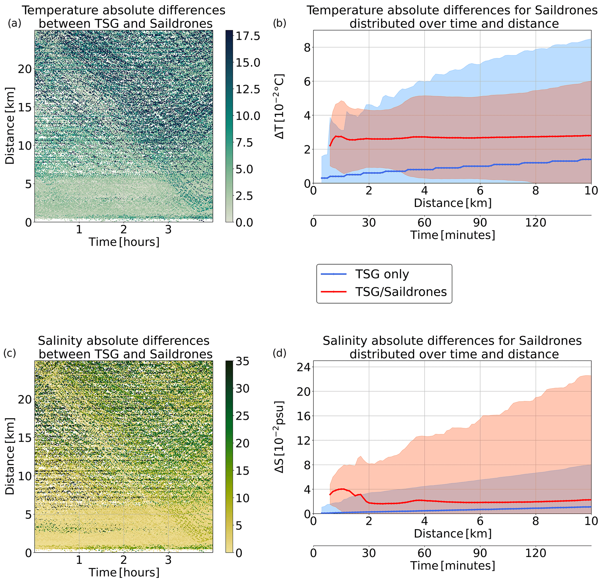
Figure 17 (a) Absolute temperature differences between TSG/Saildrone pairs of measurements distributed in time and distance. Each pair is composed of one R/V's TSG measurement and a Saildrone one. (b) Temperature differences as a function of time and distance for a pair of surface measurements. Differences are given in blue for pairs of R/V TSG-only profiles and in red for pairs composed of one R/V TSG and one Saildrone. Panels (c) and (d) are same as above but for absolute salinity differences.

4.2 Saildrones

With the objective of measuring the ocean–atmosphere interface, five Saildrones were deployed from Barbados, with three funded by NASA and two by NOAA (see Fig. 16). Below the water line, a pumped CTD (SBE-37-SMP-ODO MicroCAT) measured temperature, conductivity, and dissolved oxygen at 0.5 m depth, and they were also equipped with a chlorophyll a sensor (WETLabs ECO-FL-S G4 and Turner Cyclops). A Teledyne Workhorse 300 kHz ADCP was mounted on the NASA Saildrones to measure the current velocity from 6 to 100 m depth. Their nominal accuracies are $\pm \mathrm{2}\times {\mathrm{10}}^{-\mathrm{3}}$ ^∘C for temperature, $\pm \mathrm{3}\times {\mathrm{10}}^{-\mathrm{3}}$ mS cm⁻¹ for conductivity, ±3 µmol kg⁻¹ or ±2 % for dissolved oxygen, and $\mathrm{2}\times {\mathrm{10}}^{-\mathrm{2}}$ µg L⁻¹ for chlorophyll a. These values have the same order of magnitude as those for the sensors mounted on the CTD probes. The ADCP accuracy is ±5 % of measured velocity or ±0.5 cm s⁻¹, which is similar to that of the S-ADCPs. The Saildrones are autonomous and operated remotely, and their measurements are valuable, as they provide 1 min averaged records of temperature and salinity near the sea surface and 5 min averaged records of velocity, with a high vertical resolution in the upper layer of the water column. Nevertheless, calibrations were only made in the laboratory before and after the mission, as direct comparisons with water samples are impossible; as such, we place the Saildrones on level 3 of our calibration hierarchy.

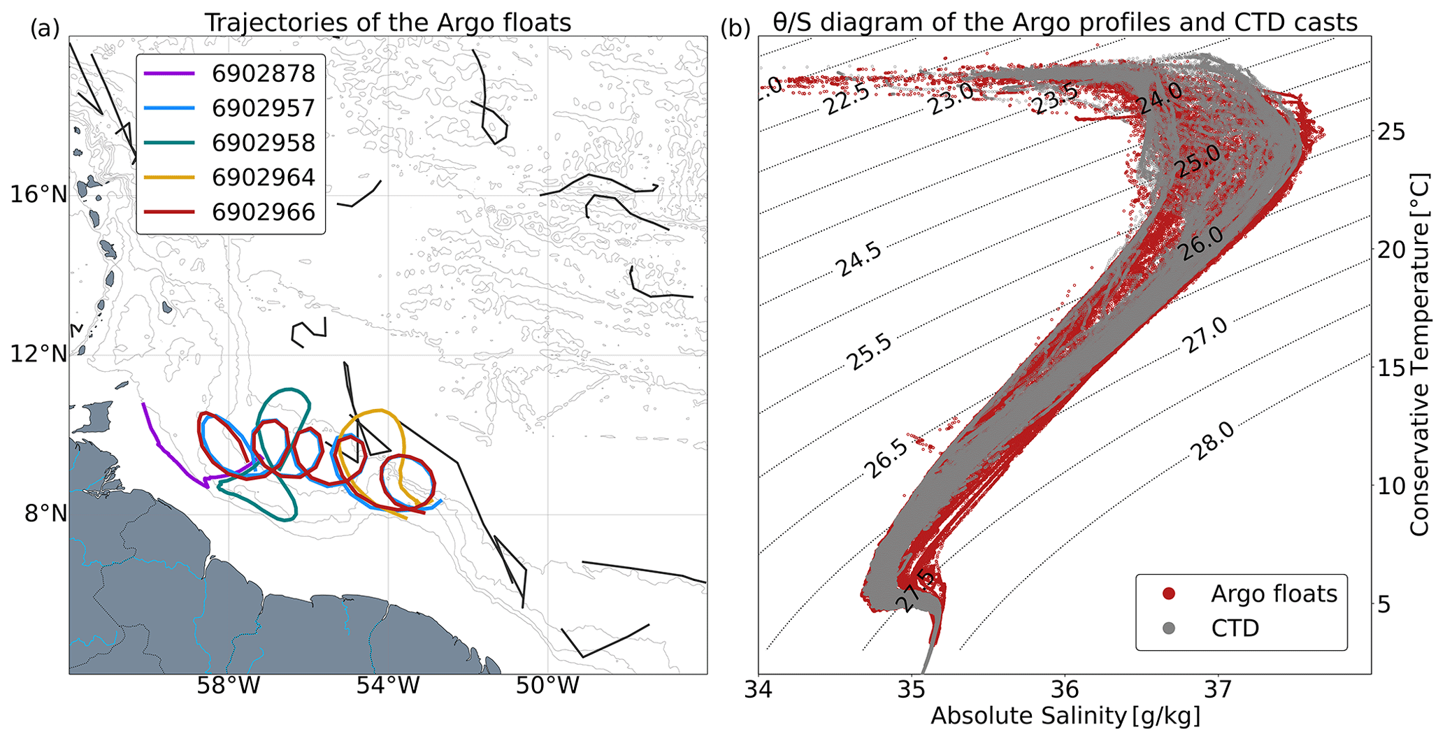
Figure 18 (a) Map of the Argo floats found in the region of interest between December 2019 and May 2020; specific colors are attributed to the five floats deployed from R/V L'Atalante. (b) θ/S diagram of the Argo floats, compared to nearby CTD casts. No clear bias is observed here.

As for the previous devices, Fig. 17 shows the comparison between the temperature and salinity measurements made by the Saildrones and the near-surface values from R/Vs L'Atalante and Maria S. Merian measurements. The Saildrones followed their own routes away from the ships; nevertheless, the high frequency of acquisition provides enough nearby measurements for comparison. For calibration purposes, four of the five Saildrones spent times near R/V L'Atalante on two occasions. For temperature, measurements were found below 1 km apart, and more than 350 pairs of measurements were less than 1 km apart. The resulting difference is of the order of $\mathrm{2.5}\times {\mathrm{10}}^{-\mathrm{2}}$ ^∘C. For salinity, the absolute difference climbs to $\mathrm{4}\times {\mathrm{10}}^{-\mathrm{2}}$ psu for measurements found less than 1 km apart. This difference reduces to $\mathrm{1}\times {\mathrm{10}}^{-\mathrm{2}}$ psu when using the R/Vs TSG tendency.

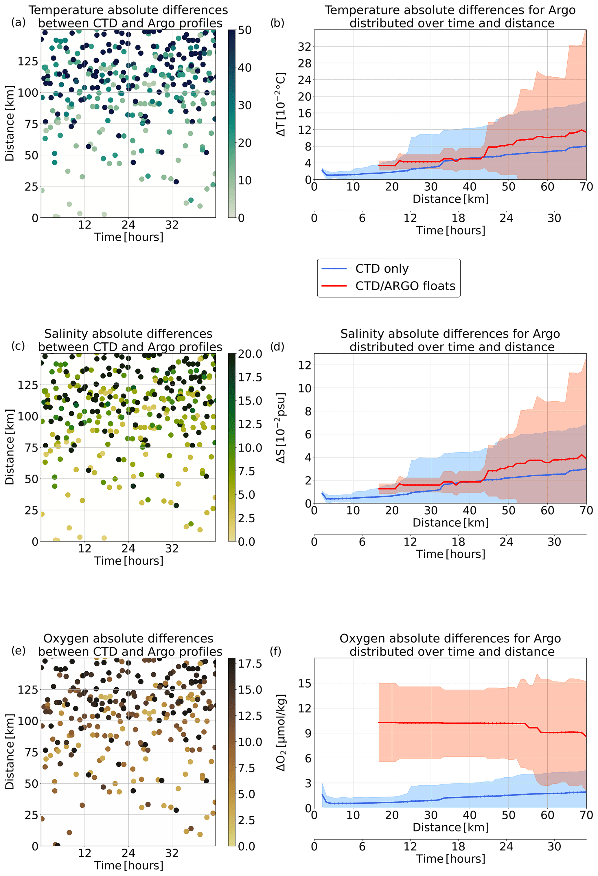
Figure 19 (a) Absolute temperature differences between CTD/Argo float pairs of profiles on isopycnal levels, averaged and vertically distributed in time and distance. Each pair is composed of one CTD and one Argo float profile. (b) Temperature differences as a function of time and distance for pairs of profiles. Differences are shown in blue for pairs of CTD-only profiles and in red for pairs composed of one CTD and one Argo float profile. The middle line of panels is the same as above but for absolute salinity differences. The bottom line of panels corresponds to absolute oxygen differences.

4.3 Argo floats

During the experiment, five Argo floats were deployed from R/V L'Atalante. As seen in Fig. 18, only a very limited number of profiling floats drifted in the region in late 2019 and early 2020. Two of the deployed Argo floats were configured to follow a large surface-intensified mesoscale anticyclone, one was deployed in a region between two mesoscale eddies, and the two within a subsurface anticyclone. The positions of the deployments were determined from an analyses of satellite altimetry maps and the detection of eddies with the TOEddies algorithm (Laxenaire et al., 2018), as well as with the analyses of S-ADCP data from the different ships. The floats were initially set to perform daily vertical profiles between 0 and 1000 m depth, and when not profiling, they were positioned to a parking depth at 200 dbar. After a period varying between 10 and 90 d, they were programmed to the core Argo setting (a parking depth of 1000 dbar and vertical profiles every 10 d between 2000 dbar and the surface). Their trajectories and vertical profiles were collected and validated by the Coriolis Argo Global Data Assembly Center (GDAC) in Argo (2000). These five floats are PROVOR and manufactured by NKE. They were equipped with Sea-Bird CTD sensors SBE41, and their positions were transmitted via the Iridium system. They measured pressure, temperature, and salinity, with a respective accuracy of ±2.4 dbar, $\pm \mathrm{2}\times {\mathrm{10}}^{-\mathrm{3}}$ ^∘C, and $\pm \mathrm{3}\times {\mathrm{10}}^{-\mathrm{3}}$ psu. Each of the sensors may drift over the years, but any drift remained small over the period of the experiment.

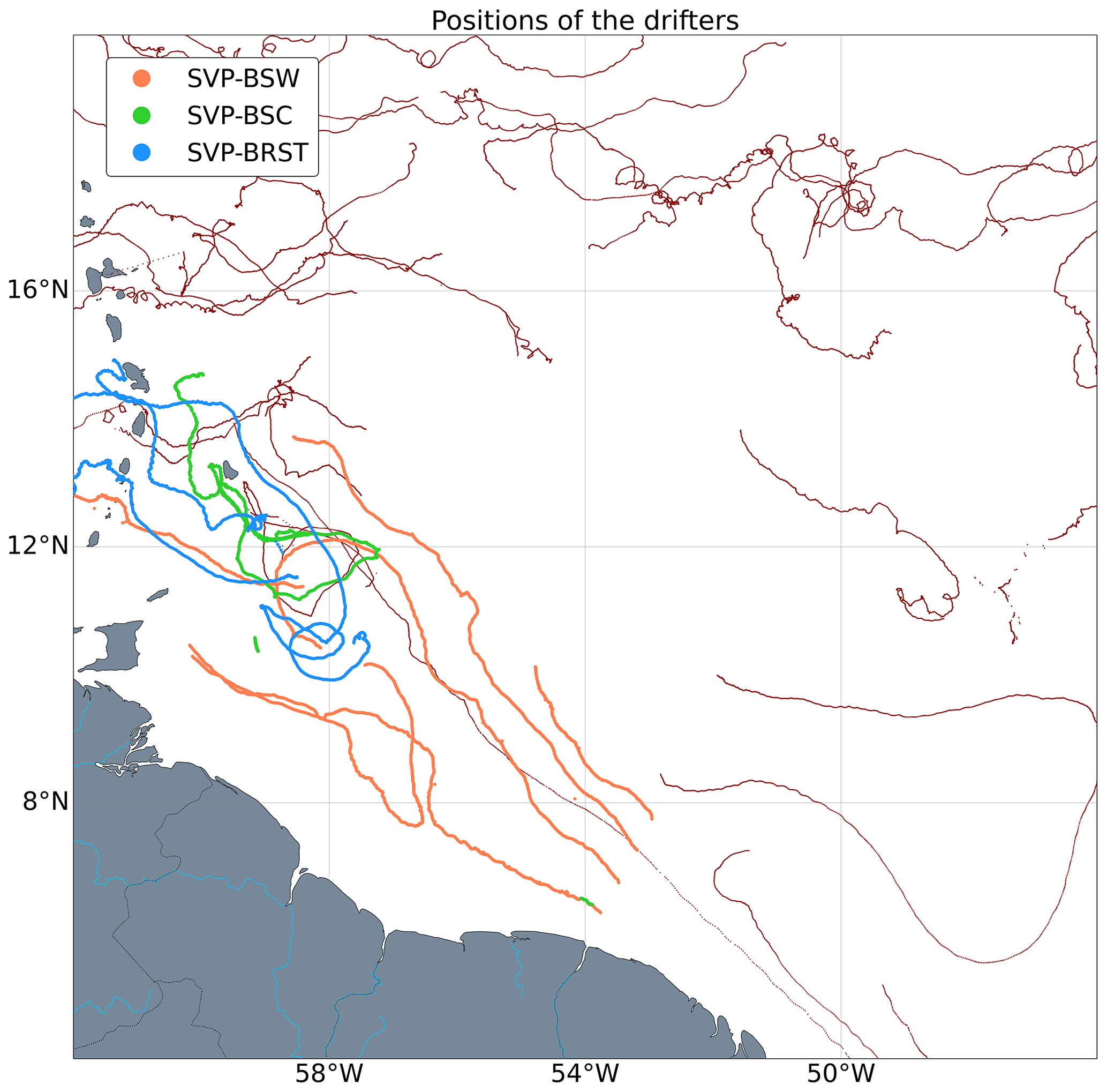
Figure 20 Map of the drifter positions from December 2019 to May 2020. Thick colored lines display the drifters that have been deployed from R/V L'Atalante, while thin red lines shows the other drifters observed in the region during the same period.

Figure 21 Panels (a), (b), and (c) show the absolute temperature differences between TSG/drifter pairs of measurements distributed in time and distance. Each pair is composed of one R/V's TSG measurement and a drifter's one. Respectively, panels (a), (b), and (c), correspond to the SVP-BSW, SVP-BSC, and SVP-BRST drifters. (d) Temperature differences as a function of time and distance for a pair of surface measurements. Differences are shown in blue for pairs of CTD-only profiles, in red for pairs composed of one TSG and one SVP-BSW measurement, in green for pairs composed of one TSG and one SVP-BSC measurement, and in purple for pairs composed of one TSG and one SVP-BRST measurement. Panels (e) to (g) are the same as above line for absolute salinity differences without the SVP-BRST drifters.

As Fig. 19 underlines, direct comparisons between Argo floats and nearby CTD stations are limited because of the low number of measurements. Moreover, since the float trajectories differ highly from that of the ship, the background oceanic variability estimated from the CTD might differ. Nevertheless, for nearby pairs of Argo and CTD profiles, the difference remains small. For ARGO floats and CTD stations found within 25 km, with five pairs of CTD/Argo profiles, the uncertainties for temperature and salinity are of $\mathrm{4}\times {\mathrm{10}}^{-\mathrm{2}}$ ^∘C and $\mathrm{1.5}\times {\mathrm{10}}^{-\mathrm{2}}$ psu. These uncertainties are of the same order of magnitude as those quantified for the other level 3 devices sampling the water column (uCTD and MVP).

Additionally, an optode sensor (for dissolved oxygen) from Aanderaa, with an accuracy of 4 µmol kg⁻¹, was mounted on the Argo floats deployed from R/V L'Atalante. In the same spatial and temporal range as the CTD stations, the dissolved oxygen sensors exhibit an uncertainty of 10 µmol kg⁻¹ for a 25 km range (see Fig. 19f).

4.4 Surface drifters

Four kinds of surface drifters were deployed from R/V L'Atalante during the experiment. Two Surpact drifters were launched for short periods of time, less than 2 d, and we will not describe them in detail here. Five SVP-BRST (Surface Velocity Program drifter with Barometer and Reference Sensor for Temperature) drifters from EUMETSAT (grant no. TRUSTED to Météo-France/CLS) measured temperature at 0.15 m depth, with an accuracy of $\pm \mathrm{5}\times {\mathrm{10}}^{-\mathrm{3}}$ ^∘C. Two SVP-BSC (Surface Velocity Program with Barometer–Salinity–Conductivity) drifters from Météo-France/L'océan (L'océan au cœur du système climatique) with CNES Soil Moisture and Ocean Salinity (SMOS) support measured temperature and salinity at 0.2 m depth, with a respective accuracy of ±0.1 ^∘C and $\pm \mathrm{5}\times {\mathrm{10}}^{-\mathrm{2}}$ psu, and were configured to send data every 6 min, with a sampling rate of 20 s. Finally, 10 SVP-BSW (Surface Velocity Program with Barometer–Salinity–Wind) drifters from NOAA were deployed to measure temperature and salinity, at 0.5, 5, and 10 m depth, with the same accuracy as SVP-BSC drifters and transmitting data every 30 min. Figure 20 shows the positions of these drifters, which exhibit clear advection toward the northwest, with some of them looping inside mesoscale eddies.

From R/V L'Atalante, two SVP-BSC and Surpact devices were deployed for short periods of time to compare their measurements with the similar devices and nearby instruments (Reverdin et al., 2021). Figure 21, similar to that for Saildrones, shows the comparison between surface TSG measurements and nearby drifter records. As for the Saildrones, these comparisons are delicate because the drifters measured temperature and salinity at different vertical levels near the surface, capturing a noticeably different background variability. The observed difference for the SVP-BSW drifters remains small for nearby pairs of measurements (less than 5 km apart and more than 300 pairs of measurements), with an uncertainty of $\mathrm{2.5}\times {\mathrm{10}}^{-\mathrm{2}}$ ^∘C for temperature and $\mathrm{2.5}\times {\mathrm{10}}^{-\mathrm{2}}$ psu for salinity. The SVP-BSC drifters' measurements exhibit a large difference in both temperature and salinity, $\mathrm{4.5}\times {\mathrm{10}}^{-\mathrm{2}}$ ^∘C and $\mathrm{2}\times {\mathrm{10}}^{-\mathrm{1}}$ psu, with more than 250 pairs of measurements found within 5 km. These large differences are particularly linked to one drifter. This is related to a large thermal effect upon deployment, supposedly becoming nearly negligible after a few hours. The manufacturer states that we should not consider the first few hours of data. Finally, temperature measurements from the SVP-BRST drifters follow the uncertainty from the TSG only, with an offset of about $\mathrm{2}\times {\mathrm{10}}^{-\mathrm{2}}$ ^∘C for 17 pairs of measurements found within 5 km.

5 Data concatenation

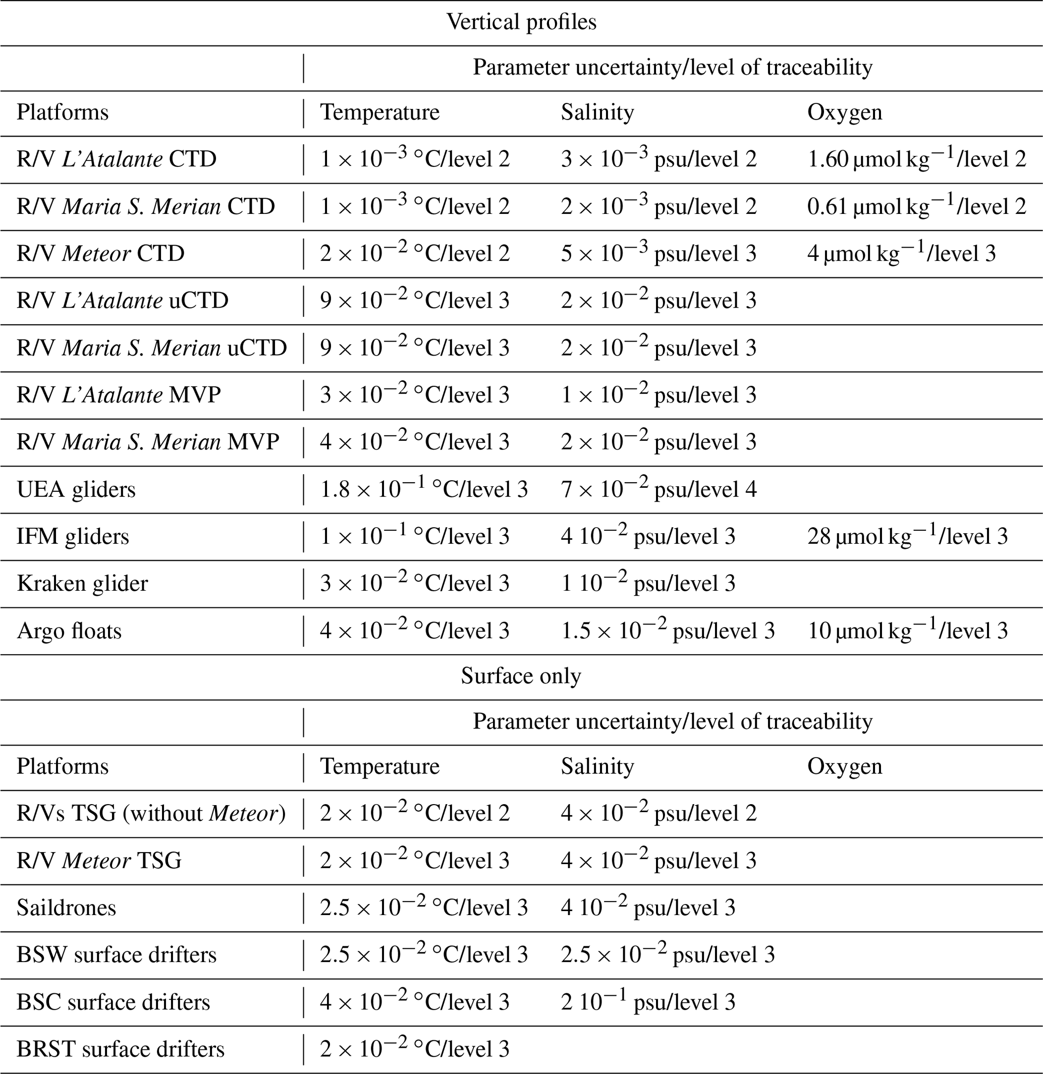
All the measured and cross-validated parameters can be associated with a level of uncertainty while using a concatenated dataset. Table 1 summarizes all the uncertainties calculated in this study. For example, for a vertical section of salinity from R/V L'Atalante, using CTD, uCTD, and MVP measurements, the associated uncertainties are $\mathrm{3}\times {\mathrm{10}}^{-\mathrm{3}}$ psu for the CTD, $\mathrm{2}\times {\mathrm{10}}^{-\mathrm{2}}$ psu for the uCTD, and $\mathrm{1}\times {\mathrm{10}}^{-\mathrm{2}}$ psu for the MVP. Thus, the dataset provides an array with different uncertainties for each type of profile.

Table 1 Table summarizing the uncertainties for each parameter measured by type of observation platform.

The concatenated data are very useful for enhancing the space–time resolution of many of the sampled areas and for better assessing the dynamical properties of the regional ocean circulation. With these data, it is, for example, possible to assess the relevant properties of surface and subsurface mesoscale eddies, freshwater filaments, cold water pools, and freshwater-induced barrier layers. Figure 22 shows the impact of the calibration on a specific section performed by R/V L'Atalante using CTD, uCTD, and MVP measurements. The first column, displaying only the CTD profiles, has a coarse horizontal resolution but is associated with low uncertainty linked to the validation and calibration processes. The second column presents the complete section, with the uncalibrated MVP and uCTD profiles. There we observe an increase in the horizontal resolution but nevertheless find some inconsistencies, as seen in Fig. 22b and c, with large variations between two successive profiles of salinity and potential density. Finally, after calibration, as seen in the last column, the uCTD and MVP profiles are corrected and cross-validated with the CTD measurements. The inconsistencies are removed while still keeping a high horizontal resolution and low uncertainty, enabling the calculation of realistic gradients of the different fields and the analyses of derived parameters, such as Ertel's potential vorticity (see Fig. 22e).

Figure 22 Vertical sections of thermohaline and dynamic characteristics performed by R/V L'Atalante. The first column shows the section with only the CTD profiles. In the second column the uncalibrated profiles of MVP and uCTD are added. The third column is the same but for calibrated profiles. Panel (a) is for temperature, panel (b) for salinity, panel (c) for potential density, panel (d) for oxygen (only CTD profiles measured oxygen), and panel (e) for Ertel's potential vorticity based on the ADCP measurements (not shown).

(Speich et al., 2021a)(Karstensen and Krahmann, 2023b)(Karstensen and Krahmann, 2023a)(Stevens et al., 2021)(L'Hégaret et al., 2020c)(Karstensen and Krahmann, 2023d)(L'Hégaret et al., 2020b)(Karstensen and Krahmann, 2023c)(L'Hégaret et al., 2020a)(Rollo, 2021)(Stevens et al., 2021)(Argo, 2000)(Stevens et al., 2021)(Karstensen et al., 2022)(Mohr et al., 2022)(Saildrone, 2020)(Stevens et al., 2021)

Table 2 Table summarizing the DOIs and parameters measured by type of observation platform.

6 Data availability

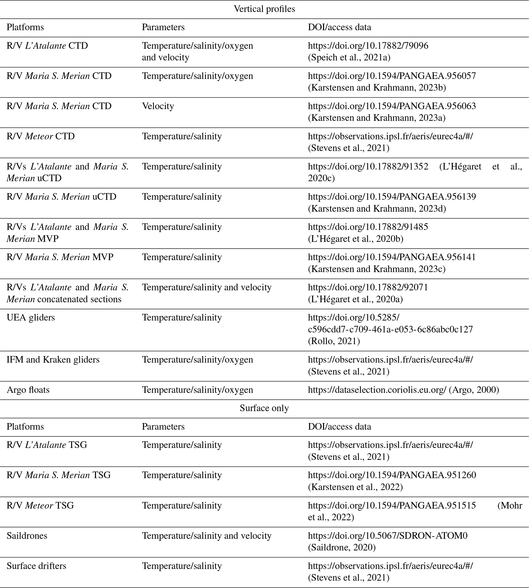
The underlying primary CTD and TSG datasets (in addition to the S-ADCP acquisitions) used in this study for comparison with other devices are available for each R/V on the AERIS website (https://observations.ipsl.fr/aeris/eurec4a/#/; Stevens et al., 2021). Additionally, for R/V L'Atalante, the CTD measurements can be retrieved from the SEA scieNtific Open data Edition (SEANOE) website (https://doi.org/10.17882/79096; Speich et al., 2021b, a). For R/V Maria S. Merian, the CTD thermohaline measurements are referenced on the Pangaea website (https://doi.org/10.1594/PANGAEA.956057; Karstensen and Krahmann, 2023b). The L-ADCP measurements, mounted on the CTD rosette from R/V Maria S. Merian, can be retrieved at https://doi.org/10.1594/PANGAEA.956063 (Karstensen and Krahmann, 2023a). Calibrated TSG measurements for R/Vs Maria S. Merian and Meteor are also available on the Pangaea website under the cruise names of MSM89 and M161 (https://doi.org/10.1594/PANGAEA.951515; Mohr et al., 2022), respectively (Karstensen et al., 2020; Mohr et al., 2020).

After the secondary data quality control process was applied, the various datasets were interpolated to the same vertical pressure grid with a 0.5 dbar resolution. This was done for temperature, salinity, and dissolved oxygen data and, when available, horizontal ocean currents. For each device, a NetCDF file is available for download on the SEANOE website, organized by type of device and ship, with its own DOI. The naming of the variables and parameters follows the convention of the NetCDF Climate and Forecast (CF) Metadata Conventions in Eaton et al. (2003). The secondary quality control uCTD and MVP profiles can be found on the SEANOE website (https://doi.org/10.17882/91352, L'Hégaret et al., 2020c; https://doi.org/10.17882/91485, L'Hégaret et al., 2020b). The original calibrated profiles from R/V Maria S. Merian are also available on the Pangaea website for the uCTD (https://doi.org/10.1594/PANGAEA.956139; Karstensen and Krahmann, 2023d) and for the MVP (https://doi.org/10.1594/PANGAEA.956141; Karstensen and Krahmann, 2023c).

Additionally, the concatenated sections described in the previous section, composed of CTD, secondary quality control uCTD and MVP profiles, and S-ADCP measurements from R/Vs L'Atalante and Maria S. Merian, can be accessed on the SEANOE website (https://doi.org/10.17882/92071; L'Hégaret et al., 2020a).

Measurements from the autonomous devices, Saildrones, underwater gliders, and drifters can also be retrieved from the AERIS website (https://observations.ipsl.fr/aeris/eurec4a/#/; Stevens et al., 2021). Furthermore, the UEA glider measurements are available on the British Oceanographic Data Center website (https://doi.org/10.5285/c596cdd7-c709-461a-e053-6c86abc0c127; Rollo, 2021). The NASA Saildrones can be access from the dedicated website (https://doi.org/10.5067/SDRON-ATOM0; Saildrone, 2020). Data from the Argo floats are available on the Coriolis website (https://dataselection.coriolis.eu.org/ and https://doi.org/10.17882/42182; Argo, 2000). Table 2 summarizes the different links and DOIs for accessing these various datasets.

7 Conclusions

The oceanic instruments deployed during the EUREC⁴A-OA experiment provide a large set of observations characterized by different oceanic structures, including mesoscale eddies intensified at the surface or at depth, finer-scale filaments, and salinity barrier layers. Nevertheless, the wide variety of devices at our disposal require precise pre- and post-cruise calibrations and cross-validations so that the data can be used to their full potential. In this study, we aimed to describe all sensors and their measurements, the sources of errors, and the methods used to correct them. Then, we ranked them, taking into account how they were validated and how they can be related to one another. The adopted strategy and the complementarity of the different observations enable the descriptions and quantification of such processes with unprecedented detail. This underlines the importance of deploying CTD stations and discussing their calibrations, which is our only way of comparing water parcels sampled at depth with sensor measurements by performing close-by profiles with other devices or attaching probes to the rosettes. Thereby, we are able to, at best, correct the measurements from other sensors or, at the very least, quantify their uncertainties.

Here we propose a way of estimating the uncertainties by assessing the three main sources of variability between measurements on isopycnal levels or at the surface, i.e., background oceanic variability (lateral variability and internal wave field) and the sensor variability. The background oceanic variability is highly depth dependent; thus, for comparison, we chose to compare profiles on isopycnal levels and only focus on measurements performed below the mixing layer. Nevertheless, this method largely depends on the number of observations and their calibrations and validations using water samples. It also underlines the importance of having synoptic profiles of the devices for comparison and, hence, corrections. In the end, we make a finalized dataset with calibrated and cross-validated thermohaline, chemical, and dynamical measurements available, together with their associated uncertainties after secondary QC.