the Creative Commons Attribution 4.0 License.
the Creative Commons Attribution 4.0 License.
 | 02 Dec 2022
Tropospheric water vapor: a comprehensive high-resolution data collection for the transnational Upper Rhine Graben region
Andreas Wagner
Bettina Kamm
Endrit Shehaj
Andreas Schenk
Peng Yuan
Alain Geiger
Gregor Moeller
Bernhard Heck
Stefan Hinz
Hansjörg Kutterer
Harald Kunstmann
Tropospheric water vapor is one of the most important trace gases of the Earth's climate system, and its temporal and spatial distribution is critical for the genesis of clouds and precipitation. Due to the pronounced dynamics of the atmosphere and the nonlinear relation of air temperature and saturated vapor pressure, it is highly variable, which hampers the development of high-resolution and three-dimensional maps of regional extent. With their complementary high temporal and spatial resolutions, Global Navigation Satellite Systems (GNSS) meteorology and Interferometric Synthetic Aperture Radar (InSAR) satellite remote sensing represent a significant alternative to generally sparsely distributed radio sounding observations. In addition, data fusion with collocation and tomographical methods enables the construction of detailed maps in either two or three dimensions. Finally, by assimilation of these observation-derived datasets with dynamical regional atmospheric models, tropospheric water vapor fields can be determined with high spatial and continuous temporal resolution. In the following, a collection of basic and processed datasets, obtained with the above-listed methods, is presented that describes the state and course of atmospheric water vapor for the extent of the GNSS Upper Rhine Graben Network (GURN) region. The dataset contains hourly 2D fields of integrated water vapor (IWV) and 3D fields of water vapor density (WVD) for four multi-week, variable season periods between April 2016 and October 2018 at a spatial resolution of (2.1 km)2. Zenith total delay (ZTD) from GNSS and collocation and refractivities are provided as intermediate products. InSAR (Sentinel-1A/B)-derived double differential slant total delay phases (ddSTDPs) and GNSS-based ZTDs are available for March 2015 to July 2019. The validation of data assimilation with five independent GNSS stations for IWV shows improving Kling–Gupta efficiency (KGE) scores for all seasons, most notably for summer, with collocation data assimilation (KGE = 0.92) versus the open-cycle simulation (KGE = 0.69). The full dataset can be obtained from https://doi.org/10.1594/PANGAEA.936447 (Fersch et al., 2021).
- Article
(2867 KB) - Full-text XML
-
Supplement
(1119 KB) - BibTeX
- EndNote


The atmosphere of the Earth contains only up to 4 % water vapor by volume or 25 mm global mean water equivalent. Still, atmospheric vapor is a highly effective greenhouse gas that is directly intertwined with global climate change (Stevens and Bony, 2013) and its implications for natural disasters such as floods, droughts, deluge, or glacier melting. As a vital component of the hydrological cycle, water vapor represents a major driver for the generation and spatiotemporal distribution of clouds and precipitation. Vertically integrated water vapor exhibits high variability of up to 0.5 mm within a range of a few kilometers and sub-hourly intervals (Vogelmann et al., 2015; Steinke et al., 2015). The continuous, extensive quantification of water vapor remains a challenge; while regional atmospheric models enable the simulation of the distribution of hydrometeorological variables in space and time at high resolution (Steinke et al., 2019; Giorgi, 2019), their skill is often limited by insufficient initial conditions or inadequate parameterizations of subgrid processes (Prein et al., 2015).
Water vapor is principally regarded as a source of noise in geodesy and remote sensing applications. The humidity of the Earth's atmosphere induces delays and distortions of high temporal and spatial fluctuations in microwave signals which cannot be eliminated by multi-frequency measurements and have to be quantified during the data processing. Thus, observations of Global Navigation Satellite Systems (GNSS) and Interferometric Synthetic Aperture Radar (InSAR) provide valuable contributions (GNSS has high temporal resolution; InSAR has high spatial resolution) for reconstructing the integrated water vapor (IWV) along the path from the satellites to the observation site on the Earth's surface (Bevis et al., 1992; Hanssen, 2001). Interpolation and approximation techniques like, for example, least-squares collocation or kriging, enable a sophisticated fusion of GNSS and InSAR products. In addition, the tomography-based evaluation of these data even allows the generation of three-dimensional fields of the water vapor distribution in space and time. Combining high temporal GNSS measurements with satellite products with low temporal but high spatial resolutions is obvious. Furumoto et al. (2003) applied GNSS water vapor measurements with radio acoustic soundings to improve water vapor profiles. Lindenbergh et al. (2008) combined Medium Resolution Imaging Spectrometer (MERIS) satellite data with GNSS data based on kriging techniques, and Leontiev and Reuveni (2018) used cloud fractions derived from Meteosat-10 to improve the GNSS IWV interpolation. The assimilation of GNSS measurements in atmospheric models to reduce uncertainties in water vapor simulations is another promising approach which is widely used (see Wagner et al., 2022, for a compilation), and the assimilation of InSAR-derived water vapor data can also improve the spatial skill of precipitation forecasts (Mateus et al., 2021). Although the combination of individual observational product types with atmospheric modeling is common, the rigorous fusion of multiple data sources with the latter has not, to our knowledge, been documented so far.
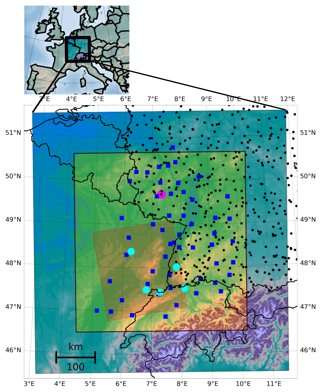
Figure 1Study area location and extent. Weather Research and Forecasting (WRF) model domain (650 × 670 km) and evaluation area (440 × 460 km; green area) with 56 GNSS stations for assimilation and tomography (blue squares), five GNSS stations for validation (cyan), 245 synoptic stations (black points), and the radiosonde station Idar-Oberstein (magenta). The red InSAR domain marks the core region where all datasets are available.
Therefore, we present here the interdisciplinary, high-resolution dataset of Fersch et al. (2021) of tropospheric water vapor and associated variables that incorporates all of the abovementioned methods, i.e., GNSS, InSAR, and regional atmospheric modeling, to provide a best guess of tropospheric water vapor for the transborder Upper Rhine Graben region of Germany, Switzerland, and France, where an extensive GNSS observation network is located (Fig. 1). We aim at combining the advantages of the respective methods and approaches, comparing the respective results, and creating new and improved datasets. In order to highlight the advantages and drawbacks of each approach and to elucidate the importance of comparing and combining different methods and disciplines, a brief introduction about methods and terminologies used by the different disciplines is provided in Sect. 2. Section 3 describes in detail the dataset and its creation process. Subsequently, we evaluate the dataset with independent observations in Sect. 4. The abbreviations and acronyms used in the text are summarized in Table B in the Appendix.
As tropospheric water vapor concentrations are highly changeable with space and time, the techniques for their assessment likewise need to be precise. The common observational methods are usually good in certain aspects but also come with crucial drawbacks. Radiosounding with balloon sondes, for example, provides measurements of pressure, temperature, wind, and humidity at high vertical resolution. However, due to the effort of assembling the device and because of the sparse density of release stations, the spatial distribution of such measurements allows only for local or large-scale applications, such as airfield control or numerical weather prediction. Other methods like, for example, satellite remote sensing, allow for higher spatial resolution but at the cost of vertical integration or reduced temporal resolution. Obviously, the combination of different observation methods depicts a way to overcome the limitations of the individual techniques. Similarly, with data assimilation, dynamical atmospheric downscaling can provide a best guess of the tropospheric water vapor with high temporal and spatial resolution.
In the following, and also to make readers familiar with the terminologies used by the different disciplines, we provide a brief overview of the respective methods for tropospheric water vapor observation and modeling and also highlight how the strengths of the different data sources can be combined into something more valuable.
2.1 Observation
2.1.1 Local profiles
Local profiles of tropospheric water vapor conditions can be obtained with radiosondes, ground-based radiometry, or laser techniques. According to Rocken et al. (2004), the global radiosonde network has about 850 stations with at least two releases per day. With inter-station displacements of several hundreds of kilometers, the measurements do not qualify for the determination of local high-resolution tropospheric water vapor fields but are valuable for the validation of other observation techniques (e.g., Divakarla et al., 2006; Reale et al., 2008; Jin et al., 2011) or can be used in combination with satellite observations on the global scale (e.g., Randel et al., 1996; Shi et al., 2016). Ground-based microwave radiometers and infrared spectrometers provide tropospheric profiles of temperature and humidity for direct and slanted paths but require the application of complex retrieval algorithms. According to Löhnert et al. (2009), accuracies for humidity can be as good as 0.25–0.5 g m−3 during clear-sky conditions, but the method is limited if clouds are present. For complex terrain, Massaro et al. (2015) found that, within the boundary layer, detailed humidity profiles cannot be derived. Nevertheless, with accuracies below 1 kg m−2, the method is well suited for vertical integrals of water vapor (Almansa et al., 2020), but the measurements are mostly restricted to the lower troposphere (Feltz et al., 2003; Pospichal and Crewell, 2007; Fersch et al., 2020). The light detection and ranging (lidar) method (e.g., Klanner et al., 2021) is a further way to obtain high-resolution water vapor profiles with high accuracies. The complexity of ground-based radiometers and lidar systems has so far prevented the realization of such kinds of networks, meaning that no observations of tropospheric water vapor profiles are available at the kilometer to sub-kilometer resolution.
2.1.2 GNSS-derived tropospheric variables
The ground-based Global Navigation Satellite Systems (GNSS) technique for the monitoring of atmospheric water vapor was implemented in the early 1990s (Bevis et al., 1992). The GNSS signals received at the Earth's surface are delayed by atmospheric refraction. The delay depends on the atmospheric state and can be transformed with mapping functions, from slant to vertical paths, so that zenith total delay (ZTD) is obtained. ZTD can be decomposed into zenith hydrostatic (or dry) delay (ZHD) and zenith wet delay (ZWD). ZHD can be precisely modeled with the measured surface pressure Ps (Saastamoinen, 1972; Davis et al., 1985). ZWD is the difference in ZTD and ZHD, and because of its relation with atmospheric water vapor, it can be converted to IWV by utilizing the atmospheric weighted mean temperature Tm (Bevis et al., 1994).
With tens of thousands of stations worldwide, the ground-based GNSS technique provides valuable information about the water vapor variability. With key advantages of all-weather operability, high accuracy, high temporal resolution, and wide distribution over land (Jones et al., 2019), GNSS tropospheric estimates became an important data source for meteorological and climatological applications. For example, they are being used to observe the water vapor variability during extreme weather events (e.g., Zhu et al., 2020). In addition, long-term time series of IWV derived by ground-based GNSS contain valuable information about the water vapor feedback effect due to climate change (e.g., Alshawaf et al., 2018; Yuan et al., 2021).
The accuracy of the IWV retrievals is limited by the uncertainty in the ZTD estimates in addition to the availability and quality of Ps and Tm observations at the GNSS stations. Ideally, Ps and Tm can be accurately measured by synoptic barometers and co-located radiosondes, respectively. In this case, the uncertainty in GNSS-derived IWV can reach 0.6 kg m−2 (Ning et al., 2016). However, not every GNSS station is equipped with a barometer, and only few stations are co-located with radiosondes. Hence, accurate Ps and Tm obtained from atmospheric reanalyses or numerical weather predictions (NWPs) have been used in the retrieval of GNSS IWV (e.g., Wang et al., 2005).
2.1.3 InSAR-derived tropospheric variables
Similar to the propagation delay measured with GNSS, the radar signal of the Synthetic Aperture Radar (SAR) satellites experiences a phase delay due to water vapor in the atmosphere (Hanssen, 2001, chap. 3.4). Interferometric analysis of two or more SAR acquisitions of the same area reveals the difference in the integrated phase delay between these acquisition times along the SAR line of sight (LOS), i.e., along the travel path between the sensor and the observation point on the ground (Heublein, 2019).
SAR satellites are usually deployed at sun-synchronous low Earth orbits. SAR instruments are side-looking, imaging in a slanted direction, with usual incidence angles between 18–50∘. The integrated delays are therefore observed along a slant ray, corresponding to the LOS. A main issue with using InSAR data over long periods is the decorrelation of the signal as soon as the backscatter characteristics of the ground begin to change over time. Therefore, only long-term stable points, so-called persistent scatterers (PSs) are used (Hooper et al., 2007; Ferretti et al., 2001). Naturally, PS points are irregularly distributed with high PS density in urban areas and sparse PS occurrence in rural and vegetated areas.
Whereas the benefit of InSAR-derived zenith delays is the high spatial resolution, large-scale regional trends, and the absolute datum is less reliable and prone to errors due to the differential nature of the interferometric measurement but also due to additional signal components like crustal tides, tidal loading, and residual orbital errors which cause long wavelength signals. Thus, further knowledge or external data need to be introduced as an additional constraint to solve the datum defect and adjust spatial trends, i.e., the signal component with long wavelengths of the estimated IWV.
2.2 Numerical atmospheric modeling and data assimilation
The performance of numerical weather prediction (NWP) and climate models typically goes in line with the accuracy of the simulated tropospheric and, in particular, the planetary boundary layer (PBL) water vapor fields (Gallus and Segal, 2001; Jochum et al., 2004; Kunz et al., 2014; Jiang et al., 2020). All of the global circulation models that are employed for operational forecasting or retrospective analyses (reanalyses), ingest vast numbers of atmospheric water vapor observations, mostly based on satellite remote sensing. The benefits of this practice are well proven, e.g., for the Integrated Forecasting System (IFS) of the European Centre for Medium-Range Weather Forecasts (ECMWF; Andersson et al., 2007) or the ERA-Interim reanalysis of ECMWF (Dee et al., 2011). While the global operational NWPs develop towards convection-resolving resolutions, ∼ 13 km for the Global Forecast System (GFS; Zhou et al., 2019) and ∼ 9 km for ECMWF's IFS, the global reanalyses stay a bit behind, with resolutions of up to ∼ 30 km for ECMWF's ERA5. A further increase in the spatial resolution can be achieved with limited area models (LAMs) that perform a downscaling for subregions of the global models. Typically, LAMs exhibit more detailed process descriptions as, for example, with a non-hydrostatic formulation of vertical motion, the consideration of air compressibility, or acoustic gravity waves. The quantitative performance of the LAMs depends on the quality of initial state and on time-varying boundary conditions.
The incorporation of additional water vapor information, even on a smaller scale, is possible through data assimilation. The positive impact of the assimilation of InSAR data (Pichelli et al., 2015; Mateus et al., 2016, 2021) and GNSS stations (Pondeca and Zou, 2001; Poli et al., 2008; Boniface et al., 2009; González et al., 2013; Lindskog et al., 2017; Giannaros et al., 2020) is shown for numerous studies and regions. Variational data assimilation schemes merge atmospheric models and observations while considering their respective error statistics by iteratively minimizing a cost function. For further information, we refer the reader to Ide et al. (1999), Barker et al. (2003), and Barker et al. (2004).
2.3 Data fusion
Each of the above-discussed techniques for atmospheric water vapor estimation has specific strengths and weaknesses. The fusion of different data products and modeling approaches allows the exploitation of the complementing characteristics so that the tropospheric water vapor estimation becomes more accurate, reliable, and robust.
2.3.1 Fusion of GNSS and InSAR
Although the atmosphere affects GNSS and InSAR similarly, their tropospheric products have differing characteristics, mostly because of their different geometric settings and due to the fact that GNSS relies on sparse, though highly precise, 3D point determination on the ground, while persistent scatterers interferometry (PSI) relies on opportunistic, appearance-based, but less accurate, point scatterer detection. On the one hand, the most typical GNSS tropospheric product is the ZTD, an absolute measurement (at meter level) which represents the integral of the refractivity in the zenith direction and is provided at centimeter-level accuracy nowadays (Teunissen and Montenbruck, 2017). The ZTDs are provided with a high temporal resolution, such as hourly or even every 5 min. However, the spatial resolution is relatively low, depending on the density of GNSS networks. On the other hand, InSAR-retrieved atmospheric maps consist of relative tropospheric delays (at centimeter level) obtained at very low temporal resolution (days, weeks, or even months) but with a very high spatial density up to meter level. In this paper, we aim to exploit the synergies of both techniques, by combining their tropospheric delays, to retrieve enhanced water-vapor-related products (delays or refractivities). For this purpose, we fuse GNSS ZTDs with InSAR differential slant total delays (ddSTDs) in the least-squares collocation software COMEDIE (Collocation of Meteorological Data for Interpretation and Estimation of Tropospheric Path Delays; Eckert et al., 1992a, b), which is upgraded to process the measurements from the different techniques simultaneously. Shehaj et al. (2020) describes the framework to combine GNSS and InSAR tropospheric delays, with the goal of retrieving tropospheric delays at any point of an investigated area. The same principles of combination are applied to the dataset discussed in this paper.
2.3.2 Tomography
GNSS tomography allows for the distribution of the water vapor content to be resolved in 4D (space and time); thus, the height profiles of the water vapor can be determined (Moeller, 2017). The basis of most tomography software packages are slant path delays. In tomography, the atmosphere in the investigated area around the GNSS network is discretized in a 3D voxel model. By exploiting the relation between the slant delays and the geometric ray paths, refractivity N in each of the atmospheric voxels is obtained.
In this work, an alternative tomography approach is suggested, based on the collocation of ZTDs and STDs using software COMEDIE. The functional and stochastic models for retrieving the refractivity are obtained by forming the derivatives of the ZTD model with respect to height, as detailed in Sect. 3.5 and Hurter (2014). When combining InSAR measurements with GNSS measurements to obtain refractivity fields, the stochastic models that connect the InSAR slant delays with the refractivity are simply the models relating the zenith delays with refractivity mapped in the slant direction; this is clear, since we treat the slant delays as mapped zenith delays in the slant direction (Shehaj et al., 2020).
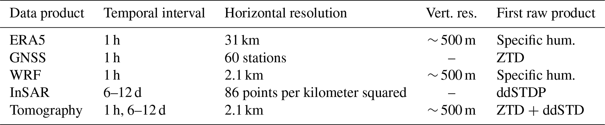
The dataset presented in this work was produced with the aim of providing the best possible assessment of regional, high-resolution tropospheric water vapor fields founded on established observation methods and data assimilation. For this purpose, we selected the area of the GNSS Upper Rhine Graben Network (GURN; Fig. 1), where GNSS, InSAR, and radiosonde observations are available. We derived data products from different combinations and fusions of the individual observations and by assimilation with the limited area Weather Research and Forecasting modeling system (WRF-ARW; Skamarock and Klemp, 2008). As illustrated in Fig. 2, the collection features IWV, ZTD, ZWD, water vapor density (WVD), and double differential slant total delays in phase values (ddSTDP), derived from GNSS, SAR, and atmospheric modeling techniques. The temporal and spatial features of the basic data products are listed in Table 1.
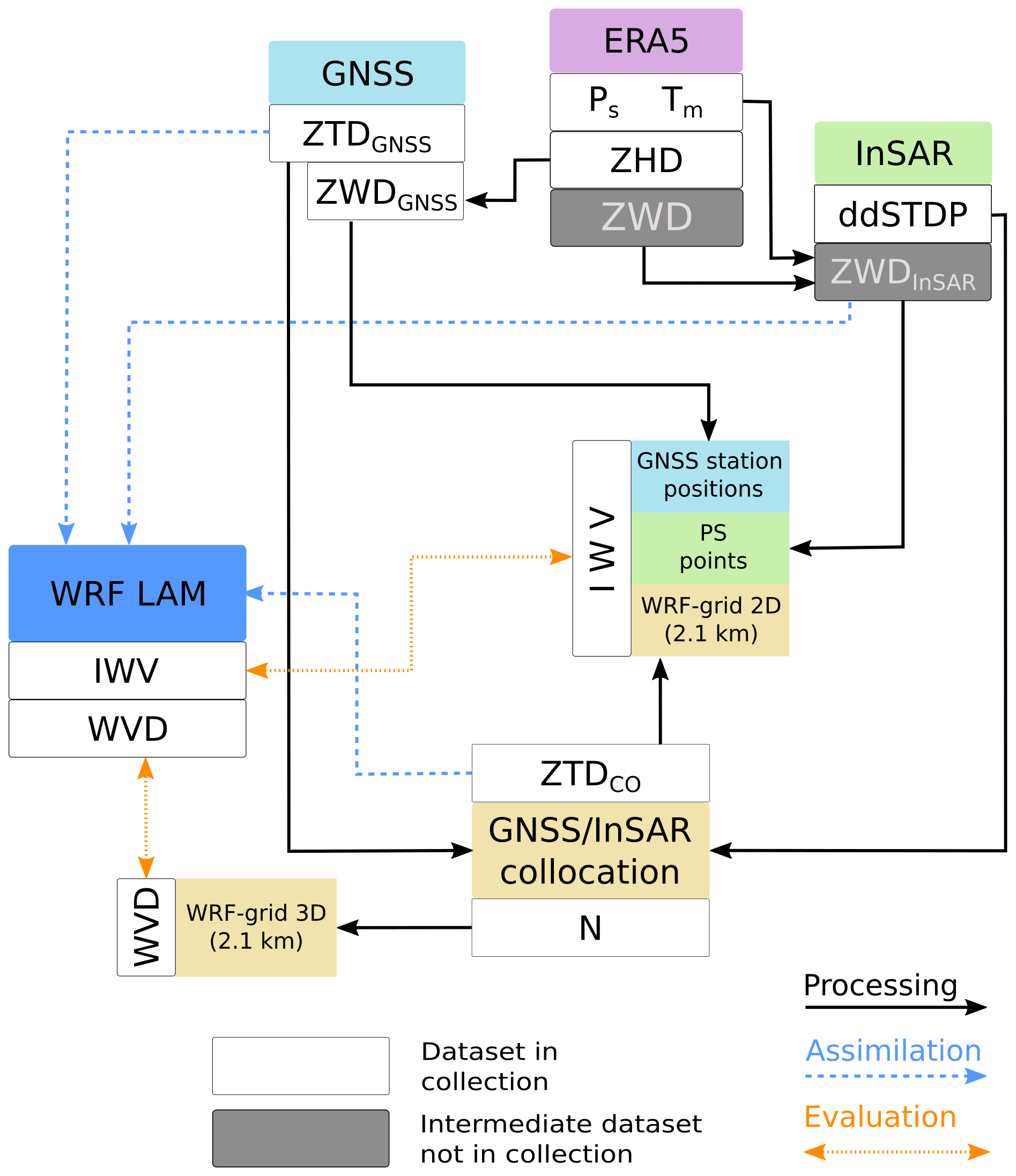
Figure 2Dataset overview sketch. The lines depict the following pathways: black (solid) – data processing; blue (dashed) – data assimilation; orange (dotted) – evaluation. The white fields denote the products contained in the data collection, and the gray fields mark intermediate (unpublished) data.
Table 1Temporal and spatial properties of the basic data products which were used to generate the combined dataset.
To cover the characteristic seasons of the Northern Hemisphere, we selected four investigation periods for which we processed all of the data products (11–22 April 2016, 13–24 July 2018, 16–31 October 2018, and 6–21 January 2017). Some of the individual datasets, i.e., the processed InSAR scenes and the GNSS ZTDs, extend beyond those preselected periods or the boundaries of the GURN study region. Our intention was to provide the data as comprehensively as possible to foster further scientific studies. For better comparability, the same variables were determined for all datasets, i.e., integrated water vapor (IWV) for 2D data and water vapor density (WVD) for 3D data. In addition, the ERA5 reanalysis is used for all conversions that require additional meteorological input such as pressure and temperature. Moreover, we document the full processing chain so that it can be reproduced by others or be repeatedly applied as more recent data or alternative products become available. In the following, we describe the characteristics of the study region and the methods that have been used to provide the individual and the combined data products.
3.1 Study region
The core region is defined by the transnational GURN that was originally established for the investigation of tectonic activities (Mayer et al., 2012). It encompasses the southwestern part of Germany and the eastern part of France, with the Upper Rhine Graben (URG) in the center, the Black Forest in the east, and the Vosges in the west, plus a small area of northwestern Switzerland (Fig. 1).
The Upper Rhine Valley is one of the warmest regions of Germany, with lower annual rain amounts (approx. 600 mm a−1) but with high convective activity in the summer months. Up to 1500 mm a−1 of annual rain amounts are measured in the low mountain ranges of the Black Forest, the Vosges, and the Swiss Jura and about 1000 mm a−1 in the flatter western and northwestern area.
3.2 GNSS-derived IWV and ZTD
The global positioning system (GPS) observations of 66 stations of the GURN were used to estimate IWV. GURN was established by the Geodetic Institute (GIK) of Karlsruhe Institute of Technology, Germany, and the École et Observatoire des Sciences de la Terre of the University of Strasbourg and the French National Center for Scientific Research. Currently, GURN consists of ground-based GNSS stations from permanent authoritative and private GNSS networks. In Germany, this refers to SAPOS (the German satellite positioning service operated and maintained by the mapping agencies of the German federal states) and GREF (Integrated Geodetic Reference Network of Germany; this is the responsibility of the Federal Agency for Cartography and Geodesy, BKG). In France, the respective networks (providers are given in parentheses) are RENAG (national GNSS network of French research laboratories; French National Centre for Scientific Research, CNRS), RGP (National Institute for Geographic and Forestry Information, IGN), and the GNSS networks of the providers TERIA and SATINFO. In Switzerland, data from the permanent GNSS network of the federal mapping agency swisstopo are used. Several stations from International GNSS Service (IGS) and EUREF are also included. For the availability of the raw GNSS observations, readers are referred to the data providers' specific policies. Up to now, only GPS observations have been processed. Other GNSS systems like GLONASS (Russian satellite navigation system) and Galileo will be added in the future.
The GPS data were processed with the GAMIT software (version 10.7; Herring et al., 2018) for all InSAR dates and for the four seasonal investigation periods. To model the tropospheric delays of GPS signals received by the ground-based stations, we adopted the following equation to map the slant signals into zenith:
with the corresponding mapping functions mfH and mfW. The term grad is a function to model the effects of azimuthal asymmetry in the tropospheric delays, where a and e are the azimuth and elevation angles of the GPS signals, respectively:
In this study, we used the a priori zenith hydrostatic delay from European Centre for Medium-Range Weather Forecasts (ECMWF; Simmons and Gibson, 2000), the state-of-the-art Vienna Mapping Functions 1 (VMF1; Boehm et al., 2006), provided by the Vienna University of Technology, and the tropospheric gradient model proposed by Chen and Herring (1997). Moreover, we also conducted the GPS data processing with other advanced strategies and models. For example, we removed the first-order effect of the ionospheric delay with linear combinations of observations and modeled its second- and third-order effects with International Geomagnetic Reference Field 12 (IGRF12; Thébault et al., 2015) and ionospheric data from the Center for Orbit Determination in Europe (CODE; Schaer, 1999). We removed the observations with elevation angles lower than 10∘ and weighted the other observations according to their elevation angle and their post-fit-phase residuals. We modeled and corrected solid Earth tides, ocean tides, and pole tides according to International Earth Rotation and Reference Systems Service (IERS) Conventions 2010 (Petit and Luzum, 2010). We used the IGS final orbits, IGS absolute-antenna-phase center models (Schmid et al., 2016), and ITRF2014 reference frame (Altamimi et al., 2016).
The tropospheric products derived by the GPS data processing include ZTD, gradients in the north/south and east/west directions, and their corresponding standard deviations, respectively. The ZTD estimates were further used for the retrieval of IWV, with auxiliary information (i.e., Ps and Tm) obtained from ERA5 pressure-level products. Detailed procedures for the IWV retrieval from ground-based GPS are provided in the Appendix A1.
The GPS tropospheric outputs for all the stations, auxiliary variables from ERA5, and the retrieved IWV are saved day by day in ASCII files in Solution (Software/Technique) INdependent EXchange Format for TROpospheric and meteorological parameters version 2.00 (SINEX_TRO V2.00). The SINEX_TRO V2.00 format was designed to accommodate related developments. For example, it supports tropospheric variables derived by numerical weather prediction models and reanalyses in addition to space geodetic techniques. The SINEX_TRO V2.00 file is composed of groups of data termed as blocks. Each block has a specific format. Some of the blocks are mandatory (e.g., reference block), whereas the others are optional (e.g., comment line). Thus, the structure of the SINEX_TRO V2.00 format is very simple and flexible. For the details on the definition of the SINEX_TRO V2.00 format, readers are referred to Pacione and Douša (2017).
The file names of the GPS tropospheric products are in the style of gikyrdoy0.txt, where gik is the name of the data provider, yr and doy are year in two characters and day of year in three characters, respectively. The files start with metadata blocks and end with data blocks. The metadata blocks include information on the data providers, data processing strategies and models, station names, coordinates, receiver types, antenna types and eccentricities, and so on. The data blocks list the GPS-derived ZTD, gradients, and their corresponding standard deviations, respectively. In addition, the data blocks also include the Ps, ZHD, and Tm from ERA5, as well as the final ZWD and IWV estimates.
3.3 InSAR-derived ddSTDP and IWV
To derive double differential slant total delays in phase values (ddSTDP) and IWV from PSI, we use Sentinel-1A/B data, acquired at an altitude of around 690 km in interferometric wide swath mode (IW), with a ground resolution of around 5 × 20 m and a swath width of 250 km. The data were recorded by both satellites (A and B) along ascending orbit 88 between March 2015 and July 2019. All available datasets are visualized over time and the along-track coverage in latitude is indicated in Fig. S4 in the Supplement. Each scene is displayed in a different color, with additional labels for the four study events. The satellite repeat cycle is 12 d, and combining data from both satellites has nominally provided an acquisition on every sixth day since the launch of Sentinel-1B in October 2016. The acquisition time, 17:26 UTC, is constant for both satellites. With the given repeat cycle of the two satellites, 213 scenes could be theoretically available. But some gaps occur in the dataset at certain time intervals, e.g., when the project area was not covered for different reasons, leading to the finally processed 169 scenes. In this study, we processed the VV (vertical transmit, vertical receive) polarized data and used the Shuttle Radar Topography Mission (SRTM) 1 as a reference digital elevation model during processing. The orbit correction was performed with the provided precise orbit files.
InSAR processing was performed using the software SNAP, starting with version 7.0, and from the coregistration step onward, version 8.0 was used (SNAP, 2021). For further PS processing, we then used the program StaMPS (version 4.1-beta; Hooper et al., 2012) for the PSI processing. The master scene for the interferometric processing is from 17 March 2017. The spatial reference point was chosen at the town of Épinal at (6.45066∘ E, 48.175043∘ N), with a reference radius of 1 km. As such, we obtain an intermediate dataset of raw double differential slant total delays (ddSTDP) for each interferogram and each PS, which is provided in the dataset publication in the common StaMPS format. Afterwards, we estimated the linear displacement at each PS point with a weighted ensemble estimation and removed the displacement phase from the observations. The resulting corrected partial differential slant-phase delays (pSWDs) are used for the tomographic approach. They are then mapped to zenith direction using the sine function, as follows:
with the looking angle ψ and the partial wet delays in the slant (pSWD) and zenith (pZWD) direction. Those corrected-phase observations in the zenith direction were then used as input to the Atmospheric Phase Screen (APS) inversion. It is based on the zero-mean assumption and is performed point-wise for each PS point independently. The zero-mean assumption does not consider the different heights of PS points. This results in a systematically different behavior of the different PS points due to the stratification of the water vapor in the atmosphere. Therefore, we refer to these values as partial zenith wet delays (pZWDs). The bias induced through the zero-mean assumption is corrected point-wise using reference values extracted from the ERA5 reanalysis (ECMWF, 2020) to ensure a datum adjustment to the true mean wet delay. The calculation of the required ZWD and mean temperature (Tm) was performed analogously to that described in the GNSS processing section (Sect. 3.2) and in Appendix A1.
PSI pZWD contains signal components with long wavelengths which can be biased for several reasons. Therefore, spatial trends over the whole imaged region were re-estimated in the next step. To include only the atmospheric signal, a quadratic function f(ϕ,λ), as in Eq. (6), was estimated, which describes the difference between pZWD derived from the ERA5 dataset and the PS–InSAR mean-corrected data. This function depends on geographic longitude λ and latitude ϕ. The estimation parameters , and e differ for each of the 169 scenes.
The optimal function is determined using a bootstrapping approach. This approach uses several small subsets of all available PS points to reliably calculate the optimal function (Efron, 1979). The ZWDs were then calculated using the optimal function to correct the mean-corrected ZWDs. Subsequently, the ZWDs were transformed to IWV according to Eq. (A4).
Finally, we derive the IWV for each PS point, which is corrected for height errors and includes long wavelength atmospheric signals. The precision of the IWV is estimated for a given PS point as standard deviation of all points located in a 200 m radius with regard to this point. The inner precision of the IWV dataset is 0.27 kg m−2, which is the average value over all PS points.
The two products provided in the data compilation, for all 169 dates and at each PS point location, are (1) the double differential slant total phase delays (ddSTDPs) and (2) the integrated water vapor (IWV). A potential application of these products is the improvement in methods for gridding and the calculation of APS to IWV. The second product can be used for assimilation purposes in weather models.
3.4 WRF-based dynamical downscaling and data assimilation for IWV and WVD
We applied the three-dimensional variational data assimilation (3D-Var) system provided by WRF (Barker et al., 2003, 2004) to assimilate IWV, WVD, and additional synoptic station data.
Convection permitting WRF simulations with hourly output were performed for each of the four seasonal study events on the basis of hourly ERA5 driving data (Hersbach et al., 2020). The choice of model physics (see Table 2) is widely adopted from another study in the same region by Wagner et al. (2018) and outlined in more detail in Wagner et al. (2022).
(Mlawer et al., 1997)(Dudhia, 1989)(Hong and Lim, 2006)(Hong et al., 2006)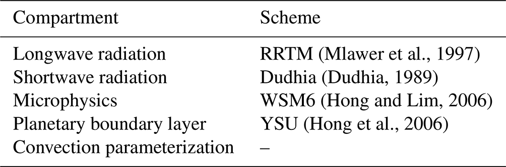
The domain encompasses an area of approximately 650 × 670 km, with a grid spacing of 2.1 km and 72 vertical levels (created automatically by the WRF). This domain size should guarantee spatial spinup. The temporal spinup is based on several weeks of open-cycle simulations before each event to achieve satisfying soil conditions. Open-cycle simulations are WRF simulations with hourly ERA5 input but no assimilation of additional variables. In this way, reliable starting conditions for the assimilation comparisons were obtained. We performed three simulation runs for each of our chosen events. Run1 is based on the assimilation of meteorological stations, GNSS and InSAR data. For Run2, meteorological station data and tomography data were used, and Run3 is an open-cycle simulation. The 3D-Var technique, which is implemented in the WRF Data Assimilation (WRFDA), was applied for the assimilation runs. The multivariate background error statistics option cv6 was chosen (Barker et al., 2004). In this way, temperature is also able to show a direct impact on moisture, and vice versa. A spatial thinning of 10 km was used to minimize correlation artifacts. To tie the simulations closer to the measurements, all assimilation input data, except InSAR data, were assimilated on an hourly basis. This is particularly useful when the variations in water vapor in the lower atmosphere are more complex due to dynamic weather conditions. Temperature, pressure, and relative humidity from meteorological stations were used, along with ZTDs from GNSS, InSAR, and interpolated fields, by means of collocation. The tomography data are based on the same GNSS data as in Run1 but offer gridded input on the WRF grid. The calculation of the ZTD values from GNSS stations and tomography is explained in the respective chapters. ZWD data were provided from InSAR measurements. The dry signal part (ZHD) was calculated from the respective WRF open-cycle simulation and was added to the InSAR ZWDs in order to achieve ZTD values for assimilation.
The applied solvers, model time steps, and other simulation parameters in WRF are defined in a table called namelist.input. This file is included in the dataset together with a netCDF file called geo_em.d01.nc. It contains all static fields in 2D or 3D for the WRF model in the chosen projection, such as altitude, land use, soil information, etc. Additionally, the background error covariance matrix (be.dat) is required for the assimilation. It was calculated with the NMC method (Parrish and Derber, 1992) for each of our events. Based on month-long WRF simulations with the same setup as our open-cycle simulations, averaged forecast differences in the 12 and 24 h forecast (valid at the same time) were applied. Furthermore, the assimilation input for Run1 is provided (obsproc_hour). This is a pre-processed input, where observation errors were included and duplicates and inconsistence data due to certain tests were removed. For raw assimilation data, we refer to the other datasets presented in this section. The meteorological station data are available at DWD (German Meteorological Service; DWD, 2020). The forcing data from ERA5 can be obtained from the ECMWF website (ECMWF, 2020).
WRF output is available on the 3D model grid. The direct nesting from 31 to 2.1 km reduces possible artifacts due to intermediate domains and the respective parametrizations (e.g., convection), on the one hand. On the other hand, model physics require a larger area to evolve. That is why we discarded an area of 50 pixels at the borders to achieve reliable simulation outcomes. The results are provided after 1 h of free WRF simulations to obtain consistent model data, since the assimilation of variables modifies only certain model variables. Temperature, pressure, and water volume density are provided on a 3D grid (219 × 209 × 72). In 2D, temperature and pressure are provided in 2 m, and integrated water vapor (IWV) and rain amounts are given as column values.
3.5 ZTD, refractivity, and WVD based on collocation
The least-squares collocation approach is based on a functional and a stochastic component, where correlated parts are determined and separated from uncorrelated measurement noise as follows (for instance, from Eckert et al., 1992a):
where l is the measurement, is the functional part representing realistic physical models of meteorological variables with u, x, and t, which are, respectively, the state vector to be estimated, the coordinates, and the time. The so-called signal depends on an empirically modeled covariance Css, and the noise ϵ is assumed to be stochastically uncorrelated.
In our collocation software, the state vector to be estimated is . ZTD0 is the ZTD at reference position , aZTD, bZTD, and cZTD are gradients in the x,y coordinates and time, and HZTD is the scale height. represent the coordinates and time of a measured point. MFs are mapping functions used to map zenith delays in the slant direction. Thus, according to Hurter (2014) and Shehaj et al. (2020), the ZTDs and ddSTDs (both in millimeters) are modeled as follows:
For the ddSTDs, the superscripts t1,tref represent the time of acquisition of an InSAR image and the reference image acquisition time, thus forming the time difference, while the subscripts p1,pref refer to the positions of an InSAR PS point in the image and the position of the reference PS point forming the spatial difference. The formulas describing the covariance of the signal part can be found in Eckert et al. (1992a) and Eckert et al. (1992b).
For the collocation of GNSS and InSAR measurements, the following two steps are required:
-
Screening of GNSS ZTDs and InSAR ddSTDs, based on a simple least-squares estimation and gross error detection. The value of the residuals divided by the product of the a posteriori standard deviation and measurement noise is compared to a preselected threshold.
-
Least-squares collocation of the measurements passing the screening process. The signal and the noise of each measurement are defined, respectively, by the covariance of the signal Css and the covariance of the noise (which is a diagonal matrix describing the variance of each measurement).
The refractivity (N, in parts per million) equals the derivative of the delay in the direction of the ray. Thus, by deriving the zenith delays with respect to height, we obtain the following:
The covariance matrices relating delays with refractivity, as shown in Hurter (2014), are obtained by deriving the covariance of the delays with respect to height.
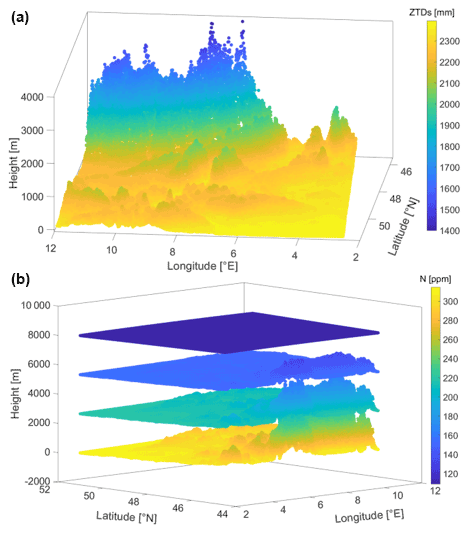
Two kind of products are provided in this study, namely (1) 2D maps of ZTDs interpolated onto the grid of the WRF domain (Sect. 3.4) which contain structural information of the lowest tropospheric layer and (2) 3D tomographic products in the form of refractivity fields on the horizontal grid of the WRF domain. For the vertical distribution, the refractivities are computed for 16 equally distributed layers, from the lowest WRF layer up to 8 km.
Examples of ZTDs and refractivity fields, obtained using our approach, are shown in Fig. 3 for the spring event of 2016. From the top plot in Fig. 3, it can be noticed that the ZTDs and the refractivity fields for the lowest layer follow the topography of the terrain, while, in the bottom plot, the decrease in refractivity with altitude is visible.
A further, extended, time series of tomographic products is provided based on the InSAR and GNSS collocated tropospheric products, as described in Sect. 3.2 and 3.3. The length of the time series corresponds to the number of InSAR acquisitions, since the scope is to exploit the two techniques simultaneously. Therefore, the temporal resolution is similar to that of the InSAR products, while the spatial resolution of these products is identical to the 2D maps of ZTDs or 3D fields of refractivity described above.
For the four seasonal events (Sect. 3), the 2D maps of ZTDs were stored as ASCII files, where each line corresponds to one epoch and the number of columns to the number of points in the horizontal grid of the WRF model. For the 3D tomographic products, the structure is identical; however, the number of columns is 16 times larger since there are 16 layers. For each WRF point, the 16 refractivity values are written and then go on to the next point until the last one.
Potential applications of our data are the fusion in numerical weather prediction models and use of retrieved ZTDs and refractivities for validation purposes. Regarding the retrieval of IWV and WVD fields, more information is provided in the Appendix.
To examine the quality of the developed products with respect to IWV, the datasets are evaluated with independent observations and jackknife cross-validation at five representative GNSS stations (cyan dots in Fig. 1) of the study region. The Kling–Gupta efficiency measure (KGE; Gupta et al., 2009) is used to evaluate coherence among the time series of the different products (a and b) as follows:
with the correlation coefficient r, the relative variability (the ratio of standard deviations), and the bias ratio .
The hourly GNSS-derived ZTD and IWV time series for the 66 GURN stations are compared to the estimates obtained from the ERA5 pressure-level products from 2015 to 2019, as shown in Table 3.
Table 3Performance measures for GNSS-derived ZTD and IWV time series with respect to ERA5 (GNSS ERA5; 66 GURN stations) and radiosonde (GNSS RS; four stations) data.
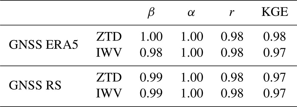
Quite good agreement is obtained, with mean KGE values of 0.98 and 0.97 for the ZTD and IWV, respectively. In addition, we validate the GNSS results with respect to nearby radiosonde measurements at 00:00 and 12:00 UTC for the same period. The radiosonde data are derived from the Integrated Global Radiosonde Archive (IGRA) version 2. We determine a GNSS and radiosonde station pair if their horizontal distance is within 50 km and their height difference is within 100 m. Four station pairs are then determined, namely 0384-GMM00010739, 0389-GMM00010739, 0400-GMM00010739, and BIRK-GMM00010618. For each station pair, the radiosonde ZTD and IWV are calculated by using the integration of vertical profiles from the corresponding GNSS station height. The mean KGE values (0.97) for the GNSS-derived ZTD and IWV with respect to the corresponding radiosonde results are also very high (Table 3).

Figure 4Performance measures for the IWV of PS InSAR vs. GNSS for different subsets of the InSAR domain (see Fig. 1). The term stat_all describes the performance of all 25 GNSS stations in the InSAR domain, and val_5 are the five selected validation stations (cyan dots in Fig. 1) and the individual measures for these five stations, followed by the seasonal analysis of these five stations.
The InSAR-derived IWV results are compared to the GNSS-derived IWV at the GNSS stations. First, the 10 nearest InSAR PS points to the GNSS stations are computed, and a height correction based on ERA5-IWV standard atmospheric height dependencies is applied. In total, 25 GNSS stations are located within the InSAR domain and have sufficient data points. Figure 4 shows the KGE and its constituents for different subsets of the data. The mean values of the KGE over all 25 GNSS stations in the SAR area are presented on top, followed by the mean over the five validation stations, with a superior agreement seen for the latter. The detailed description for each validation station is displayed separately, with the worst performance at station FRI3. At the bottom of the figure, the validation stations data are split into the different seasons, independent of the year, and validated separately. The best results are obtained in autumn, followed by winter and spring, whereas the summer shows the highest differences.
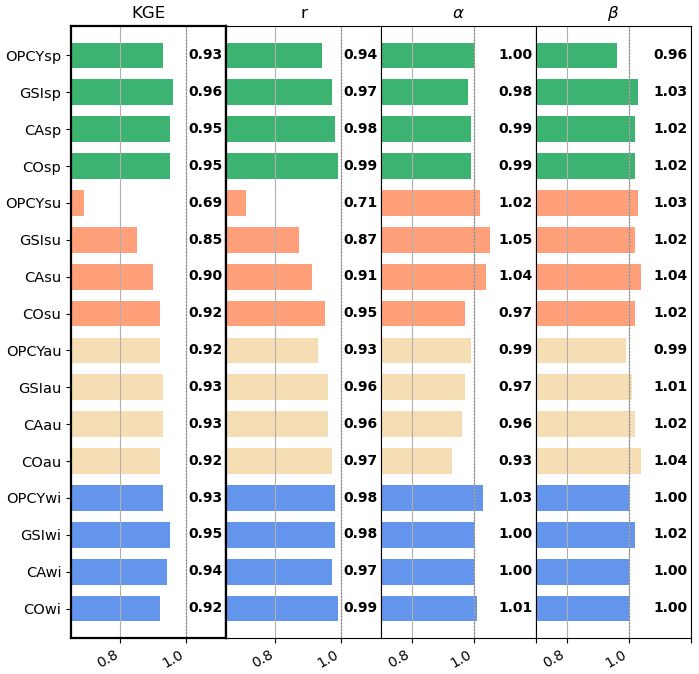
Figure 5Performance measures for IWV of WRF simulations and original, not assimilated, tomography collocation data (CO) vs. five GNSS validation stations. The abbreviations represent the assimilated observations, with OPCY as the simulation without assimilation, GSI as the combined assimilation of GNSS, synoptic, and InSAR data, and CA as the collocation data. The abbreviations sp, su, au, and wi represent the seasons of spring, summer, autumn, and winter.
WRF simulation results are compared to 5 GNSS stations for IWV (Fig. 5) and to 350 stations for precipitation amounts (Fig. 6) for each of the four events. Figure 5 reveals that a high accordance between GNSS stations and the open-cycle simulations already exists for spring, autumn, and winter, with KGE values of approximately 0.93 for IWV. Only in summer is the KGE value below 0.7 due to convective activity. Despite the already high accordance, slight improvements for all seasons are obtained by the assimilation of tomography data (CA) and by the combined assimilation of GNSS, synoptic, and InSAR data (GSI). This is most evident in summer, with the KGEs now larger than 0.85. Original collocation data (CO) show the best performance regarding correlation for all seasons. The KGE of CO is only the best in summer, but there is still a high accordance for the other seasons, similar to the assimilation runs.
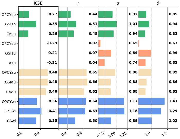
Figure 6Same as Fig. 5 but for precipitation amounts at approx. 350 stations and only for the WRF simulations.
A similar picture is obtained for precipitation (Fig. 6); however, there are much lower KGE values. The best agreement for the open-cycle simulations is obtained in autumn, with the worst again in summer. The assimilation of ZTD only (CA) improved only the simulation results in summer. But, for the joint assimilation of water vapor values and temperature data (GSI), an improvement for every season becomes obvious.
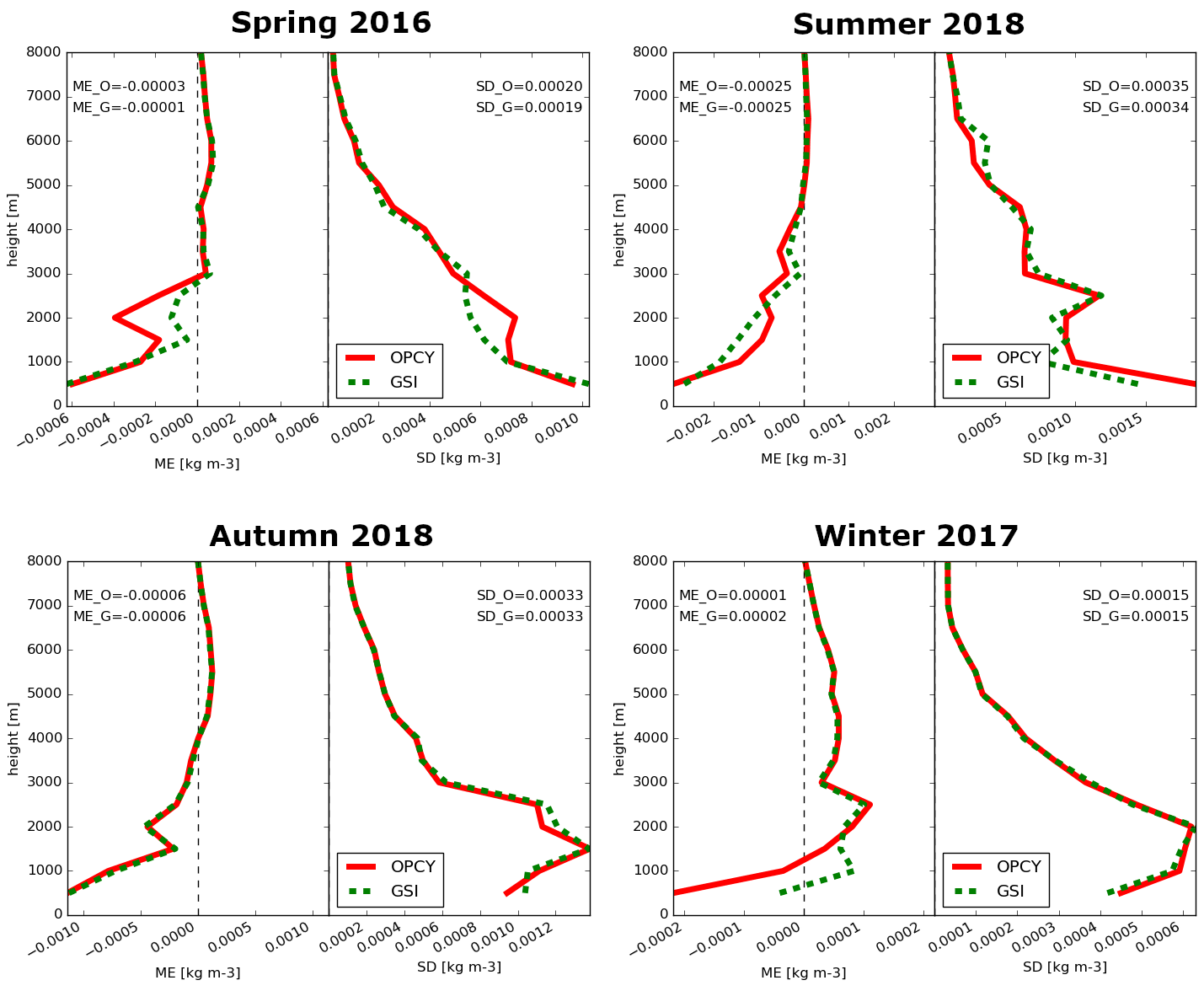
Figure 7Mean error (ME) and standard deviation (SD) of the water vapor density for all seasons, comparing the simulations with the open cycle (solid) and the assimilation of station data (dashed) with radiosonde data for the location of Idar-Oberstein (x-axis range varies for the different seasons).
The vertical distribution of water vapor is evaluated based on profiles of water vapor density (WVD; Sect. A3) with respect to radiosonde observations. In Fig. 7, the mean profiles of WVD from the simulation results are opposed to radiosonde data for Idar-Oberstein. The results for IWV and precipitation are similar for the vertical distribution. In autumn, there are hardly any differences between OPCY and simulations with assimilation, while improvements can be seen in the other seasons. In winter, differences become clear up to a maximum of 2500 m but mainly only up to an altitude of 1500 m. In spring, and especially in summer, however, there are also differences above an altitude of 4000 m. Improvements through assimilation are not uniform for every altitude in every season. But, on average, the results for the simulations with assimilation show a better performance in terms of mean error and standard deviation than without.
A cross-validation between the GNSS-derived IWVs and collocated/interpolated ones using COMEDIE is shown in Fig. 8, where the reference IWVs are shown in continuous lines and the collocated ones in dashed lines. These five stations were not used in the collocation process to derive the parameters that define the functional part of the collocation; therefore, the GNSS- and COMEDIE-derived IWVs can been treated as independent. At first glance, the continuous and dashed curves in Fig. 8 seem to follow a similar pattern. However, from the differences in Fig. 9, we can see that there are some millimeter differences for all five stations for all the events. On humid days and during periods of high IWV variability, a bigger disagreement is obtained, and the smallest differences occur in the winter season. The statistics (mean value and standard deviation) for each station are always below 1 mm for winter, spring, and autumn events; however, the standard deviation of the differences is around 1 mm for the summer events only. On the one hand, this evaluation shows the capabilities of our collocation method to interpolate GNSS-derived IWVs. On the other hand, it is a mean to check the internal consistency of GNSS-derived IWVs of the GURN network.

Figure 8Collocated vs. reference GNSS estimated IWV at five validation stations. Continuous lines represent the reference GNSS station values and dashed lines the ones of collocated data. The colors mark the five different stations.
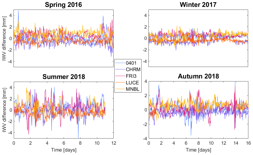
Figure 9Seasonal residuals between reference GNSS estimated and collocated IWV at five validation stations. The colors mark the five different stations.
In Fig. 10, we compare IWV fields between WRF (open-cycle simulation) and COMEDIE for the events in spring 2016, where the differences for one epoch (top panel) and the averaged differences (bottom panel) for all epochs are shown. For every epoch, there are a few millimeters of difference, depending on the pixel (with overall standard deviation at sub-millimeter level), while, in the bottom plot, the difference is smoothed, with an even smaller standard deviation over all epochs and pixels. Furthermore, it is interesting to notice that the differences are not notably larger in the lower-right corner of the grid where the mountainous area is located, meaning that the differences between WRF and COMEDIE are not topographically related.
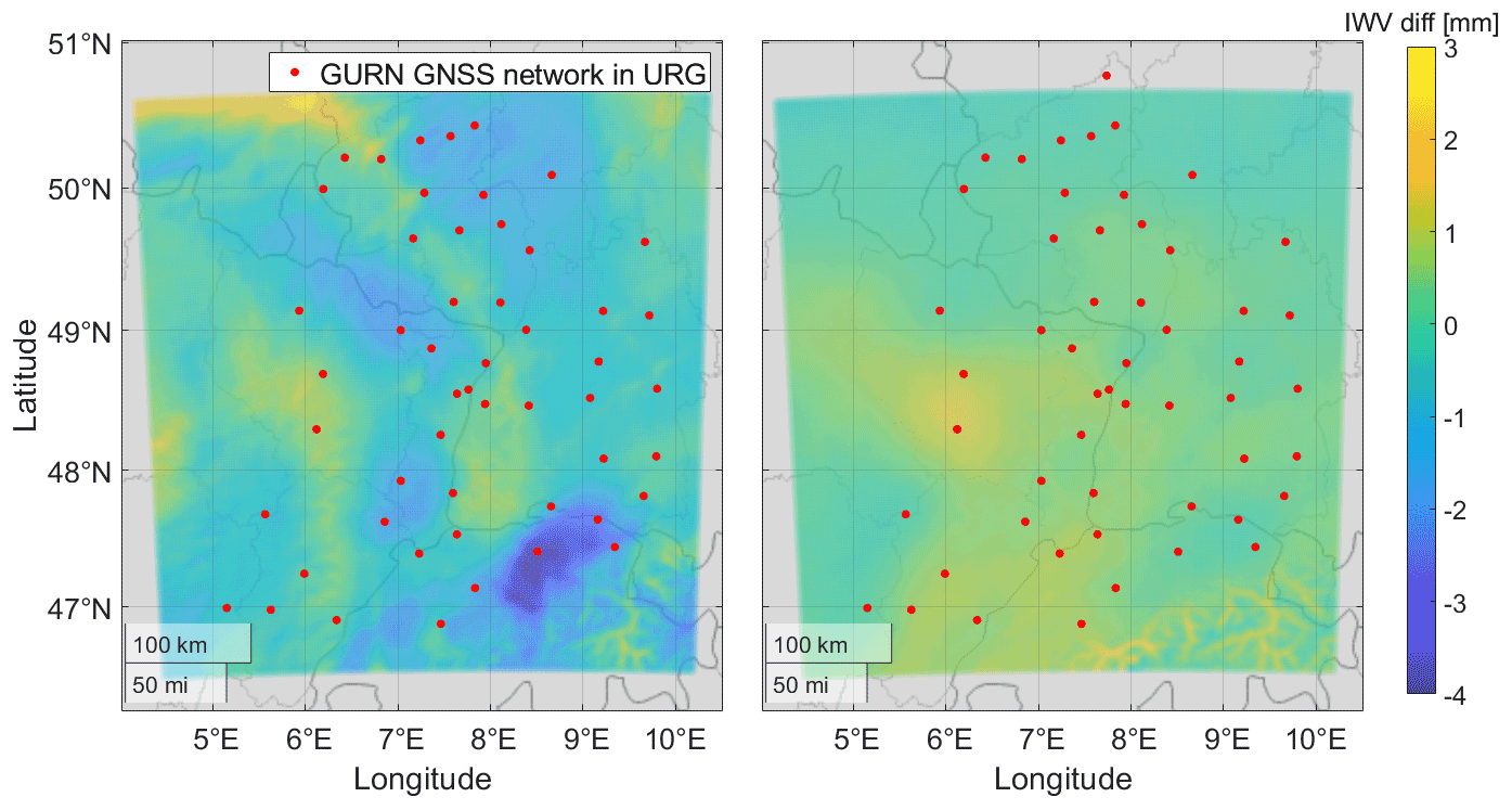
Figure 10Differences between collocated IWVs and WRF model (open-cycle simulation) for spring 2016. In the left subplot, one epoch (11–22 April 2016) is displayed, while the mean over all epochs is shown in the right subplot. The red dots mark the location of GNSS stations used for collocation.
The dataset described in this paper was published on the PANGAEA data publishing platform under https://doi.org/10.1594/PANGAEA.936447 (Fersch et al., 2021). The ERA5 global atmospheric reanalysis data are available at the Copernicus Climate Data service of the European Union (https://doi.org/10.24381/cds.adbb2d47, Hersbach et al., 2018a; https://doi.org/10.24381/cds.bd0915c6, Hersbach et al., 2018b). The WRF model (Skamarock et al., 2008, https://doi.org/10.5065/D68S4MVH) version 3.9.1.1 was used in this study. The source code is available at https://github.com/wrf-model/WRF/releases/tag/V3.9.1.1 (Gill et al., 2017). The GAMIT GNSS data-processing software can be obtained from King (2022).
The Sentinel data are freely available through the Copernicus program (https://scihub.copernicus.eu/; Copernicus, 2020). The formulations of the COMEDIE software and implementations are described in Eckert et al. (1992a, b), Troller (2004), Hurter (2014). The source code is available from the authors upon reasonable request and with the permission of ETH Zurich.
The dataset developed and presented in this work provides a comprehensive, multi-perspective, multi-season, and multi-scale determination of tropospheric water vapor over the study area in the transborder region of Germany, Switzerland, and France. It contains hourly 2D fields of integrated water vapor (IWV) from the various disciplines and 3D fields of water vapor density (WVD) for four multi-week, variable season periods between April 2016 and October 2018 at a spatial resolution of (2.1 km)2. Zenith total delay (ZTD) from GNSS and collocation and refractivities are provided as intermediate products. InSAR-derived double differential slant total delay phases (ddSTDPs) are available for March 2015 to July 2019. The original input data for this work were hourly time series from 66 GNSS stations, hourly ERA5 reanalysis fields from ECMWF, and hourly Sentinel-1A/B InSAR observations.
GNSS-derived IWV is highly accurate and features a high temporal resolution, whereas the InSAR products score with their spatial density. The combination of both by collocation or tomography and the assimilation with regional atmospheric models yields sophisticated descriptions of tropospheric moisture states that cannot be derived from the individual methods alone.
The ECMWF ERA5 global reanalysis depicts a valuable resource for the GNSS-based determination of ZWD and IWV for stations with lacking meteorological observations and likewise for the computation from InSAR. The limited-area WRF simulations for the GURN region benefited from the assimilation of either GNSS, synoptic, InSAR, or collocation data, with the latter leading to slightly inferior results. The strongest impact is seen for the summer event, where levels of IWV are generally high and fluctuations are strong because of convective dynamics. The joint assimilation of water vapor and temperature yields, in particular, a largely better performance of GSI compared to CA.
The presented dataset will be useful for all kinds of studies that require high-resolution information about tropospheric water vapor states and dynamics. In future studies, the spatial coverage could be increased to the continental-scale extent to study the impact of tropospheric water vapor assimilation on the larger scale. Other GNSS systems, such as Galileo or GLONASS, could also be included to provide more observations. The new generation of currently realized microsatellite missions, like Capella X-SAR, will significantly increase the temporal sampling of InSAR-derived tropospheric water vapor products from several days (currently) to less than 1 h (in the future). This will further increase the relevance of InSAR. Although WRF and tomography also provide water vapor profiles, the underlying water vapor measurements are column values only. In the case of very variable humidity conditions, for example, the assimilation of water vapor profiles may further improve the simulations. Finally, the beneficial joint assimilation of energy quantities can be extended by radiation products. Other datasets, such as GNSS radio occulations, can be included into the combination, which can provide complementary information regarding water vapor in the higher troposphere.
A1 Computation of ZWD and IWV with Tm, Ps from ERA5 reanalysis
In order to retrieve IWV from GPS-derived ZTD, we firstly determine the four grid nodes surrounding the GPS station horizontally. We then calculate the related variables (e.g., Ps) of the grid nodes at the station's height. Finally, we calculate the IWV at the station's location by using inverse distance weighting (IDW) interpolation (Jade and Vijayan, 2008). For each grid node, we calculate ZHD according to the Saastamoinen model, as follows (Saastamoinen, 1972):
where Ps is the pressure at the GPS station obtained from reanalysis products in hectopascals (hereafter hPa), ϕs and hs are the stations' latitude and its height above the geoid in meters, respectively. In this process, the following barometric correction formula recommended by the International Civil Aviation Organization (ICAO) is applied:
where P0 is the referential pressures in hPa, with a height of h0 in meters, T0 is the temperature in Kelvins at the height of h0, γ=0.0065 K m−1 is the standard temperature lapse rate, g0=9.80665 m s−2 is the standard acceleration of gravity, and Rd=287.033 J kg−1 K−1 is the gas constant for dry air. Then, we obtain ZWD in millimeters as follows:
Finally, we convert the ZWD into IWV as follows (Bevis et al., 1994):
where ρ=1000 kg m−3, Rw = 461.522 J kg−1 K−1, k21=22.1 K hPa−1, and k3=373 900 K2 hPa−1. Tm is the weighted mean temperature in Kelvins given by the following (Davis et al., 1985):
where e and T are water vapor pressure in hPa and temperature in Kelvins, respectively. The water vapor pressure is given by the following:
whereas esat(T) in hPa and RH denote saturation vapor pressure and relative humidity, respectively. The saturation vapor pressure is estimated using the Tetens formula (IFS CY41R2) as follows:
where a1=611.21 Pa and T0=273.16 K, a3=17.502, and a4=32.19 K are for saturation over water. For the saturation over ice, a3=22.587 and K. As the Tm is integrated from the GPS station height to the highest reanalysis level, the RH and temperature at the station are calculated with linear inter-/extrapolation.
In addition, to assist the estimation of InSAR-derived ZWD, the ZWD in meters obtained from ERA5 pressure level products are calculated as follows:
where Nw is the wet component of refractivity, which is unitless (Davis et al., 1985). This is explained as follows:
Likewise, the ERA5-derived ZTD in meters can be calculated as follows:
where N is the refractivity, which is unitless (Davis et al., 1985). This is explained as follows:
where pd is the pressure of dry air in hPa and k1=77.6 K hPa−1, k2=70.4 K hPa−1, K hPa−1, and k3=373 900 K2 hPa−1.
The ERA5-derived IWV in kilograms per meter squared (kg m−2) can be calculated as follows:
where ρw is the density of water vapor in kilograms per meter cubed (kg m−3).
A2 Computation of water vapor density from collocated IWV
For the retrieval of IWV fields using COMEDIE, we have separately performed the collocation/interpolation of zenith total delays and zenith dry delays and thus computed zenith wet delays as their differences. Using Tm from ERA5, we have obtained the final IWV fields displayed in this paper here.
The retrieval of water vapor density fields has been performed similarly to the retrieval of refractivity fields from ZTDs, as described in Sect. 3.5, where in Eqs. (8) and 11 the ZTDs and refractivities were replaced by IWVs and WVDs, respectively.
A3 Computation of IWV and WVD from WRF data
The integrated water vapor and the water vapor density from WRF is calculated based on the water vapor mixing ratio, temperature, and pressure for the 72 vertical pressure levels. Temperature T is defined as follows:
where TP is the potential perturbation in Kelvins, Tbase=300 K is the base temperature, P is the pressure in hPa, RD=287 J kg−1 K−1 is the gas constant for dry air, and cp = 1004.5 J kg−1 K−1 is heat capacity at constant pressure for dry air.
The integrated water vapor is calculated as the sum of water vapor in the vertical levels as follows:
where QV is the water vapor mixing ratio, dh is the layer thickness in meters, and TV is the virtual temperature of each level in Kelvins. With the following:
where ϵ is the ratio of the gas constants of air, and water vapor is 0.622.
The three-dimensional water vapor density is calculated as follows:

The supplement related to this article is available online at: https://doi.org/10.5194/essd-14-5287-2022-supplement.
BF conceived the paper structure and contributed to all sections. Moreover, BF put together the data collection and organized the publication at PANGAEA. PY created the GNSS dataset, wrote the GNSS-related parts, and performed the calculations of related variables (e.g., Ps, Tm, ZWD, and IWV) from ERA5 reanalysis for the GNSS and InSAR products (Appendix A1). BK created the InSAR-derived data products and wrote the InSAR-related parts together with AS. ES produced the collocation and tomography datasets and wrote the respective parts with GM. AW performed the data assimilation with WRF, created the respective datasets, and authored the corresponding passages. AG, BH, SH, HarK, and HanK contributed to the conception and design of the study. All authors contributed to the writing of the general parts of the paper.
The contact author has declared that none of the authors has any competing interests.
Publisher's note: Copernicus Publications remains neutral with regard to jurisdictional claims in published maps and institutional affiliations.
We would like to thank EOST (École et Observatoire des Sciences de la Terre of the University of Strasbourg and the French National Center for Scientific Research, France) for the collaboration in maintaining the GURN network. Thanks are also given to the GNSS data providers, such as SAPOS (AdV) and GREF (BKG) from Germany, RENAG (CNRS), TERIA, RGP (IGN), and SATINFO from France, swisstopo from Switzerland, and also EPN (EUREF) and IGS. We are also grateful to National Centers for Environmental Information (NCEI), for providing the radiosonde data. We would like to acknowledge the German Meteorological Service (DWD), for supplying us synoptic station data. Furthermore, we thank the PANGAEA data publisher for its excellent service and their help with processing and hosting the dataset developed in this work.
This research has been supported by the Deutsche Forschungsgemeinschaft (grant nos. HE 1433/23-1, HI 1289/11-1, and KU 2090/10-1) and the Schweizerischer Nationalfonds zur Förderung der Wissenschaftlichen Forschung (grant no. 200021E-168952).
This paper was edited by Qingxiang Li and reviewed by Minyan Wang and one anonymous referee.
Almansa, A. F., Cuevas, E., Barreto, Á., Torres, B., García, O. E., García, R. D., Velasco-Merino, C., Cachorro, V. E., Berjón, A., Mallorquín, M., López, C., Ramos, R., Guirado-Fuentes, C., Negrillo, R., and de Frutos, Á. M.: Column Integrated Water Vapor and Aerosol Load Characterization with the New ZEN-R52 Radiometer, Remote Sensing, 12, 1424, https://doi.org/10.3390/rs12091424, 2020. a
Alshawaf, F., Zus, F., Balidakis, K., Deng, Z., Hoseini, M., Dick, G., and Wickert, J.: On the statistical significance of climatic trends estimated from GPS tropospheric time series, J. Geophys. Res.-Atmos., 123, 10–967, https://doi.org/10.1029/2018JD028703, 2018. a
Altamimi, Z., Rebischung, P., Métivier, L., and Collilieux, X.: ITRF2014: A new release of the International Terrestrial Reference Frame modeling nonlinear station motions, J. Geophys. Res.-Sol. Ea., 121, 6109–6131, https://doi.org/10.1002/2016JB013098, 2016. a
Andersson, E., Hólm, E., Bauer, P., Beljaars, A., Kelly, G. A., McNally, A. P., Simmons, A. J., Thépaut, J.-N., and Tompkins, A. M.: Analysis and forecast impact of the main humidity observing systems, Q. J. Roy. Meteorol. Soc., 133, 1473–1485, https://doi.org/10.1002/qj.112, 2007. a
Barker, D., Huang, W., Guo, Y., and Bourgeois, A.: A Three-demiensional Variational (3DVAR) Data Assimilation System for Use With MM5 (No. NCAR/TN-453+STR), University Corporation for Atmospheric Research, 73 pp., https://doi.org/10.5065/D6CF9N1J, 2003. a, b
Barker, D., Huang, W., Guo, Y., Bourgeois, A., and Xiao, A.: A Three-Dimensional Variational Data Assimilation System for MM5: Implementation and Initial Results, Mon. Weather Rev., 132, 897–914, https://doi.org/10.1175/1520-0493(2004)132<0897:ATVDAS>2.0.CO;2, 2004. a, b, c
Bevis, M., Businger, S., Herring, T. A., Rocken, C., Anthes, R. A., and Ware, R. H.: GPS meteorology: Remote sensing of atmospheric water vapor using the global positioning system, J. Geophys. Res., 97, 15787–15801, https://doi.org/10.1029/92JD01517, 1992. a, b
Bevis, M., Businger, S., Chiswell, S., Herring, T. A., Anthes, R. A., Rocken, C., and Ware, R. H.: GPS meteorology: Mapping zenith wet delays onto precipitable water, J. Appl. Meteorol., 33, 379–386, 1994. a, b
Boehm, J., Werl, B., and Schuh, H.: Troposphere mapping functions for GPS and very long baseline interferometry from European Centre for Medium-Range Weather Forecasts operational analysis data, J. Geophys. Res.-Sol. Ea., 111, B02406, https://doi.org/10.1029/2005JB003629, 2006. a
Boniface, K., Ducrocq, V., Jaubert, G., Yan, X., Brousseau, P., Masson, F., Champollion, C., Chéry, J., and Doerflinger, E.: Impact of high-resolution data assimilation of GPS zenith delay on Mediterranean heavy rainfall forecasting, Ann. Geophys., 27, 2739–2753, https://doi.org/10.5194/angeo-27-2739-2009, 2009. a
Chen, G. and Herring, T.: Effects of atmospheric azimuthal asymmetry on the analysis of space geodetic data, J. Geophys. Res.-Sol. Ea., 102, 20489–20502, 1997. a
Copernicus: Copernicus Sentinel data [2015–2019], https://scihub.copernicus.eu/, last access: 22 October 2020. a
Davis, J., Herring, T., Shapiro, I., Rogers, A., and Elgered, G.: Geodesy by radio interferometry: Effects of atmospheric modeling errors on estimates of baseline length, Radio Sci., 20, 1593–1607, https://doi.org/10.1029/RS020i006p01593, 1985. a, b, c, d
Dee, D. P., Uppala, S. M., Simmons, A. J., Berrisford, P., Poli, P., Kobayashi, S., Andrae, U., Balmaseda, M. A., Balsamo, G., Bauer, P., Bechtold, P., Beljaars, A. C. M., van de Berg, L., Bidlot, J., Bormann, N., Delsol, C., Dragani, R., Fuentes, M., Geer, A. J., Haimberger, L., Healy, S. B., Hersbach, H., Hólm, E. V., Isaksen, L., Kållberg, P., Köhler, M., Matricardi, M., McNally, A. P., Monge-Sanz, B. M., Morcrette, J.-J., Park, B.-K., Peubey, C., de Rosnay, P., Tavolato, C., Thépaut, J.-N., and Vitart, F.: The ERA-Interim reanalysis: configuration and performance of the data assimilation system, Q. J. Roy. Meteor. Soc., 137, 553–597, https://doi.org/10.1002/qj.828, 2011. a
Divakarla, M. G., Barnet, C. D., Goldberg, M. D., McMillin, L. M., Maddy, E., Wolf, W., Zhou, L., and Liu, X.: Validation of Atmospheric Infrared Sounder temperature and water vapor retrievals with matched radiosonde measurements and forecasts, J. Geophys. Res., 111, D09S15, https://doi.org/10.1029/2005JD006116, 2006. a
Dudhia, J.: Numericall study of convection observed during the Winterl Monsoonl Experimentl using a mesoscale two-dimensional model, J. Atmos. Sci., 46, 3077–3107, https://doi.org/10.1175/1520-0469(1989)046<3077:NSOCOD>2.0.CO;2, 1989. a
DWD: DWD synoptic data, https://www.dwd.de/EN/climate_environment/cdc/cdc_node_en.html (last access: 28 November 2022), https://opendata.dwd.de/climate_environment/CDC/observations_germany, last access: 4 December 2020. a
Eckert, V., Cocard, M., and Geiger, A.: COMEDIE: (Collocation of meteorological data for interpretation and estimation of tropospheric pathdelays) Teil I: Konzepte, Teil II: Resultate, Technical Report 194, ETH Zürich, Grauer Bericht, 1992a. a, b, c, d
Eckert, V., Cocard, M., and Geiger, A.: COMEDIE: (Collocation of meteorological data for interpretation and estimation of tropospheric pathdelays) Teil III: Software, Technical Report 195, ETH Zürich, Grauer Bericht, 1992b. a, b, c
ECMWF: ERA5 reanalysis data, https://www.ecmwf.int/en/forecasts/datasets/reanalysis-datasets/era5, last access: 4 December 2020. a, b
Efron, B.: Bootstrap Methods: Another Look at the Jackknife, Ann. Stat., 7, 1–26, https://doi.org/10.1214/aos/1176344552, 1979. a
Feltz, W. F., Smith, W. L., Howell, H. B., Knuteson, R. O., Woolf, H., and Revercomb, H. E.: Near-Continuous Profiling of Temperature, Moisture, and Atmospheric Stability Using the Atmospheric Emitted Radiance Interferometer (AERI), J. Appl. Meteorol., 42, 584–597, https://doi.org/10.1175/1520-0450(2003)042<0584:npotma>2.0.co;2, 2003. a
Ferretti, A., Prati, C., and Rocca, F.: Permanent scatterers in SAR interferometry, IEEE T. Geosci. Remote, 39, 8–20, https://doi.org/10.1109/36.898661, 2001. a
Fersch, B., Senatore, A., Adler, B., Arnault, J., Mauder, M., Schneider, K., Völksch, I., and Kunstmann, H.: High-resolution fully coupled atmospheric–hydrological modeling: a cross-compartment regional water and energy cycle evaluation, Hydrol. Earth Syst. Sci., 24, 2457–2481, https://doi.org/10.5194/hess-24-2457-2020, 2020. a
Fersch, B., Kamm, B., Shehaj, E., Wagner, A., Yuan, P., Möller, G., Schenk, A., Geiger, A., Hinz, S., Kutterer, H., and Kunstmann, H.: A comprehensive high resolution data collection for tropospheric water vapor assessment for the Upper Rhine Graben, Germany, PANGAEA [data set], https://doi.org/10.1594/PANGAEA.936447, 2021. a, b, c
Furumoto, J., Kurimoto, K., and Tsuda, T.: Continuous Observations of Humidity Profiles with the MU Radar–RASS Combined with GPS and Radiosonde Measurements, J. Atmos. Ocean. Tech., 20, 23–41, https://doi.org/10.1175/1520-0426(2003)020<0023:COOHPW>2.0.CO;2, 2003. a
Gallus, W. A. and Segal, M.: Impact of Improved Initialization of Mesoscale Features on Convective System Rainfall in 10-km Eta Simulations, Weather Forecast., 16, 680–696, https://doi.org/10.1175/1520-0434(2001)016<0680:ioiiom>2.0.co;2, 2001. a
Giannaros, C., Kotroni, V., Lagouvardos, K., Giannaros, T. M., and Pikridas, C.: Assessing the Impact of GNSS ZTD Data Assimilation into the WRF Modeling System during High-Impact Rainfall Events over Greece, Remote Sensing, 12, 383, https://doi.org/10.3390/rs12030383, 2020. a
Gill, D., Dudhia, J. Wang, W.: WRF-ARW Modeling System, GitHub, https://github.com/wrf-model/WRF/releases/tag/V3.9.1.1 (last access: 29 November 2022), 2017. a
Giorgi, F.: Thirty Years of Regional Climate Modeling: Where Are We and Where Are We Going next?, J. Geophys. Res.-Atmos., 124, 5696–5723, https://doi.org/10.1029/2018JD030094, 2019. a
González, A., Expósito, F. J., Pérez, J. C., Díaz, J. P., and Taima, D.: Verification of precipitable water vapour in high-resolution WRF simulations over a mountainous archipelago, Q. J. Roy. Meteor. Soc., 139, 2119–2133, https://doi.org/10.1002/qj.2092, 2013. a
Gupta, H., Kling, H., Yilmaz, K., and Martinez, G.: Decomposition of the Mean Squared Error and NSE Performance Criteria: Implications for Improving Hydrological Modelling, J. Hydrol., 377, 80–91, https://doi.org/10.1016/j.jhydrol.2009.08.003, 2009. a
Hanssen, R. F.: Radar interferometry – Data Interpretation and Error Analysis, vol. 2 of Remote Sensing and Digital Image Processing, Springer Netherlands, Dordrecht, https://doi.org/10.1007/0-306-47633-9, 2001. a, b
Herring, T. A., King, R. W., Floyd, M. A., and McClusky, S. C.: Introduction to GAMIT/GLOBK, Release 10.7, Massachusetts Institute of Technology, Cambridge, Massachusetts, http://geoweb.mit.edu/gg/Intro_GG.pdf (last access: 28 November 2022), 2018. a
Hersbach, H., Bell, B., Berrisford, P., Biavati, G., Horányi, A., Muñoz Sabater, J., Nicolas, J., Peubey, C., Radu, R., Rozum, I., Schepers, D., Simmons, A., Soci, C., Dee, D., and Thépaut, J.-N.: ERA5 hourly data on single levels from 1959 to present, Copernicus Climate Change Service (C3S) Climate Data Store (CDS) [data set], https://doi.org/10.24381/cds.adbb2d47, 2018a. a
Hersbach, H., Bell, B., Berrisford, P., Biavati, G., Horányi, A., Muñoz Sabater, J., Nicolas, J., Peubey, C., Radu, R., Rozum, I., Schepers, D., Simmons, A., Soci, C., Dee, D., and Thépaut, J.-N.: ERA5 hourly data on pressure levels from 1959 to present, Copernicus Climate Change Service (C3S) Climate Data Store (CDS) [data set], https://doi.org/10.24381/cds.bd0915c6, 2018b. a
Hersbach, H., Bell, B., Berrisford, P., Hirahara, S., Horányi, A., Muñoz-Sabater, J., Nicolas, J., Peubey, C., Radu, R., Schepers, D., Simmons, A., Soci, C., Abdalla, S., Abellan, X., Balsamo, G., Bechtold, P., Biavati, G., Bidlot, J., Bonavita, M., De Chiara, G., Dahlgren, P., Dee, D., Diamantakis, M., Dragani, R., Flemming, J., Forbes, R., Fuentes, M., Geer, A., Haimberger, L., Healy, S., Hogan, R. J., Hólm, E., Janisková, M., Keeley, S., Laloyaux, P., Lopez, P., Lupu, C., Radnoti, G., de Rosnay, P., Rozum, I., Vamborg, F., Villaume, S., and Thépaut, J.-N.: The ERA5 Global Reanalysis, Q. J. Roy. Meteor. Soc., 146, 1999–2049, https://doi.org/10.1002/qj.3803, 2020. a
Heublein, M. E. A.: GNSS and InSAR based water vapor tomography: A Compressive Sensing solution, PhD thesis, Karlsruhe Institute of Technology, https://doi.org/10.5445/IR/1000093403, 2019. a
Hong, S. and Lim, J. J.: The WRF single-moment 6–-lass microphysics scheme (WSM6), J. Korean Meteor. Soc., 42, 129–151, 2006. a
Hong, S., Noh, Y., and Dudhia, J.: A new vertical diffusion package with an explicit treatment of entrainment processes, Mon. Weather Rev., 134, 2318–2341, https://doi.org/10.1175/MWR3199.1, 2006. a
Hooper, A., Segall, P., and Zebker, H.: Persistent scatterer interferometric synthetic aperture radar for crustal deformation analysis, with application to Volcán Alcedo, Galápagos, J. Geophys. Res., 112, B07407, https://doi.org/10.1029/2006JB004763, 2007. a
Hooper, A., Bekaert, D., Spaans, K., and Arikan, M.: Recent advances in SAR interferometry time series analysis for measuring crustal deformation, Tectonophysics, 514–517, 1–13, https://doi.org/10.1016/j.tecto.2011.10.013, 2012. a
Hurter, F.: GNSS meteorology in spatially dense networks, PhD thesis, ETH Zurich, https://doi.org/10.3929/ethz-a-010276927, 2014. a, b, c, d
Ide, K., Ghil, M., and Lorenc, A.: Unified Notation for Data Assimilation: Operational, Sequential and Variational, J. Meteorol. Soc. Jpn., 75, 181–189, https://doi.org/10.2151/jmsj1965.75.1B_181, 1999. a
Jade, S. and Vijayan, M.: GPS-based atmospheric precipitable water vapor estimation using meteorological parameters interpolated from NCEP global reanalysis data, J. Geophys. Res.-Atmos., 113, D03106, https://doi.org/10.1029/2007JD008758, 2008. a
Jiang, X., Li, J., Li, Z., Xue, Y., Di, D., Wang, P., and Li, J.: Evaluation of Environmental Moisture from NWP Models with Measurements from Advanced Geostationary Satellite Imager – A Case Study, Remote Sensing, 12, 670, https://doi.org/10.3390/rs12040670, 2020. a
Jin, S., Feng, G., and Gleason, S.: Remote sensing using GNSS signals: Current status and future directions, Adv. Space Res., 47, 1645–1653, https://doi.org/10.1016/j.asr.2011.01.036, 2011. a
Jochum, A. M., Camino, E. R., de Bruin, H. A. R., and Holtslag, A. A. M.: Performance of HIRLAM in a Semiarid Heterogeneous Region: Evaluation of the Land Surface and Boundary Layer Description Using EFEDA Observations, Mon. Weather Rev., 132, 2745–2760, https://doi.org/10.1175/mwr2820.1, 2004. a
Jones, J., Guerova, G., Douša, J., Dick, G., de Haan, S., Pottiaux, E., and van Malderen, R.: Advanced GNSS Tropospheric Products for Monitoring Severe Weather Events and Climate, COST action ES1206 final action dissemination report, 563 pp., https://doi.org/10.1007/978-3-030-13901-8, 2019. a
King, R. W.: GAMIT/GLOBK, http://geoweb.mit.edu/gg/, last access: 4 January 2022. a
Klanner, L., Höveler, K., Khordakova, D., Perfahl, M., Rolf, C., Trickl, T., and Vogelmann, H.: A powerful lidar system capable of 1 h measurements of water vapour in the troposphere and the lower stratosphere as well as the temperature in the upper stratosphere and mesosphere, Atmos. Meas. Tech., 14, 531–555, https://doi.org/10.5194/amt-14-531-2021, 2021. a
Kunz, A., Spelten, N., Konopka, P., Müller, R., Forbes, R. M., and Wernli, H.: Comparison of Fast In situ Stratospheric Hygrometer (FISH) measurements of water vapor in the upper troposphere and lower stratosphere (UTLS) with ECMWF (re)analysis data, Atmos. Chem. Phys., 14, 10803–10822, https://doi.org/10.5194/acp-14-10803-2014, 2014. a
Leontiev, A. and Reuveni, Y.: Augmenting GPS IWV estimations using spatio-temporal cloud distribution extracted from satellite data, Sci. Rep., 8, 14785, https://doi.org/10.1038/s41598-018-33163-x, 2018. a
Lindenbergh, R., Keshin, M., van der Marel, H., and Hanssen, R.: High resolution spatio‐temporal water vapour mapping using GPS and MERIS observations, Int. J. Remote Sens., 29, 2393–2409, https://doi.org/10.1080/01431160701436825, 2008. a
Lindskog, M., Ridal, M., Thorsteinsson, S., and Ning, T.: Data assimilation of GNSS zenith total delays from a Nordic processing centre, Atmos. Chem. Phys., 17, 13983–13998, https://doi.org/10.5194/acp-17-13983-2017, 2017. a
Löhnert, U., Turner, D. D., and Crewell, S.: Ground-Based Temperature and Humidity Profiling Using Spectral Infrared and Microwave Observations. Part I: Simulated Retrieval Performance in Clear-Sky Conditions, J. Appl. Meteorol. Clim., 48, 1017–1032, https://doi.org/10.1175/2008jamc2060.1, 2009. a
Massaro, G., Stiperski, I., Pospichal, B., and Rotach, M. W.: Accuracy of retrieving temperature and humidity profiles by ground-based microwave radiometry in truly complex terrain, Atmos. Meas. Tech., 8, 3355–3367, https://doi.org/10.5194/amt-8-3355-2015, 2015. a
Mateus, P., Tomé, R., Nico, G., and Catalao, J.: Three-Dimensional Variational Assimilation of InSAR PWV Using the WRFDA Model, IEEE T. Geosci. Remote, 12, 7323–7330, https://doi.org/10.1109/TGRS.2016.2599219, 2016. a
Mateus, P., Miranda, P. M. A., Nico, G., and Catalao, J.: Continuous Multitrack Assimilation of Sentinel-1 Precipitable Water Vapor Maps for Numerical Weather Prediction: How Far Can We Go With Current InSAR Data?, J. Geophys. Res.-Atmos., 126, e2020JD034171, https://doi.org/10.1029/2020JD034171, 2021. a, b
Mayer, M., Knöpfler, A., Heck, B., Masson, F., Ulrich, P., and Ferhat, G.: GURN (GNSS Upper Rhine Graben Network): Research Goals and First Results of a Transnational Geo-scientific Network, in: Geodesy for Planet Earth, edited by: Kenyon, S., Pacino, M. C., and Marti, U., Springer Berlin Heidelberg, Berlin, Heidelberg, 673–681, https://doi.org/10.1007/978-3-642-20338-1_83, 2012. a
Mlawer, E. J., Taubman, S. J., Brown, P. D., Iacono, M. J., and Clough, S. A.: Radiative transfer for inhomogeneous atmospheres: RRTM, a validated correlated-k model for the longwave, J. Geophys. Res., 102, 16663–16682, https://doi.org/10.1029/97JD00237, 1997. a
Moeller, G.: Reconstruction of 3D wet refractivity fields in the lower atmosphere along bended GNSS signal paths, Phd thesis, TU Wien, Department of Geodesy and Geoinformation, 196 pp., http://repositum.tuwien.ac.at/obvutwoa/download/pdf/2284850 (last access: 28 November 2022), 2017. a
Ning, T., Wang, J., Elgered, G., Dick, G., Wickert, J., Bradke, M., Sommer, M., Querel, R., and Smale, D.: The uncertainty of the atmospheric integrated water vapour estimated from GNSS observations, Atmos. Meas. Tech., 9, 79–92, https://doi.org/10.5194/amt-9-79-2016, 2016. a
Pacione, R. and Douša, J.: SINEX-TRO V2. 00 format description, COST Action ES1206 Final Action Dissemination Report, edited by: Jones, J., Guerova, G., Douša, J., Dick, G., de Haan, S., Pottiaux, E., and van Malderen, R., 537–563, https://doi.org/10.1007/978-3-030-13901-8, 2017. a
Parrish, D. F. and Derber, J. C.: The National Meteorological Center's Spectral Statistical-Interpolation Analysis System, Mon. Weather Rev., 120, 1747–1763, https://doi.org/10.1175/1520-0493(1992)120<1747:TNMCSS>2.0.CO;2, 1992. a
Petit, G. and Luzum, B. (Eds.): IERS Conventions (2010), IERS Technical Note; 36, Frankfurt am Main: Verlag des Bundesamts für Kartographie und Geodäsie, 179 pp., ISBN 3-89888-989-6, https://www.iers.org/IERS/EN/Publications/TechnicalNotes/tn36.html (last access: 28 November 2022), 2010. a
Pichelli, E., Ferretti, R., Cimini, D., Panegrossi, G., Perissin, D., Pierdicca, N., Member, S., Rocca, F., and Rommen, B.: InSAR Water Vapor Data Assimilation into Mesoscale Model MM5: Technique and Pilot Study, IEEE J. Sel. Top. Appl., 8, 3859–3875, https://doi.org/10.1109/JSTARS.2014.2357685, 2015. a
Poli, P., Healy, S., Rabier, F., and Pailleux, J.: Preliminary assessment of the scalability of GPS radio occultations impact in numerical weather prediction, Geophys. Res. Lett., 35, L23811, https://doi.org/10.1029/2008GL035873, 2008. a
Pondeca, M. and Zou, X.: A Case Study of the Variational Assimilation of GPS Zenith Delay Observations into a Mesoscale Model, J. Appl. Meteorol., 40, 1559–1576, https://doi.org/10.1175/1520-0450(2001)040<1559:ACSOTV>2.0.CO;2, 2001. a
Pospichal, B. and Crewell, S.: Boundary layer observations in West Africa using a novel microwave radiometer, Meteorol. Z., 16, 513–523, https://doi.org/10.1127/0941-2948/2007/0228, 2007. a
Prein, A. F., Langhans, W., Fosser, G., Ferrone, A., Ban, N., Goergen, K., Keller, M., Tölle, M., Gutjahr, O., Feser, F., Brisson, E., Kollet, S., Schmidli, J., Lipzig, N. P. M., and Leung, R.: A review on regional convection-permitting climate modeling: Demonstrations, prospects, and challenges, Rev. Geophys., 53, 323–361, https://doi.org/10.1002/2014RG000475, 2015. a
Randel, D. L., Greenwald, T. J., Haar, T. H. V., Stephens, G. L., Ringerud, M. A., and Combs, C. L.: A New Global Water Vapor Dataset, B. Am. Meteorol. Soc., 77, 1233–1246, https://doi.org/10.1175/1520-0477(1996)077<1233:angwvd>2.0.co;2, 1996. a
Reale, A., Tilley, F., Ferguson, M., and Allegrino, A.: NOAA operational sounding products for advanced TOVS, Int. J. Remote Sens., 29, 4615–4651, https://doi.org/10.1080/01431160802020502, 2008. a
Rocken, C., Kuo, Y.-H., Sokolovskiy, S. V., and Anthes, R. A.: The ROCSAT-3/COSMIC mission and applications of GPS radio occultation data to weather and climate, in: Remote Sensing Applications of the Global Positioning System, edited by: Bevis, M., Shoji, Y., and Businger, S., SPIE, https://doi.org/10.1117/12.566544, 2004. a
Saastamoinen, J.: Atmospheric correction for the troposphere and stratosphere in radio ranging satellites, in: The Use of Artificial Satellites for Geodesy, edited by: Henriksen, S. W., Mancini, A., and Chovitz, B. H., 15, 247–251, https://doi.org/10.1029/GM015p0247, 1972. a, b
Schaer, S.: Mapping and predicting the Earth's ionosphere using the Global Positioning System, Geodätisch-geophysikalische Arbeiten in der Schweiz, 59, 205 pp., 1999. a
Schmid, R., Dach, R., Collilieux, X., Jäggi, A., Schmitz, M., and Dilssner, F.: Absolute IGS antenna phase center model igs08. atx: status and potential improvements, J. Geodesy, 90, 343–364, https://doi.org/10.1007/s00190-015-0876-3, 2016. a
Shehaj, E., Wilgan, K., Frey, O., and Geiger, A.: A collocation framework to retrieve tropospheric delays from a combination of GNSS and InSAR, Navigation, 67, 823–842, https://doi.org/10.1002/navi.398, 2020. a, b, c
Shi, L., Matthews, J., peng Ho, S., Yang, Q., and Bates, J.: Algorithm Development of Temperature and Humidity Profile Retrievals for Long-Term HIRS Observations, Remote Sensing, 8, 280, https://doi.org/10.3390/rs8040280, 2016. a
Simmons, A. and Gibson, J.: The era-40 project plan, ERA-40 project report series 1, ECMWF, Reading, United Kingdom, https://www.ecmwf.int/node/12272 (last access: 28 November 2022), 2000. a
Skamarock, W. C. and Klemp, J. B.: A time-split nonhydrostatic atmospheric model for weather research and forecasting applications, J. Comput. Phys., 227, 3465–3485, https://doi.org/10.1016/j.jcp.2007.01.037, 2008. a
Skamarock, W. C., Klemp, J. B., Dudhia, J., Gill, D. O., Barker, D. M., Duda, M. G., Huang, X.-Y., Wang, W., and Powers, J. G.: A Description of the Advanced Research WRF Version 3, NCAR Tech. Note NCAR/TN-475+STR, 113 pp., https://doi.org/10.5065/D68S4MVH, 2008. a
SNAP: S1TBX – ESA Sentinel-1 Toolbox v8.0.1, http://step.esa.int/, last access: 1 February 2021. a
Steinke, S., Eikenberg, S., Löhnert, U., Dick, G., Klocke, D., Di Girolamo, P., and Crewell, S.: Assessment of small-scale integrated water vapour variability during HOPE, Atmos. Chem. Phys., 15, 2675–2692, https://doi.org/10.5194/acp-15-2675-2015, 2015. a
Steinke, S., Wahl, S., and Crewell, S.: Benefit of high resolution COSMO reanalysis: The diurnal cycle of column-integrated water vapor over Germany, Meteorol. Z., 28, 165–177, https://doi.org/10.1127/metz/2019/0936, 2019. a
Stevens, B. and Bony, S.: Water in the atmosphere, Physics Today, 66, 29–34, https://doi.org/10.1063/PT.3.2009, 2013. a
Teunissen, P. and Montenbruck, O.: Springer Handbook of Global Navigation Satellite Systems, Springer, https://doi.org/10.1007/978-3-319-42928-1, 2017. a
Thébault, E., Finlay, C. C., Beggan, C. D., Alken, P., Aubert, J., Barrois, O., Bertrand, F., Bondar, T., Boness, A., Brocco, L., Canet, E., Chambodut, A., Chulliat, A., Coïsson, P., Civet, F., Du, A., Fournier, A., Fratter, I., Gillet, N., Hamilton, B., Hamoudi, M., Hulot, G., Jager, T., Korte, M., Kuang, W., Lalanne, X., Langlais, B., Léger, J.-M., Lesur, V., Lowes, F. J., Macmillan, S., Mandea, M., Manoj, C., Maus, S., Olsen, N., Petrov, V., Ridley, V., Rother, M., Sabaka, T. J., Saturnino, D., Schachtschneider, R., Sirol, O., Tangborn, A., Thomson, A., Tøffner-Clausen, L., Vigneron, P., Wardinski, I., and Zvereva, T.: International geomagnetic reference field: the 12th generation, Earth Planet. Space, 67, 1–19, 2015. a
Troller, M.: GPS based determination of the integrated and spatially distributed water vapor in the troposphere, PhD thesis, ETH Zurich, https://doi.org/10.3929/ethz-a-004796376, 2004. a
Vogelmann, H., Sussmann, R., Trickl, T., and Reichert, A.: Spatiotemporal variability of water vapor investigated using lidar and FTIR vertical soundings above the Zugspitze, Atmos. Chem. Phys., 15, 3135–3148, https://doi.org/10.5194/acp-15-3135-2015, 2015. a
Wagner, A., Heinzeller, D., Wagner, S., Rummler, T., and Kunstmann, H.: Explicit Convection and Scale-Aware Cumulus Parameterizations: High-Resolution Simulations over Areas of Different Topography in Germany, Mon. Weather Rev., 146, 1925–1944, https://doi.org/10.1175/MWR-D-17-0238.1, 2018. a
Wagner, A., Fersch, B., Yuan, P., Rummler, T., and Kunstmann, H.: Assimilation of GNSS and Synoptic Data in a Convection Permitting Limited Area Model: Improvement of Simulated Tropospheric Water Vapor Content, Front. Earth Sci., 10, 869504, https://doi.org/10.3389/feart.2022.869504, 2022. a, b
Wang, J., Zhang, L., and Dai, A.: Global estimates of water-vapor-weighted mean temperature of the atmosphere for GPS applications, J. Geophys. Res.-Atmos., 110, D21101, https://doi.org/10.1029/2005JD006215, 2005. a
Yuan, P., Hunegnaw, A., Alshawaf, F., Awange, J., Klos, A., Teferle, F. N., and Kutterer, H.: Feasibility of ERA5 integrated water vapor trends for climate change analysis in continental Europe: An evaluation with GPS (1994–2019) by considering statistical significance, Remote Sens. Environ., 260, 112416, https://doi.org/10.1016/j.rse.2021.112416, 2021. a
Zhou, L., Lin, S.-J., Chen, J.-H., Harris, L. M., Chen, X., and Rees, S. L.: Toward Convective-Scale Prediction within the Next Generation Global Prediction System, B. Am. Meteorol. Soc., 100, 1225–1243, https://doi.org/10.1175/bams-d-17-0246.1, 2019. a
Zhu, M., Liu, Z., and Hu, W.: Observing Water Vapor Variability During Three Super Typhoon Events in Hong Kong Based on GPS Water Vapor Tomographic Modeling Technique, J. Geophys. Res.-Atmos., 125, e2019JD032318, https://doi.org/10.1029/2019JD032318, 2020. a
- Abstract
- Introduction
- Methods of tropospheric water vapor determination
- Tropospheric water vapor dataset
- Data evaluation and cross-comparison
- Code and data availability
- Conclusions
- Appendix A: Conversion and computation details
- Appendix B: Abbreviations
- Author contributions
- Competing interests
- Disclaimer
- Acknowledgements
- Financial support
- Review statement
- References
- Supplement