the Creative Commons Attribution 4.0 License.
the Creative Commons Attribution 4.0 License.
 | 11 Nov 2022
Downscaled hyper-resolution (400 m) gridded datasets of daily precipitation and temperature (2008–2019) for the East–Taylor subbasin (western United States)
Dipankar Dwivedi
James B. Brown
Carl I. Steefel
High-resolution gridded datasets of meteorological variables are needed in order to resolve fine-scale hydrological gradients in complex mountainous terrain. Across the United States, the highest available spatial resolution of gridded datasets of daily meteorological records is approximately 800 m. This work presents gridded datasets of daily precipitation and mean temperature for the East–Taylor subbasin (in the western United States) covering a 12-year period (2008–2019) at a high spatial resolution (400 m). The datasets are generated using a downscaling framework that uses data-driven models to learn relationships between climate variables and topography. We observe that downscaled datasets of precipitation and mean temperature exhibit smoother spatial gradients (while preserving the spatial variability) when compared to their coarser counterparts. Additionally, we also observe that when downscaled datasets are upscaled to the original resolution (800 m), the mean residual error is almost zero, ensuring no bias when compared with the original data. Furthermore, the downscaled datasets are observed to be linearly related to elevation, which is consistent with the methodology underlying the original 800 m product. Finally, we validate the spatial patterns exhibited by downscaled datasets via an example use case that models lidar-derived estimates of snowpack. The presented dataset constitutes a valuable resource to resolve fine-scale hydrological gradients in the mountainous terrain of the East–Taylor subbasin, which is an important study area in the context of water security for the southwestern United States and Mexico. The dataset is publicly available at https://doi.org/10.15485/1822259 (Mital et al., 2021).
- Article
(4792 KB) - Full-text XML
-
Supplement
(2948 KB) - BibTeX
- EndNote


Water resources are under increasing stresses due to Earth system change and increasing demand for clean water, food, and energy (Vörösmarty et al., 2010). The stresses on water availability and quality are felt through watersheds as they are the fundamental functional units of the Earth's surface that integrate the effects of vegetation, fluvial systems, soils and subsurface on water resources (National Research Council, 1999). Sustainable management of water resources, therefore, requires quantitative modeling efforts at the river basin scale. Such efforts involve the use of land-surface and ecohydrological models which need access to climate forcing via gridded datasets of meteorological variables. Across the United States, the highest available spatial resolution of gridded datasets of daily meteorological records is approximately 800 m (Daly et al., 2008) to 1 km (Thornton et al., 2020). This resolution does not allow models to resolve fine-scale gradients of hydro-biogeochemical processes, which introduces uncertainty associated with predicting response of water resources to various drivers such as wildfire, drought, floods, land-use change, extreme weather, sea-level rise, and climate change (e.g., Singh, 1997; Cotter et al., 2003; Beven et al., 2015). Consequently, there is a need to generate gridded datasets of meteorological variables at hyper-resolutions. In this work, we define hyper-resolutions as spatial resolutions that are of the order of a few hundred meters.
It is possible to obtain hyper-resolution gridded observations of meteorological variables. For example, precipitation can be measured at a resolution of 100 m via X-band radar (e.g., Feldman et al., 2021). However, high measurement cost implies that such data have limited spatial and temporal extent. This leaves us with two possible approaches to generate hyper-resolution gridded datasets that have large spatial and temporal extents: (i) spatial interpolation of point measurements or (ii) spatial downscaling of existing lower-resolution datasets. Spatial interpolation of point measurements requires a high density of stations for high-resolution gridding to adequately capture the climatological variability (Bierkens, 2015; Beven et al., 2015). For instance, a resolution of 1 km needs a station every 1×1 km (Haylock et al., 2008). Since such a high station density is not feasible, interpolation approaches typically incorporate physiographic and climatological information in their methodologies while generating gridded datasets at high spatial resolutions (e.g., Daly et al., 2008; Thornton et al., 2021; Lussana et al., 2019; Crespi et al., 2021; Škrk et al., 2021). A general lack of knowledge about weather patterns at fine spatial scales combined with computational expense makes it challenging to interpolate point measurements at hyper-resolutions (Daly, 2006; Beven et al., 2015). In this work, we resort to the latter approach and generate hyper-resolution datasets by spatially downscaling existing high-resolution (800 m) datasets.
There are two broad classes of techniques for downscaling: dynamical and statistical. Dynamical downscaling involves the use of regional climate models (RCMs), whose boundary conditions are specified using coarse-resolution outputs of a general circulation model (GCM) or reanalysis datasets. RCMs perform downscaling by accounting for the effects of complex topography, surface characteristics, land–sea contrasts, and other dynamical processes (Giorgi, 2019; Tapiador et al., 2020). Although these models simulate physical processes, they are computationally intensive, which limits the resolution of downscaled data to a few kilometers at best (Giorgi, 2019; Tapiador et al., 2020). This has motivated the development of statistical downscaling approaches, where a statistical or empirical relationship is modeled between high-resolution predictors and low-resolution climate variables to generate high-resolution climate data. Statistical approaches are flexible and enable downscaling of coarse-resolution data (from GCMs and reanalysis datasets) to spatial scales of individual weather stations (e.g., Coulibaly et al., 2005; Bürger et al., 2012; Sachindra et al., 2018; Vandal et al., 2019; Gutiérrez et al., 2019; Nourani et al., 2019). The ability of statistical downscaling to generate data at such fine scales motivates us to leverage its potential for generating gridded datasets at hyper-resolutions.
A number of recent studies have applied machine learning techniques to statistical downscaling. Machine learning techniques have the benefit of not needing to specify a functional relationship between low-resolution and high-resolution data. Several studies have sought to exploit the temporal dependencies among predictor variables by using temporal neural networks (e.g., Coulibaly et al., 2005; Mouatadid et al., 2017; Misra et al., 2018). Other studies have performed statistical downscaling by exploiting the spatial dependencies between low-resolution and high-resolution data (Vandal et al., 2017; Liu et al., 2020; Baño-Medina et al., 2020). Studies have also been conducted with the objective of comparing the performance of different machine learning techniques for statistical downscaling (Sachindra et al., 2018; Vandal et al., 2019).
A key challenge associated with machine learning techniques is the need for paired low-resolution and high-resolution data for training the downscaling model. This makes it difficult to downscale data to hyper-resolutions (i.e., few hundred meters) where a ground-truth is not available. Recently, Groenke et al. (2020) presented a machine learning framework based on unsupervised, generative downscaling. However, the viability of their method was evaluated at relatively coarse resolutions (∼12.5 km). Existing approaches for downscaling climate variables to hyper-resolutions specify simple functional forms that depend on elevation and nearby point observations (Fiddes and Gruber, 2014; Sen Gupta and Tarboton, 2016; Rouf et al., 2020). The coefficients for these functional forms are determined using prior empirical studies (e.g., Liston and Elder, 2006; Kunkel, 1989). A downside of these functional forms is that the prescribed coefficients are defined to vary seasonally only – geographical variations need to be manually prescribed by the user. Additionally, such functional forms do not account for physiographic variations between a given grid point and nearby point observations. Specifically, observations whose locations have greater physiographic similarity with a given grid point need to be given greater weights (Daly et al., 2008; Thornton et al., 2021). As a result, there is a scarcity of publicly available gridded meteorological datasets at hyper-resolutions.
In this work, we present hyper-resolution (400 m) gridded datasets of daily precipitation and mean temperature for the East–Taylor subbasin (in the western United States) covering a 12-year period (2008–2019). The datasets are generated by spatially downscaling daily gridded datasets developed by the Parameter-elevation Relationships on Independent Slopes Model (PRISM; Daly et al., 2008), available at a resolution of 800 m. The downscaling methodology comprises a data-driven framework that does not need paired coarse-resolution and fine-resolution training data. Instead, we learn relationships between topographic features and daily climate variables (specifically, precipitation and mean temperature). The methodology also uses nearest-neighbor maps of weather stations to help constrain the learned relationships between topography and climate variables. Subsequently, using hyper-resolution information about the topography, the learned relationships are used to model precipitation and mean temperature at hyper-resolution. This approach has the benefit of leveraging expert knowledge about physiographic factors and climatological processes that is embedded in the gridded datasets. However, it is limited in its ability to introduce new knowledge about physical processes at smaller scales (<800 m). For instance, it is challenging to account for the effect of small-scale processes (100 m or less) on precipitation such as particle–flow interaction and snow riming (Mott et al., 2018). Therefore, we set the scope of the current study to downscaled datasets at a resolution of 400 m. We conduct an exploratory analysis of the downscaled datasets and quantify (i) how their spatial gradients and spatial patterns vary when compared with datasets at the original resolution, (ii) the mean residual error with respect to datasets at the original resolution, and (iii) the effect of elevation on their spatial variation. Downscaled datasets provide a more precise definition of local gradients compared to their coarse-resolution counterparts. Such a definition is beneficial, especially for ecohydrological modeling in complex mountainous terrains where gradients can occur at fine spatial scales (Crespi et al., 2021). We observe the benefits of using downscaled datasets via an example use case that models lidar-derived estimates of snowpack.
The rest of the paper is organized as follows. Section 2 describes the study area and the various data sources. Section 3 describes the downscaling methodology for downscaling gridded datasets and is followed by a summary of statistical descriptors used to describe the downscaled datasets (Sect. 4). This is followed by the results (Sect. 5) and an example use case of downscaled datasets (Sect. 6). Finally, we discuss some caveats and conclusions.
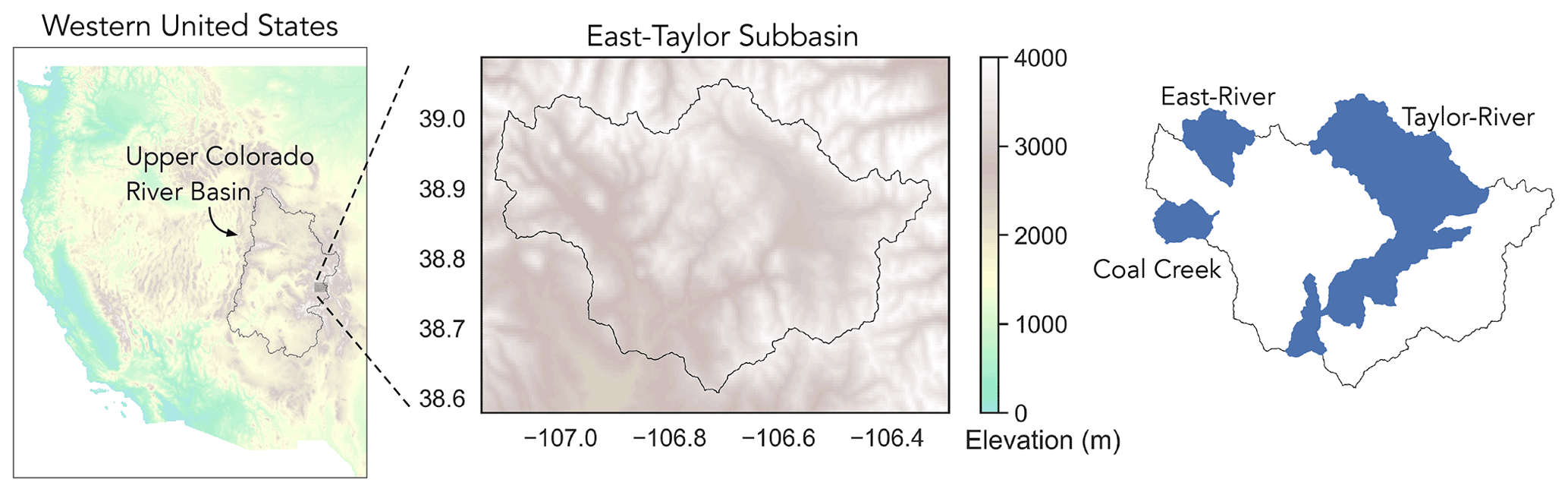
Figure 1Location of East–Taylor subbasin in the western United States. Also shown are several watersheds within East–Taylor that are subjected to research on water availability and quality.
2.1 Study area
Our study area is the East–Taylor subbasin (hydrologic unit code 14020001; Fig. 1), which is a mountainous watershed in Colorado, western United States. East–Taylor subbasin encompasses several watersheds including East River, Taylor River, and Coal Creek. These watersheds have been subjected to intensive research activity, some of which contain highly instrumented test beds developed for understanding the impact of watershed changes on water availability and quality (Hubbard et al., 2018). East–Taylor subbasin is also part of the Upper Colorado River basin (UCRB; hydrologic unit code 14), which is a site of the United States Geological Survey (USGS) Next Generation Water Observation System (NGWOS; Gallaudet and Petty, 2018). In general, UCRB is an important study area as it drains into the Colorado River which is the principal source of water and jobs for 40 million people in the southwestern United States and Mexico (James et al., 2014). The Colorado River is under increasing stress due to drought and changing seasonality of snowmelt (Milly and Dunne, 2020), which can significantly impact the regional economies. Generating hyper-resolution datasets of gridded meteorological forcing in UCRB can help with quantitative modeling efforts geared towards water security for the region.
We start with a relatively small study area within UCRB to make it easier to visualize and critically evaluate the datasets. The novelty of the downscaling methodology further motivates us to start with a smaller study area (i.e., East–Taylor subbasin) before expending resources to generate datasets that cover a larger area (i.e., UCRB and beyond). Since the East–Taylor subbasin is an area of intensive research activity, the generated datasets can be rapidly incorporated into land-surface and ecohydrological modeling. This will also help us to identify any missing features in the datasets which may drive further refinement of the underlying downscaling methodology (Sect. 3).
2.2 Data sources
2.2.1 Gridded meteorological data
We obtained gridded estimates of daily precipitation (which includes both rain and snow), maximum daily temperature, and minimum daily temperature from PRISM. The maximum and minimum values of temperature were averaged to obtain mean values of temperature. PRISM data at 800 m spatial resolution constitute a proprietary dataset purchased from the PRISM Climate Group at Oregon State University (https://prism.oregonstate.edu, last access: 6 August 2021). PRISM serves as the official spatial climate dataset of the United States Department of Agriculture (Daly et al., 2008). Its methodology (to account for orographic effects) and climatology have been leveraged to generate various gridded datasets (Livneh et al., 2013; Abatzoglou, 2013; Behnke et al., 2016; Xie et al., 2007; Xia et al., 2012).
2.2.2 Weather station data
We obtained daily weather station data from the Global Historical Climatology Network (GHCN; Menne et al., 2012). The GHCN-Daily dataset integrates daily climate observations from 80 000 stations worldwide and subjects them to a suite of quality assurance measures.
2.2.3 Elevation data
We obtained elevation maps from the National Elevation Dataset (NED; U.S. Geological Survey, 2019; https://apps.nationalmap.gov, last access: 30 July 2019) at a spatial resolution of 10 m.

Figure 2Lidar-derived SWE maps within the East–Taylor subbasin obtained via ASO: (a) spatial extent of the maps in East–Taylor and (b) actual maps (upscaled to 400 m resolution). Each map is labeled by its basin, date of acquisition, and fraction of snow-covered area (fSCA) at its native 50 m resolution. These maps constitute independent datasets that are not used for downscaling precipitation and temperature but for demonstrating an example use case (Sect. 6.1).
2.2.4 Lidar observations of snowpack
We obtained lidar maps of snow water equivalent (SWE) generated by the Airborne Snow Observatory (ASO) at a spatial resolution of 50 m (Painter, 2018). These maps constitute independent datasets that are used exclusively to demonstrate an example use case of the downscaled datasets and are not used in the downscaling methodology itself. Across the East–Taylor subbasin, the ASO data quantify SWE across Crested Butte (CB), Gunnison – East River (GE), and Gunnison – Taylor River (GT) basins (Fig. 2). There are eight maps across 2016 to 2019, out of which five correspond to the early-melt period (March/April), and three correspond to the late-melt period (May/June).
2.3 Data preprocessing
The above data streams (Sect. 2.2) were subjected to various preprocessing steps as described below.
2.3.1 Gridded meteorological data (PRISM)
PRISM defines a day as the 24 h period ending at noon UTC (Strachan and Daly, 2017). The time zone of our study area is UTC−07:00 (or UTC−06:00 during daylight savings) which means that, for a given day, the 24 h period ends at 05:00 local time (or 06:00 during daylight savings). We shifted the dates of the precipitation data backward by 1 d, so that the 24 h period starts (rather than ends) at 05:00 local time. A similar adjustment was made for dates of maximum daily temperature prior to computing values of mean daily temperature. The dates of minimum daily temperature were not changed since the minimum temperature is likely to occur early in the morning around or before 05:00 local time.
2.3.2 Weather station data
Weather station data were subjected to two steps of preprocessing. The first step addresses inconsistent reporting times. Some stations are automated and report observations that represent the 24 h period ending at midnight. However, most stations typically report daily observations at morning local time. The dates of precipitation and maximum temperature for the latter group of stations were shifted backward by 1 d, along the lines described for PRISM data above. Thornton et al. (2021) discuss this issue in more detail. The second step addresses gap-filling of missing values, which can happen for various reasons, such as equipment malfunction, network interruptions, and natural hazards. We gap-filled missing values of precipitation and mean temperature using a data-driven sequential imputation approach (Mital et al., 2020; Dwivedi et al., 2022). This approach helps to gap-fill missing values using neighboring weather stations. Importantly, this approach overcomes two key limitations of other imputation approaches, in that they do not require (i) specification of a functional form to do a weighted interpolation using neighboring weather stations and (ii) neighboring weather stations to have a complete time series. In particular, we used the approach detailed in Mital et al. (2020), which was developed specifically for meteorological variables.
2.3.3 Elevation data
Elevation maps were upscaled using bilinear interpolation (in increments of 2×), mosaicked and reprojected to align their grids with the PRISM data. This was done with the help of Python's Rasterio module (Gillies et al., 2013). The gridded elevation data were also used to derive gridded estimates of slope and aspect using Python's RichDEM module (Barnes, 2016).
2.3.4 Lidar observations of snowpack
The lidar maps were upscaled using bilinear interpolation (in maximum increments of 2×) and reprojected to align their grids with the PRISM data. The maps corresponding to Gunnison – East River (GE) required additional quality control measures (see Appendix A).
3.1 Data-driven model: random forests
We employ random forests (RFs) to implement our spatial downscaling methodology. RFs are a non-parametric machine learning method based on an ensemble of decision trees (Breiman, 2001). Decision trees seek to minimize the error in modeling the target variable by recursively partitioning the input feature (or predictor) space into smaller subspaces. For regression models, a typical error criterion is the mean-squared error. The RF model employs bootstrapping to generate a different set of data points for each decision tree. The final model output is obtained by mean aggregation of the output of all decision trees in the ensemble. RF models also provide measures of the relative “feature importance” of each predictor variable. We implemented RFs using Python's scikit-learn module (Pedregosa et al., 2011). The hyperparameter values employed in our RF models are specified in Appendix B.
3.2 Extracting relationships between topography, weather stations, and climate variables
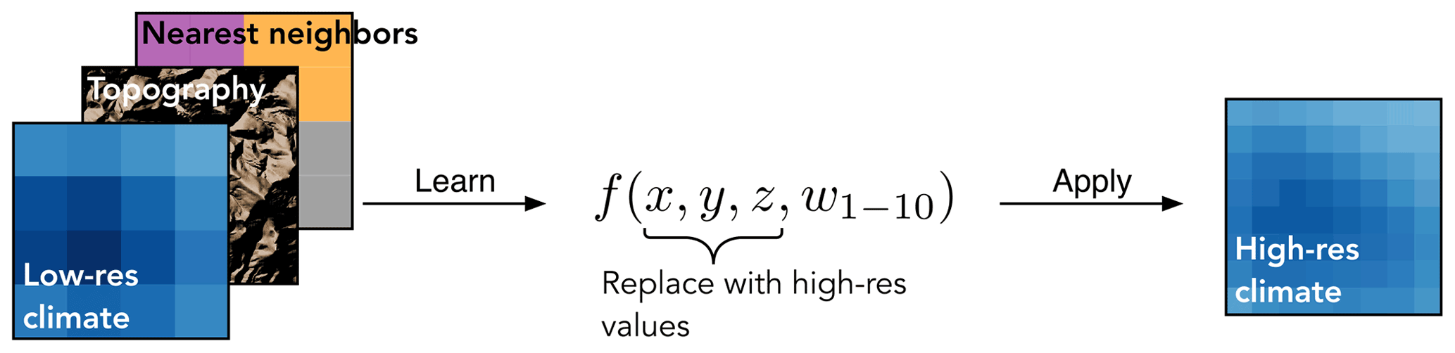
Our data-driven downscaling methodology consists of two steps: (i) learn the mapping between topographic features and the daily climate variable (at the native resolution of 800 m), and (ii) apply the learned mapping to model the downscaled climate variable using topographic features (at a resolution of 400 m). Figure 3 shows the schematic of the methodology. The gridded climate variable V can be expressed as the following function f:
where x, y, and z correspond to longitude, latitude, and elevation, respectively. These three spatial coordinates quantify the three-dimensional topography and enable the data-driven model to learn local relationships between V and physiography – relationships that correspond to expert knowledge embedded in the PRISM dataset. Finally, w1–10 corresponds to the 10 most correlated weather stations for each grid point. We use w1–10 as a shorthand notation for w1, w2, …, w10, where wi corresponds to the ith most correlated weather station for a grid point. w1–10 can be thought of as 10 nearest neighbors for each grid point. The PRISM dataset is developed using a weighted linear regression of weather station data. By using w1–10, we strive to give our machine learning model the same raw data that are used by the PRISM methodology. We picked 10 stations since it seems to correspond to the upper limit of the minimum number of stations that PRISM uses to develop a climate–elevation regression for a grid point (Daly et al., 1994). The use of w1–10 helps to constrain or regularize the relationship learned between the climate variable and topography, since it more explicitly forces the machine learning model to consider point measurement data. We determined w1–10 using the entire 12-year time series of the climate variable and weather stations. Figure 4 shows a map of w1. Note that since we are doing spatial downscaling, we learn the function f separately for each day. This also enabled us to get estimates of relative feature importance of each predictor variable, which are presented in Appendix C.
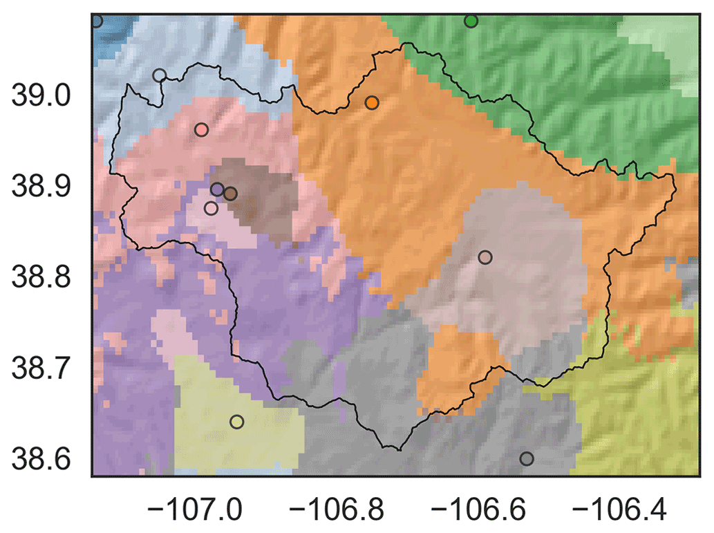
Figure 4First nearest-neighbor map (w1) of precipitation in the East–Taylor subbasin. Open circles correspond to locations of weather stations. Each grid point is color-coded using the color of its “first nearest-neighbor” weather station. Consequently, the map resembles a collection of polygons, where each polygon comprises grid points that have the same first nearest neighbor. Note that the first nearest neighbor for a grid point is not necessarily the closest station but the most correlated station. Some stations are outside the spatial extent of the map (not shown).
Finally, we subjected the downscaled precipitation grids to a variable filter as described by Daly et al. (2008). The filter performs a distance-weighted average of all surrounding grid cells and ensures a smooth precipitation field in low-gradient areas, without affecting the high-gradient areas.
We consider the following statistical measures (Sect. 4.1–4.4) to describe the downscaled datasets. Each measure helps focus on a salient feature of the datasets.
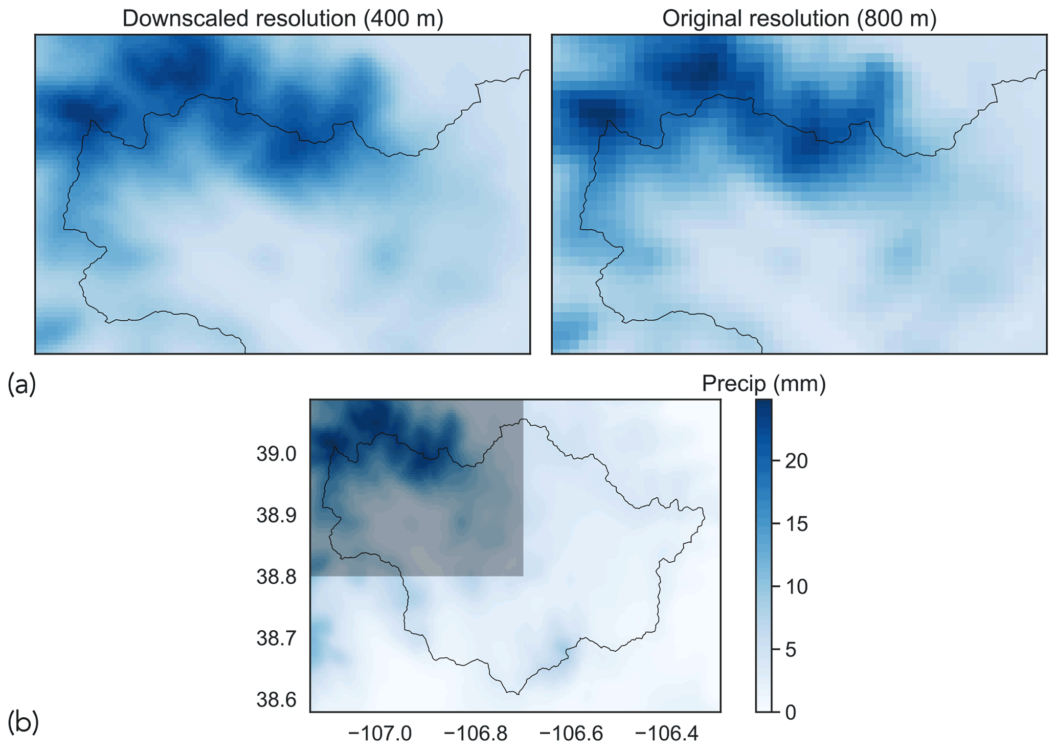
Figure 5Example of downscaled precipitation grid: (a) comparison of downscaled precipitation with original precipitation (date: 5 December 2019) and (b) gridded precipitation for the entire East–Taylor subbasin for the date in (a). The translucent box in the top left of (b) corresponds to the spatial extent shown in (a). The term “Precip” in the color bar is an abbreviation for precipitation.
4.1 Quantifying roughness
Gridded estimates of precipitation and temperature should exhibit a spatial variation that is consistent with the resolution of the grid. Projecting coarse-resolution meteorological variables on a fine-resolution grid results in discontinuous spatial gradients which can impact the modeling of land-surface processes (Maina et al., 2020). This implies that spatial gradients of the downscaled climate variables should exhibit a more gradual (or smoother) variation, when compared to their coarse-resolution counterparts. We explore the relative smoothness of the downscaled and original datasets by quantifying their roughness.
To quantify the roughness of a gridded climate variable, we start by computing its Laplacian. The Laplacian ℒ of a gridded variable is estimated by convolving the gridded variable with the following 3×3 filter:
The Laplacian can be used to visualize changes in gradients (or roughness) of the gridded variables. Its ability to capture the roughness of an image has long been utilized in computer vision for edge detection (Torre and Poggio, 1986). We estimate the roughness 𝒥 of a gridded variable by summing the element-wise squares of its Laplacian:
where ℒi,j corresponds to the (i,j)th element of ℒ. This approach to estimate roughness is motivated by the definition of roughness penalty used for fitting smooth splines to data (Gu, 2002). We expect the gridded variable at the downscaled resolution to have a lower roughness when compared to the original resolution. To compare the roughness at the two resolutions, we define a quantity called the roughness ratio (RR) as follows:
where the subscript corresponds to the spatial resolution of the gridded variable. RR <1 implies that 𝒥400<𝒥800, which means that the datasets are smoother at the downscaled resolution.
4.2 Quantifying spatial variability
In addition to exhibiting smooth spatial gradients, it is also important to check that the downscaled datasets preserve the spatial variability prevalent in the original datasets. We quantify the spatial variability of the climate variables by computing empirical semi-variograms using a discrete form of Matheron's estimator (Matheron, 1963):
where γ(h) refers to the semi-variogram, which is a function of distance or lag h, N(h) is the number of pairwise points for a given value of h, and Z(xi) is the value of a given field Z (here, precipitation or temperature) at location xi. If γ increases with h, it implies that the observed field Z is more dissimilar (or uncorrelated) at larger distances. We compute and compare the semi-variograms at both the downscaled and the original resolutions.
4.3 Quantifying residual error
The process of downscaling should not introduce any bias in the hyper-resolution datasets. We can verify this by upscaling the downscaled datasets back to the original resolution (i.e., 800 m) and quantifying the mean residual error with respect to the original datasets (also at 800 m resolution). For a given time point, we quantify the mean residual error R over the entire study area as follows:
where V refers to the value of the climate variable in the original dataset, refers to the upscaled value of the climate variable obtained from the downscaled dataset, the subscript j is the index of the grid point at the original resolution, and n is the total number of grid points in the dataset at the original resolution. The upscaling was done via bilinear interpolation. Ideally, the mean residual error should be close to zero, which implies that the downscaled datasets do not exhibit any bias when compared to the datasets at the original resolution.
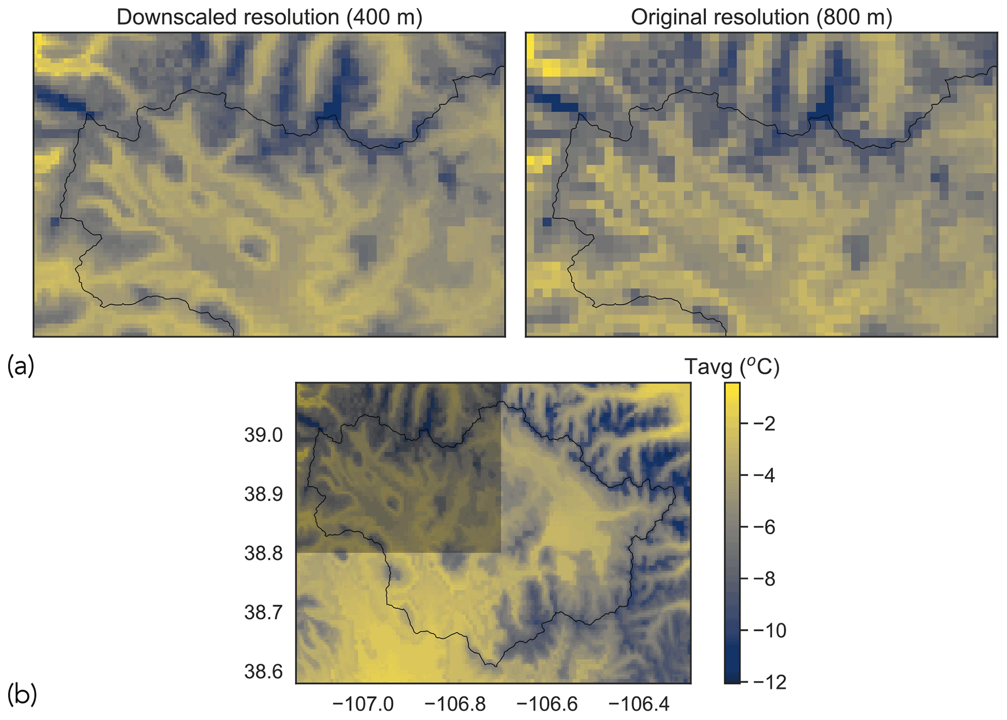
Figure 6Example of downscaled mean temperature grid: (a) comparison of downscaled temperature with original temperature (date: 5 December 2019) and (b) gridded mean temperature for the entire East–Taylor subbasin for the date in (a). The translucent box in the top left of (b) corresponds to the spatial extent shown in (a). The term “Tavg” in the color bar is an abbreviation for mean temperature.
4.4 Quantifying influence of elevation
PRISM assumes that for a localized region, elevation is the most important factor in the distribution of temperature and precipitation (Daly et al., 2008). Therefore, it is of interest to investigate how elevation influences the downscaled datasets. We do this using partial dependence plots (PDPs; Friedman, 2001), which show the marginal effect that a feature (here, elevation z) has on the outcome of a model. For regression, the partial dependence function is defined as (Molnar, 2019)
where z is the feature for which we obtain a PDP, and XC denotes the other features used in the machine learning model . Here, approximates the model f, as defined in Eq. (1), which is used to generate the downscaled datasets. The partial dependence function can be approximated using a Monte Carlo simulation whereby we consider all the instances of our data (which are used to learn ) and replace the true value of z with a realization of z instead. We can then obtain the average model prediction for each realization of z. We estimated the partial dependence functions for models used to generate downscale estimates of both precipitation and mean temperature.
While estimating roughness, mean residual error, and partial dependence (outlined in Eqs. 2, 4 and 5, respectively), we seek to visualize their spread rather than obtaining a single value. Therefore, we randomly sampled 100 time points (or days) and computed the above error metrics for each of those time points. This yields a sample size that is tractable and amenable to analysis and visualization while being large enough to yield a representative distribution. For precipitation, we considered only the wet days (when mean precipitation across East–Taylor was greater than 1 mm, which corresponds to the resolution of the weather station data). Dry days imply absence of precipitation, which precludes meaningful analysis. No such constraints on selection of days are needed for analyzing mean temperature.
5.1 Downscaled datasets exhibit smoother spatial gradients than their coarser counterparts
Figures 5 and 6 show examples of downscaled precipitation and mean temperature fields, along with their original counterparts. To visualize the differences, we have zoomed into the northwest extent of the basin as indicated in subfigures (b). The northwest extent of the basin encompasses the East River watershed, which is an area of sustained research activity (Hubbard et al., 2018). We note the prevalence of smoother spatial gradients at the downscaled resolution (400 m) when compared with the original resolution (800 m).

Figure 7Example of Laplacian of precipitation grid at the downscaled and original resolution for the date corresponding to Fig. 5. The color bar shows the Laplacian values (units of mm m−2).
We now quantify the smoothness (or roughness) of precipitation and temperature fields (as described in Sect. 4.1). Figure 7 shows an example of the Laplacian of precipitation at both the downscaled and original resolution, corresponding to the date shown in Fig. 5. For consistency, the precipitation at the original resolution has been projected to the downscaled grid. We note that the Laplacian for the downscaled precipitation varies smoothly. The Laplacian for precipitation at the original resolution is characterized by a checker-board pattern, which visualizes the need for generating hyper-resolution datasets while implementing hydrological models at hyper-resolutions.
Figure 8 shows the distributions of RRs for both precipitation and mean temperature. In both cases, the values of RR are well below 1, signifying that the spatial gradients of datasets are smoother at the downscaled resolution.
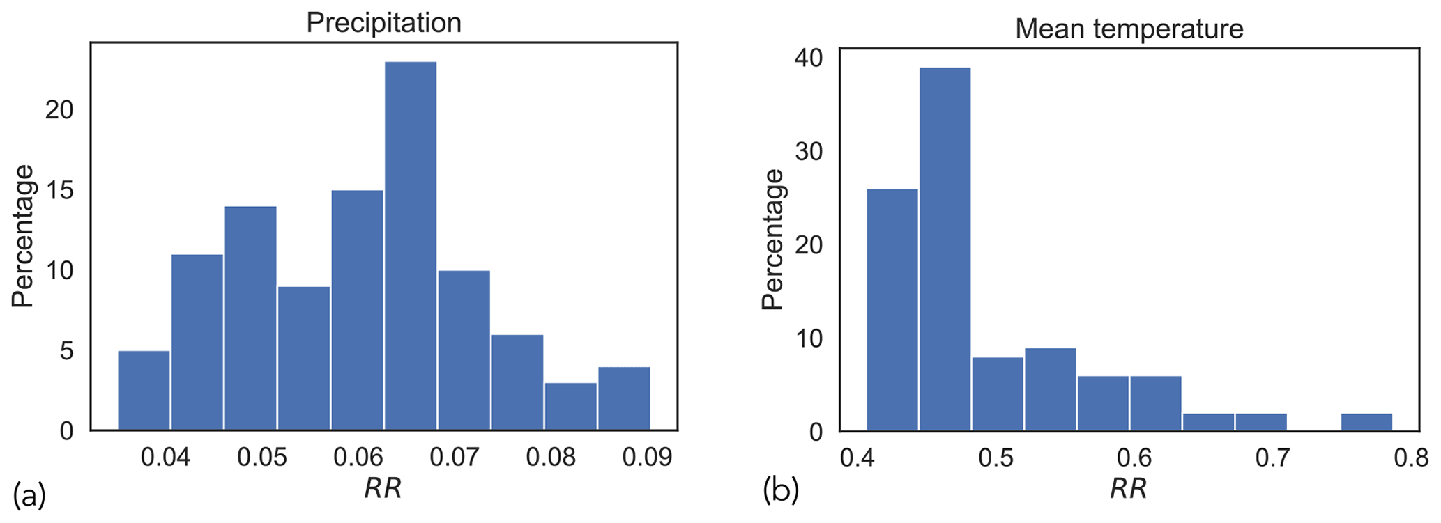
Figure 8Roughness ratio (RR) estimates for (a) precipitation and (b) mean temperature. RR is the ratio of downscaled roughness to original roughness shown in Eq. (2), where RR <1 implies that the datasets are smoother at the downscaled resolution.
5.2 Downscaled datasets preserve the spatial structure of the original datasets
Figure 9 shows examples of semi-variograms of precipitation and temperature fields. These examples correspond to the date in Figs. 5 and 6 (i.e., 5 December 2019). The variability at the downscaled resolution is similar to that at the original resolution. This shows that the downscaled datasets preserve the spatial structure of the climate field present in the original datasets.

Figure 9Semi-variograms for (a) precipitation and (b) mean temperature (date: 5 December 2019). The plots show that the downscaled datasets preserve the spatial structure of the climate field present in the original datasets.
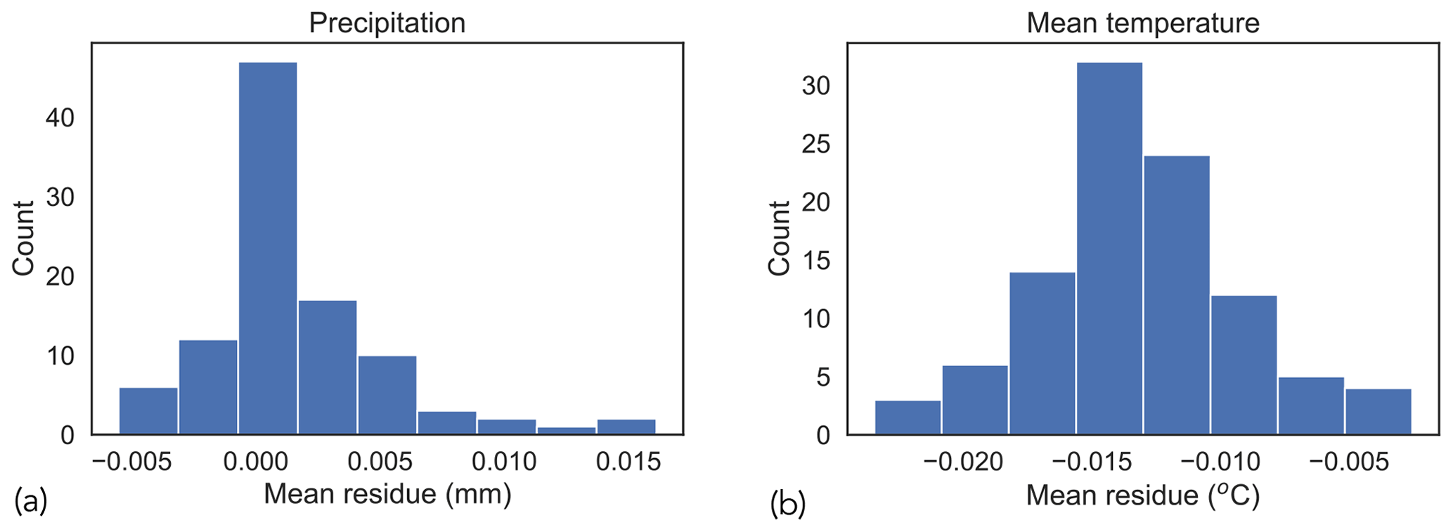
Figure 10Residual error of downscaled datasets for (a) precipitation and (b) mean temperature. The estimated value of mean residue for precipitation is 0.002 mm, with a standard error of 0.004 mm. The estimated value of mean residue for mean temperature is −0.01 ∘C, with a standard error of 0.004 ∘C.
5.3 Residual error of downscaled datasets
Figure 10 shows the distributions of mean residue (Sect. 4.3), where each instance corresponds to the mean residual error for a randomly selected time point. We clarify that “mean” in this context refers to the spatial mean over the entire study area. We observe that the estimated values of mean residue (as indicated by the peak value of the histogram) for both precipitation and mean temperature are close to zero. The small amount of residual error can be attributed to the fact that the downscaled dataset is generated using a machine learning model , which is an approximation of the true function f. Mean residual values of zero imply that the downscaled estimates do not exhibit any bias when compared with the dataset at the original resolution.
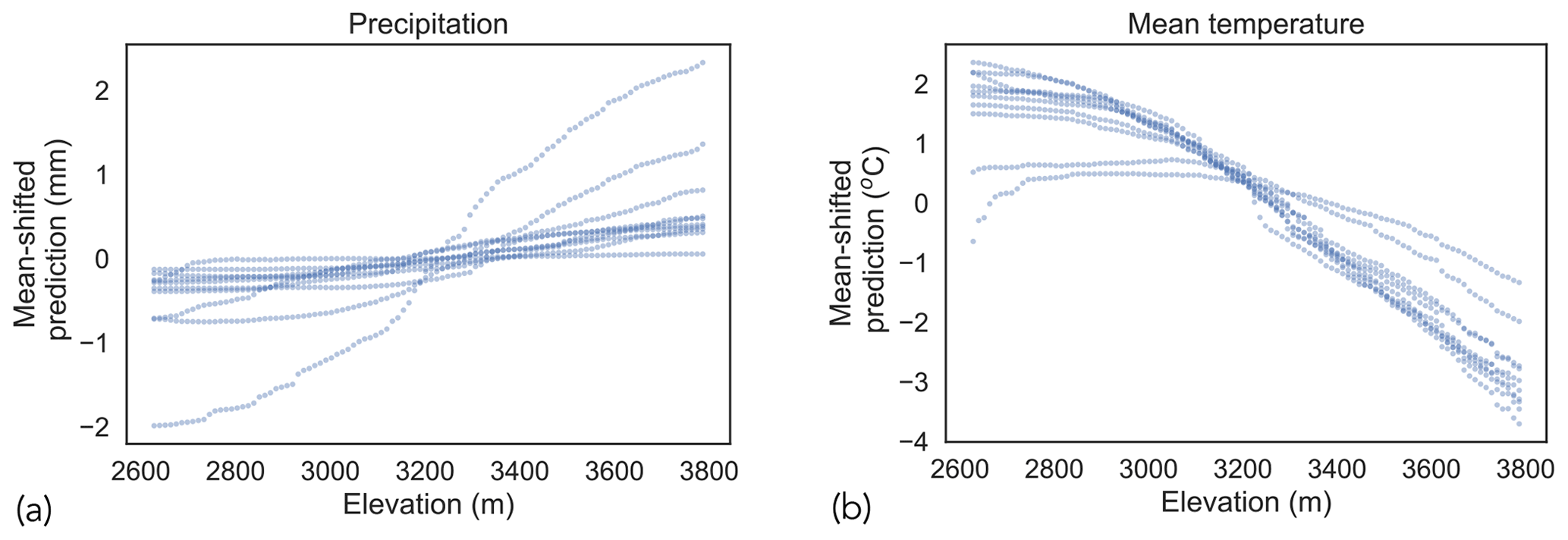
Figure 11Climate–elevation relationship visualized using PDPs for (a) precipitation and (b) mean temperature.
5.4 Effect of elevation on datasets
Figure 11 shows PDPs that marginalize the effect of elevation on each climate variable. For both climate variables, we show PDPs for 10 randomly selected days. Although PDPs were obtained for 100 d (as documented in the beginning of Sect. 5), we show results only for 10 d to prevent overcrowding of the plots. Furthermore, to enable visualization of multiple partial dependence functions on the same plot, we shifted each function by its mean value. The machine learning model used to generate downscaled datasets captures an increase (decrease) in precipitation (mean temperature) with increase in elevation, which is consistent with the local climatology and the PRISM datasets (Daly et al., 2008).
The downscaled datasets cannot be validated directly since the ground-truth climate field is not known. Instead, we present a use case to demonstrate that the downscaled datasets can be effective for ecohydrological modeling in complex mountainous terrains where climate gradients can change at fine spatial scales.
6.1 Modeling snowpack estimates
We developed a novel data-driven approach that models high-resolution SWE data obtained via lidar (as described in Sect. 2.2.4). Our feature space comprised several meteorological variables at downscaled (∼400 m) and original (∼800 m) resolutions. As part of the use case, we also evaluated if using downscaled meteorological variables can improve the modeling of SWE, when compared to using meteorological variables at original resolutions. Any improvement in snowpack (SWE) modeling can be considered a validation of the spatial patterns represented by the downscaled datasets. We provide a brief description of the four meteorological variables derived for this purpose, following Mital et al. (2022):
- i.
Accumulated snowfall. Snowfall is the primary mechanism behind snow accumulation. As snow accumulation takes place over the entire snow season, we consider accumulated snowfall from the start of the snow season (defined as 1 October) till the date of observation of the snowpack. Precipitation on a given day is considered to be snow if the mean air temperature is less than or equal to 0 ∘C.
- ii.
Positive degree-day sum (PDD sum). PDD sum is used to approximate the process of snowmelt and is defined as the sum of mean daily temperatures above 0 ∘C in a given time period. We consider PDD sum from the start of the snowmelt season (defined as 15 March).
- iii.
Accumulated precipitation. Since snowfall is extracted from precipitation using an approximate methodology, we also consider accumulated precipitation over the entire snow season.
- iv.
Mean seasonal air temperature (Tmean). Tmean is computed by averaging the mean daily temperatures from the start of the snow season (1 October) till the date of observation of the snowpack. This helps consider the spatial heterogeneity of temperature across a basin.
Note that the above variables are temporal aggregations, and as such the spatial structure of downscaled precipitation and temperature is preserved. In addition, we also considered the following five topographic variables: (v) elevation, (vi) slope, (vii) aspect, (viii) latitude, and (ix) longitude.
Figure 12 shows the schematic of the modeling approach, adapted from our previous work (Mital et al., 2022). We developed two RF models. RF model 1 used meteorological variables (i–iv) at the original (∼800 m) resolution, while RF model 2 used meteorological variables at the downscaled (∼400 m) resolution. Both models use topographic variables (v–ix) at the downscaled resolution. The target variable in both cases was SWE, also at the downscaled resolution. This enabled us to isolate the effect of using downscaled estimates of meteorological variables. The hyperparameter values for the RF models are specified in Appendix B.

Figure 12Feature space for the two RF models considered in our validation exercise. Meteorological variables refer to (i) accumulated snowfall, (ii) PDD sum, (iii) accumulated precipitation, and (iv) Tmean. Topographic variables refer to (v) elevation, (vi) slope, (vii) aspect, (viii) latitude, and (ix) longitude.

Figure 13Example use case of downscaled datasets showing scatter plots to predict SWE using RF model 2. The individual points are color-coded by elevation.
The RF models of spatially distributed SWE were evaluated using a leave-one-out approach. As described in Sect. 2.2.4, there are a total of eight distinct maps available within the study area. We trained each RF model using seven maps and evaluated their respective abilities to model the held-out map. This exercise was conducted eight times, where each time a different map was considered as a held-out map. We evaluated the model performance by computing the Nash–Sutcliffe efficiency (NSE; Nash and Sutcliffe, 1970) on the held-out map. NSE is defined as
where MSE is the mean-squared error of the model, and σo is the standard deviation of the observations in the held-out map. NSE is dimensionless, ranging from −∞ to 1. Higher values are desirable and are consistent with lower values of MSE.
Table 1Validation results of modeling SWE at 400 m. The resolution in parentheses refers to the resolution of meteorological variables. Both models used topographic variables at a resolution of 400 m. For each snapshot, higher NSE values are marked in bold.
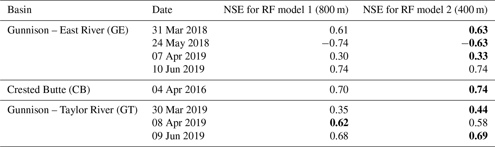
Table 1 shows the results of the modeling exercise, wherein we modeled SWE at 400 m resolution using both the original (RF model 1) and downscaled (RF model 2) meteorological variables. We observed that downscaled variables yield improvements (as indicated by higher NSE values) in six out of eight instances. The negative NSE values for GE: 24 May 2018 are due to that particular snapshot having the lowest fractional snow cover area compared to other snapshots (Fig. 2). This implies that the relationships between the predictors and SWE are different when compared to other snapshots (Mital et al., 2022). Overall, the results in Table 1 suggest that even if the downscaled dataset may not capture all the spatial variability at hyper-resolutions, it still constitutes a superior product compared to the original dataset especially when it comes to modeling hydrological variables at hyper-resolutions. Figure 13 shows scatter plots between the observed and predicted (modeled) SWE using RF model 2.
6.2 Additional use cases: impact of meteorological forcing resolution on hydrological responses
Additional use cases of downscaled datasets involve studies that investigate the impact of spatial and temporal resolution of gridded meteorological forcing on watershed hydrological responses (Shuai et al., 2022; Maina et al., 2020). For instance, Shuai et al. (2022) explored the effects of spatial and temporal resolution of gridded meteorological forcing on watershed hydrological responses. The study used integrated hydrological modeling and was conducted in the Coal Creek watershed, which is a mountainous sub-watershed located at the western edge of the East–Taylor subbasin. The downscaled daily datasets were used as high-resolution forcing variables, and the simulated streamflow was found to be consistent when compared with the results of coarser-resolution forcings. The study also considered a number of additional hydrological variables (i.e., SWE, snowmelt, ponded depth, groundwater level, soil moisture, and evapotranspiration). For more details, we refer the reader to Shuai et al. (2022).
The use cases presented and reviewed in this study evaluated the impact of using downscaled meteorological variables for modeling the hydrological response in mountainous regions. As the presented use case modeled snowpack using a data-driven framework, it is possible that not all the factors driving spatial variability of snowpack were considered. Additional evaluation of downscaled datasets may require access to spatially distributed ground-truth data at hyper-resolutions (e.g., via X-band radar), as well as comparisons with hyper-resolutions outputs (if available) of land-surface and numerical weather prediction models. Future work will expand the study area to a larger spatial extent (i.e., UCRB and beyond).
It is important to note that a lack of hyper-resolution observations makes it challenging to estimate the true errors associated with gridded datasets (Daly, 2006). Nevertheless, it is important to pursue development of hyper-resolution datasets (such as the ones presented in this study) so that they can be visualized and critically evaluated (Beven et al., 2015). This enables identification of any missing features and drives further refinement of methodologies for generating hyper-resolution datasets. Additional research is needed to reliably downscale gridded datasets to finer resolutions (i.e., beyond 400 m), and it may require us to consider additional information (e.g., canopy, multispectral satellite data, radar data).
The presented dataset is freely available on the United States Department of Energy's Environmental System Science Data Infrastructure for a Virtual Ecosystem (ESS-DIVE) repository. It can be accessed at https://doi.org/10.15485/1822259 and cited as Mital et al. (2021). We recommend accessing the dataset using Chrome or Firefox browsers. The dataset consists of two zip files: one for daily precipitation and one for daily mean temperature. The data are arranged by year and are in the NetCDF format, which is a standard raster format that can be read using Geographic Information System software and popular scripting languages (e.g, R, Python, MATLAB). The datasets have been projected to the coordinate system denoted by NAD83/UTM zone 13N – EPSG:26913. A Jupyter notebook has been provided in the Supplement which illustrates the spatial downscaling methodology.
We have presented a description of a hyper-resolution (400 m) gridded dataset of daily precipitation and mean temperature. The datasets cover a 12-year period of 2008–2019. The spatial extent of the datasets is the East–Taylor subbasin, which is a mountainous watershed and is an important study area in the context of water security for the southwestern United States and Mexico (Sect. 2.1). The datasets were generated by downscaling daily gridded datasets developed by the PRISM group (800 m resolution). Rather than seeking to train on paired coarse-resolution and fine-resolution data (which are not available), our methodology sought to learn relationships between topographic features and daily climate variables. These relationships were constrained or regularized by the use of nearest-neighbor maps that forced the machine learning model to more explicitly consider point observations. The relationships were then implemented to generate downscaled datasets. Downscaling enabled us to leverage knowledge about physiographic factors and climatological processes that are embedded in the existing datasets.
The precipitation and temperature fields at the downscaled resolution provide a more precise definition of local gradients (and preserve the spatial variability) when compared with the original dataset. This can aid in the implementation of hydrological and land-surface models in complex mountainous terrains with fine-scale spatial gradients. The downscaled fields also do not exhibit any bias when compared with the original dataset, as demonstrated by a mean residual error that is approximately zero. We observe the prevalence of linear relationships between climate variables and elevation, which is consistent with the PRISM datasets. Finally, we demonstrated a use case for downscaled datasets by implementing a data-driven framework to model snowpack. The presented dataset constitutes a valuable resource to implement ecohydrological and land-surface models in the mountainous terrain of the East–Taylor subbasin.
The lidar maps corresponding to Gunnison – East River (GE) required additional quality control measures. First, a number of pixels in the GE maps appeared to be numerical artifacts. To remove these artifacts, we assumed that the map labeled GE: 31 March 2018 recorded a continuous snow cover (given that the date is close to peak SWE; Clow, 2010) Therefore, any pixels with SWE ≤0 were masked. The unmasked pixels gave us an initial spatial extent for GE maps. However, this initial spatial extent exceeded the spatial extent for the map labeled GE: 10 June 2019. Therefore, we considered an intersection of the two spatial extents, which yielded a consistent spatial extent across all four GE maps. This spatial extent is shown in Fig. 2b. Subsequently, we cropped part of the GE maps that fell outside the East–Taylor subbasin, yielding a final spatial extent as shown in Fig. 2a.
We used RF to learn the function f for spatial downscaling, as well for modeling snowpack in our example use case. Concerning the choice of hyperparameters for both sets of RF models, we sought to use values that were specified as default choices by the developers of RF (as documented at https://CRAN.R-project.org/package=randomForest, last access: 6 August 2021). Therefore, we specified 500 trees, considered features when looking for the best split (where p is the number of predictor variables), and specified a node size (i.e., minimum number of samples in a leaf node) of 5. For spatial downscaling, we specified a node size of 1 (instead of 5) to encourage growth of deep trees. The use of nearest neighbors (i.e, w1–10) as predictors helped alleviate any overfitting that may happen with deep trees. Note that the number of predictor variables (i.e, p) is 13 for spatial downscaling and 9 for the use case.
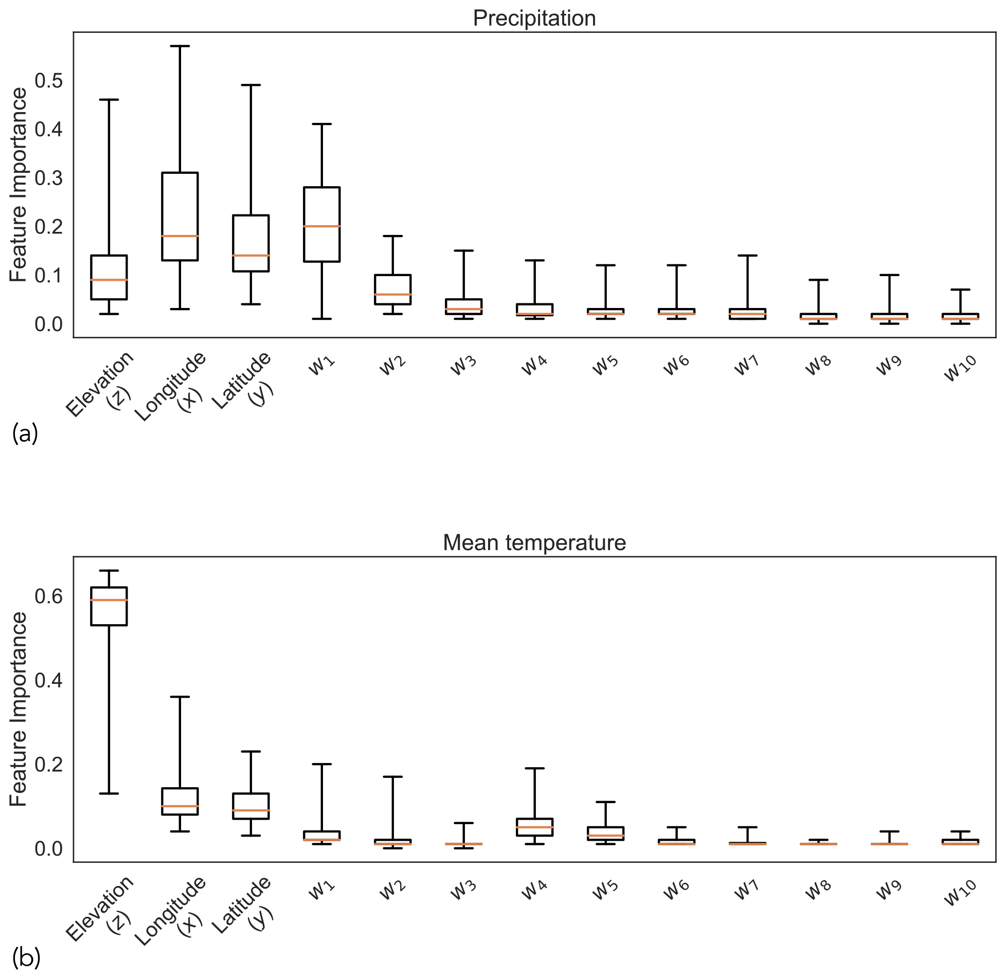
Figure C1 shows estimates of feature importance of RF models trained to downscale precipitation and mean temperature. For precipitation, we observe that all three topographic variables (i.e., elevation, longitude, latitude) along with the first two nearest neighbors (i.e., w1 and w2) are important for model predictions. For mean temperature, elevation has an outsized influence, with nearest neighbors having very little impact on the model predictions. Daily precipitation exhibits high spatial variability, which is not necessarily a function of changes in local topography (e.g., rain shadow effect, seeder-feeder mechanisms), making it important to explicitly consider information from nearby weather stations. The variability of mean daily temperature is more closely related to changes in elevation on account of the adiabatic lapse rate. As a result, there is a lower dependence on other factors.
The supplement related to this article is available online at: https://doi.org/10.5194/essd-14-4949-2022-supplement.
UM and DD conceived the study. UM curated the data, developed and implemented the downscaling methodology, and verified and validated the generated datasets. DD and JBB provided input on the overall methodology. CIS provided input on the conception of the study, provided overall supervision, and acquired funding for the study. UM prepared the manuscript with contributions from all co-authors.
The contact author has declared that none of the authors has any competing interests.
Publisher's note: Copernicus Publications remains neutral with regard to jurisdictional claims in published maps and institutional affiliations.
This work was funded by the ExaSheds project, which was supported by the U.S. Department of Energy, Office of Science, Office of Biological and Environmental Research, Earth and Environmental Systems Sciences Division, Data Management Program, under award no. DE-AC02-05CH11231. The proprietary PRISM data (800 m resolution) were purchased with funding from the Watershed Function Scientific Focus Area funded by the U.S. Department of Energy, Office of Science, Office of Biological and Environmental Research under award no. DE-AC02-05CH11231.
This paper was edited by Conrad Jackisch and reviewed by two anonymous referees.
Abatzoglou, J. T.: Development of gridded surface meteorological data for ecological applications and modelling, Int. J. Climatol., 33, 121–131, https://doi.org/10.1002/joc.3413, 2013.
Baño-Medina, J., Manzanas, R., and Gutiérrez, J. M.: Configuration and intercomparison of deep learning neural models for statistical downscaling, Geosci. Model Dev., 13, 2109–2124, https://doi.org/10.5194/gmd-13-2109-2020, 2020.
Barnes, R.: RichDEM: Terrain Analysis Software, gitHub [software], http://github.com/r-barnes/richdem (last access: 15 January 2022), 2016.
Behnke, R., Vavrus, S., Allstadt, A., Albright, T., Thogmartin, W. E., and Radeloff, V. C.: Evaluation of downscaled, gridded climate data for the conterminous United States, Ecol. Appl., 26, 1338–1351, https://doi.org/10.1002/15-1061, 2016.
Beven, K., Cloke, H., Pappenberger, F., Lamb, R., and Hunter, N.: Hyperresolution information and hyperresolution ignorance in modelling the hydrology of the land surface, Sci. China Earth Sci., 58, 25–35, https://doi.org/10.1007/s11430-014-5003-4, 2015.
Bierkens, M. F. P.: Global hydrology 2015: State, trends, and directions, Water Resour. Res., 51, 4923–4947, https://doi.org/10.1002/2015WR017173, 2015.
Breiman, L.: Random Forests, Mach. Learn., 45, 5–32, https://doi.org/10.1023/A:1010933404324, 2001.
Bürger, G., Murdock, T. Q., Werner, A. T., Sobie, S. R., and Cannon, A. J.: Downscaling Extremes–An Intercomparison of Multiple Statistical Methods for Present Climate, J. Climate, 25, 4366–4388, https://doi.org/10.1175/JCLI-D-11-00408.1, 2012.
Clow, D. W.: Changes in the Timing of Snowmelt and Streamflow in Colorado: A Response to Recent Warming, J. Climate, 23, 2293–2306, https://doi.org/10.1175/2009JCLI2951.1, 2010.
Cotter, A. S., Chaubey, I., Costello, T. A., Soerens, T. S., and Nelson, M. A.: Water quality model output uncertainty as affected by spatial resolution of input data, J. Am. Water Resour. As., 39, 977–986, https://doi.org/10.1111/j.1752-1688.2003.tb04420.x, 2003.
Coulibaly, P., Dibike, Y. B., and Anctil, F.: Downscaling Precipitation and Temperature with Temporal Neural Networks, J. Hydrometeorol., 6, 483–496, https://doi.org/10.1175/JHM409.1, 2005.
Crespi, A., Matiu, M., Bertoldi, G., Petitta, M., and Zebisch, M.: A high-resolution gridded dataset of daily temperature and precipitation records (1980–2018) for Trentino-South Tyrol (north-eastern Italian Alps), Earth Syst. Sci. Data, 13, 2801–2818, https://doi.org/10.5194/essd-13-2801-2021, 2021.
Daly, C.: Guidelines for assessing the suitability of spatial climate data sets, Int. J. Climatol., 26, 707–721, https://doi.org/10.1002/joc.1322, 2006.
Daly, C., Neilson, R. P., and Phillips, D. L.: A Statistical-Topographic Model for Mapping Climatological Precipitation over Mountainous Terrain, J. Appl. Meteorol., 33, 140–158, https://doi.org/10.1175/1520-0450(1994)033<0140:ASTMFM>2.0.CO;2, 1994.
Daly, C., Halbleib, M., Smith, J. I., Gibson, W. P., Doggett, M. K., Taylor, G. H., Curtis, J., and Pasteris, P. P.: Physiographically sensitive mapping of climatological temperature and precipitation across the conterminous United States, Int. J. Climatol., 28, 2031–2064, https://doi.org/10.1002/joc.1688, 2008.
Dwivedi, D., Mital, U., Faybishenko, B., Dafflon, B., Varadharajan, C., Agarwal, D., Williams, K. H., Steefel, C., and Hubbard, S.: Imputation of Contiguous Gaps and Extremes of Subhourly Groundwater Time Series Using Random Forests, J. Mach. Learn. Model Comput., 3, 1–22, https://doi.org/10.1615/JMachLearnModelComput.2021038774, 2022.
Feldman, D., Aiken, A., Boos, W., Carroll, R., Chandrasekar, V., Collins, W., Collis, S., Deems, J., DeMott, P., Fan, J., Flores, A., Gochis, D., Harrington, J., Kumjian, M., Leung, L., O'Brien, T., Raleigh, M., Rhoades, A., McKenzie Skiles, S., Smith, J., Sullivan, R., Ullrich, P., Varble, A., and Williams, K.: Surface Atmosphere Integrated Field Laboratory (SAIL) Science Plan, Technical Report, https://doi.org/10.2172/1781024, 2021.
Fiddes, J. and Gruber, S.: TopoSCALE v.1.0: downscaling gridded climate data in complex terrain, Geosci. Model Dev., 7, 387–405, https://doi.org/10.5194/gmd-7-387-2014, 2014.
Friedman, J. H.: Greedy Function Approximation: A Gradient Boosting Machine, Ann. Stat., 29, 1189–1232, 2001.
Gallaudet, T. and Petty, T. R.: Federal action plan for improving forecasts of water availability: Prepared pursuant to Section 3 of the October 19, 2018 Presidential Memorandum on Promoting the Reliable Supply and Delivery of Water in the West, https://d9-wret.s3.us-west-2.amazonaws.com/assets/palladium/production/s3fs-public/atoms/files/UCOL-BriefingSheet final.pdf (last access: 6 November 2021), 2018.
Gillies, S. and others: Rasterio: geospatial raster I/O for Python programmers, GitHub [code], https://github.com/rasterio/rasterio (last access: 15 January 2022), 2013.
Giorgi, F.: Thirty Years of Regional Climate Modeling: Where Are We and Where Are We Going next?, J. Geophys. Res.-Atmos., 124, 5696–5723, https://doi.org/10.1029/2018JD030094, 2019.
Groenke, B., Madaus, L., and Monteleoni, C.: ClimAlign: Unsupervised statistical downscaling of climate variables via normalizing flows, in: Proceedings of the 10th International Conference on Climate Informatics, CI2020, United Kingdom (virtual), 22–25 September 2020, 60–66, https://doi.org/10.1145/3429309.3429318, 2020.
Gu, C.: Smoothing spline ANOVA models, Springer, New York, London, https://doi.org/10.1007/978-1-4757-3683-0, 2002.
Gutiérrez, J. M., Maraun, D., Widmann, M., Huth, R., Hertig, E., Benestad, R., Roessler, O., Wibig, J., Wilcke, R., Kotlarski, S., San Martín, D., Herrera, S., Bedia, J., Casanueva, A., Manzanas, R., Iturbide, M., Vrac, M., Dubrovsky, M., Ribalaygua, J., Pórtoles, J., Räty, O., Räisänen, J., Hingray, B., Raynaud, D., Casado, M. J., Ramos, P., Zerenner, T., Turco, M., Bosshard, T., Štěpánek, P., Bartholy, J., Pongracz, R., Keller, D. E., Fischer, A. M., Cardoso, R. M., Soares, P. M. M., Czernecki, B., and Pagé, C.: An intercomparison of a large ensemble of statistical downscaling methods over Europe: Results from the VALUE perfect predictor cross-validation experiment, Int. J. Climatol., 39, 3750–3785, https://doi.org/10.1002/joc.5462, 2019.
Haylock, M. R., Hofstra, N., Klein Tank, A. M. G., Klok, E. J., Jones, P. D., and New, M.: A European daily high-resolution gridded data set of surface temperature and precipitation for 1950–2006, J. Geophys. Res.-Atmos., 113, D20119, https://doi.org/10.1029/2008JD010201, 2008.
Hubbard, S. S., Williams, K. H., Agarwal, D., Banfield, J., Beller, H., Bouskill, N., Brodie, E., Carroll, R., Dafflon, B., Dwivedi, D., Falco, N., Faybishenko, B., Maxwell, R., Nico, P., Steefel, C., Steltzer, H., Tokunaga, T., Tran, P. A., Wainwright, H., and Varadharajan, C.: The East River, Colorado, Watershed: A Mountainous Community Testbed for Improving Predictive Understanding of Multiscale Hydrological–Biogeochemical Dynamics, Vadose Zone J., 17, 1–25, https://doi.org/10.2136/vzj2018.03.0061, 2018.
James, T., Evans, A., Madly, E., and Kelly, C.: The economic importance of the Colorado River to the basin region, L William Seidman Research Institute, W. P. Carey School of Business, Arizona State University, https://businessforwater.org/wp-content/uploads/2016/12/PTF-Final-121814.pdf (last access: 4 February 2021), 2014.
Kunkel, K. E.: Simple Procedures for Extrapolation of Humidity Variables in the Mountainous Western United States, J. Climate, 2, 656–670, https://doi.org/10.1175/1520-0442(1989)002<0656:SPFEOH>2.0.CO;2, 1989.
Liston, G. E. and Elder, K.: A Meteorological Distribution System for High-Resolution Terrestrial Modeling (MicroMet), J. Hydrometeorol., 7, 217–234, https://doi.org/10.1175/JHM486.1, 2006.
Liu, Y., Ganguly, A. R., and Dy, J.: Climate Downscaling Using YNet: A Deep Convolutional Network with Skip Connections and Fusion, in: Proceedings of the 26th ACM SIGKDD International Conference on Knowledge Discovery & Data Mining, KDD '20: The 26th ACM SIGKDD Conference on Knowledge Discovery and Data Mining, Virtual Event CA USA, 6–10 July 2020, 3145–3153, https://doi.org/10.1145/3394486.3403366, 2020.
Livneh, B., Rosenberg, E. A., Lin, C., Nijssen, B., Mishra, V., Andreadis, K. M., Maurer, E. P., and Lettenmaier, D. P.: A Long-Term Hydrologically Based Dataset of Land Surface Fluxes and States for the Conterminous United States: Update and Extensions, J. Climate, 26, 9384–9392, https://doi.org/10.1175/JCLI-D-12-00508.1, 2013.
Lussana, C., Tveito, O. E., Dobler, A., and Tunheim, K.: seNorge_2018, daily precipitation, and temperature datasets over Norway, Earth Syst. Sci. Data, 11, 1531–1551, https://doi.org/10.5194/essd-11-1531-2019, 2019.
Maina, F. Z., Siirila-Woodburn, E. R., and Vahmani, P.: Sensitivity of meteorological-forcing resolution on hydrologic variables, Hydrol. Earth Syst. Sci., 24, 3451–3474, https://doi.org/10.5194/hess-24-3451-2020, 2020.
Matheron, G.: Principles of geostatistics, Econ. Geol., 58, 1246–1266, https://doi.org/10.2113/gsecongeo.58.8.1246, 1963.
Menne, M. J., Durre, I., Vose, R. S., Gleason, B. E., and Houston, T. G.: An Overview of the Global Historical Climatology Network-Daily Database, J. Atmos. Ocean. Tech., 29, 897–910, https://doi.org/10.1175/JTECH-D-11-00103.1, 2012.
Milly, P. C. D. and Dunne, K. A.: Colorado River flow dwindles as warming-driven loss of reflective snow energizes evaporation, Science, 367, 1252–1255, https://doi.org/10.1126/science.aay9187, 2020.
Misra, S., Sarkar, S., and Mitra, P.: Statistical downscaling of precipitation using long short-term memory recurrent neural networks, Theor. Appl. Climatol., 134, 1179–1196, https://doi.org/10.1007/s00704-017-2307-2, 2018.
Mital, U., Dwivedi, D., Brown, J. B., Faybishenko, B., Painter, S. L., and Steefel, C. I.: Sequential Imputation of Missing Spatio-Temporal Precipitation Data Using Random Forests, Front. Water, 2, 20, https://doi.org/10.3389/frwa.2020.00020, 2020.
Mital, U., Dwivedi, D., Brown, J. B., and Steefel, C. I.: Downscaled precipitation and mean air temperature datasets; East-Taylor subbasin; 2008–2019; daily temporal resolution; 400 m spatial resolution, ESS-DIVE [data set], https://doi.org/10.15485/1822259, 2021.
Mital, U., Dwivedi, D., Özgen-Xian, I., Brown, J. B., and Steefel, C. I.: Modeling Spatial Distribution of Snow Water Equivalent by Combining Meteorological and Satellite Data with Lidar Maps, Artificial Intelligence for the Earth Systems, early online release, https://doi.org/10.1175/AIES-D-22-0010.1, 2022.
Molnar, C.: Interpretable Machine Learning: A Guide for Making Black Box Models Explainable, 2nd edn., https://christophm.github.io/interpretable-ml-book (last access: 4 January 2022), 2019.
Mott, R., Vionnet, V., and Grünewald, T.: The Seasonal Snow Cover Dynamics: Review on Wind-Driven Coupling Processes, Front. Earth Sci., 6, 197, https://doi.org/10.3389/feart.2018.00197, 2018.
Mouatadid, S., Easterbrook, S., and Erler, A. R.: A Machine Learning Approach to Non-uniform Spatial Downscaling of Climate Variables, in: 2017 IEEE International Conference on Data Mining Workshops (ICDMW), 2017 IEEE International Conference on Data Mining Workshops (ICDMW), New Orleans, LA, 18–21 November 2017, 332–341, https://doi.org/10.1109/ICDMW.2017.49, 2017.
Nash, J. E. and Sutcliffe, J. V.: River flow forecasting through conceptual models part I – A discussion of principles, J. Hydrol., 10, 282–290, https://doi.org/10.1016/0022-1694(70)90255-6, 1970.
National Research Council: New Strategies for America's Watersheds, National Academies Press, Washington, D.C., https://doi.org/10.17226/6020, 1999.
Nourani, V., Razzaghzadeh, Z., Baghanam, A. H., and Molajou, A.: ANN-based statistical downscaling of climatic parameters using decision tree predictor screening method, Theor. Appl. Climatol., 137, 1729–1746, https://doi.org/10.1007/s00704-018-2686-z, 2019.
Painter, T. H.: ASO L4 Lidar Snow Water Equivalent 50m UTM Grid, Version 1, NASA National Snow and Ice Data Center Distributed Active Archive Center [data set], https://doi.org/10.5067/M4TUH28NHL4Z, 2018.
Pedregosa, F., Varoquaux, G., Gramfort, A., Michel, V., Thirion, B., Grisel, O., Blondel, M., Prettenhofer, P., Weiss, R., Dubourg, V., Vanderplas, J., Passos, A., and Cournapeau, D.: Scikit-learn: Machine Learning in Python, J. Mach. Learn. Res., 12, 2825–2830, 2011.
Rouf, T., Mei, Y., Maggioni, V., Houser, P., and Noonan, M.: A Physically Based Atmospheric Variables Downscaling Technique, J. Hydrometeorol., 21, 93–108, https://doi.org/10.1175/JHM-D-19-0109.1, 2020.
Sachindra, D. A., Ahmed, K., Rashid, Md. M., Shahid, S., and Perera, B. J. C.: Statistical downscaling of precipitation using machine learning techniques, Atmos. Res., 212, 240–258, https://doi.org/10.1016/j.atmosres.2018.05.022, 2018.
Sen Gupta, A. and Tarboton, D. G.: A tool for downscaling weather data from large-grid reanalysis products to finer spatial scales for distributed hydrological applications, Environ. Modell. Softw., 84, 50–69, https://doi.org/10.1016/j.envsoft.2016.06.014, 2016.
Shuai, P., Chen, X., Mital, U., Coon, E. T., and Dwivedi, D.: The effects of spatial and temporal resolution of gridded meteorological forcing on watershed hydrological responses, Hydrol. Earth Syst. Sci., 26, 2245–2276, https://doi.org/10.5194/hess-26-2245-2022, 2022.
Singh, V. P.: Effect of spatial and temporal variability in rainfall and watershed characteristics on stream flow hydrograph, Hydrol. Process., 11, 1649–1669, https://doi.org/10.1002/(SICI)1099-1085(19971015)11:12<1649::AID-HYP495>3.0.CO;2-1, 1997.
Škrk, N., Serrano-Notivoli, R., Čufar, K., Merela, M., Črepinšek, Z., Kajfež Bogataj, L., and de Luis, M.: SLOCLIM: a high-resolution daily gridded precipitation and temperature dataset for Slovenia, Earth Syst. Sci. Data, 13, 3577–3592, https://doi.org/10.5194/essd-13-3577-2021, 2021.
Strachan, S. and Daly, C.: Testing the daily PRISM air temperature model on semiarid mountain slopes, J. Geophys. Res.-Atmos., 122, 5697–5715, https://doi.org/10.1002/2016JD025920, 2017.
Tapiador, F. J., Navarro, A., Moreno, R., Sánchez, J. L., and García-Ortega, E.: Regional climate models: 30 years of dynamical downscaling, Atmos. Res., 235, 104785, https://doi.org/10.1016/j.atmosres.2019.104785, 2020.
Thornton, M. M., Shrestha, R., Wei, Y., Thornton, P. E., and Wilson, B. E.: Daymet: Daily Surface Weather Data on a 1-km Grid for North America, Version 4, ORNL DAAC [data set], https://doi.org/10.3334/ORNLDAAC/1840, 2020.
Thornton, P. E., Shrestha, R., Thornton, M., Kao, S.-C., Wei, Y., and Wilson, B. E.: Gridded daily weather data for North America with comprehensive uncertainty quantification, Sci. Data, 8, 190, https://doi.org/10.1038/s41597-021-00973-0, 2021.
Torre, V. and Poggio, T. A.: On Edge Detection, IEEE T. Pattern Anal., PAMI-8, 147–163, https://doi.org/10.1109/TPAMI.1986.4767769, 1986.
U.S. Geological Survey: The National Map–New data delivery homepage, advanced viewer, lidar visualization, Reston, VA, https://doi.org/10.3133/fs20193032, 2019.
Vandal, T., Kodra, E., Ganguly, S., Michaelis, A., Nemani, R., and Ganguly, A. R.: DeepSD: Generating High Resolution Climate Change Projections through Single Image Super-Resolution, in: Proceedings of the 23rd ACM SIGKDD International Conference on Knowledge Discovery and Data Mining – KDD '17, the 23rd ACM SIGKDD International Conference, Halifax, NS, Canada, 13–17 August 2017, 1663–1672, https://doi.org/10.1145/3097983.3098004, 2017.
Vandal, T., Kodra, E., and Ganguly, A. R.: Intercomparison of machine learning methods for statistical downscaling: the case of daily and extreme precipitation, Theor. Appl. Climatol., 137, 557–570, https://doi.org/10.1007/s00704-018-2613-3, 2019.
Vörösmarty, C. J., McIntyre, P. B., Gessner, M. O., Dudgeon, D., Prusevich, A., Green, P., Glidden, S., Bunn, S. E., Sullivan, C. A., Liermann, C. R., and Davies, P. M.: Global threats to human water security and river biodiversity, Nature, 467, 555–561, https://doi.org/10.1038/nature09440, 2010.
Xia, Y., Mitchell, K., Ek, M., Cosgrove, B., Sheffield, J., Luo, L., Alonge, C., Wei, H., Meng, J., Livneh, B., Duan, Q., and Lohmann, D.: Continental-scale water and energy flux analysis and validation for North American Land Data Assimilation System project phase 2 (NLDAS-2): 2. Validation of model-simulated streamflow, J. Geophys. Res.-Atmos., 117, D3110, https://doi.org/10.1029/2011JD016051, 2012.
Xie, P., Chen, M., Yang, S., Yatagai, A., Hayasaka, T., Fukushima, Y., and Liu, C.: A Gauge-Based Analysis of Daily Precipitation over East Asia, J. Hydrometeorol., 8, 607–626, https://doi.org/10.1175/JHM583.1, 2007.
- Abstract
- Introduction
- Study area and data
- Downscaling methodology
- Exploratory analysis of downscaled and original datasets
- Results
- Example use case and validation
- Caveats and future development
- Data availability
- Conclusions
- Appendix A: Additional quality control for lidar observations
- Appendix B: Hyperparameters for RF models
- Appendix C: Feature importance of RF models
- Author contributions
- Competing interests
- Disclaimer
- Financial support
- Review statement
- References
- Supplement