Polar maps of C-band backscatter parameters from the Advanced Scatterometer

Maps of backscatter anisotropy parameters from the European Organisation for the Exploitation of Meteorological Satellites (EUMETSAT) Advanced Scatterometer (ASCAT), a C-band fan-beam scatterometer, contain unique and valuable data characterising the surface and subsurface of various cryospheric elements, including sea ice and ice sheets. The computational expense and considerable complexity required to produce parameter maps from the raw backscatter data inhibits the wider adoption of ASCAT data. Here, backscatter anisotropy parameter maps gridded at a resolution of 12.5 km per pixel are made available to the community in order to facilitate the exploitation of these parameters for cryospheric applications. These maps have been calculated from the EUMETSAT Level 1B Sigma0 product acquired from ASCAT on board MetOp-A, MetOp-B and MetOp-C. The dataset is unique in that it prioritises anisotropy characterisation over temporal resolution and combines ASCAT data from multiple platforms. The parameterisation chosen assumes a linear falloff of backscatter with incidence angle and a fourth-order Fourier series parameterisation of azimuth angle anisotropy. The product (Fraser and Cartwright, 2022) is available at https://doi.org/10.26179/91c9-4783 presented on three timescales depending on orbital platform availability: 5 d (2007 to 2020 – MetOp-A only – suitable for users requiring a long time series), 2 d (2013 to 2020 – MetOp-A and MetOp-B) and 1 d resolution (2019–2020 – MetOp -A, MetOp-B and MetOp-C – suitable for users needing both high temporal resolution and detailed anisotropy characterisation). Datasets will be updated annually.

1 Introduction

Observation and characterisation of the polar cryosphere is of critical importance in understanding changes to the Earth's climate system. The extent, variability and physical characteristics of snow and ice (and their trends), both grounded and floating, have far-reaching climatic consequences and can respond relatively rapidly to changes in atmospheric and oceanic forcing (IPCC, 2019). Baseline characterisation of the physical properties of sea ice is increasingly important due to the recognition of the wide roles it plays in the physics of the Earth's climate, for example, through the modification of the surface albedo (Stroeve et al., 2011), and its impact on the ocean circulation and weather (Comiso et al., 2003). From a human perspective, there is also great interest in understanding Arctic sea ice for oil and gas exploitation and shipping routes (Bird et al., 2008) The Greenland Ice Sheet and parts of the Antarctic Ice Sheet are also undergoing profound changes in response to atmospheric and oceanic forcing, in the form of enhanced melt (both supraglacial and subglacial in ice shelf cavities), resulting in mass loss and contributions to sea-level rise (Holland et al., 2019; Shepherd et al., 2020).

The extent and remoteness of the polar cryosphere means that effective hemispheric, repeat monitoring and characterisation of these cryospheric elements can be provided only by spaceborne sensors. The cryosphere is currently observed by a range of spaceborne active and passive sensors and across a wide swath of the electromagnetic spectrum (Lubin and Massom, 2006; Massom and Lubin, 2005). Each part of the spectrum is associated with a unique set of characteristics (e.g. ground resolution, cloud penetration, ice/snow penetration, response to ice properties, ease of interpretation). Here we draw attention to the useful physical characteristics which can be retrieved by non-nadir C-band (∼5 GHz) radar backscatter cross section (hereafter simply “backscatter”) in order to provide context for the interpretation of the dataset accompanying this paper.

2 C-band backscatter

The interaction of incident C-band radiation with a target (including both surfaces and subsurface volumes) depends on both the dielectric properties and physical structure of the target. In addition, depending on the physical properties of the target, C-band backscatter can exhibit strong anisotropy (i.e. as an observation-geometry-dependent measure of backscatter). This can manifest as anisotropy as a function of incidence angle, azimuth angle or both, depending on the properties of the target. If the processes governing the anisotropy are well understood, characterisation of this anisotropy can inform us on the nature of the target. A further motivation for fully characterising the anisotropy is the removal of elements of the anisotropy, to retrieve an estimate of backscatter “uncontaminated” by those elements of anisotropy.

A wide variety of parameterisations of the microwave backscatter anisotropy from the Antarctic continent are reviewed in Fraser et al. (2014). To briefly summarise, incidence angle anisotropy at intermediate incidence angle ranges used by scatterometers (e.g. ∼25 to 65^∘) is widely modelled as a linear change with respect to incidence angle. Azimuthal anisotropy arises primarily due to the interaction between the incident microwave radiation and regularly aligned roughness (on the Rayleigh roughness scale, or larger) of the surface and subsurfaces within the penetration depth (Ulaby et al., 1996; Bingham and Drinkwater, 2000; Partington and Flach, 2003; Yurchak, 2009; Fraser et al., 2016). Where incident microwaves are perpendicular to this structured roughness, higher backscatter results. Such structured alignment is commonly encountered in sand dune systems, in croplands (Bartalis et al., 2006) and over the Greenland and Antarctic ice sheets, in the form of sastrugi (Long and Drinkwater, 2000). This relationship is exploited over oceans, where ocean capillary wave properties (height and alignment) are a function of the near-surface wind field. Scatterometer-based remote retrieval of azimuthal anisotropy over oceans, with real-time data from sensors such as the Advanced Scatterometer (ASCAT), is thought to have increased weather forecast accuracies by as much as 30 % through the monitoring of near-surface winds over the ocean (Figa-Saldaña et al., 2002).

2.1 Applications of scatterometry to the cryosphere

The following section provides a brief overview of interpreting backscatter anisotropy of the polar cryosphere (including sea ice and glacial ice sheets). For further information, the readers are referred to in-depth reviews of the topic provided by Long (2017) and Alley (2017). Here, we aim for a broad overview with sufficient context to understand the ASCAT-based dataset accompanying this paper.

Backscatter and anisotropy vary greatly between glacial ice, sea ice, dry snow and moisture-laden snow on sea ice but also more subtly within each of these surface types. A primary signal characteristic to consider is the penetration depth of the signal into the medium. This determines whether the received signal is dominated by volume or surface scattering. For dry snow and glacial ice, C-band penetration depths can reach 20 m or even more (Rignot et al., 2001; Müller et al., 2010), meaning backscatter has a considerable contribution from both internal layers of varying structure and density (surface scattering), as well as considerable volume backscatter. This penetration depth, combined with the similar dielectric properties of air and dry snow, means that in smoother regions of the Antarctic continent, the majority of signal received can be from volume rather than surface scattering (Rott et al., 1993; Drinkwater et al., 2001). This allows for C-band incidence angle anisotropy to be effective for surface mass balance retrieval, via sensitivity to both snow grain size and the presence of dielectric layering, both of which are modified by the magnitude of the surface mass balance (Mätzler and Hüppi, 1989; Drinkwater et al., 2001).

Surface contributions (including those from buried surfaces such as sastrugi) are highly dependent on surface orientation and slope, Rayleigh-scale roughness and roughness anisotropy (Ashcraft and Long, 2007); enabling facies determination and sastrugi property retrieval (Remy et al., 1992; Ledroit et al., 1993). Surface scattering tends to dominate where penetration depth is minimal, such as over sea ice, yielding information on the degree of deformation of the ice itself. Backscatter is also greatly reduced by the incorporation of liquid water within the scattering volume (Trusel et al., 2012; Alley et al., 2018). Data collected during the sea ice melt season or areas of ice sheet experiencing melt must therefore be treated appropriately.

Icebergs are easily identifiable with simple thresholding techniques through their very high backscatter signatures (due to melt and refreeze) in comparison with the lower backscatter of sea ice (Young and Hyland, 1997; Budge and Long, 2018). Such studies are limited by the relatively low resolution of scatterometers; moderate-sized icebergs (up to ∼2 km) are generally sub-pixel at the resolution of scatterometer datasets. Where higher resolution microwave backscatter data are required for iceberg discrimination, it is generally necessary to use spaceborne synthetic aperture radar (SAR) instruments (Young and Hyland, 1997; Budge and Long, 2018); however larger icebergs may be resolved in scatterometer data with the use of resolution enhancement techniques (e.g. Long et al., 1993).

2.2 C-band sensors

There are three classes of active instrument using the C band: SAR, altimeters and scatterometers. SAR allows for the collection of extremely high-resolution imagery of the surface through the artificial extension of the antenna by the motion of the radar itself. This creates a very high data volume over a narrow swath, which is typically unsuitable for application over large areas. The data also provide minimal incidence and azimuth angle diversity, precluding characterisation of the microwave backscatter anisotropy detailed above. Altimeters measure backscatter at a nadir (or near-nadir) incidence angle, again providing no diversity of incidence/azimuth angle and precluding characterisation of anisotropy.

Scatterometers enable the collection of radar backscatter data at a variety of azimuth angles but at relatively low spatial resolution compared to SAR. Compared to SAR, scatterometers are generally better suited to large-scale studies, with a spatial resolution of typically ∼30 km but potential for below 10 km (Long et al., 1993). These sensors take two main forms – a rotating pencil beam, such as SeaWinds (Spencer et al., 1997), and a sweeping fan beam (e.g. SeaSat Scatterometer, NASA Scatterometer, European Remote Sensing Satellite-1 or Advanced Scatterometer). In the case of pencil-beam scatterometry, the diversity of azimuth angle measurements comes from the (azimuthal) rotation of the antenna. As such, pencil-beam scatterometers are typically limited in incidence angle diversity. Fan-beam scatterometers use multiple fixed antennae at different orientations, allowing for multiple looks at each pixel in a swath-like signal. This configuration combined with the spacecraft orbit means that over a given time interval, backscatter from a point on the surface is measured from a wide variety of both incidence (∼25 to 65^∘ for ASCAT) and azimuth angles (azimuth range dependent on latitude of observation; see Fraser et al., 2014).

The processing of scatterometer data is highly computationally expensive due to the large quantities of data involved and processing time required for multivariate parameter estimation. Choice of parameterisation model is not straightforward, with a wide variety covered by Fraser et al. (2014); however this dataset aims to make scatterometry data more accessible to the cryosphere research community through the computation of broadly applicable parameters over both polar areas using an anisotropy model with proven applications in cryospheric remote sensing (Fraser et al., 2014, 2016). It is anticipated that the provision of this dataset will enable the increased exploitation of scatterometry for cryosphere research purposes over a variety of timescales at as high a temporal resolution as possible whilst retaining 100 % coverage at 5 and 2 d timescales and >92 % coverage at daily resolution.

2.3 Previous similar datasets

Several ASCAT-based backscatter datasets exist but are classified as one of the following:

• a.

  low-level unprocessed data – i.e. anisotropy-affected raw backscattering cross section measurements, such as the source data used here;

• b.

  based on simple anisotropy parameterisations and containing unaccounted for azimuthal anisotropy – for example, products distributed by the Centre de Recherche et d'Exploitation Satellitaire (CERSAT) and the National Aeronautics and Space Administration Scatterometer Climate Record Pathfinder Project (NASA SCP);

• c.

  highly processed end-product datasets representing retrieved physical quantities – e.g. sea ice extent, Arctic sea ice type, and ocean wind and soil moisture parameters (OSI SAF, 2019a, b).

Our dataset (shown in Figs. 1 and 2) represents a balance between these product types, providing the computationally expensive parameter calculation whilst making minimal assumptions regarding the physical meaning of the parameters presented and accounting for anisotropy from both incidence and azimuth angles. It is anticipated that this dataset will facilitate exploitation of ASCAT data for cryospheric parameter retrieval.

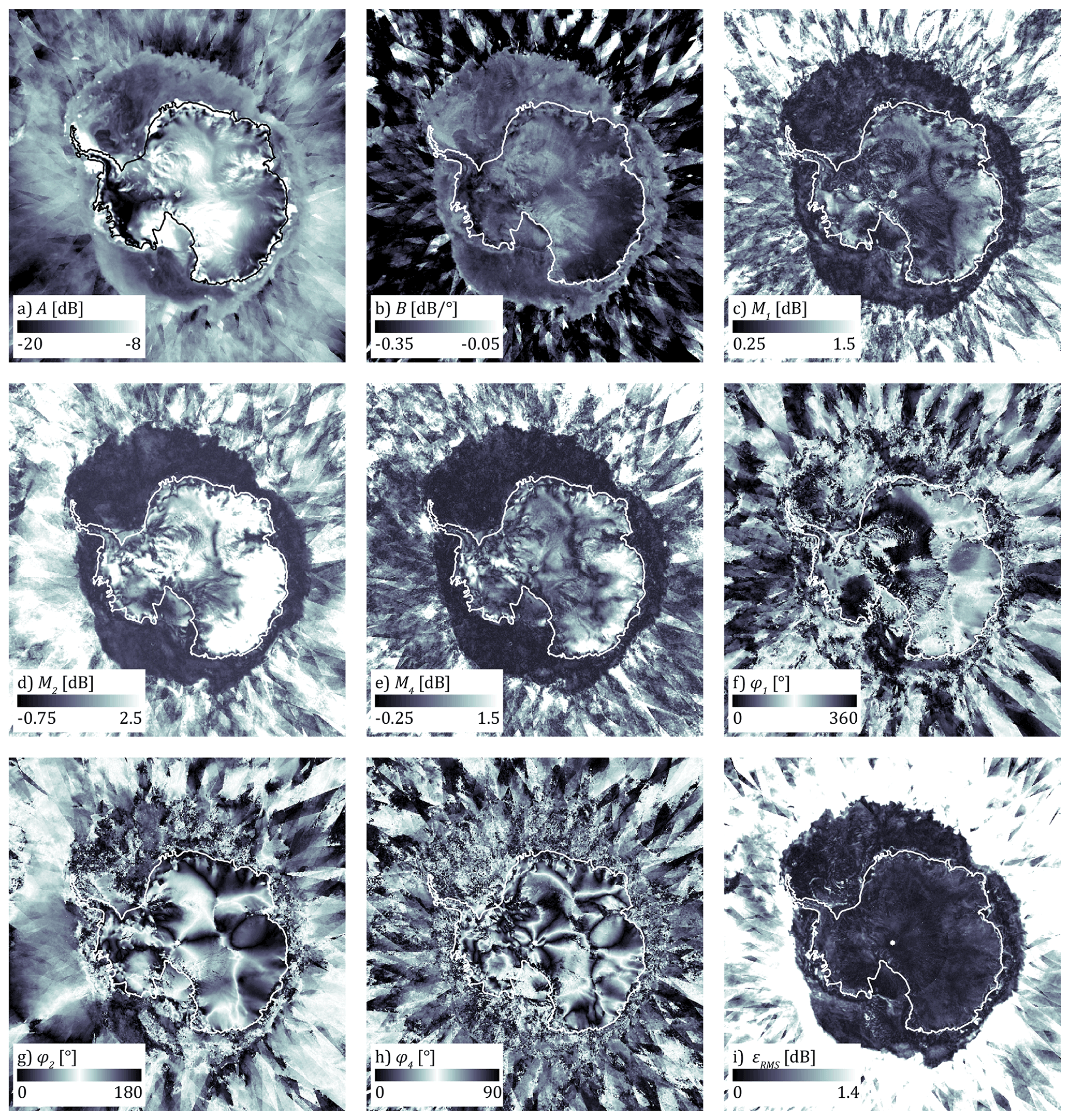
Figure 1 Example parameter maps at 2 d resolution over the Antarctica and the Southern Ocean, taken from 2017, day of year range 171–172 (20–21 April 2017) using data from MetOp-A and MetOp-B. Coastlines outlined in black (a) or white (others, b–i).

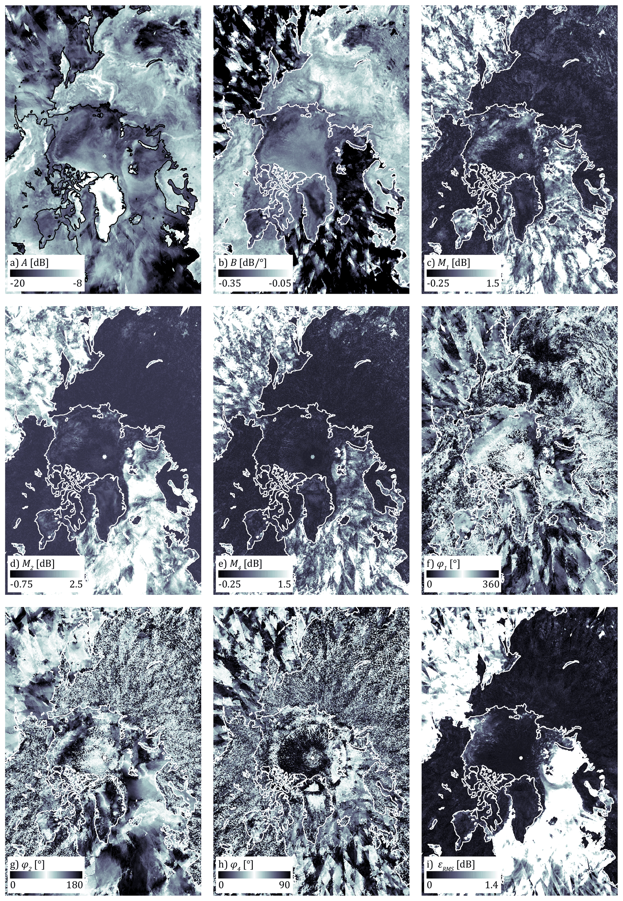
Figure 2 Example parameter maps at 2 d resolution over the Arctic, taken from 2017, day of year range 351–352 (21–22 December 2017) using data from MetOp-A and MetOp-B. Coastlines outlined in black (a) or white (b–i).

The datasets described in (b) (CERSAT and NASA SCP) represent those most closely comparable with the dataset presented here. Key differences between this dataset and those readily available stem from the more complex and computationally expensive parameterisation required to account for the azimuthal anisotropy in the backscatter measurements (seen in Fig. 3). A trade-off we make in performing a detailed anisotropy characterisation is the preclusion of parameter retrieval in regions with a limited number of observations. We retrieve a total of eight parameters, so we require at least eight observations of the surface for parameter estimation to occur. This, in turn, requires at least three ASCAT passes (each pass gives three unique observations). Products normalising only by incidence angle (e.g. CERSAT and NASA SCP) require only one pass to provide sufficient observations, yielding marginally higher coverage at latitudes further from the geographical pole (Fig. 4) and due to this an increased return rate. Figure 5 shows a direct comparison of the datasets averaged over the entirety of 2017, with both datasets gridded to the same spatial resolution. A and B parameter difference maps shown in Fig. 5c and d, respectively, indicate that the two products partition backscatter differently between these two parameters, with regions of positive A parameter difference coinciding with negative B parameter difference, and vice versa. Fig. 5f also shows the high to low azimuthal diversity zones clearly as a discontinuity in the B parameter in the SCP product, indicating that the more sophisticated parameterisation presented here handles this viewing geometry regime change more seamlessly.

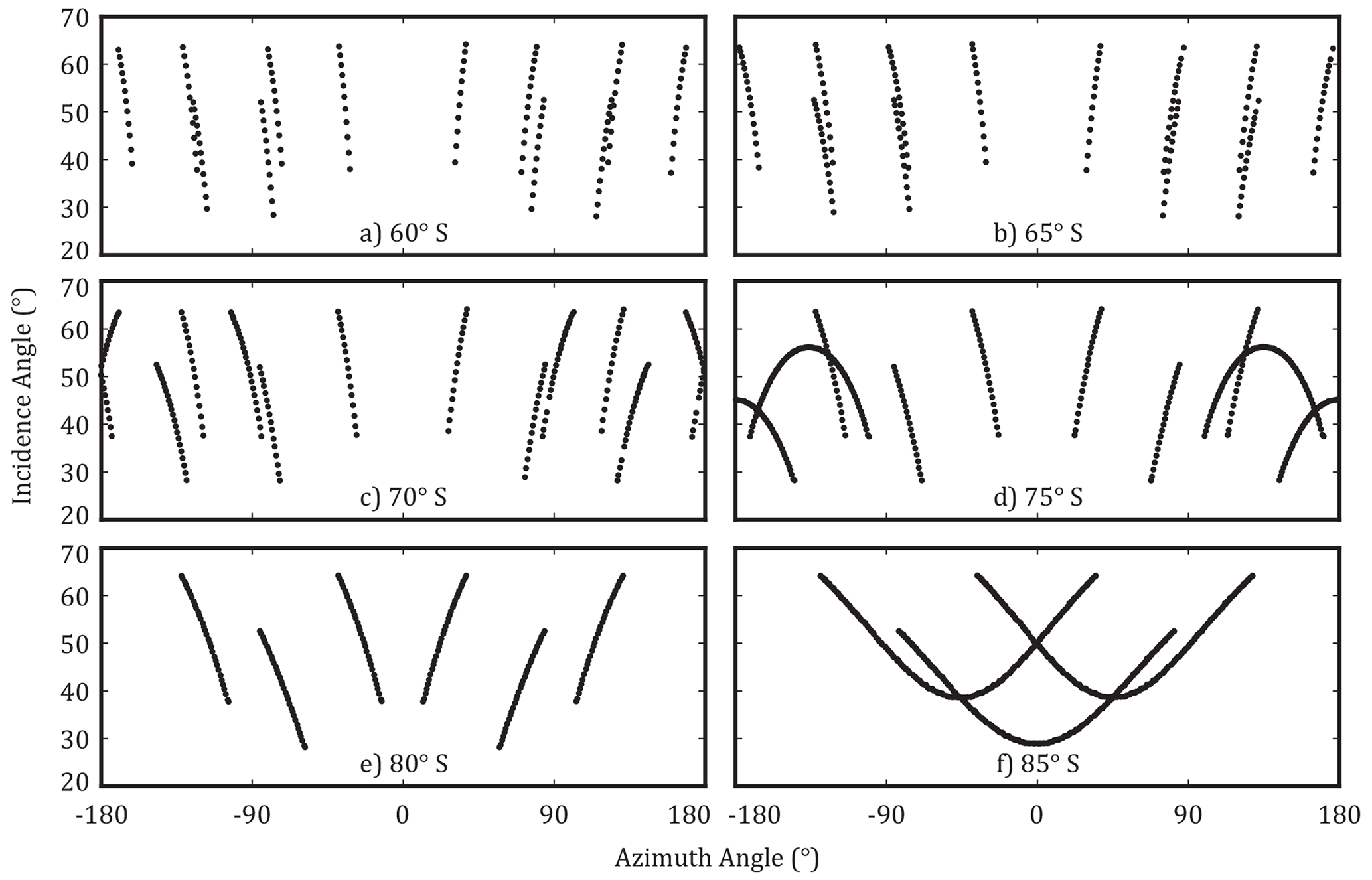
Figure 3 Plot of the azimuth and incidence angle distributions of the scatterometer swaths in the Southern Hemisphere as a function of latitude from (a) 60^∘ to (f) 85^∘ south from MetOp-B over June 2017.

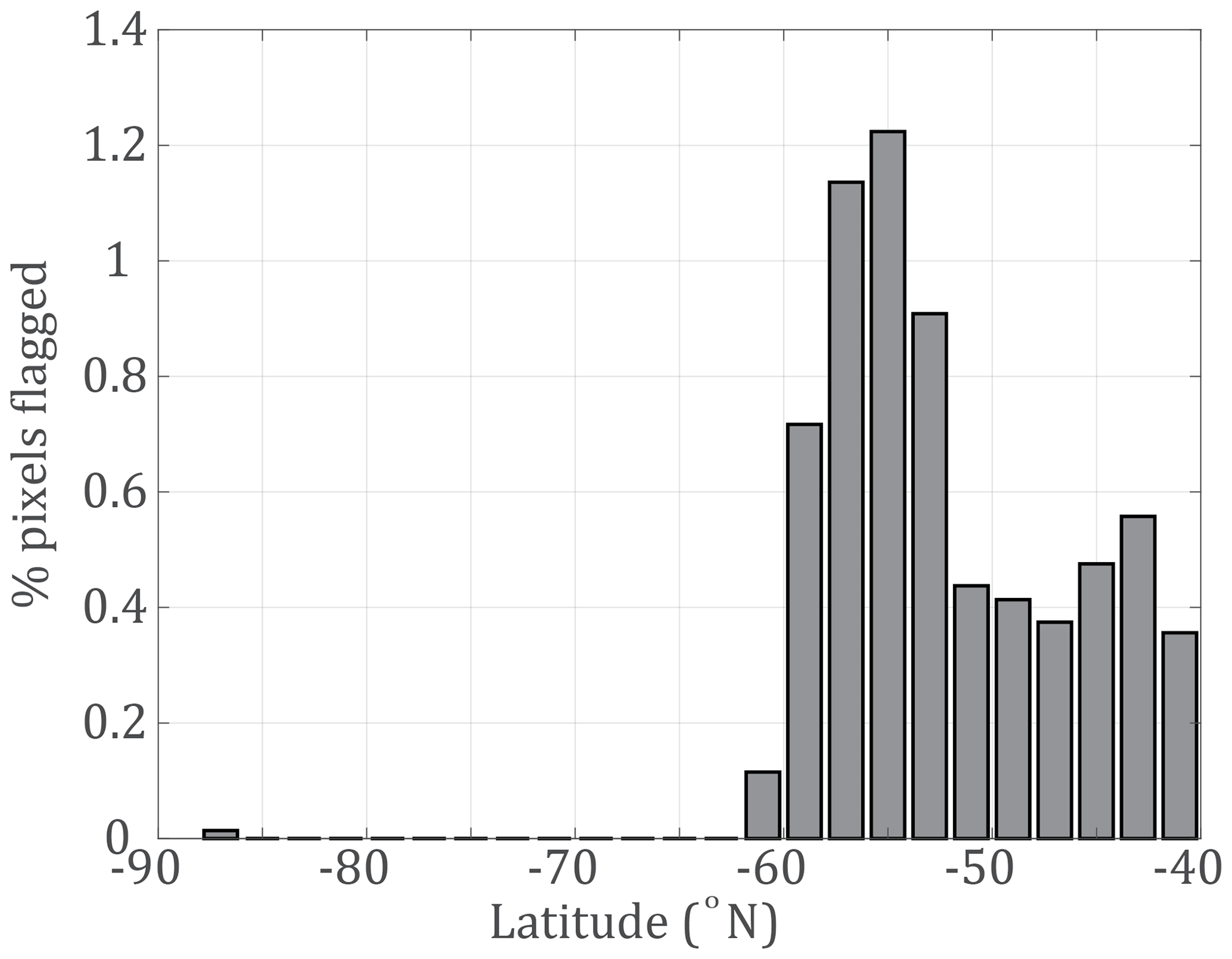
Figure 4 Invalid pixels binned by latitude as a percentage of total pixels in map for the data at 1 d resolution over the Southern Hemisphere (MetOp-A, MetOp-B and MetOp-C). These patterns will be mirrored in the Northern Hemisphere due to orbital geometry.

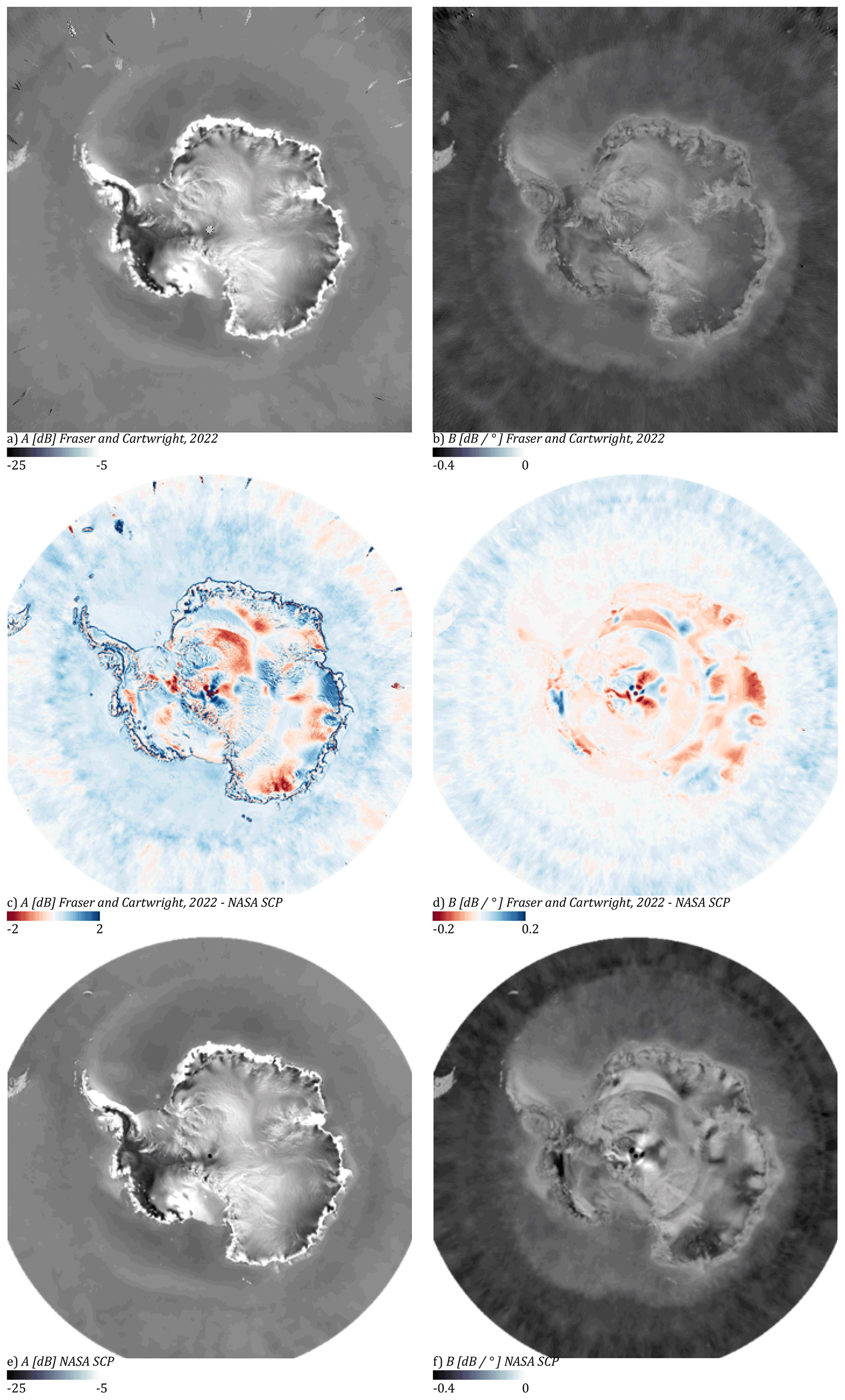
Figure 5 Comparison of NASA SCP product produced by the BYU Center for Remote Sensing and the dataset presented in this paper (without application of quality flags). Datasets are an average of 2017. Panels (a, b) correspond to the product presented here (Fraser and Cartwright, 2022), (e, f) the NASA SCP product and (c, d) the difference between the two. Panels (a, c, e) and (b, d, f) are the A and B parameters respectively.

Data from ASCAT are currently used for the characterisation of global sea ice extent, as well as ice type retrieval in the Northern Hemisphere (Breivik et al., 2012). These products are routinely produced and available from Ocean and Sea Ice Satellite Application Facility (OSI SAF – https://osi-saf.eumetsat.int/, last access: 29 January 2022). Ice extent calculations exploit the difference in backscatter received by the fore and rear antennas in combination with passive microwave sensors. A Bayesian methodology is applied with the use of training areas to identify sea ice, open water and, in the Northern Hemisphere, sea ice type (Breivik et al., 2012). Similar parameters to those used by OSI SAF for the creation of these Level 2 products may be extracted from the more comprehensive parameterisation presented here, demonstrating their use in the classification of ice surfaces and allowing these same techniques to be applied over a wider variety of applications in the cryosphere

We note that spatial-resolution-enhanced ASCAT products exist (Long et al., 1993; Vogelzang and Stoffelen, 2017) but emphasise that the present dataset focusses not on resolution but a relatively detailed parameterisation (to ensure minimal residual anisotropy) and parameter estimation with the shortest possible time interval, which is determined by the number of MetOp platforms operational at the time. In future work we hope to combine all three attributes for enhanced spatial resolution, complex parameterisation and high temporal resolution.

3 ASCAT and MetOp-A, MetOp-B and MetOp-C platforms

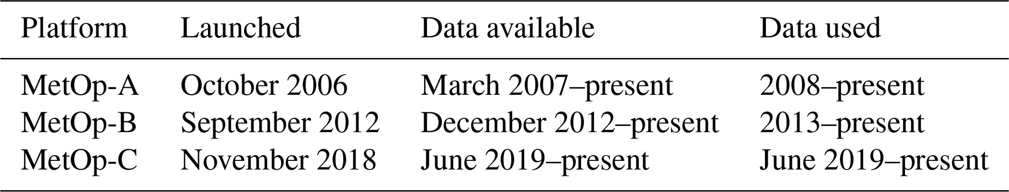
The backscatter data used in this study are acquired from the Advanced Scatterometer (ASCAT) on board MetOp-A, MetOp-B and MetOp-C. These three satellites have been put into orbit at an inclination of 98.2^∘ and an altitude of 817 km into sun-synchronous orbits with a period of 101 min (Figa-Saldaña et al., 2002). Each satellite has a 29 d repeat cycle, and a 5 d subcycle. The launch dates and data availability of each of the three satellites can be seen in Table 1 below, with the overlapping periods of data availability enabling a reduction in parameter map time step from 5 d maps before 2013 (only MetOp-A) to 2 d maps (MetOp-A and MetOp-B) and daily resolution as data become available from MetOp-C. MetOp-B and MetOp-C are in the same plane, spaced approximately half an orbit apart. Thus, with this pair alone, the orbital period is effectively reduced to 50 min. MetOp-A shares its period and inclination with MetOp-B and MetOp-C but has been drifting since 2017 to facilitate extension of its lifetime. It is now in a different plane but still providing high-quality backscatter measurements. The tri-platform observation network is projected to be operational until 2022.

Table 1 Launch dates of MetOp-A, MetOp-B and MetOp-C and data availability from each.

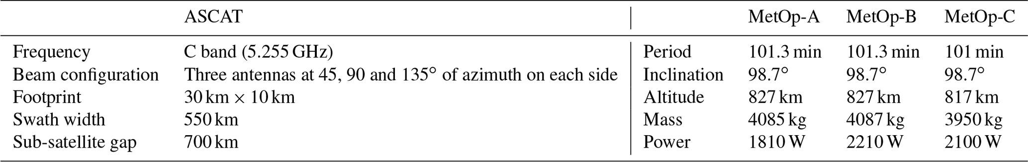
ASCAT is a C-band (5.255 GHz) VV-polarisation scatterometer with six fan-beam antennas (Table 2). The antennas give a two-swath configuration, each approximately 550 km wide, with a 720 km sub-satellite gap, measuring backscatter up to 88^∘ N/S. Three antenna pairs on each side (±45^∘, ±90^∘ and ±135^∘ of azimuth relative to the sub-satellite track) give a wide variety of azimuth and incidence angles (25–65^∘), seen in Fig. 3. Over a 5 d subcycle, these provide many looks of a region of the Earth's surface, with a high diversity of both incidence and azimuth angles (Fraser et al., 2014). The current half-orbit (50 min) spacing of MetOp-B and MetOp-C gives highly complementary coverage of polar regions; i.e. a 50 min interval corresponds to an Earth rotation of 12.5^∘. At a latitude of 65^∘ (N or S), a 12.5^∘ rotation corresponds to a distance of ∼580 km; thus at this latitude, MetOp-B and MetOp-C observe within each other's sub-satellite gap during subsequent passes. As MetOp-A's orbit is drifting, this increases the diversity of observations and allows for daily maps of the parameters given here, although the phasing of the orbit (and hence the degree to which it can be considered complementary) will drift over time.

Table 2 Instrument and platform specifications.

4 Methods

Data were acquired in NetCDF format from the European Organisation for the Exploitation of Meteorological Satellites (EUMETSAT) Data Centre (“ASCAT GDS Level 1 Sigma0 resampled at 12.5 km Swath Grid – MetOp”), data code ASCSZR1B. The 12.5 km resampled product is used here. The processing required to reach the resampled product results in a true spatial resolution of 25–30 km, as the full-resolution product is smoothed in both the across- and along-track directions for gridding. There are approximately 14 complete-orbit files per day, starting and ending near the North Pole. These files contain geographic location data for each pixel, as well as azimuth, incidence, σ₀ (normalised radar cross section or NRCS – here termed backscatter) and K_p (residual mean square of the NRCS) values in the format of triplets (fore, mid and aft antennas), each with 82 data points per row.

The ASCAT swath data are then resampled onto the NSIDC polar stereographic 12.5 km grid, EPSG 3411 and 3412 for the Northern and Southern Hemisphere respectively. This is performed separately for the Northern and Southern Hemisphere data, with true latitude at 70^∘ for each hemisphere. This grid was chosen in order to ensure wide availability of compatibility of other sea ice datasets, as well as to ensure minimal distortion of the grid in the sea ice region. This grid is 608 × 896 pixels in the Northern Hemisphere and 632 × 664 pixels in the Southern Hemisphere.

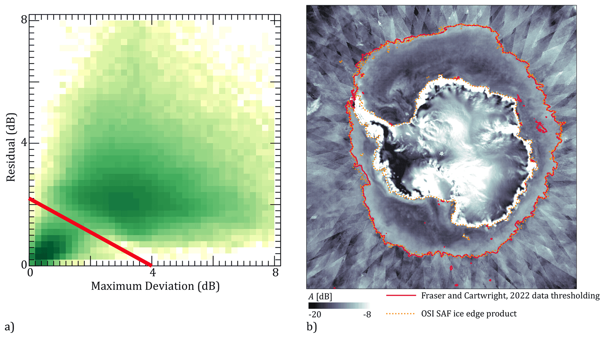
Figure 6 ​​​​​​​Application of dataset to surface type (sea ice vs open water) delineation. Date shown is DOY 271–275, 2019 (28 September–2 October 2019). (a) Simple thresholding algorithm uses low azimuthal anisotropy over sea ice in comparison to high azimuthal anisotropy of sea water to classify the two surfaces, through parameters in the dataset. (b) “A” parameter map overplotted with ice edge from this dataset (red, solid) and that of the OSISAF ice edge product (orange, dotted).

In regions exhibiting backscatter anisotropy, backscatter varies with incidence and azimuth angle, and such anisotropy needs to be characterised before physical parameter retrieval can take place. Accurate quantification of the anisotropy is undertaken by defining a model which describes the relationship between backscatter and the incidence/azimuth angles. Fraser et al. (2014) showed that a parameterisation featuring a linear falloff of incidence angle with increasing backscatter, plus a first, second and fourth harmonic sinusoidal azimuthal response, was a good choice for representing the anisotropy found on most of the Antarctic Ice Sheet. While work on sea ice parameter retrieval is still at a nascent stage, this same parameterisation shows promise in this domain too. Thus, we adopt the “Linear_124” parameterisation from Fraser et al. (2014) as a general parameterisation with a wide range of potential applications to the cryosphere. This is in contrast to other products mentioned above, modelling backscatter solely as a function of incidence angle, and presents the relationship between these as a surface as a function of the two, ${\mathit{\sigma }}_{\mathrm{0}}=A+f\left(\mathit{\theta }\right)+g\left(\mathit{\phi }\right)$, where σ₀ represents the measured backscatter, θ is the incidence angle and φ is the azimuth angle of the observation. The Linear_124 parameterisation from Fraser et al. (2014) is given in Eq. (1) below.

$$\begin{array}{}\text{(1)}& \begin{array}{rl}{\mathit{\sigma }}_{\mathrm{0}}& =A+B\left(\mathit{\theta }-\mathrm{40}{}^{\circ }\right)+m_{\mathrm{1}}\cos \left(\mathrm{1}\left(\mathit{\phi }-{\mathit{\phi }}_{\mathrm{1}}\right)\right)\\ & +m_{\mathrm{2}}\cos \left(\mathrm{2}\left(\mathit{\phi }-{\mathit{\phi }}_{\mathrm{2}}\right)\right)+m_{\mathrm{4}}\cos \left(\mathrm{4}\left(\mathit{\phi }-{\mathit{\phi }}_{\mathrm{4}}\right)\right)\end{array}\end{array}$$

Parameterisation is performed separately for the gridded data in the Northern and Southern Hemisphere and on three different timescales – every 5 d (using data from MetOp-A only), every 2 d (MetOp-A and MetOp-B) and daily parameter maps (data from MetOp-A, MetOp-B and MetOp-C). These parameters are detailed below and can be seen in Figs. 1 and 2:

• A – isotropic component of backscatter (normalised to a mid-range incidence angle of 40^∘);

• B – co-efficient describing the linear falloff of backscatter with increasing incidence angle;

• m₁ and φ₁ – amplitude and phase of fundamental azimuth anisotropy component;

• m₂ and φ₂ – amplitude and phase of bisinusoidal azimuth anisotropy component;

• m₄ and φ₄ – amplitude and phase of fourth harmonic azimuth anisotropy component;

• residual – root-mean-square difference between observations and model after parameter fitting.

These data are provided as Climate and Forecasting (CF)-compliant NetCDF4 format, with the date of each time step and all parameter maps along with the latitude and longitude grid in annual files (DOI: https://doi.org/10.26179/91c9-4783). Data flags are provided in order to identify invalid pixels where there are insufficient data within the time period to accurately parameterise (fewer than eight inputs). The coverage of the 1 d product is maximised due to the use of all three satellites; the average percentage of invalid pixels remaining separated by latitude can be seen in Fig. 4. These can be seen to increase with movement away from the poles due to the orbital geometry. For this parameterisation, as each satellite provides complete coverage every 5 d over the polar areas, the three combined require more than a day to ensure full coverage of the polar extremities. A compromise has been reached here, with the 1 d product covering the majority of the polar area and enabling a much product over many of the areas of interest. Recent drifting of MetOp-A (in order to extend its lifetime) will lead to larger gaps in the 1 d product as the orbits become more similar between the satellites.

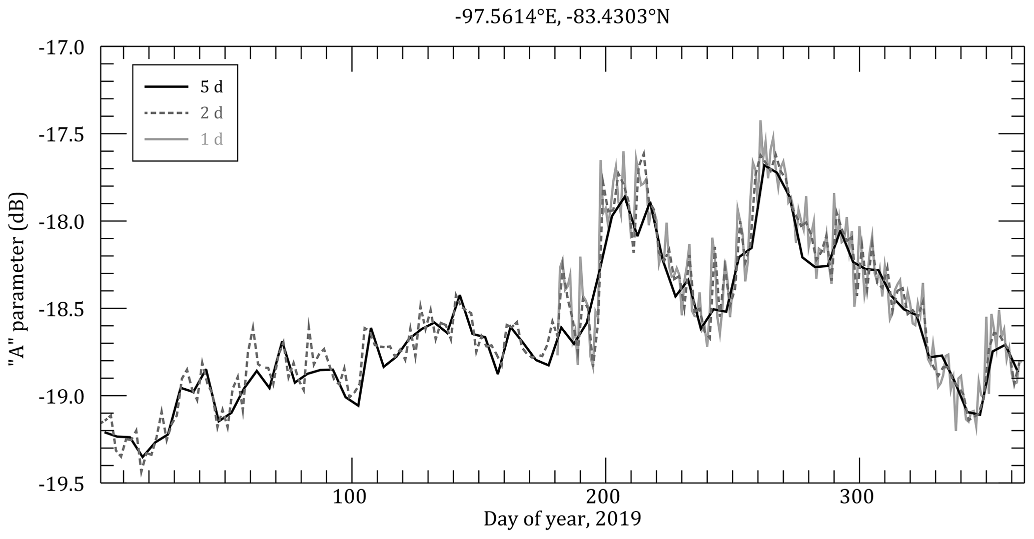
Figure 7 Comparisons of the A parameter in all three datasets, shown in decibels at a point in Antarctica for 2019. Solid black line denotes the 5 d dataset, dashed grey line the 2 d dataset and solid grey line the 1 d dataset.

5 Dataset applications

As presented in Table 1 of Fraser et al. (2014), the majority of previous studies using scatterometry in the cryosphere have applied a linear incidence angle parameterisation. Such studies would be repeatable using the B parameter provided here, in addition to those that feature the fourth-order Fourier series azimuth characterisation. It can be seen therefore that these elements are widely used in ice sheet studies, as well as sea ice extent and type as seen in the OSI SAF product (Breivik et al., 2012). Figure 6 shows an application of this dataset in the form of an accurate ice edge product, comparable with that of OSI SAF (OSI SAF, 2019b). The algorithm presented here emulates that of OSI SAF by assuming the sea ice azimuthal anisotropy is low in comparison to that of open water. Figure 6a shows a two-dimensional histogram of parameter fit residual (y axis) vs “maximum deviation” (x axis). The maximum deviation metric is calculated as the maximum absolute deviation, in decibels (dB), of σ₀ as a function of azimuth, when using the six Fourier parameters presented in this dataset. Sea ice pixels have a low residual and low maximum deviation, while ocean pixels have a high residual and maximum deviation. Partitioning using one parameter alone cannot separate these classes; however combining these two parameters allows for effective separation of the two surface types (here separated by the red line in Fig. 6a). Figure 6b shows the resulting ice edge (red line), as well as the OSI SAF ice edge (dotted orange line). Polynyas off Cape Darnley and the Ross Ice Shelf are visible along with a gap in the ice off Prydz Bay, that is also visible in concentration data from the day (not shown). Further elucidation of this application is outside of the scope of this paper.

The data presented here are suitable for a wide array of cryosphere studies, including sea and glacial ice, as is visible in Figs. 1 and 2, with changes seen across the sea ice pack and in the varying geographic and climatological zones of the polar regions. These uses are shown by previous applications of the ASCAT Sigma0 data. Here these data are taken a step further than the incidence angle parameterisations, additionally accounting for azimuth angle. These data are provided on standard grids (NSIDC polar stereographic) in both hemispheres and across a variety of temporal resolutions in order to ensure full geographic coverage, using the sensors on board all three MetOp satellites and taking advantage of the impressive coverage and consistency of the ASCAT dataset. We provide an extended time series of parameters covering 13 years in the case of the coarsest temporal resolution. The comparison of the three time steps seen in Fig. 7 reveals that the longer averaging period of the 5 d product limits the sensitivity to shorter scale changes. The 5 d dataset therefore creates a less noisy dataset for point comparisons and allows for full use of the decadal timescale of the ASCAT instruments.

In the future we hope to be able to build and extend this dataset with the launch of the EUMETSAT polar system second-generation (EPS-SG) MetOp-SG series, three satellites with proposed SCA scatterometers on board due to launch in 2024 (Lin et al., 2012). These aim to provide comparable measurements to ASCAT but with a finer horizontal resolution and a wider swath (Lin et al., 2012).

6 Data availability

The​​​​​​​ source data used for the derivation of these parameters are available from the EUMETSAT Data Centre (https://vnavigator.eumetsat.int/product/EO:EUM:DAT:METOP:ASCSZR1B, EUMETSAT, 2021), under the product “ASCAT GDS Level 1 Sigma0 resampled at 12.5 km Swath Grid – MetOp”, data code ASCSZR1B. The data presented in this paper are available from the Australian Antarctic Data Centre, https://doi.org/10.26179/91c9-4783 (Fraser and Cartwright, 2022).

7 Conclusion

Here we present a new dataset of scatterometry parameterisations taking advantage of the complete constellation of MetOp satellites in orbit. The use of three platforms (MetOp-A, MetOp-B and MetOp-C) allows multiple temporal resolutions of the product to be provided and full parameterisations to be achieved, accounting for both incidence and azimuth angle anisotropy. In this, the product is unique. It is hoped that this parameterisation, proven for cryosphere purposes (Fraser et al., 2014), will encourage the exploitation of scatterometry data for cryosphere science, research and monitoring. This dataset will be updated through the lifetime of the MetOp platforms and will aim to be continued with the launch of the first of the MetOp-SG series in 2024.