the Creative Commons Attribution 4.0 License.
the Creative Commons Attribution 4.0 License.
 | 20 Oct 2022
The Green Edge cruise: investigating the marginal ice zone processes during late spring and early summer to understand the fate of the Arctic phytoplankton bloom
Flavienne Bruyant
Rémi Amiraux
Marie-Pier Amyot
Philippe Archambault
Lise Artigue
Lucas Barbedo de Freitas
Guislain Bécu
Simon Bélanger
Pascaline Bourgain
Annick Bricaud
Etienne Brouard
Camille Brunet
Tonya Burgers
Danielle Caleb
Katrine Chalut
Hervé Claustre
Véronique Cornet-Barthaux
Pierre Coupel
Marine Cusa
Fanny Cusset
Laeticia Dadaglio
Marty Davelaar
Gabrièle Deslongchamps
Céline Dimier
Julie Dinasquet
Dany Dumont
Brent Else
Igor Eulaers
Joannie Ferland
Gabrielle Filteau
Marie-Hélène Forget
Jérome Fort
Louis Fortier
Martí Galí
Morgane Gallinari
Svend-Erik Garbus
Nicole Garcia
Catherine Gérikas Ribeiro
Colline Gombault
Priscilla Gourvil
Clémence Goyens
Cindy Grant
Pierre-Luc Grondin
Pascal Guillot
Sandrine Hillion
Rachel Hussherr
Fabien Joux
Hannah Joy-Warren
Gabriel Joyal
David Kieber
Augustin Lafond
José Lagunas
Patrick Lajeunesse
Catherine Lalande
Jade Larivière
Florence Le Gall
Karine Leblanc
Mathieu Leblanc
Justine Legras
Keith Lévesque
Kate-M. Lewis
Edouard Leymarie
Aude Leynaert
Thomas Linkowski
Martine Lizotte
Adriana Lopes dos Santos
Claudie Marec
Dominique Marie
Guillaume Massé
Philippe Massicotte
Atsushi Matsuoka
Lisa A. Miller
Sharif Mirshak
Nathalie Morata
Brivaela Moriceau
Philippe-Israël Morin
Simon Morisset
Anders Mosbech
Alfonso Mucci
Gabrielle Nadaï
Christian Nozais
Ingrid Obernosterer
Thimoté Paire
Christos Panagiotopoulos
Marie Parenteau
Noémie Pelletier
Marc Picheral
Bernard Quéguiner
Patrick Raimbault
Joséphine Ras
Eric Rehm
Llúcia Ribot Lacosta
Jean-François Rontani
Blanche Saint-Béat
Julie Sansoulet
Noé Sardet
Catherine Schmechtig
Antoine Sciandra
Richard Sempéré
Caroline Sévigny
Jordan Toullec
Margot Tragin
Jean-Éric Tremblay
Annie-Pier Trottier
Daniel Vaulot
Anda Vladoiu
Lei Xue
Gustavo Yunda-Guarin
Marcel Babin
The Green Edge project was designed to investigate the onset, life, and fate of a phytoplankton spring bloom (PSB) in the Arctic Ocean. The lengthening of the ice-free period and the warming of seawater, amongst other factors, have induced major changes in Arctic Ocean biology over the last decades. Because the PSB is at the base of the Arctic Ocean food chain, it is crucial to understand how changes in the Arctic environment will affect it. Green Edge was a large multidisciplinary, collaborative project bringing researchers and technicians from 28 different institutions in seven countries together, aiming at understanding these changes and their impacts on the future. The fieldwork for the Green Edge project took place over two years (2015 and 2016) and was carried out from both an ice camp and a research vessel in Baffin Bay, in the Canadian Arctic. This paper describes the sampling strategy and the dataset obtained from the research cruise, which took place aboard the Canadian Coast Guard ship (CCGS) Amundsen in late spring and early summer 2016. The sampling strategy was designed around the repetitive, perpendicular crossing of the marginal ice zone (MIZ), using not only ship-based station discrete sampling but also high-resolution measurements from autonomous platforms (Gliders, BGC-Argo floats …) and under-way monitoring systems. The dataset is available at https://doi.org/10.17882/86417 (Bruyant et al., 2022).
- Article
(10913 KB) - Full-text XML
- BibTeX
- EndNote


The Arctic Ocean is currently experiencing unprecedented environmental changes. The increase of the summer ice retreat lengthens the phytoplankton growing season but also increases the area of the marginal ice zone (MIZ). If trends are maintained, all Arctic sea ice may become seasonal as early as 20 years from now (Meredith et al., 2019), increasing the MIZ coverage even more. Ice edge blooms represent much of the annual phytoplankton primary production in the Arctic Ocean (Perrette et al., 2011; Ardyna et al., 2013), and their current phenology is relatively well known (Wassmann and Reigstad, 2011; Leu et al., 2015). However, we currently do not know how precisely primary production will respond to climate changes. The overarching goal of Green Edge was to understand the processes that control an Arctic phytoplankton spring bloom (PSB) as it expands northward and to determine its fate through the investigation of related carbon fluxes (e.g., Trudnowska et al., 2021). This study was also motivated by the discovery that PSBs can and do occur underneath the ice (Arrigo et al., 2014) despite the limited amounts of under-ice available light (Mundy et al., 2009; Arrigo et al., 2014; Lowry et al., 2014; Assmy et al., 2017; Randelhoff et al., 2019). Field studies for the Green Edge project were carried out in 2015 and 2016 at an ice camp located on landfast sea ice close to Qikiqtarjuaq (NU, Canada). Additionally, during late spring and early summer 2016, a cruise aboard CCGS Amundsen was conducted in Baffin Bay. As explained in Randelhoff et al. (2019), Baffin Bay is both relatively easy to access and represents an ideal framework for this study, because environmental conditions are representative of what is observed at the pan-Arctic scale. Particularly, the warm Greenland current, flowing north on the Greenland side, and the colder waters on the Canadian side, flowing south (Baffin Island current), induce an evenly retreating ice edge, allowing a straightforward sampling strategy. From the Green Edge project, two separate data papers were produced. One paper by Massicotte et al. (2020) describes the dataset generated during two ice-camp campaigns on landfast ice (2015 and 2016). The latter paper is related to a dataset published in 2019 on SEANOE: https://www.seanoe.org/data/00487/59892/ (last access: 28 September 2022). The second paper (the present paper by Bruyant et al., 2022) provides an overview of the dataset gathered during an oceanographic cruise conducted in Central Baffin Bay in 2016. For more clarity, we created a second dataset on SEANOE associated with the present paper: https://doi.org/10.17882/86417 (Bruyant et al., 2022). This 2022 DOI contains the final version of all the cruise data that could be formatted to be published by SEANOE (see Sect. 6 Data availability). Note that the first dataset (Massicotte et al., 2020) contained some of the cruise data for the sake of contextualizing the ice-camp dataset.
Table 1List of operations carried out during the Green Edge cruise at each different station type. [(+) Opportunistic sampling only]. CTD conductivity–temperature–depth; AOP apparent optical properties; C-OPS Compact-Optical Profiling System; IOP inherent optical properties; BB9 backscattering meter; CDOM coloured dissolved organic matter; SCAMP Self-Contained Autonomous MicroProfiler; LOKI Lightframe On-sight Key species Investigation.
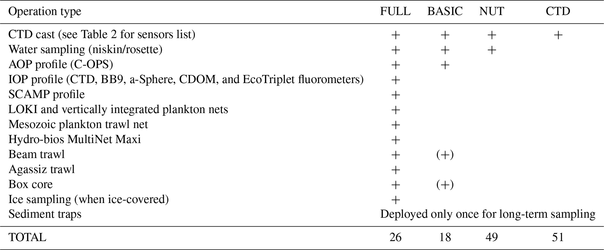

Figure 1Cruise maps showing (a) the seven transects and all stations with shape distinction between station type (FULL, BASIC, NUT, and CTD, see Table 1 for description). Coloured lines indicate the position of the ice edge (sea-ice concentration at 80 %) on each transect at the date of sampling; ice cover persisted on the western side of Baffin Bay, while the eastern side cleared earlier. The starting date of each transect sampling is as follows: 9 June (100), 14 June (200), 17 June (300), 24 June (400), 29 June (500), 3 July (600), and 7 July (700). (b) Tracks of the four BGC-Argo floats deployed during the Green Edge cruise over their first 101 d of life, and the journey of the two SLOCUM gliders (blue and orange). The dashed line represents the ship track along the seven transects.
For logistical reasons, the cruise was divided into two legs. Leg 1A started on 3 June in Québec City, ended on 23 June in Qikiqtarjuaq (NU), and included one week of transit to the study zone. Leg 1B started on 23 June in Qikiqtarjuaq and ended in Iqaluit (NU) on 14 July. During the five-week period spent in Baffin Bay, the ship crossed the MIZ, from open waters (in the east) to sea-ice-covered areas (in the west) and back again following latitudinal transects. A total of seven transects were covered between 68.0 and 70.5∘ N (Fig. 1a). Three transects were covered during Leg 1A (68.5 to 69.0∘ N) and four during Leg 1B (68.0 and 69.5 to 70.5∘ N). For each transect, stations were separated by six nautical miles (approximately 11 km) to obtain a relatively high spatial resolution. A total of 15 to 25 stations were sampled within each transect, for a total of 144 stations visited during the campaign.
Table 2List of the sensors attached to the rosette carousel. CDOM coloured dissolved organic matter; PAR photosynthetically available radiation; ADCP acoustic Doppler current profiler; UVP Underwater Vision Profiler. NA – not available.
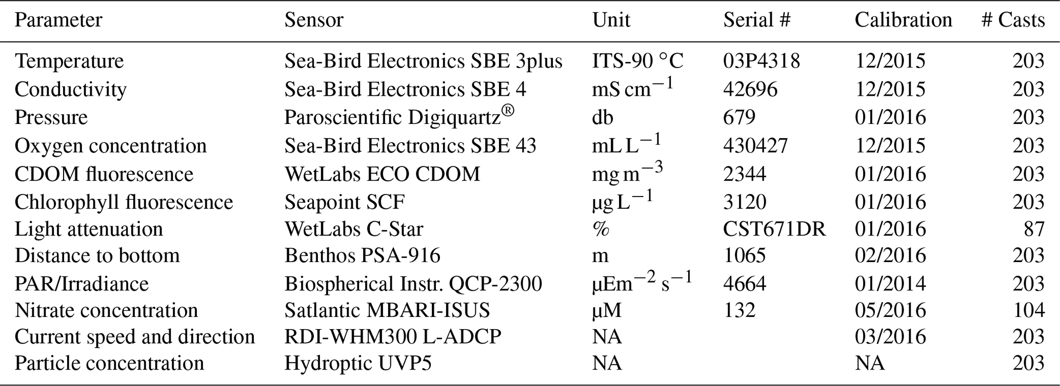
The activities conducted at each type of station are detailed in Table 1. Briefly, at so-called CTD (current temperature depth) stations, rosette casts did not include seawater collection. The rosette, a Sea-Bird model 32 carousel equipped with 22 12 L Niskin bottles, was geared with multiple sensors (see Table 2 for details). At NUT stations, seawater samples were additionally collected at several depths between 2 and 2000 m for nutrient analyses. At BASIC stations, the apparent optical properties of seawater were measured using underwater profiling optical instruments. The variables measured at BASIC stations included the concentration of chlorophyll a, phytoplankton pigment, particulate carbon and nitrogen, and particulate absorption spectra. Finally, at FULL stations, a suite of measurements was made on seawater samples, and several underwater instruments were deployed as well, including a suite of optical sensors. Vertical plankton nets geared with a plankton imager, horizontal net trawls, benthic trawls, and Ursnel box corers were also deployed at each FULL station. Note that the number of variables measured on seawater samples was significantly larger at FULL stations, where three rosette casts were necessary to cover the demand in water volume, compared with one rosette at BASIC stations. At least one FULL station was sampled in each of the three major domains covered by each transect, namely open waters, the MIZ, and the ice-covered area. During Leg 1B, a larger emphasis was placed on collecting ice cores for analyses and measurements of light propagation through the ice and snow. FULL stations sampled in the ice-covered domain did not include trawling operations.
Our sampling strategy allowed successive crossings of different PSB stages: the early-bloom stage at the western end of transects covered in sea ice, late- to post-bloom stages at the eastern end of transects in open waters, and full-bloom stage in the middle of transects around the ice edge (see Randelhoff et al., 2019). Between the stations, the ship track water monitoring system (TSG SBE45 from Sea-Bird, WETStar fluorometer from WetLabs, LiCOR non-dispersive infra-red spectrometer (model Li-7000), Campbell Scientific CR1000 data logger) recorded temperature, salinity, chlorophyll a fluorescence, and pCO2 at 7 m depth continuously when navigating outside the ice pack. A moving vessel profiler (MVP300-1700, AML Oceanographic, Victoria BC, Canada), equipped with a micro CTD (AML), a WetLabs C-Star transmissometer, and a WetLabs Eco-FLRTD fluorometer, was deployed in open waters.
To significantly extend the monitoring of the PSB beyond the duration and space covered by the cruise, we deployed four BGC-Argo (Bio-Geo-Chemical-Argo) floats on 9 July. They collected data until late fall (Fig. 1b), performing a 0–1000 m profile each day. The ice-specific version of BGC-Argo floats that was deployed, the so-called PRO-ICE, is commercialized by NKE Electronics (France). These floats carry a typical biogeochemical payload (Sea-Bird 41 ARGO CTD, Aanderaa optode 4330 Oxygen sensor, Sea-Bird™ OCR-504 PAR (photosynthetic available radiation) and downwelling radiance sensor (380, 412 and 490 nm), Sea-Bird ECO-FLBBCD fluorescence chlorophyll-a, coloured dissolved organic matter (CDOM), and backscattering sensor and Sea-Bird SUNA nitrate sensor). They also include a 2 way-directional Iridium communication Rudics for data transmission and a sea-ice detection system to protect the float from hitting sea ice on ascent (Le Traon et al., 2020; André et al., 2020). The 2016 data are available on the following website: http://www.obs-vlfr.fr/proof/ftpfree/greenedge/db/DATA/FLOATS/ (last access: 3 October 2022).

Figure 2Comparison between salinity (psu, a), temperature (∘C, a), chlorophyll fluorescence (relative units, b), and backscattering at 700 nm (bbp(700), m−1, c); data from the qala2 glider and the takapm005b BioArgo float at their closest common position (Fig. 1b).
Figure 3Chlorophyll fluorescence measured by the Glider qala2 during its 23 d journey (Fig. 1b).
Two SLOCUM G2 gliders (Teledyne Marine Inc.) were deployed during the cruise from the ship's zodiac, either to revisit transects or in areas that were not visited by the CCGS Amundsen (Fig. 1b). They both carried a similar scientific payload and communication system as the BGC-Argo floats, rendering the possibility of inter-calibration (Fig. 2). Gliders were primarily used in the MIZ, where a 90 m icebreaker would disturb the fragile hydrological structure of shallow under-ice water masses. Gliders were deliberately directed through the same area as the BGC-Argo floats to compare CTD and optical data from both platforms. Results in Fig. 2 show a good agreement for the data. Gliders travel following a programmed sawtooth pattern, joining pre-defined waypoints. Data and instructions were transmitted both ways via iridium when the glider surfaced. Figure 3 shows an example of the level of detail provided by the gliders when travelling through complex water structures. Representing chlorophyll fluorescence measured over a three-week journey covering almost 500 km, the data show that the glider(s) did travel through both surface blooms and a subsurface chlorophyll maximum between 20–50 m. The data presented in Fig. 3 represents 693 000 chlorophyll fluorescence measurements. These constitute robust results towards the validation of the use of multiple measurement platforms to investigate complex systems.
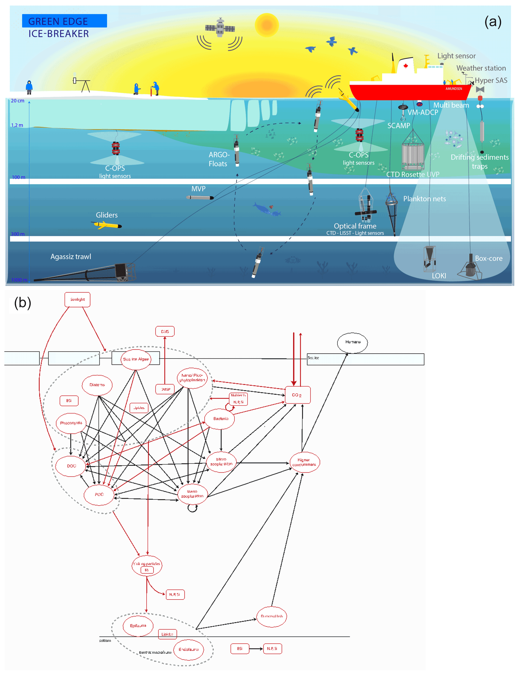
Figure 4(a) Representation of all operations carried out during the Green Edge campaign. (b) Schematic representation of all stocks (bubbles) and fluxes (arrows) measured during the Green Edge cruise as part of the MIZ trophic system. Measured and calculated variables are represented in red.
A schematic synopsis of all operations carried out during the campaign can be found in Fig. 4a. The use of multiple analysis platforms allowed the measurement of more than 150 parameters during the Green Edge cruise (Table 3); together, they accurately describe the complexity of the MIZ trophic systems (Fig. 4b) and most of the stocks and processes involved in the development of the PSB.

One of the challenging tasks when assembling data from a large group of researchers is to adopt a common frame for spatial and temporal tagging of samples. Geographic positions require a lot of attention and conversion of latitude and longitude into one format (we used decimal degrees east) to ensure data that can be easily merged. The concomitant use of local time and Coordinated Universal Time (UTC) during the cruise also presented a challenge. For the Green Edge cruise, an operation logbook was created to keep track of all operations conducted on the ship in sequential order during each day (local time). Each operation was associated with a unique operation ID to which all other data could be referenced. The use of ordinal date (number of days since January first) was used to avoid confusion between European and American date writing conventions. Each cast within a given operation type (CTD/RO for Rosette, AOP for apparent optical properties, etc.) was numbered sequentially, starting from 001, throughout the entire cruise. As a result, any given operation received a unique code, which could be used thereafter to merge all the data acquired during that operation.
Table 4Name and description of variables systematically included in datasets (i.e., in each .csv file).
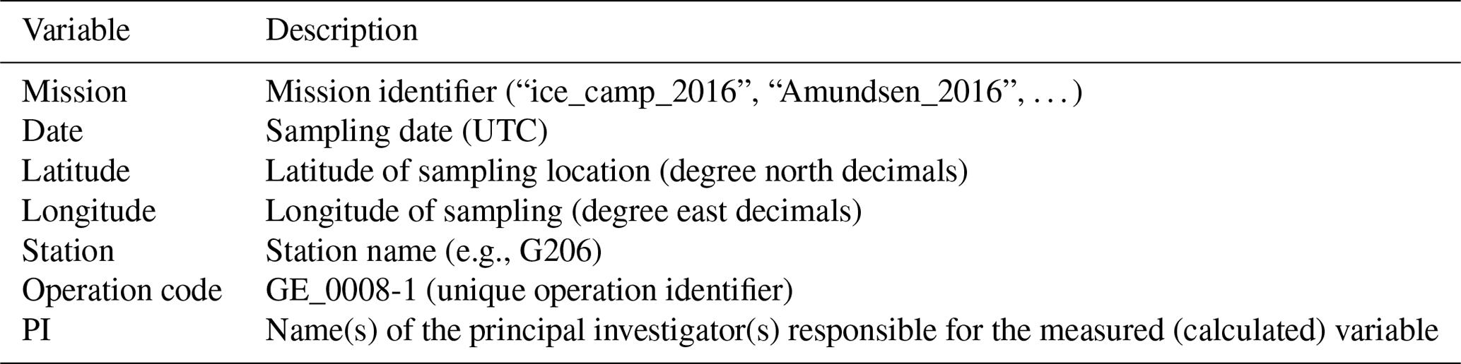
Different control procedures were adopted to ensure the quality of the data. First, the raw data were screened to identify and, where possible, eliminate errors originating from the measurement devices, including sensor (systematic or random) errors inherent to measurement procedures and methods. Instrumental pre- and post-calibration corrections were applied when necessary. Statistical summaries such as average, standard deviation, and range were computed to detect and remove anomalous values in the data. Then, data were checked for duplicates and remaining outliers. Once raw measurements were cleaned, data were structured and gathered into single, comma-separated value (CSV) files. Each of these files was constructed to gather variables of the same nature (e.g., nutrients). In each file, a minimum number of variables (columns) was always included to make dataset merging easier and accurate (Table 4).
4.1 Meteorological, navigational, and ice coverage data
Along the ship track, an automated Voluntary Observing Ship (AVOS) system recorded all data related to navigation, including the position of the vessel and basic atmospheric meteorological data (including barometric pressure). A meteorological tower was also installed on the foredeck of the ship to measure additional variables (instantaneous wind speed and direction, air temperature and relative humidity, atmospheric partial pressure, and vertical fluxes of CO2. Averaged wind speeds and directions over the entire Baffin Bay were retrieved from the Remote Sensing Systems website (http://www.remss.com/measurements/ccmp/, last access: 25 April 2021) and were computed according to the cross-calibrated multi-platform (CCMP) wind vector analysis product (V2.0, Atlas et al., 2011) (see one example of a pattern calculated over the months of June and July in Fig. 5). A major change in wind patterns happened between June (light 1–2 m s−1 southward winds) and July (4–5 m s−1 northward winds), which impacted sea ice movements. Figure 6 shows sea-ice cover over four periods covering the total sampling time of the cruise (https://nsidc.org/data/g02186, last access: 26 February 2021; NSIDC (U.S. National Ice Center and National Snow and Ice Data Center, 2010)). The north–south general orientation of the ice edge is visible, along with, over time, the westward progression of the MIZ.

Figure 5Average wind direction and speed (arrow length and colour) over Baffin Bay in June 2016 (a) and July 2016 (b); CCMP wind vector analysis product (V2.0, Atlas et al., 2011).
Ice cover history was compiled and expressed as open water days (OWD) before sampling day (Fig. 7), calculated from the difference (in day number) between the date of sampling and the date at which the sea-ice concentration reached 10 (panel A), 50 (panel B), and 80 % (panel C) in the geographical location under study. Ice concentration data were obtained from the Advanced Microwave Scanning Radiometer 2 (AMSR2) sea-ice concentration data on the 3.125 km grid (Spreen et al., 2008), downloaded from http://www.iup.uni-bremen.de:8084/amsr2data/asi_daygrid_ swath/n3125/ (last access: 18 September 2020) (see Randelhoff et al., 2019 for details on the calculations). In Fig. 7, yellow and pale green colours on the Greenland side indicate a positive value between 20 and 40 OWD, which reflects how long the open-water conditions had prevailed at those stations at the time of sampling. To the east, closer to the Canadian side, the colder colours and negative values indicate the presence of sea ice. Open water days is a useful metric or index and can be computed using different sea-ice cover (SIC) thresholds, depending on the goal. For example, in Randelhoff et al. (2019), the SIC value used for hydrological interpretation was 10 % (as in Fig. 7, top panel). However, a biologist might want to consider a SIC of 80 % (Fig. 7, bottom panel) when looking for the onset of phytoplankton growth, as only 20 % of open water surface already dramatically increases the amount of light available.

Figure 6Average weekly sea-ice extent for each of the four 8 d periods during the Green Edge cruise. Date is the median date of each 8 d sampling period. The white areas represent sea ice and the blue areas the open water. Black lines represent the ship route during said 8 d period.
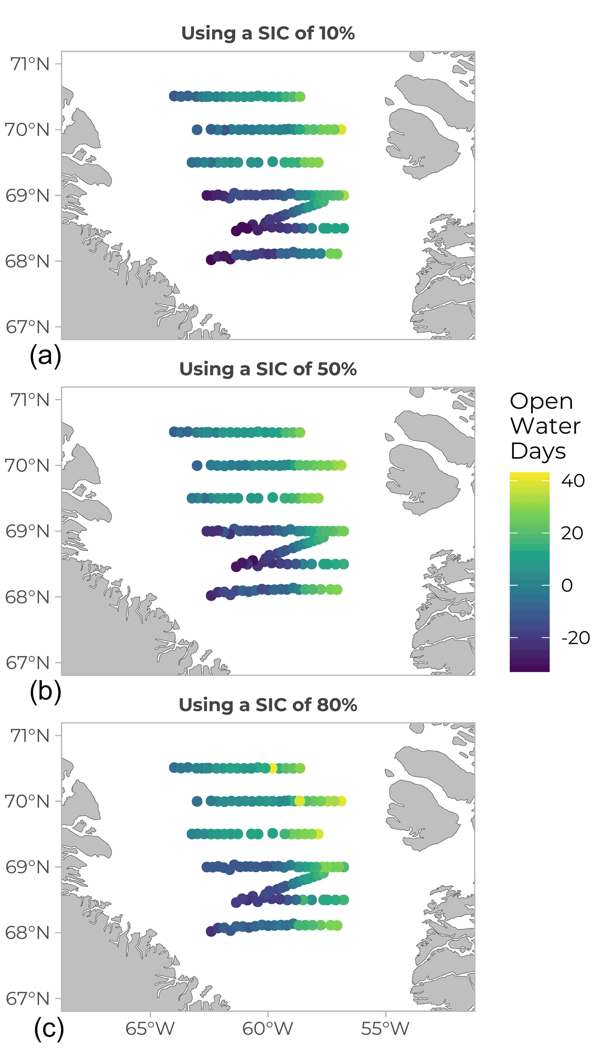
Figure 7Open water days (OWD) before sampling (values in days). The yellow colour corresponds to positive values, meaning the water was already free of ice on the day of sampling. Bluer, darker values correspond to stations that were still covered in ice at the sampling date (negative values). Values of OWD can be computed using different SIC (sea-ice coverage) values: (a) SIC =10 %, (b) SIC =50 % and (c) SIC =80 %.
4.2 Physical data
4.2.1 Sea ice
During sea-ice sampling operations, snow depth, ice thickness, and freeboard were measured at each ice-coring site. Over the cruise, ice thickness varied between 32 and 108 cm, while freeboard varied between 10 and −8 cm (top of the ice under water). Several cores were retrieved at each site using a 9 cm diameter Mark II ice corer (Kovacs Enterprises Inc., Roseburg, OR, USA). Each ice core was sliced into 10 cm segments (from the bottom) after temperature was measured. Salinity was assessed after thawing and filtration using a salinometer (Guildline Autosal 8400B, Guildline Instruments Ltd., Smith Falls, ON, Canada). Snow density and granulometry were assessed opportunistically (Eicken et al., 2009).
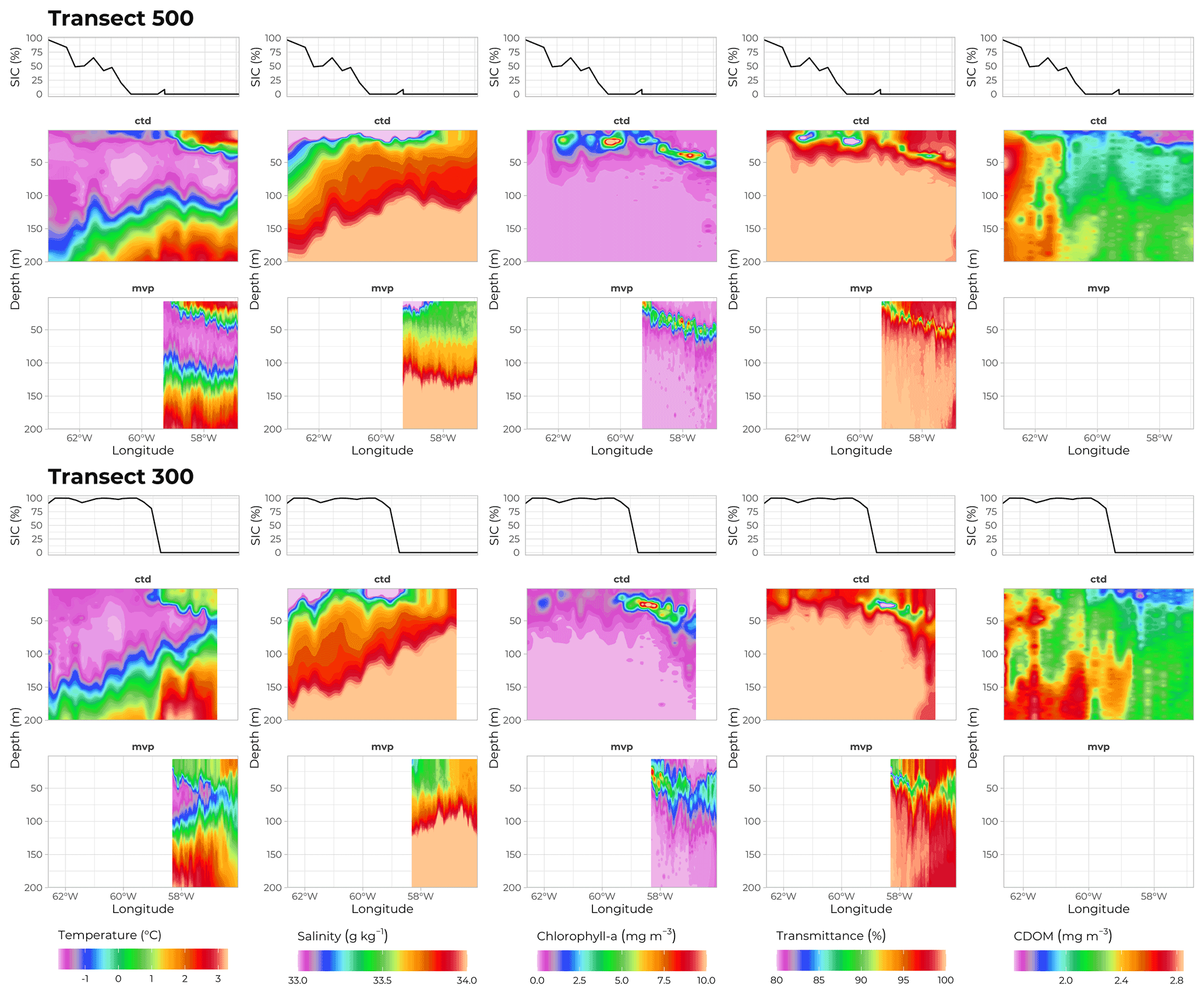
Figure 8Physical properties of seawater along transects 500 (70∘ N) and 300 (69∘ N). Middle and bottom panels show data recorded by sensors deployed on the rosette and on the MVP, respectively. From left to right: temperature (∘C), salinity (g kg−1), chlorophyll a concentration (mg m−3), transmittance (%), and CDOM concentration (mg m−3) as a function of depth (m, y axis) and longitude (∘W, x axis). Topmost panels show ice coverage (%) at corresponding longitudes. Note that the MVP did not carry a CDOM sensor.
4.2.2 Water masses
Hydrological conditions during the cruise were determined using several tools. A Moving Vessel Profiler (MVP) was deployed, oscillating between 0 and 300 m depth while towed at an average speed of 12 knots, rendering a very high spatial resolution (Fig. 8, bottom row, one profile every 2 km). Data obtained with the MVP matched the patterns observed from the rosette data acquired on sampling stations (Fig. 8, middle row). Profiles of conductivity, temperature, and pressure were collected using a Sea-Bird SBE 911plus CTD system rigged on the rosette. The data were post-processed according to the standard procedures recommended by the manufacturer and averaged over 0.2 m vertical bins. While there was a sharp transition in SIC at the ice edge along transect 300, the change in SIC was less steep in the more extensive MIZ of transect 500 (top row in Fig. 8). Nonetheless, both transects show similar patterns, with 100 % SIC and colder (below −1 ∘C) and fresher (salinity below 33.5 g kg−1) waters close to the surface on the western side, and 0 % SIC and saltier (above 33.6 g kg−1) and warmer (above 0 ∘C) waters within the first 50 m on the eastern side. These observations were consistent with the northward inflow of Atlantic-origin waters along the Greenland shelf break and the southward outflow of Arctic/Pacific-origin waters along the Baffin Island shelf break.
Currents in the water column were measured using a hull-mounted 150 kHz acoustic Doppler current profiler (ADCP, Teledyne RD Instruments Ocean Surveyor, California, USA) as well as two L-ADCP installed on the rosette structure (RDI, WHM300-1-UG304) in a master/slave configuration. Vertical profiles of water turbulence were measured at each FULL station using a Self-Contained Autonomous MicroProfiler (SCAMP, Precision Measurement Engineering, California, USA) deployed from the zodiac. A detailed description of the hydrological structures in the studied area during the Green Edge cruise is presented in Randelhoff et al. (2019).
4.3 Chemistry
Partial pressure of CO2 (pCO2) was measured continuously (every 2 min) using a Li-7000 CO2 analyzer (LICOR, Lincoln NE, USA) coupled to a General Oceanics underway system model 8050 (General Oceanics, Miami FL, USA) connected to the ship-track water monitoring system. At each FULL, BASIC, and NUT station, discrete samples were collected using the Niskin bottles at 10 or more depths for seawater analysis (see Table 3 for the complete list). To complement the pCO2 data from the underway system and to provide full profiles of the seawater CO2 system, total alkalinity and dissolved inorganic carbon (DIC) concentrations were determined on discrete samples according to Dickson et al. (2007). Concentrations of the major macronutrients (nitrate, phosphate, and orthosilicic acid) were determined with a segmented flow AutoAnalyzer model 3 (Seal Analytical, Germany) using standard colorimetric methods adapted from Grasshoff et al. (1999). Nitrate concentration in the water column was also determined during each CTD cast using an in situ ultraviolet spectrophotometer (ISUS, Satlantic Inc., Halifax NS, Canada) mounted on the rosette. Concentrations varied between 0 and non-limiting concentrations over the entire cruise, with concentrations gradually increasing from the surface to the bottom. Surface waters showed higher concentrations of macronutrients in the western half of the transects than in the eastern half of the transects, indicating that surface water nutrients had been used by the developing PSB.
The organic elemental composition of total and dissolved matter (nitrogen, carbon, and phosphorus) was measured on water samples taken from the Niskin bottles. Samples were immediately poisoned with sulfuric acid and brought back to the lab for analysis using wet oxidation, as described by Raimbault et al. (1999). Subtracting signals obtained for filtered samples (dissolved matter) from non-filtered samples (total matter) rendered calculated values for particulate organic matter. Particulate organic carbon and nitrogen were also analyzed on filtered samples (Whatman™ glass fiber GF/F, GE Healthcare, USA) using high-temperature oxidation combined with gas chromatography.
4.4 Light field and bio-optics
The characteristics of the light field (quantity and quality) passing through snow and sea ice into the water column were assessed, as light is the most important parameter triggering the PSB. From the top of the CCGS Amundsen wheelhouse, the total solar downwelling radiation was measured using a pyranometer (0.3 to 300 µm wavelength) and a radiometer (visible range 300 to 750 nm). Surface radiometry was performed using a HyperSAS (hyperspectral surface acquisition system, SeaBird Scientific, USA) placed on the bow of the ship, including simultaneous measurements of hyperspectral above-water downward irradiance (Ed(0+, λ)) and sky and surface radiance (Lsky(0+, λ) or Ltot(0+, λ)). Data were recorded at each FULL and BASIC station in open waters. Above-water hyperspectral remote sensing reflectance (Rrs(λ)) was calculated from the radiometric quantities following the ocean optics protocols of Mueller et al. (2003) and Mobley (1999). In-water vertical profiles of downward irradiance (Ed(z)) and upward radiance (Lu(z,λ) or irradiance (Eu(z,λ)) in the water column were measured using two different versions of the compact optical profiling system (C-OPS, Biospherical Instruments Inc.) radiometer. In open waters, the free-fall version of the profiler was deployed from the ship (Antoine et al., 2013). The sea-ice version (ICE-Pro) was deployed during ice sampling through an auger hole carefully filled with fresh snow to avoid, as much as possible, disturbing the underwater light field. A reference sensor provided simultaneous measurements of downward irradiance in the air. All measurements were made at 19 different wavelengths between 320 and 875 nm.
A profiling optical package was deployed at 28 stations to measure the inherent optical properties (IOPs) of seawater. The measured properties (and sensors) included the fluorescence of chlorophyll a and fluorescent dissolved organic matter (FDOM) (WetLabs, Eco Triplets), spectral total non-water absorption coefficients between 360 and 764 nm (HOBI Labs a-Sphere), particle backscattering coefficient at six different wavelengths (HOBI Labs, Hydroscat-6, 394, 420, 470, 532, 620 and 700 nm) together with CTD data (Sea-Bird SBE 19plus attached to the package). In addition, discrete water samples were taken at each FULL and BASIC station to measure in the lab the CDOM absorption coefficient (aCDOM) between 200 and 722 nm using an Ultrapath (World Precision Instruments) and the phytoplankton and non-algal particle absorption coefficients between 200 and 860 nm determined from the “inside sphere” filter-pad technique (Röttgers and Gehnke, 2012; Stramski et al., 2015) using a spectrophotometer equipped with a 155 mm integrating sphere (Perkin Elmer Lambda 19). Note that aCDOM, phytoplankton, and non-algal particle absorption coefficients were also measured on the bottom slice of thawed ice cores. The data revealed that the minimum light amount required for net phytoplankton growth (0.415 mol m−2 d−1; Letelier et al., 2004) can be reached deeper under the ice than expected (Randelhoff et al., 2019). Further details of the light field measurements can be found in Massicotte et al. (2020).
Three optical profilers were also attached to the rosette carousel and rendered 203 profiles of CDOM fluorescence (FluoCDOM Wetlabs USA) and chlorophyll concentration (estimated from in situ fluorescence, Seapoint fluorometer, USA) as well as 87 profiles of light transmittance (WET Labs C-Star transmissometer, USA). Data is shown in Fig. 8 for transects 300 and 500. For both transects, the highest values of chlorophyll a concentration and of the attenuation coefficient (both parameters being strong proxies for phytoplankton biomass) were observed close to the surface in the MIZ and deeper at around 50 m in ice-free waters, showing a progression in the PSB development starting close to the surface along the ice edge and growing into a subsurface chlorophyll maximum (SCM) where surface waters were depleted in nutrients. Concentration of CDOM showed its lowest concentrations at the surface of open waters, where SIC dropped below 50 %, and where the surface waters had been depleted of nutrients by phytoplankton growth.
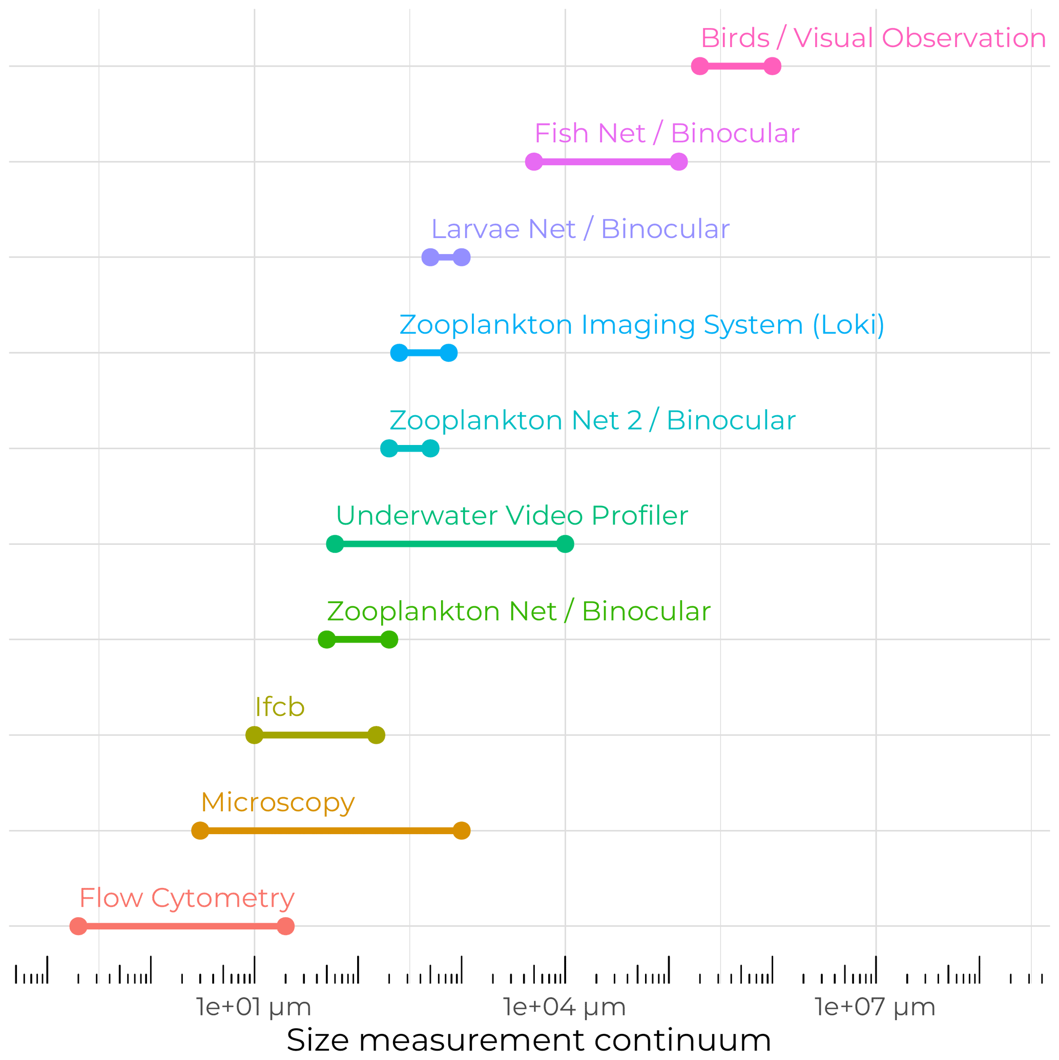
Figure 9Schematic of the biological sampling size continuum across the various methods and tools used during the Green Edge cruise.
4.5 Biodiversity
The Green Edge project also aimed to understand the related potential impacts of evolving environmental conditions on Arctic food webs in the context of climate change. Hence, great care was taken to sample the entire size spectrum of particulate matter and living organisms (Fig. 9), from the tiniest viruses and bacteria to demersal fishes, seabirds, and marine mammals. A wide variety of sampling techniques and analyses, from visual observation to highly automated underwater imaging systems, allowed us to ensure that almost all the levels of the trophic network were examined.
4.5.1 Viruses and bacteria
An abundance of viruses and bacteria was determined on fresh and preserved (glutaraldehyde 4 % final concentration) water samples taken from the rosette at each FULL and BASIC station (10 depths) using two different flow cytometers. On board, fresh samples were counted using an Accuri™ C6 and preserved samples were counted back in the lab using a FACSCanto (both machines from Becton Dickinson Biosciences, San Jose, CA, USA). Samples were processed according to Marie et al. (2001). Bacteria (and viruses) are ubiquitous in the oceans, and in Baffin Bay, we measured bacterial abundances up to 2.9×10⁶ cells mL−1.
For bacterial diversity analysis, water samples were filtered sequentially onto 20 µm, 3 µm (both polycarbonate filters, Millipore), and 0.22 µm (Sterivex-GV, Millipore). The filters and Sterivex were stored at −80 ∘C with RNAlater (Qiagen) until analyzed. The DNA/RNA co-extraction was carried out using the AllPrep DNA/RNA kit (Qiagen). The V4–V5 hypervariable region of the 16S rRNA gene was amplified by PCR using primers 515F-Y and 926R, covering a broad spectrum of diversity, including Archaea and Bacteria (Parada et al., 2016). PCR, as well as sequencing settings and bioinformatics of sequence data, can be found in Dadaglio et al. (2018).

Figure 10Relative proportions of the different microbial taxa within the different groups of samples: (a) for the 0.2–3 µm size fraction (free-living bacteria); (b) for the 3–20 µm size fraction (particle-attached bacteria); and (c) for the size fraction >20 µm (particle-attached bacteria). ICE1-2: ice stations in the transects 100 and 200; ICE3-5: ice stations in transects 300 and 500; EDGE0-18: samples between 0 and 18 m depth from the edge stations (stations 107, 204, and 312); EDGE >20: samples greater than 20 m deep from the edge stations (stations 107, 204, and 312); OWr: open water stations where the ice had receded between 2 and 8 d previously; OWo: open water stations where the ice has receded more than 15 d previously.
A comparison of the bacterial diversity as a function of geographic location and size fractions (free living bacteria, bacteria attached to particles smaller than 20 and larger than 20 µm) was made at a relatively broad taxonomic level (Fig. 10). The samples from the different groups were mainly dominated by Bacteroidetes and Proteobacteria. In general, the proportion of Proteobacteria decreased from ice stations to open-water stations featuring a more advanced stage of PSB, giving way to Bacteroidetes and, more specifically, Flavobacteriaceae.
4.5.2 Phytoplankton community
Flow cytometry was used (same protocols as for viruses and bacteria, Sect. 4.5.1) to count and differentiate the smallest cells (picophytoplankton, nanophytoplankton, cryptophytes, and Synechococcus) according to their fluorescence and scattering properties at each FULL station. At the surface, picophytoplankton and nanophytoplankton cell concentrations could reach 60 000 (station 719 – transect 7, station 19) and 9000 (station 515 – transect 5, station 15) cell mL−1, respectively, while cryptophytes were always below 360 cell mL−1. Synechococcus cyanobacteria were never observed.
Some samples were used to start phytoplankton cultures, which were taken back to the Roscoff laboratory for purification using flow cytometry sorting, serial dilution, and single-cell pipetting. Pure cultures were characterized by microscopy and 18S rRNA gene sequencing. Most cultures isolated during the cruise belonged to diatoms, especially to the genera Attheya and Chaetoceros (Gérikas Ribeiro et al., 2020). All cultures were deposited in the Roscoff Culture Collection and are available for distribution (http://www.roscoff-culture-collection.org/strains/shortlists/cruises/green-edge, last access: 19 September 2022).
To study the phytoplankton community composition, an Imaging FlowCytobot (IFCB, McLane Research Laboratories Inc., East Falmouth, MA, USA) was used during Leg 1B. The IFCB is best used for the study and identification of cells between 1 and 150 µm. Fresh samples (5 mL) taken from the rosette at each FULL station (all depths) and some BASIC and NUT stations (2 to 7 depths) were analyzed; samples from the 2 bottom-most slices of ice cores were also analyzed once melted. The IFCB takes pictures at a resolution of around 3.4 pixels per µm. Image descriptors and features were extracted with Matlab® using scripts developed by Heidi Sosik (Sosik and Olson, 2007). Taxonomic determination was achieved using Ecotaxa (Picheral et al., 2017; http://ecotaxa.obs-vlfr.fr, last access: 12 March 2022). Random forest algorithms were used for automatic classification. Reference sets and the validation of predictions were both done manually. Examples of specimens observed during the Green Edge campaigns can be found in Massicotte et al. (2020).

Figure 11Underwater Vision Profiler data. Average vertical profiles of particle concentration (per mL; a, c) and copepod volumetric fraction (cm3 m−3; b, d) at open-water (a, b) and ice-covered (c, d) stations over the top 350 m of the water column.
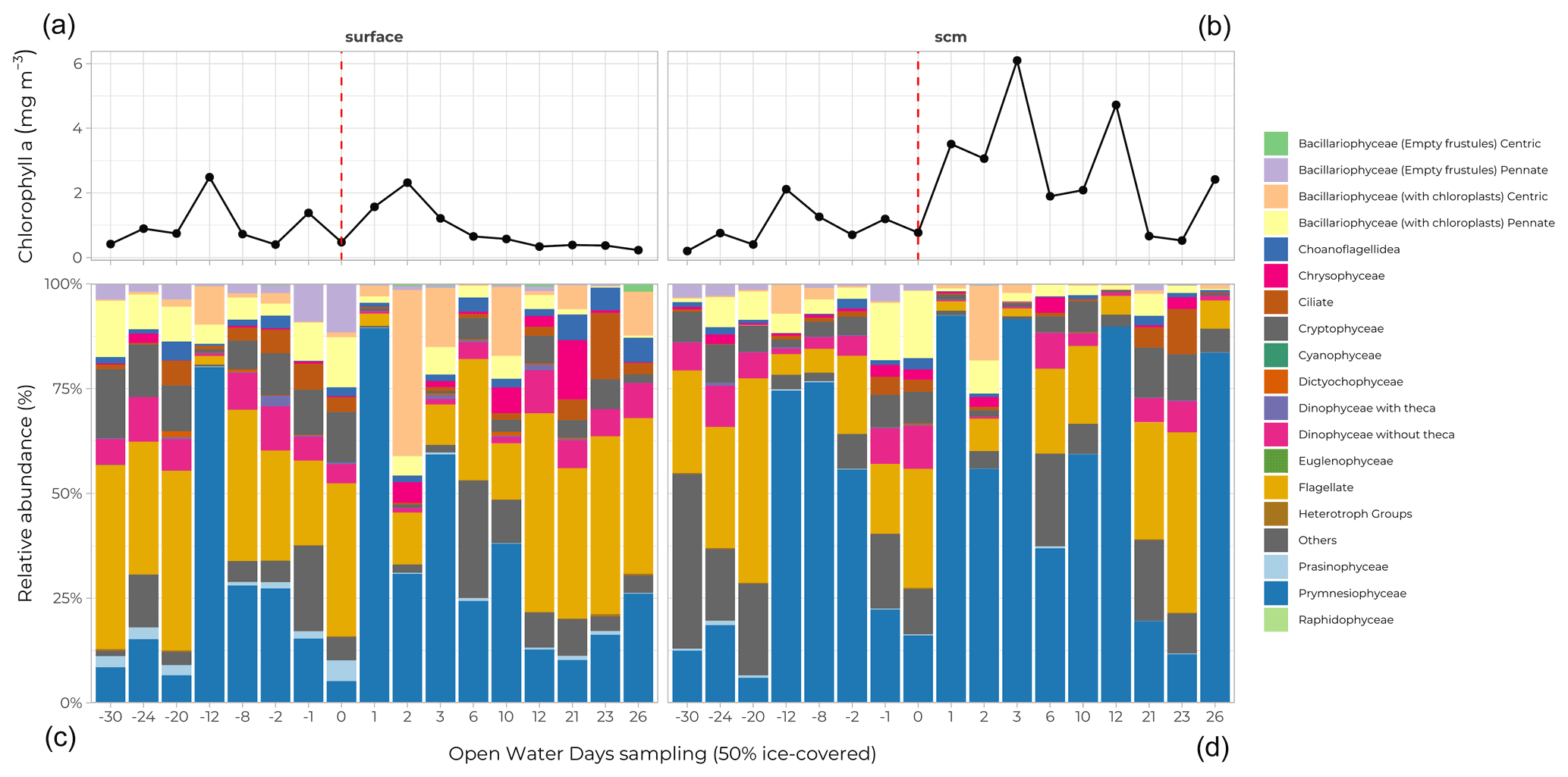
Figure 12Relative abundance (%) of main phytoplankton groups (coloured bars) at the surface (a, c) and at the subsurface chlorophyll maximum (SCM; b, d) for all stations analyzed. Stations are sorted according to their OWD value (Fig. 7); (a) and (b) represent the chlorophyll a concentration (mg m−3) at the relevant depths for each station.
A total of 203 underwater vertical profiles were acquired using an Underwater Vision Profiler (UVP, model 5-DEEP, Hydroptics, France) installed on the frame of the rosette carousel. The UVP5 collects in-focus images in the small seawater volume lit by its light emitting diodes (LEDs) as it is lowered in the water column. An automated computer system (https://ecotaxa.obs-vlfr.fr/, last access: 12 March 2022) was used to sub-sample images of individual objects and sort them into the appropriate category (marine snow or various taxa of zooplankton). The UVP has been developed mainly to count and identify particles larger than 100 µm. Figure 11 (left panels) show the average vertical profiles of particle concentration (mL−1) over the top 350 m of the water column for open-water (top) and under-ice (bottom) stations. The number of particles close to the surface in open waters coincides with the larger phytoplankton biomass observed there compared with ice-covered stations, consistent with lower primary and secondary production under sea ice. Deeper in the water column, around 300 m, the large particle concentrations observed at open-water stations likely reflect resuspension of bottom sediments, because these observations were mostly made in the eastern part of Baffin Bay over the continental shelf, whereas under-ice stations were mostly located on the deeper Canadian side of the Bay (see the bathymetry in Fig. 1).
Samples for taxonomic analyses of micro-algae by microscopy were taken at each FULL and BASIC station at 10 sampling depths. Half a litre of seawater was preserved with Lugol and kept at 4 ∘C until it was analyzed in the laboratory. Visual observation and taxonomic determination were done using an inverted microscope (Eclipse TS100, Nikon Instrument Inc.) according to the Utermöhl method (Utermöhl, 1958) using 25 or 50 mL columns. Three transects of 26 mm at 400× were systematically observed for identification and counting of Bacillariophyceae, Dinophyceae, flagellates, and ciliates. Larger phytoplankton cells and colonies were observed in all chambers at 100×. Diatoms (Bacillariophyceae) were found at every station, primarily at the surface of the water column, along with flagellates (both at the surface and in the subsurface chlorophyll maximum, SCM) (Fig. 12). The most striking feature was the dominating presence of a Phaeocystis sp. (Prymnesiophyceae, blue bars in Fig. 12) at the SCM, reaching 60 to 90 % of the cell counts (and, to a lesser extent, at the surface) across a wide range of ice cover conditions (OWD values between −12 and 12 d).
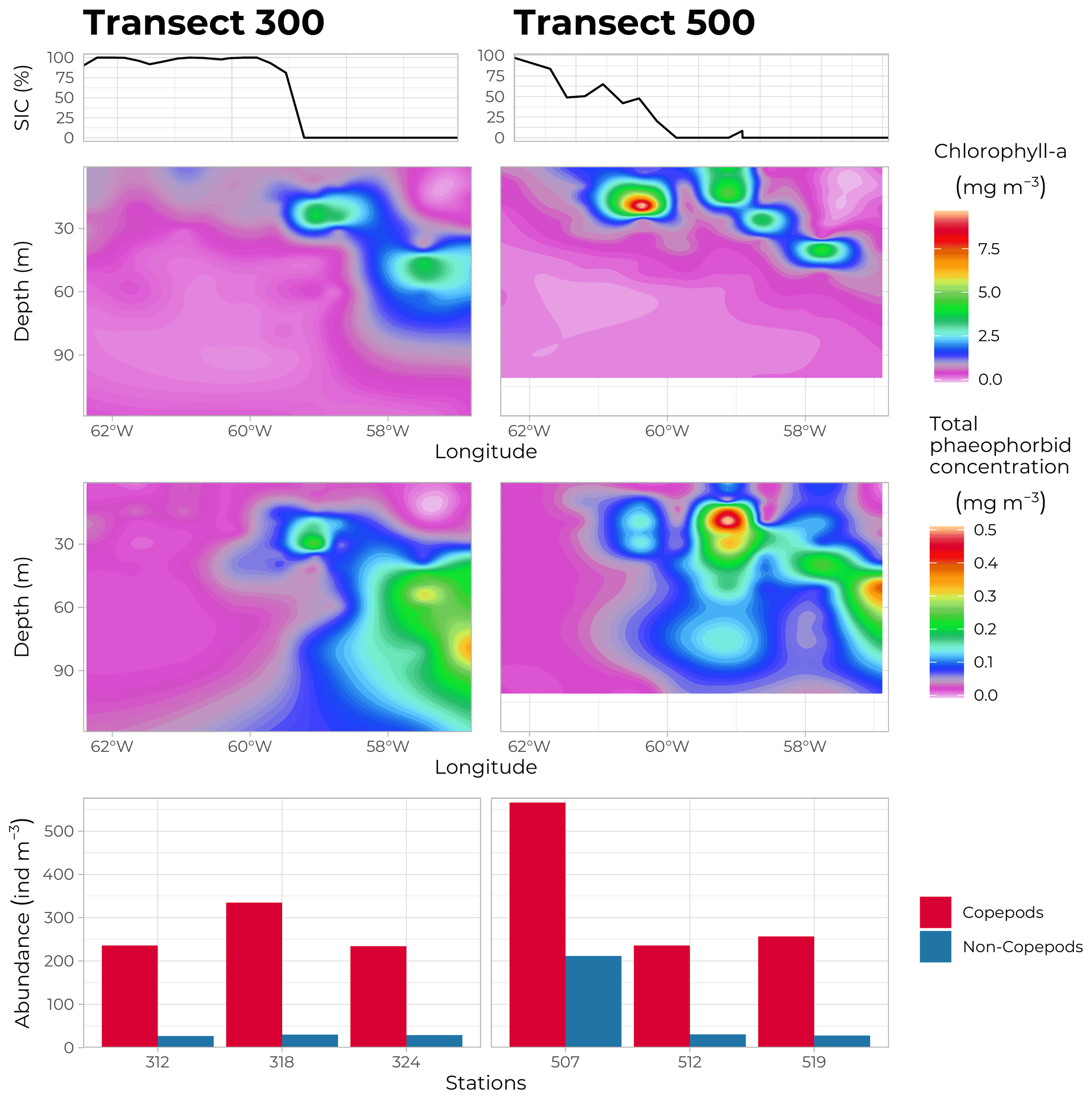
Figure 13Water column chlorophyll a concentration (mg m−3, top panels) and total phaeophorbide a concentration (mg m−3, bottom panels) along transects 300 (69∘ N, left panels) and 500 (70∘ N, right panels), as measured by HPLC on discrete samples obtained from the Niskin bottles at every FULL and BASIC station. Bottom panels: abundance of zooplankton (ind m−3), copepods in red and non-copepods in blue, at each of the three FULL stations sampled on each transect (lower station numbers towards the east). The top graphs indicate the SIC at each station at the time of sampling.
Phytoplankton and ice-algae pigments were measured to derive indices of micro-algae biomass and taxonomic composition and to get information on processes such as photoacclimation, senescence, and grazing activities (Roy et al., 2011). Rosette water samples were filtered onto GF/F filters (Whatman™, GE Healthcare Life Sciences) and quickly frozen in liquid nitrogen. Back in the land-based laboratory, samples were thawed and extracted in 100 % methanol, separated, and identified by HPLC, as described by Ras et al. (2008). A total of 25 individual pigments or groups of pigments were identified and quantified at each FULL and BASIC station (10 depths sampled each time). Figure 13 shows the distribution of total chlorophyll a and phaeophorbide concentrations along transects 300 and 500. The high chlorophyll a concentrations close to the surface in the MIZ and deepening towards open waters in the east confirmed the evolution of the PSB from an under-ice bloom to a SCM. Note that highest concentrations of phaeophorbide were systematically found underneath the accumulation of chlorophyll a, indicating the sinking of degrading phytoplanktonic material.
4.5.3 Zooplankton and fish
Zooplankton represents the second level of the food chain. The UVP5 and the Imaging FlowCytobot (see previous sections) both rendered valuable information on small zooplankton specimens (below 150 µm). Figure 11 (right panels) show copepod volumetric fraction (cm3 m−3) over the top 350 m of the water column for open-water (top panel) and under-ice (bottom panel) stations. The total copepod volumetric fraction calculated based on automatic identification made using the Ecotaxa web application (http://ecotaxa.obs-vlfr.fr, last access: 12 March 2022) shows subsurface peaks around 20 m at both open-water and ice-covered stations. A secondary peak right at the surface is present at ice-covered stations, where a subpopulation of copepods may stay close to the bottom of sea ice to feed on sympagic microalgae, small animals, and related detritus.
For bigger specimens, a series of vertical nets and trawls were deployed at each FULL station (no trawling operations took place when sea ice was present). An assembly of 4 nets of 3 different mesh sizes (50, 200 and 500 µm) coupled with a Lightframe On-sight Key species Investigation (LOKI) system rendered high-resolution pictures of individuals sampled along the water column together with actual specimens. The multi-net plankton sampler (Hydro-bios, Altenholz, Germany) uses a different sampling strategy. Composed of 9 identical nets (200 µm mesh size), it is hauled vertically in the water column, with the nets opening sequentially at different depths, each net collecting a slice of the water column displaying the vertical distribution of the species sampled. Figure 13c shows the abundance (ind m−3) of zooplankton sampled using the vertical 200 µm mesh net along transects 300 and 500. Copepods represent the main zooplankton class observed during the cruise, and they were present at every sampling site. The particularly high abundance at station 507 (situated under the ice where a phytoplankton bloom had already disappeared) might be due to the relatively high abundance of copepod nauplii (25 % of all copepod individuals compared to the usual 4 % at other stations).
Ichthyoplankton were sampled using a double square net towed obliquely from the side of the ship at a speed of ca. 2–3 knots to a maximum depth of 90 m. A Star-Oddi® mini-CTD attached to the frame and flowmeters determined the real depth and volume of sampling. For fish sampling, an echo sounder (EK60, Simrad, Kongsberg Maritime, Norway) mounted on the hull was used to locate and determine the depth of fish aggregations along the ship track during the entire cruise. When pelagic juveniles and adult fish were present at the sampling stations, an Isaac–Kidd Midwater Trawl (IKMT, Filmar and Québec-Océan, Québec, Canada) was towed for 20 min at a speed of 2–3 knots. When demersal fish were detected, a benthic beam trawl (BBT, Filmar and Québec-Océan, Québec, Canada) was used to sample bigger specimens (between 10 and 32 mm mesh size) living on the bottom sediment.
Samples of zooplankton were all processed in the same way. Swimmers (fish larvae and juveniles) were sorted out, measured, identified, and preserved in a mix of 95 % ethanol and 1 % glycerol (final concentrations) for later analysis, while zooplankton samples were preserved in 4 % formaldehyde solution. Zooplankton abundance and diversity were determined using binoculars back at the laboratory. A few samples (hydro-bios) were analyzed using the ZooScan and the Ecotaxa identification tools (https://ecotaxa.obs-vlfr.fr/prj/802, last access: 12 March 2022). Fish from IKMT and BBT sampling were sorted, counted, identified, and measured before preservation in a −20 ∘C freezer in case further analyses are needed in the future. Acoustic data from the EK60 were analyzed in Echoview® (see Geoffroy et al., 2016 for details).
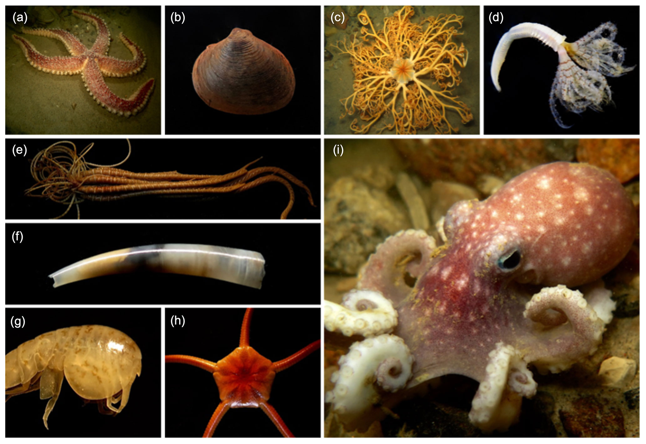
Figure 14Examples of benthic organisms. (a) Urasterias lincki, (b) Astarte borealis, (c) Gorgonocephalus eucnemis, (e) Brachiomma sp., (f) Heliometra glacialis, (g) Siphonodentalium lobatum, (h) Stegocephalus inflatus, (i) Ophiopleura borealis, Bathypolypus sp. (pictures by Benthic Ecology Lab, Université Laval, Gonzalo Bravo).
4.5.4 Benthos sampling
Benthos sampling was performed to test if (i) sea-ice cover is the primary environmental driver of the contribution and geographic distribution of sympagic carbon on the seabed, (ii) sympagic carbon is the most important baseline food source supporting benthic consumers during spring and summer in areas close to the MIZ, and (iii) deep benthic food web dynamics and structural variability are directly linked to both depth and availability of food sources (Yunda-Guarin et al., 2020). The sampling was achieved using two different strategies; a total of 16 Agassiz trawling and 34 box coring operations (some down to more than 2000 m depth) were carried out during the cruise. The Agassiz trawl (KC Denmark a/s Research Equipment) is a medium-size dredge trawled behind the ship, allowing sampling of the macrofauna living on the sediment surface. Once brought back on board, the contents of the net were immediately rinsed with seawater, manually sorted, and identified to the lowest taxonomic level possible. Samples were brought back to the laboratory to be identified under a dissecting microscope when onboard identification was impossible. Figure 14 shows an example of the diversity of benthic organisms. More than 220 species of macrofauna were identified during the Green Edge cruise from more than 25 classes (Grant, C. and Yunda-Guarin, G., unpublished data). A box corer was used to sample sediment from each FULL station. The sediment samples were then divided among the research teams for diverse analyses (see Table 3 for a complete list), including (but not limited to) identification of organisms living inside the sediment, incubations for respiration, and nutrient utilization or chemical analysis.
4.5.5 Birds and marine mammals
During the entire cruise, a systematic bird and marine mammals survey was carried out from the ship's wheelhouse (see LeBlanc et al., 2019 for detailed methodology). A total of 20 different bird species and 8 different mammal species were identified. Northern fulmar, thick-billed murre, and little auk were the most common bird species observed. Ringed seal, hooded seal, and harp seal were the most common seals. The long-finned pilot whale was the most common whale species observed. A total of 10 polar bears were observed.
A total of 123 seabirds from 7 species were also collected from a zodiac deployed from the CCGS Amundsen in Greenland waters between 10 June and 8 July. This includes black-legged kittiwakes (n=8), glaucous gulls (n=6), great black-backed gull (n=1), little auks (n=19), northern fulmars (n=42), and thick-billed murres (n=36). Sampled birds were frozen at −20 ∘C until laboratory analyses. A first study aimed to investigate the co-distribution of seabirds and their fish prey along the MIZ (LeBlanc et al., 2019). To this end, stomach contents were examined for 74 birds (35 murres, 30 fulmars, and 9 kittiwakes) under a dissecting microscope. Otoliths were retrieved and used to identify fish species, age, and size. A second focus was the recording of plastic in the stomachs. Plastic data are used in OSPAR monitoring and AMAP working groups on plastic pollution. A third study aimed to determine the birds' association to sea ice and ice-derived resources by the combination of different trophic markers. Hence, liver, muscle, and blood (from the cardiac clot) samples were collected from a total of 52 bird carcasses (27 murres, 14 auks, 3 kittiwakes, and 8 fulmars), on which highly branched isoprenoids (HBIs), carbon and nitrogen stable isotopes, and fatty acids were measured. Finally, a fourth study was looking at stable isotope data together with mercury (Hg) data for both muscle and liver.
5.1 Bacterial production, respiration, and viability
At each FULL station during the cruise, water samples were taken from 2–3 depths (surface, deep chlorophyll maximum (DCM), and below DCM) to determine bacterial respiration. Oxygen concentration was determined using the Winkler method on 1 µm filtered samples before and after a 5 d incubation in the dark at 1.5 ∘C. Bacterial respiration varied overall between 0 and 1.63 µmol O2 L−1 d−1, with a mean value of 0.35±0.41 µmol O2 L−1 d−1. For bacterial production determination, water was collected at each FULL station from 8–10 depths. Bacterial production was measured by [3H]-Leucine incorporation (Kirchman et al., 1985) modified for microcentrifugation (Smith and Azam, 1992). Overall values varied between 0 and 1.51 µgC L−1 d−1 around a mean value of 0.17±0.25 µgC L−1 d−1. The use of the propidium monoazide (PMA) method identified a high bacterial mortality in sea ice (up to 90 %) and in SPM material (up to 68 %) collected in shallower waters at station 409 and station 418 (Burot et al., 2021).
5.2 Primary production and micronutrient cycling
To determine the fate of the phytoplankton spring bloom, one must first determine primary production. In situ simulated incubations were carried out at each FULL station on water sampled from the rosette at 8–10 depths, determined as chosen percentages of surface photosynthetically available radiation (PAR, namely 100 %, 50 %, 25 %, 10 %, 6 %, 2.9 %, 1.2 %, 0.6 %, and 0.1 %). The melted bottom-most slices of ice cores were also incubated, when available. After spiking the water with a mix of tracers, samples were incubated on deck at simulated light levels identical to the sampling light levels. The dissolved and particulate matter resulting from these incubations were analyzed by mass spectrometry resulting in detailed nitrogen assimilation and regeneration values (see Table 3 for a complete list of measurements) as well as phytoplankton primary production (PP). Primary production varied between 0 and 88.13±3.0 µgC L−1 d−1 over the entire cruise.
Photosynthetic parameters also allow the calculation of primary production and provide insight into the efficiency and characteristics of the photosynthesis of a given sample. On board, photosynthetic parameters were determined by the P vs E curves method using NaH14CO-spiked incubations of water samples (Lewis and Smith, 1983). Changes in the saturation parameter Ek (µmol Quanta m−2 s−1) in the surface waters of the transect show clear variations in light level acclimation, increasing from lower values around 39 µmol Quanta m−2 s−1 at the western under-ice stations to 217 µmol Quanta m−2 s−1 at the eastern open-water stations (transect 700 values given as an example). Great emphasis was placed on the contribution of diatoms to primary production, as diatoms are the main phytoplankton group present during the PSB. Experiments on silica production and dissolution were performed throughout the cruise to locate the actively growing diatoms. These experiments confirmed the occurrence of active silicification beneath the sea ice, where both centric and pennate diatoms were observed (see details in Lafond et al., 2019).
5.3 Fate of the phytoplankton spring bloom
Some organic matter produced by the PSB was exported down the water column as algal cells aggregated and sank or were grazed upon by vertically migrating zooplankton. One ambitious experiment was conducted during the cruise to monitor the export of the PSB at a high temporal resolution. A sequential sediment trap (PPS4, Technicap, France; 12 sampling cups) was anchored to an ice floe and deployed 25 m under the ice from 15 June to 9 July 2016. Sediment trap collection cups were filled with filtered seawater adjusted to a salinity of 38 psu with NaCl and a formalin concentration of 4 % to preserve samples during deployment and after recovery. The carousel holding the sampling cups was programmed to rotate every 2 d. The sediment trap was deployed in the marginal ice zone along transect 200 (Fig. 1), eventually drifted south with the ice, and was recovered on the way back to Iqaluit. The sediment trap was no longer anchored to its floe at recovery, but sea ice was still present in the region. Taxonomic identification of the algal cells collected showed a constant export of diatoms (∼50 million cells m−2 d−1) from 15 June to early July, when a 6-fold increase in diatom fluxes was observed from 5 to 7 July (∼300 million cells m−2 d−1) along with a peak in chlorophyll a fluxes. More than half of the cells exported during the peak in algal fluxes were identified as the ice-associated pennate diatom Navicula spp. Fluxes of the ice-obligate pennate diatom Nitzschia frigida, among the first species to be consistently exported from the melting sea ice in the Arctic Ocean (Lalande et al., 2019; Dezutter et al., 2021; Nadaï et al., 2021), peaked from 23 to 25 June, probably indicating the onset of sea ice melt. Fluxes of copepod fecal pellets collected in the sediment trap were higher prior to 27 June, suggesting under-ice grazing of ice algae until the ice melted.
5.4 Benthic processes
Taken from the box corer, portions of the sediment were incubated at in situ simulated conditions of temperature and light to assess the consumption of oxygen and nutrients by endofauna. Oxygen use in the sediment cores allowed calculation of the benthic carbon demand (mgC m−2 d−1), which was found to be especially high at stations in open waters where the PSB had already reached senescence and sinking organic matter had reached the bottom.
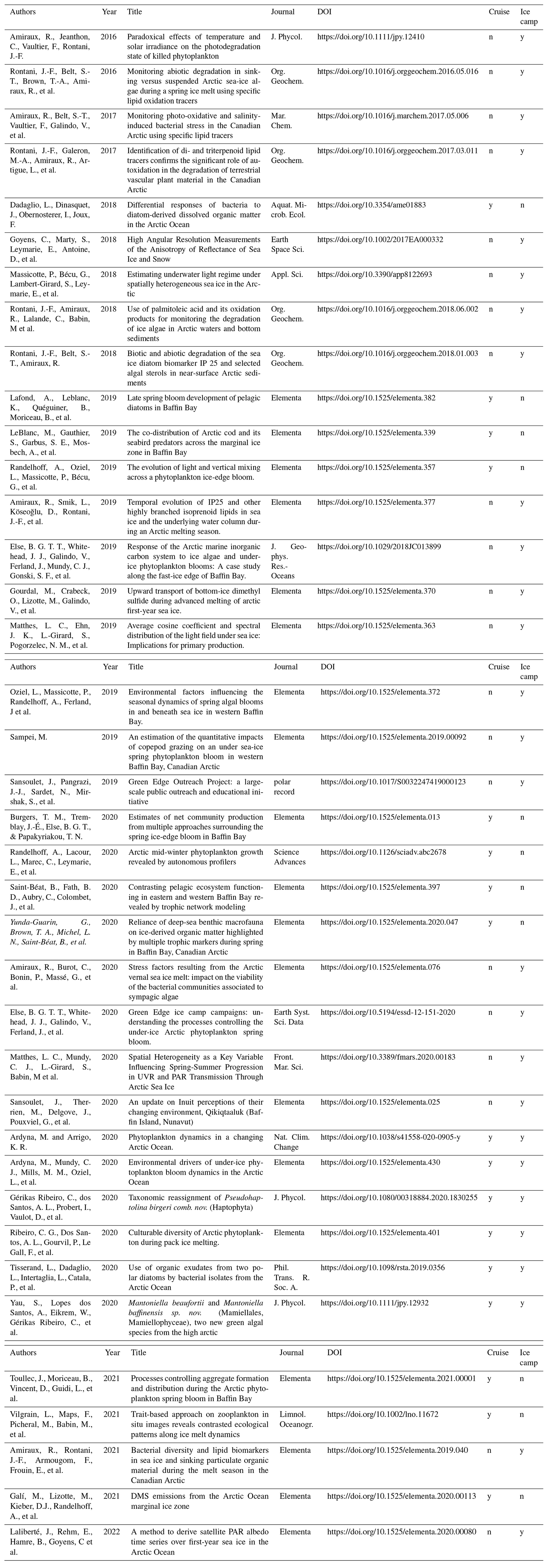
Table 5List of all peer-reviewed journal articles published so far using Green Edge cruise and/or Green Edge Ice Camp data. Only the first 4 authors are indicated in this table.
5.5 Other data
The exhaustive list of parameters measured during the cruise is presented in Table 3 along with the responsible principal investigator's (PI's) name.
Making such a large and diverse dataset available to others requires the use of many different platforms. Administrative rules and previous habits and commitments explain why our dataset is hosted by various websites, with some of it in more than one place (see in Table 3 the link and file information, when applicable for each parameter acquired during the cruise). Some funding agencies require data to be deposited in a specific database as a deliverable. In our case, the “Les Enveloppes Fluides et l'Environnement-Cycles Biogéochimiques Environnement et Ressources” (LEFE-CYBER) repository is our main host: http://www.obs-vlfr.fr/proof/php/GREENEDGE/x_datalist_1.php?xxop=greenedge&xxcamp=amundsen (last access: 29 September 2022). This is where all data and associated metadata can be found for the Green Edge cruise. Particularly, detailed metadata files associated with each variable contain the principal investigator's contact information. For specific questions, the PI associated with the data should be contacted directly. The LEFE-CYBER platform, however, does not deliver DOI, which is a very important feature for visibility of data. To obtain a DOI for the Green Edge cruise dataset (https://doi.org/10.17882/86417, Bruyant et al., 2022), we uploaded the available formatted data on SEANOE (SEA scieNtific Open data Edition) under the CC-BY license: https://www.seanoe.org/data/00752/86417 (last access: 29 September 2022). All data hosted on the SEANOE website have been formatted as described in Sect. 3, but not all the data's original formats allow transformation into the “.csv” file type. It is therefore important to keep a repository up to date where one can find all raw data.
Major long-term research programs often have their own repository/database available that has been used since the onset of their research. While the data of the BGC-Argo floats we deployed during the Green Edge cruise are hosted on the LEFE-CYBER repository, they also have been made available, together with the entire BGC-Argo dataset, from the biogeochemical Argo database: https://biogeochemical-argo.org/data-access.php (last access: 8 November 2021).
Some more specific data acquired during the cruise are also available on dedicated websites. For example, dissolved inorganic carbon (DIC), alkalinity, and 18O data are also archived with the Ocean Carbon and acidification Data System (OCADS): https://doi.org/10.25921/719e-qr37 (Miller et al., 2020).
Geographical specificity might also be a motivation for the cross-uploading of data. Since the Amundsen has been used to conduct polar research, all navigation, AVOS, ADCP, MVP, and CTD data are systematically uploaded to the Polar Data Catalog (PDC): https://www.polardata.ca/ (last access: 10 August 2022).
Please note that, in Table 3, only one address for each parameter is provided, while most of them are also available from other sources.
As for any scientific cruise, a large amount of data was acquired by many people. Even though guidelines had been suggested ahead of time for data formatting, merging, and storage, a tremendous amount of effort was necessary to collect, assemble, and standardize the data. It is important that a clear and streamlined data management plan be established ahead of time to avoid errors or loss of data in the merging process. For oceanographic CTD-rosette sampling-based cruises, depth of sampling necessitates special attention, as it is crucial to use Niskin bottle number instead of nominal depth to correctly merge the data. Furthermore, we cannot emphasize enough that data management specialists must be involved from the beginning of such large-scale projects to ensure that data is properly documented, to render the best quality dataset possible, and to avoid the loss of both valuable time and data.
The Green Edge cruise was of typical oceanographic design. In terms of goal achievement, the cruise was extremely successful and generated an impressive dataset over a diverse set of disciplines, providing a global picture of the explored environment and of all the processes fuelling the Arctic food web. Figure 4b represents all interactions existing and/or measured during the cruise between compartments of the various trophic levels. The generated dataset contains a much larger number of parameters than those presented in this paper. All data can be obtained from the data repository and provide an excellent opportunity for re-use and comparison with other Arctic datasets. A special issue of the Elementa: Science of the Anthropocene journal entitled “Green Edge – The phytoplankton spring bloom in the Arctic Ocean: past, present and future response to climate variations, and impact on carbon fluxes and the marine food web” contains a collection of research papers referring to this cruise. A complete list of peer-reviewed journal publications presenting data from either or both the Green Edge Ice Camp or Green Edge cruise can be found in Table 5.
MB designed the Green Edge project, including the scientific objectives and sampling strategy. MB, KL, FB, TL, PG, GJ, TB, MP, CM, KC, DM, MT, GD, GF, LD, JD, CL, ML, GN, NM, MC, MP, K-ML, HJ-W, ER, AV, LBdF, DD, NG, HC, AS, BQ, SH, GB, SEG, CG, P-LG, JET, EB, CS, MGT, JR, AB, RA, CB, BM, JL, EL, PB, and PC were onboard the ship and took part in sampling and onboard analysis. FB, PG, GJ, TB, MP, CM, KC, DM, MT, GD, LD, GF, LD, JD, CL, LM, GN, NM, NP, K-ML, HJ-W, ER, AV, LBdF, DD, NG, HC, AS, BG, SH, GB, GC, P-LG, M-NH, CS, MGT, JR, AB, RA, CB, BM, JL, EL, BS-B, PC, PA, LA, SB, DC, VC-B, FC, MD, CD, BE, IE, JF, LF, MG, CGR, CG, PG, CG, SH, RH, FJ, AL, PL, FLG, KL, JL, AL, ML, ALdS, GM, AM, LAM, P-IM, AM, AM, CP, MP, PR, J-FR, RS, JT, A-PT, DV, and CN took part in processing and analyzing the samples and in generating data. M-PA and PM cleaned, merged, and assembled the dataset. CS maintains the Les Enveloppes Fluides et l'Environnement-Cycles Biogéochimiques Environnement et Ressources (LEFE-CYBER) repository it is stored in. NS, SM, JS, LRL, TP and PB oversaw communication and outreach. MHF, JF, JL, and FB oversaw logistics. FB wrote the manuscript.
The contact author has declared that none of the authors has any competing interests.
Publisher's note: Copernicus Publications remains neutral with regard to jurisdictional claims in published maps and institutional affiliations.
This project was conducted using the Canadian research icebreaker CCGS Amundsen with the support of the Amundsen Science program funded by the Canada Foundation for Innovation (CFI) Major Science Initiatives (MSI) Fund. We wish to thank the officers and crew of the CCGS Amundsen. The project was conducted under the scientific coordination of the CERC on Remote Sensing of Canada's new Arctic frontier and the Centre national de la recherche scientifique CNRS/Université Laval Takuvik Joint International Laboratory (IRL3376). The field campaign was successful thanks to the contributions of Guislain Bécu, José Lagunas, Debra Christiansen-Stowe, Julie Sansoulet, Eric Rehm, Maxime Benoît-Gagné, Marie-Hélène Forget and Flavienne Bruyant, Julie Bourdon, Claudie Marec and Marc Picheral from CNRS. We also thank Québec-Océan and the Polar Continental Shelf Program for their in-kind contribution in terms of polar logistics and scientific equipment. We thank Marie-Pier Amyot for data cleaning and Étienne Ouellet for IT support and data infrastructure management. We thank Emilia Trudnowska and one anonymous referee for their numerous and useful comments.
This research has been supported by the Agence Nationale de la Recherche (ANR, grant no. 111112), the Canada Excellence Research Chair on Remote Sensing of Canada’s new Arctic Frontier (grant no. 096031), the Centre National d’Etudes Spatiales (grant no. 131425), ArcticNet (grant no. 099009), the French Arctic Initiative, Fondation Total (grant no. BIO-Février 2015-CS/036), the Canadian Space Agency (grant no. 106086), Fisheries and Ocean Canada, Sentinelle Nord (grant no. 113079), LEFE (grant no. AO2015-874272), and Institut PaulEmile Victor (IPEV, grant no. 1164).
This paper was edited by David Carlson and reviewed by Emilia Trudnowska and one anonymous referee.
André, X., Le Traon, P.-Y., Le Reste, S., Dutreuil, V., Leymarie, E., Malardé, D., Marec, C., Sagot, J., Amice, M., Babin, M., Claustre, H., David, A., D'Ortenzio, F., Kolodziejczyk, N., Lagunas, J.L., Le Menn, M., Moreau, B., Nogré, D., Penkerc'h, C., Poteau, A., Renaut, C., Schaeffer, C., Taillandier, V., and Thierry, V.: Preparing the New Phase of Argo: Technological Developments on Profiling Floats in the NAOS Project, Front. Mar. Sci., 7, 577446, https://doi.org/10.3389/fmars.2020.577446, 2020.
Antoine, D., Hooker, S. B., Bélanger, S., Matsuoka, A., and Babin, M.: Apparent optical properties of the Canadian Beaufort Sea – Part 1: Observational overview and water column relationships, Biogeosciences, 10, 4493–4509, https://doi.org/10.5194/bg-10-4493-2013, 2013.
Ardyna, M., Babin, M., Gosselin, M., Devred, E., Bélanger, S., Matsuoka, A., and Tremblay, J.-É.: Parameterization of vertical chlorophyll a in the Arctic Ocean: impact of the subsurface chlorophyll maximum on regional, seasonal, and annual primary production estimates, Biogeosciences, 10, 4383–4404, https://doi.org/10.5194/bg-10-4383-2013, 2013.
Arrigo, K. R., Perovich, D. K., Pickart, R. S., Brown, Z. W., van Dijken, G. L., Lowry, K. E., Mills, M. M., Palmer, M. A., Balch, W. M., Bates, N. R., Benitez-Nelson, C. R., Brownlee, E., Frey, K. E., Laney, S. R., Mathis, J., Matsuoka, A., Mitchell, B. G., Moore, G. W. K., Reynolds, R. A., Sosik, H. M. and Swift, J. H.: Phytoplankton blooms beneath the sea ice in the Chukchi sea, Deep-Sea Res. Pt. II, 105, 1–16, https://doi.org/10.1016/j.dsr2.2014.03.018, 2014.
Assmy, P., Fernández-Méndez, M., Duarte, P., Meyer, A., Randelhoff, A., Mundy, C. J., Olsen, L. M., Kauko, H. M., Bailey, A., Chierici, M., Cohen, L., Doulgeris, A. P., Ehn, J. K., Fransson, A., Gerland, S., Hop, H., Hudson, S. R., Hughes, N., Itkin, P., Johnsen, G., King, J. A., Koch, B. P., Koenig, Z., Kwasniewski, S., Laney, S. R., Nicolaus, M., Pavlov, A. K., Polashenski, C. M., Provost, C., Rösel, A., Sandbu, M., Spreen, G., Smedsrud, L. H., Sundfjord, A., Taskjelle, T., Tatarek, A., Wiktor, J., Wagner, P. M., Wold, A., Steen, H., and Granskog, M. A.: Leads in Arctic pack ice enable early phytoplankton blooms below snow-covered sea ice, Sci. Rep.-UK, 7, 40850, https://doi.org/10.1038/srep40850, 2017.
Atlas, R., Hoffman, R. N., Ardizzone, J., Leidner, S. M., Jusem, J. C., Smith, D. K., and Gombos, D.: A cross-calibrated, multiplatform ocean surface wind velocity product for meteorological and oceanographic applications, B. Am. Meteor. Soc., 92, 157–174, https://doi.org/10.1175/2010BAMS2946.1, 2011.
Bruyant, F., Amiraux, R., Amyot, M.-P., Archambault, P., Artigue, L., Barbedo De Freitas, L., Bécu, G., Bélanger, S., Bourgain, P., Bricaud, A., Brouard, E., Brunet, C., Burgers, T., Caleb, D., Chalut, K., Claustre, H., Cornet-Barthaux, V., Coupel, P., Cusa, M., Cusset, F., Dadaglio, L., Davelaar, M., Deslongchamps, G., Dimier, C., Dinasquet, J., Dumont, D., Else, B., Eulaers, I., Ferland, J., Filteau, G., Forget, M.-H., Fort, J., Fortier, L., Galí, M., Gallinari, M., Garbus, S.-E., Garcia, N., Gérikas Ribeiro, C., Gombault, C., Gourvil, P., Goyens, C., Grant, C., Grondin, P.-L., Guillot, P., Hillion, S., Hussherr, R., Joux, F., Joy-Warren, H., Joyal, G., Kieber, D., Lafond, A., Lagunas, J., Lajeunesse, P., Lalande, C., Larivière, J., Le Gall, F., Leblanc, K., Leblanc, M., Legras, J., Levesque, K., Lewis, K.-M., Leymarie, E., Leynaert, A., Linkowski, T., Lizotte, M., Lopes Dos Santos, A., Marec, C., Marie, D., Massé, G., Massicotte, P., Matsuoka, A., Miller, L., Mirshak, S., Morata, N., Moriceau, B., Morin, P.-I., Morisset, S., Mosbech, A., Mucci, A., Nadaï, G., Nozais, C., Obernosterer, I., Paire, T., Panagiotopoulos, C., Parenteau, M., Pelletier, N., Picheral, M., Quéguiner, B., Raimbault, P., Ras, J., Rehm, E., Ribot Lacosta, L., Rontani, J.-F., Saint-Béat, B., Sansoulet, J., Sardet, N., Schmechtig, C., Sciandra, A., Sempéré, R., Sévigny, C., Toullec, J., Tragin, M., Tremblay, J.-É., Trottier, A.-P., Vaulot, D, Vladoiu, A., Xue, L., Yunda-Guarin, G., and Babin, M.: The Green Edge cruise: following the evolution of the Arctic phytoplankton spring bloom, from ice-covered to open waters, SEANOE [data set], https://doi.org/10.17882/86417, 2022.
Burot, C., Amiraux, R., Bonin, P., Guasco, S., Babin, M., Joux, F., Marie, D., Vilgrain, L., Heipieper, H. J., and Rontani, J.-F.: Viability and stress state of bacteria associated with primary production or zooplankton-derived suspended particulate matter in summer along a transect in Baffin Bay (Arctic Ocean), Sci. Total Environ., 770, 145252, https://doi.org/10.1016/j.scitotenv.2021.145252, 2021.
Dadaglio, L., Dinasquet, J., Obernosterer, I., and Joux, F.: Differential responses of bacteria to diatom-derived dissolved organic matter in the Arctic Ocean, Aquat. Microb. Ecol., 82, 59–72, https://doi.org/10.3354/ame01883, 2018.
Dezutter, T., Lalande, C., Darnis, G., and Fortier, L.: Seasonal and interannual variability of the Queen Maud Gulf ecosystem derived from sediment trap measurements, Limnol. Oceangr., 66, S411–S426, https://doi.org/10.1002/lno.11628, 2021.
Dickson, A. G., Sabine, C. L., and Christian, J. R. (Eds.): Guide to Best Practices for Ocean CO2 measurements, PICES Special Publication 3, 191 pp., https://doi.org/10.25607/OBP-1342, 2007.
Eicken, H., Gradinger, R., Salganek, M., Shirasawa, K., Perovich, D. K., and Leppäranta, M. (Eds.): Field Techniques for Sea-Ice Research, University of Alaska Press, ISBN 1602230595, 2009.
Geoffroy, M., Majewski, A., LeBlanc, M., Gauthier, S., Walkusz, W., Reist, J. D., and Fortier, L.: Vertical segregation of age-0 and age-1+ polar cod (Boreogadus saida) over the annual cycle in the Canadian Beaufort Sea, Polar Biol., 39, 1023–1037, https://doi.org/10.1007/s00300-015-1811-z, 2016.
Gérikas Ribeiro, C., Lopes dos Santos, A., Probert, I., Vaulot, D., and Edvardsen, B.: Taxonomic reassignment of Pseudohaptolina birgeri comb. nov. (Haptophyta), Phycologia, 59, 606–615, https://doi.org/10.1080/00318884.2020.1830255, 2020.
Grasshoff, K., Kremling, K., and Ehrhardt, M. (Eds.): Methods of Seawater Analysis, Wiley-VCH, Weinheim, Germany, https://doi.org/10.1002/9783527613984, 1999.
Kirchman, D., K'nees, E., and Hodson, R.: Leucine incorporation and its potential as a measure of protein synthesis by bacteria in natural aquatic systems, Appl. Environ. Microb., 49, 599–607, https://doi.org/10.1128/aem.49.3.599-607.1985, 1985.
Lafond, A., Leblanc, K., Quéguiner, B., Moriceau, B., Leynaert, A., Cornet, V., Legras, J., Ras, J., Parenteau, M., Garcia, N., Babin, M., and Tremblay, J.-É.: Late spring bloom development of pelagic diatoms in Baffin Bay, Elementa, 7, 44, https://doi.org/10.1525/elementa.382, 2019.
Lalande, C., Nöthig, E.-M., and Fortier, L.: Algal Export in the Arctic Ocean in Times of Global Warming, Geophys. Res. Lett., 46, 5959–5967, https://doi.org/10.1029/2019GL083167, 2019.
LeBlanc, M., Gauthier, S., Garbus, S. E., Mosbech, A., and Fortier, L.: The co-distribution of Arctic cod and its seabird predators across the marginal ice zone in Baffin Bay, Elementa, 7, 1–18, https://doi.org/10.1525/elementa.339, 2019.
Letelier, R. M., Karl, D. M., Abbott, M. R., and Bidigare, R. R.: Light driven seasonal patterns of chlorophyll and nitrate in the lower euphotic zone of the North Pacific Subtropical Gyre, Limnol. Oceanogr., 49, 508–519, https://doi.org/10.4319/lo.2004.49.2.0508, 2004.
Le Traon, P.-Y., D'Ortenzio, F., Babin, M., Leymarie, E., Marec, C., Pouliquen, S., Thierry, V., Cabanes, C., Claustre, H., Desbruyères, D., Lacour, L., Lagunas, J. L., Maze, G., Mercier, H., Penkerc'h, C., Poffa, N., Poteau, A., Prieur, L., Racapé, V., Randelhoff, A., Rehm, E., Schmechtig, C. M., Taillandier, V., Wagener, T., and Xing, X.: Preparing the New Phase of Argo: Scientific Achievements of the NAOS Project, Front. Mar. Sci., 7, 577408, https://doi.org/10.3389/fmars.2020.577408, 2020.
Leu, E., Mundy, C. J., Assmy, P., Campbell, K., Gabrielsen, T. M., Gosselin, M., Juul-Pedersen, T., and Gradinger, R.: Arctic spring awakening – Steering principles behind the phenology of vernal ice algal blooms, Prog. Oceanogr., 139, 151–170, https://doi.org/10.1016/j.pocean.2015.07.012, 2015.
Lewis, M. R. and Smith, J. C.: A small volume, short-incubation-time method for measurements of photosynthesis as a function of incident irradiance, Mar. Ecol.-Prog. Ser., 13, 99–102, 1983.
Lowry, K. E., van Dijken, G. L., and Arrigo, K. R.: Evidence of under-ice phytoplankton blooms in the Chukchi Sea from 1998 to 2012, Deep-Sea Res. Pt. II, 105, 105–117, https://doi.org/10.1016/j.dsr2.2014.03.013, 2014.
Marie, D., Partensky, F., Vaulot, D., and Brussaard, C.: Enumeration of Phytoplankton, Bacteria, and Viruses in Marine Samples, Curr. Protoc. Cytom., 10, 11.11.1–11.11.15, https://doi.org/10.1002/0471142956.cy1111s10, 2001.
Massicotte, P., Amiraux, R., Amyot, M.-P., Archambault, P., Ardyna, M., Arnaud, L., Artigue, L., Aubry, C., Ayotte, P., Bécu, G., Bélanger, S., Benner, R., Bittig, H. C., Bricaud, A., Brossier, É., Bruyant, F., Chauvaud, L., Christiansen-Stowe, D., Claustre, H., Cornet-Barthaux, V., Coupel, P., Cox, C., Delaforge, A., Dezutter, T., Dimier, C., Domine, F., Dufour, F., Dufresne, C., Dumont, D., Ehn, J., Else, B., Ferland, J., Forget, M.-H., Fortier, L., Galí, M., Galindo, V., Gallinari, M., Garcia, N., Gérikas Ribeiro, C., Gourdal, M., Gourvil, P., Goyens, C., Grondin, P.-L., Guillot, P., Guilmette, C., Houssais, M.-N., Joux, F., Lacour, L., Lacour, T., Lafond, A., Lagunas, J., Lalande, C., Laliberté, J., Lambert-Girard, S., Larivière, J., Lavaud, J., LeBaron, A., Leblanc, K., Le Gall, F., Legras, J., Lemire, M., Levasseur, M., Leymarie, E., Leynaert, A., Lopes dos Santos, A., Lourenço, A., Mah, D., Marec, C., Marie, D., Martin, N., Marty, C., Marty, S., Massé, G., Matsuoka, A., Matthes, L., Moriceau, B., Muller, P.-E., Mundy, C.-J., Neukermans, G., Oziel, L., Panagiotopoulos, C., Pangrazi, J.-J., Picard, G., Picheral, M., Pinczon du Sel, F., Pogorzelec, N., Probert, I., Quéguiner, B., Raimbault, P., Ras, J., Rehm, E., Reimer, E., Rontani, J.-F., Rysgaard, S., Saint-Béat, B., Sampei, M., Sansoulet, J., Schmechtig, C., Schmidt, S., Sempéré, R., Sévigny, C., Shen, Y., Tragin, M., Tremblay, J.-É., Vaulot, D., Verin, G., Vivier, F., Vladoiu, A., Whitehead, J., and Babin, M.: Green Edge ice camp campaigns: understanding the processes controlling the under-ice Arctic phytoplankton spring bloom, Earth Syst. Sci. Data, 12, 151–176, https://doi.org/10.5194/essd-12-151-2020, 2020.
Meredith, M.,Sommerkorn, M., Cassotta, S., Derksen, C., Ekaykin, A., Hollowed, A., Kofinas, G., Mackintosh, A., Melbourne-Thomas, J., Muelbert, M. M. C., Ottersen, G., Pritchard, H., and Schuur, E. A. G.: Polar Regions, in: IPCC Special Report on the Ocean and Cryosphere in a Changing Climate, edited by: Pörtner, H.-O., Roberts, D. C., Masson-Delmotte, V., Zhai, P., Tignor, M., Poloczanska, E., Mintenbeck, K., Alegriìa, A., Nicolai, M., Okem, A., Petzold, J., Rama, B., and Weyer, N. M., https://doi.org/10.1017/9781009157964, 2019.
Miller, L. A., Davelaar, M., Caleb, D., Mucci, A., Burgers, T. M., Ahmed, M., and Irish, V.: Dissolved inorganic carbon (DIC), total alkalinity, stable oxygen isotope (O-18), temperature, salinity, dissolved oxygen and other parameters measured from discrete samples and profile observations during the Canadian Coast Guard Ship Amundsen ArcticNet cruise (EXPOCODE 18DL20160603, Leg 1 and Leg 2) in the Eastern Canadian Arctic, Baffin Bay, Nares Strait, Lancaster Sound, Barrow Strait and Coronation Gulf from 2016-06-03 to 2016-08-23 (NCEI Accession 0217304), NOAA National Centers for Environmental Information [data set], https://doi.org/10.25921/719e-qr37, 2020.
Mobley, C. D.: Estimation of the remote-sensing reflectance from above-surface measurements, Appl. Opt., 38, 7442–7455, https://doi.org/10.1364/AO.38.007442, 1999.
Mueller, J. L., Austin, R. W., Morel, A., Fargion, G. S., and McClain, C. R.: Ocean Optics Protocols For Satellite Ocean Color Sensor Validation, Revision 4. Volume 1: Introduction, Background and Conventions. Greenbelt, MD, Goddard Space Flight Space Center, 1–56, (NASA/TM-2003-21621/Rev-Vol I), https://doi.org/10.25607/OBP-61, 2003.
Mundy, C. J., Gosselin, M., Ehn, J., Gratton, Y., Rossnagel, A., Barber, D. G., Martin, J., Tremblay, J.-É., Palmer, M., Arrigo, K. R., Darnis, G., Fortier, L., Else, B., and Papakyriakou, T.: Contribution of under-ice primary production to an ice-edge upwelling phytoplankton bloom in the Canadian Beaufort Sea, Geophys. Res. Lett., 36, 1–5, https://doi.org/10.1029/2009GL038837, 2009.
Nadaï, G., Nöthig, E.-M., Fortier, L., and Lalande, C.: Early snowmelt and sea ice breakup enhance algal export in the Beaufort Sea, Prog. Oceanogr., 190, 102479, https://doi.org/10.1016/J.POCEAN.2020.102479, 2021.
Parada, A. E., Needham, D. M., and Fuhrman, J. A.: Every base matters: assessing small subunit rRNA primers for marine microbiomes with mock communities, time series and global field samples, Environ. Microbiol., 18, 1403–1414, https://doi.org/10.1111/1462-2920.13023, 2016.
Perrette, M., Yool, A., Quartly, G. D., and Popova, E. E.: Near-ubiquity of ice-edge blooms in the Arctic, Biogeosciences, 8, 515–524, https://doi.org/10.5194/bg-8-515-2011, 2011.
Picheral, M., Colin, S., and Irisson, J.-O.: EcoTaxa, a tool for the taxonomic classification of images, http://ecotaxa.obs-vlfr.fr (last access: 2 December 2019), 2017.
Raimbault, P., Pouvesle, W., Diaz, F., Garcia, N., and Sempéré, R.: Wet-oxidation and automated colorimetry for simultaneous determination of organic carbon, nitrogen and phosphorus dissolved in seawater, Mar. Chem., 66, 161–169, https://doi.org/10.1016/S0304-4203(99)00038-9, 1999.
Randelhoff, A., Oziel, L., Massicotte, P., Bécu, G., Galí, M., Lacour, L., Dumont, D., Vladoiu, A., Marec, C., Bruyant, F., Houssais, M.-N., Tremblay, J.-É., Deslongchamps, G., and Babin, M.: The evolution of light and vertical mixing across a phytoplankton ice-edge bloom, Elementa, 7, 20, https://doi.org/10.1525/elementa.357, 2019.
Ras, J., Claustre, H., and Uitz, J.: Spatial variability of phytoplankton pigment distributions in the Subtropical South Pacific Ocean: comparison between in situ and predicted data, Biogeosciences, 5, 353–369, https://doi.org/10.5194/bg-5-353-2008, 2008.
Röttgers, R. and Gehnke, S.: Measurement of light absorption by aquatic particles: improvement of the quantitative filter technique by use of an integrating sphere approach, Appl. Optics, 51, 1336–1351, https://doi.org/10.1364/AO.51.001336, 2012.
Roy, S., Llewellyn, C. A., Egeland, E. S., and Johnsen, G. (Eds.): Phytoplankton pigments: characterization, chemotaxonomy, and applications in oceanography, Cambridge University Press, Cambridge, UK, https://doi.org/10.1017/CBO9780511732263, 2011.
Smith, D. C. and Azam, F.: A simple, economical method for measuring bacterial protein synthesis rates in seawater using 3H-leucine, Mar. microb. food webs, 6, 107–114, 1992.
Sosik, H. M. and Olson, R. J.: Automated taxonomic classification of phytoplankton sampled with imaging in-flow cytometry, Limnol. Oceanogr.-Meth., 5, 204–216, https://doi.org/10.4319/lom.2007.5.204, 2007.
Spreen, G., Kaleschke, L., and Heygster, G.: Sea ice remote sensing using AMSR-E 89-GHz channels, J. Geophys. Res.-Oceans, 113, C2, https://doi.org/10.1029/2005JC003384, 2008.
Stramski, D., Reynolds, R. A., Kaczmarek, S., Uitz, J., and Zheng, G.: Correction of pathlength amplification in the filter-pad technique for measurements of particulate absorption coefficient in the visible spectral region, Appl. Optics, 54, 6763–6782, https://doi.org/10.1364/ao.54.006763, 2015.
Trudnowska, E., Lacour, L., Ardyna, M., Rogge, A., Irisson, J.-O., Waite, A. M., Babin, M., and Stemmann, L.: Marine snow morphology illuminates the evolution of phytoplankton blooms and determines their subsequent vertical export, Nat. Commun., 12, 2816, https://doi.org/10.1038/s41467-021-22994-4, 2021.
U.S. National Ice Center and National Snow and Ice Data Center: compiled by: Fetterer, F., Savoie, M., Helfrich, S., and Clemente-Colón, P.: updated daily, Multisensor Analyzed Sea Ice Extent – Northern Hemisphere (MASIE-NH), Version 1. [Baffin Bay], Boulder, Colorado USA, NSIDC: National Snow and Ice Data Center, https://doi.org/10.7265/N5GT5K3K, 2010.
Utermöhl, H.: Zur Vervollkommnung der Quantitativen Phytoplankton-Methodik, Mitt. Int. Ver. Theor. Angew. Limnol., 9, 1–38, 1958.
Wassmann, P. and Reigstad, M.: Future Arctic Ocean Seasonal Ice Zones and Implications for Pelagic-Benthic Coupling, Oceanography, 24, 220–231, https://doi.org/10.5670/oceanog.2011.74, 2011.
Yunda-Guarin, G., Brown, T. A., Michel, L. N., Saint-Béat, B., Amiraux, R., Nozais, C., and Archambault, P.: Reliance of deep-sea benthic macrofauna on ice-derived organic matter highlighted by multiple trophic markers during spring in Baffin Bay, Canadian Arctic, Elementa, 8, 047, https://doi.org/10.1525/elementa.2020.047, 2020.
- Abstract
- Introduction
- Study area, sampling strategy, and ship-based operations
- Time-for-space formatting and data quality control
- Description of data collection: an overview
- Biological production and fluxes
- Data availability
- Lessons learned
- Conclusions
- Author contributions
- Competing interests
- Disclaimer
- Acknowledgements
- Financial support
- Review statement
- References