the Creative Commons Attribution 4.0 License.
the Creative Commons Attribution 4.0 License.
 | 01 Sep 2022
Airborne SnowSAR data at X and Ku bands over boreal forest, alpine and tundra snow cover
Juval Cohen
Anna Kontu
Juho Vehviläinen
Henna-Reetta Hannula
Ioanna Merkouriadi
Stefan Scheiblauer
Thomas Nagler
Elisabeth Ripper
Kelly Elder
Hans-Peter Marshall
Reinhard Fromm
Marc Adams
Joshua King
Adriano Meta
Alex Coccia
Nick Rutter
Melody Sandells
Giovanni Macelloni
Emanuele Santi
Marion Leduc-Leballeur
Richard Essery
Cecile Menard
Michael Kern
The European Space Agency SnowSAR instrument is a side-looking, dual-polarised (VV/VH), X/Ku band synthetic aperture radar (SAR), operable from various sizes of aircraft. Between 2010 and 2013, the instrument was deployed at several sites in Northern Finland, Austrian Alps and northern Canada. The purpose of the airborne campaigns was to measure the backscattering properties of snow-covered terrain to support the development of snow water equivalent retrieval techniques using SAR. SnowSAR was deployed in Sodankylä, Northern Finland, for a single flight mission in March 2011 and 12 missions at two sites (tundra and boreal forest) in the winter of 2011–2012. Over the Austrian Alps, three flight missions were performed between November 2012 and February 2013 over three sites located in different elevation zones representing a montane valley, Alpine tundra and a glacier environment. In Canada, a total of two missions were flown in March and April 2013 over sites in the Trail Valley Creek watershed, Northwest Territories, representative of the tundra snow regime. This paper introduces the airborne SAR data and coincident in situ information on land cover, vegetation and snow properties. To facilitate easy access to the data record, the datasets described here are deposited in a permanent data repository (https://doi.org/10.1594/PANGAEA.933255, Lemmetyinen et al., 2021).
- Article
(3467 KB) - Full-text XML
- BibTeX
- EndNote


The amount of water stored in seasonal snow is an essential natural resource (Sturm et al., 2017). The duration and extent of snow cover, which can be monitored with relative ease using spaceborne sensors, show notable reductions over the timescale of satellite observations (e.g. Hori et al., 2017). Modelling studies and satellite data records supported by ground observation networks have provided indications of decreasing trends in snow water equivalent (SWE) over large extents of the Northern Hemisphere (Liston and Hiemstra, 2011; Pulliainen et al., 2020). However, current satellite SWE products still lack sufficient spatial resolution and precision to meet observational requirements of many hydrological applications (Mudryk et al., 2015; Larue et al., 2017). Radar sensors operating at sufficiently high frequencies have been proposed to meet these requirements. The proposed Cold Regions Hydrology High-Resolution Observatory (CoReH2O) satellite mission aimed to retrieve SWE over land at a spatial resolution of 200–500 m at 3–15 d temporal resolution with a precision better than 3 cm for SWE ≤30 cm and better than 10 % for SWE >30 cm (Rott et al., 2010). The sensor proposed for CoReH2O was a dual polarisation synthetic aperture radar (SAR) operating at X and Ku band. While CoReH2O was not selected for mission implementation, Phase A studies motivated the acquisition and analysis of airborne radar data to advance the scientific readiness.
The European Space Agency (ESA) SnowSAR instrument is a dual-polarisation (VV, HV), airborne side-looking SAR measuring at X and Ku band (Coccia et al., 2011). Between 2010 and 2013, the instrument was operated at several sites in Northern Finland, Austrian Alps and northern Canada. The purpose of the airborne campaigns was to gather information on backscattering properties of snow-covered terrain in support of CoReH2O mission studies measuring over a range of climatological snow classes and land cover regimes. As a part of the Nordic Snow Radar Experiment (NoSREx, Lemmetyinen et al., 2016), SnowSAR was deployed in Sodankylä, Northern Finland, for a single flight in March 2011 and a total of 10 acquisition flights in the winter of 2011–2012. Two additional acquisitions took place over a tundra site near the town of Saariselkä, Finland. Three flight missions were performed between November 2012 and February 2013 in the AlpSAR campaign over three sites located in different elevation zones of the Austrian Alps representing a montane valley (Leutasch), Alpine tundra (Rotmoos) and a glacier environment (Mittelbergferner) (Rott et al., 2013). In Canada, the TVCEx campaign took place in March and April 2013 with two flight campaigns over sites in the Trail Valley Creek (TVC) watershed, Northwest Territories, representative of the tundra snow regime (King et al., 2018).
Data from SnowSAR are provided as calibrated and geocoded normalised radar cross sections (sigma-nought, σ0). At a flight altitude of 1200 m above ground, the SnowSAR swaths span approximately 400 m in ground range and up to several kilometres in the flight direction while the calibrated σ0 values are provided at spatial resolutions of 2 and 10 m. Radiometric calibration was performed by a combination of (1) internal calibration, (2) corner reflector targets installed along flight paths and (3) the application of TerraSAR-X imagery and tower-based radar observations (for cross-polarised backscatter, see Sect. 2.3). Based on repeated overpasses and cross-comparison with TerraSAR-X, the absolute accuracy at X band was determined to be better than 1 dB and the radiometric stability better than 1 dB at both X and Ku bands for 95 % of the data (Di Leo et al., 2016).
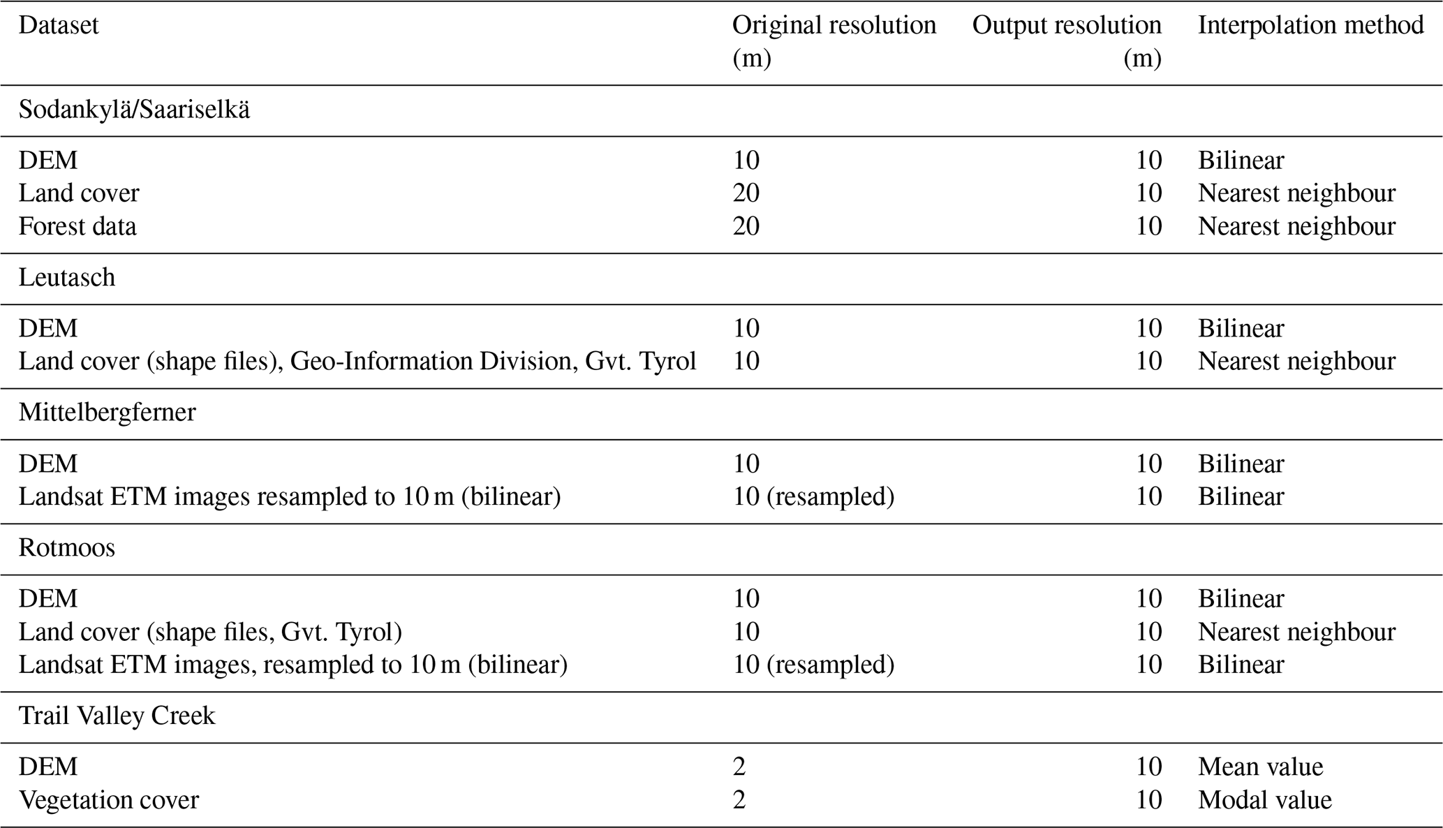
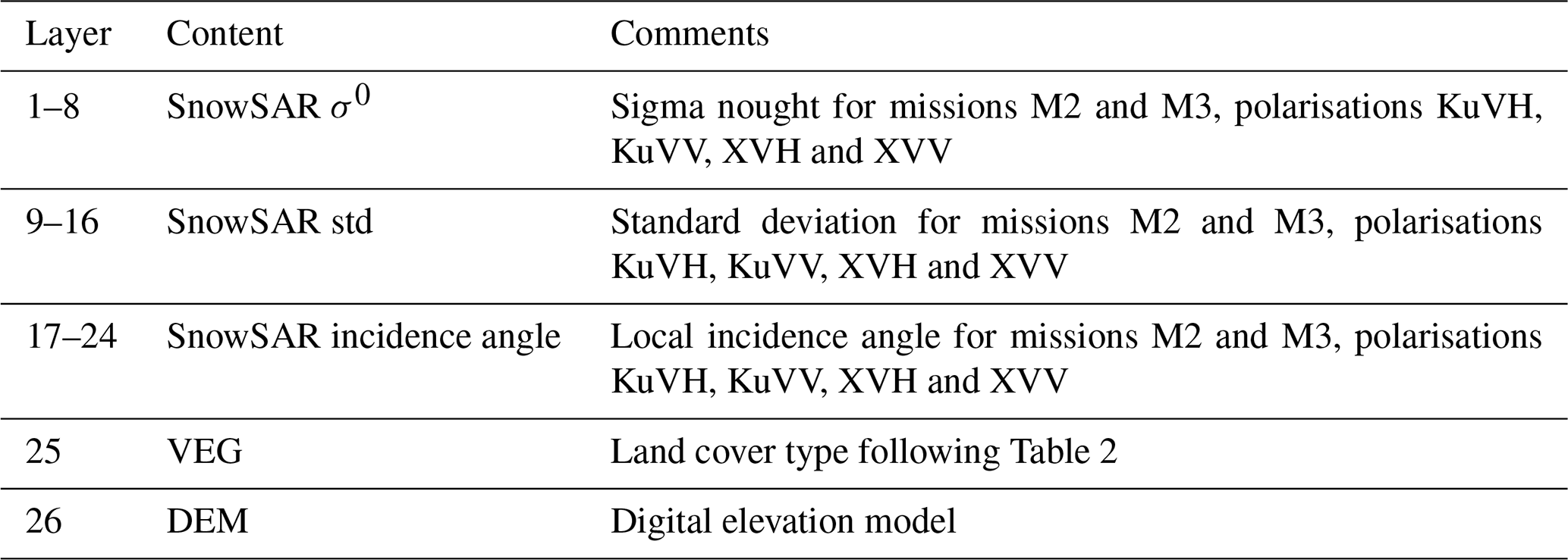
While data from individual sites have already been used in scientific studies (Cohen et al., 2015; Montomoli et al., 2016; King et al., 2018; Zhu et al., 2018; Santi et al., 2021), an effort was made here to consolidate analyses by providing both the airborne SAR acquisitions and supporting ancillary data for all sites in a common format. Consistent processing steps were applied to geocode and classify SAR data according to land cover and snow regime. Supporting information such as topography, vegetation cover and forest properties were added to the database where available. Accordingly, concurrent in situ snow and meteorological data provide means for analysis of SnowSAR backscatter variability in different environmental circumstances. To reduce sensitivity to radar speckle, increase the equivalent number of looks (ENL) and to minimise local-scale sensitivity to vegetation, all gridded data were resampled to 10 m spatial resolution; Network Common Data Form (NetCDF) data packages of SnowSAR and ancillary data were produced for each site. The main output is the classified database of observations including:
-
SnowSAR backscattering for both frequencies and co- and cross-pol channels, referred to hereafter as KuVH, KuVV, XVH and XVV;
-
SnowSAR standard deviation of original observations inside aggregated grid cells for channels – KuVH, KuVV, XVH and XVV;
-
SnowSAR local incidence angle for channels – KuVH, KuVV, XVH and XVV;
-
Ancillary data on topography (digital elevation model, DEM), vegetation/forest properties and land cover classification (depending on the availability) geocoded to the same grid as SnowSAR data;
-
In situ snow and meteorological properties (manual data collection and automated stations).
Section 2 of this article describes the SnowSAR instrument including estimated calibration accuracy. Sites, including a summary of collected SAR imagery and in situ observations, are described in Sect. 3. Data processing and the contents of the data repository are described in Sect. 4. Access to the data repository is described in Sect. 5, Sect. 6 discusses practical issues related to the use of these data and Sect. 7 provides a short summary.
2.1 System specifications
The SnowSAR instrument was developed in 2010–2011 to support Phase A studies of the CoReH2O satellite mission through simultaneous measurements of X and Ku band radar backscatter from an airborne platform. The instrument was developed by MetaSensing B.V. to emulate the anticipated observational capabilities of the CoReH2O sensor (centre frequencies, polarisation diversity) and to be operable from a small aircraft. The first version of the instrument was flown in Sodankylä, Finland, in March 2011. After the first flight, changes were made to the instrument configuration including upgraded antennas. The main characteristics of the system are summarised in Table 1.
2.2 Image processing
The processing of SnowSAR images is based on three steps:
-
range compression
-
Doppler filtering
-
ground back projection (GBP) algorithm.
Overall gain of the processing chain is calculated based on the gain/loss contribution of each of these steps. Range compression introduces a gain from performing a non-normalised fast Fourier transform being equal to the root square of the number of samples plus the windowing loss. Doppler filtering introduces further windowing loss while the GBP algorithm includes gain from range dependency correction (equal to range distance to the power of 4). The gain/loss of different processing steps is analysed in detail by DiLeo et al. (2016). This analysis shows that processing gain of SnowSAR is constant and predictable, and minimal inaccuracies are introduced during the focusing step of each pre-summed image.
2.3 Calibration and radiometric stability
Absolute calibration of SnowSAR backscattering intensity corrects for overall processing gain from the acquisition of raw data to the generation of SAR images. Besides processor and receiver gains, nominal antenna gains and constant losses in the hardware are the main contributions addressed by calibration. In practice, calibration is based on a combination of three internal and external procedures. These are briefly described in the following sections.
2.3.1 Internal calibration
An internal calibration procedure defines the noise level and receiving gain of the SnowSAR instrument. The procedure is based on (1) tracking of the transmitted power and (2) estimating the noise level during every mission. Two dedicated power metres with 0.13 dB accuracy were used to measure the transmitted power of the two radar sub-systems (X and Ku frequency bands). Transmitted power was measured through a coupler with 30 dB attenuation for X band and 27 dB for Ku band. Measured power fluctuations (relative standard deviation) within a given mission typically were in the order of 0.1 dB or less for X band and 0.25 dB for Ku band. The Finnish missions, with a total of 10 acquisitions over the site in Sodankylä, gave insight on stability of the mean transmitted power from one mission to another which varied by 1 dB for Ku band and less than 0.5 dB for X band (DiLeo et al., 2016).
Noise levels and receiving gain were estimated for each acquisition track of all SnowSAR missions directly from the range–Doppler map during the processing of the images. In practice, a section of each flight track with assumed low noise was selected. In analysing the noise variations, the XVV channel noise was found to be unstable with large variations (several dB) apparent during a given mission. The noise of all other channels exhibited stable behaviour with noise level variation less than 0.5 dB during a single mission and variations less than 1 dB from one mission to another. To compensate for the unstable behaviour of the XVV channel, a receiving gain equalisation function was applied. A reference receiving gain level was extracted from the estimated gain over the entire campaign. Then, for each acquisition track, a gain compensation factor for XVV was calculated and applied.
2.3.2 External calibration
SnowSAR external calibration, calibrating the complete observed level of the detected backscatter, compensates for antenna patterns and receiver gain contributions. Corner reflectors with a known radar cross section (RCS) were deployed at each test site. Both trihedral and dihedral corner reflectors were deployed for calibration of co- and cross-polarisation channels, respectively. However, due to the extremely narrow response of the latter in conjunction with the quite unstable motion of the small aircraft used, it was not possible to use the data of the dihedral corners and only the co-polarised channels were calibrated by using the corners. The cross-polarised data were instead calibrated using a combination of comparative TerraSAR-X imagery and tower-based radar observations (available for Finland only).
2.3.3 Radiometric stability
The radiometric stability, i.e. the capacity of the instrument to maintain a stable response to observed targets, was estimated by analysing the calibrated SAR images from repeated tracks during a given mission and by comparing sections of calibrated SAR images to the temporally closest TerraSAR-X observation available.
Calibration stability was found to vary depending on channel. There were also relatively large variations from one site to another. Table 2 summarises the calibration stability in terms of differences between repeated tracks for flights conducted at each site which indicate the level of maximum absolute difference (in dB) which covers 95 % of the observations (overlapping grid cells).
Table 2Maximum difference in SnowSAR σ0 for calibrated images of repeated tracks for selected SnowSAR missions in Sodankylä, Leutasch and TVC (from DiLeo et al., 2016).
The goal of 0.5 dB sensor stability was met for typically 85 % of all analysed data. However, the difference between calibrated σ0 on repeated tracks was less than 1 dB for 95 % of data. Further details, including a comparison with TerraSAR-X observations, are provided by Di Leo et al. (2016).
Figure 1Aerial photograph (17 March 2011) and land cover map of the Sodankylä site with planned flight transects shown. Location of weather station indicated with purple dot. Photograph courtesy of Tânia Casal, ESA.
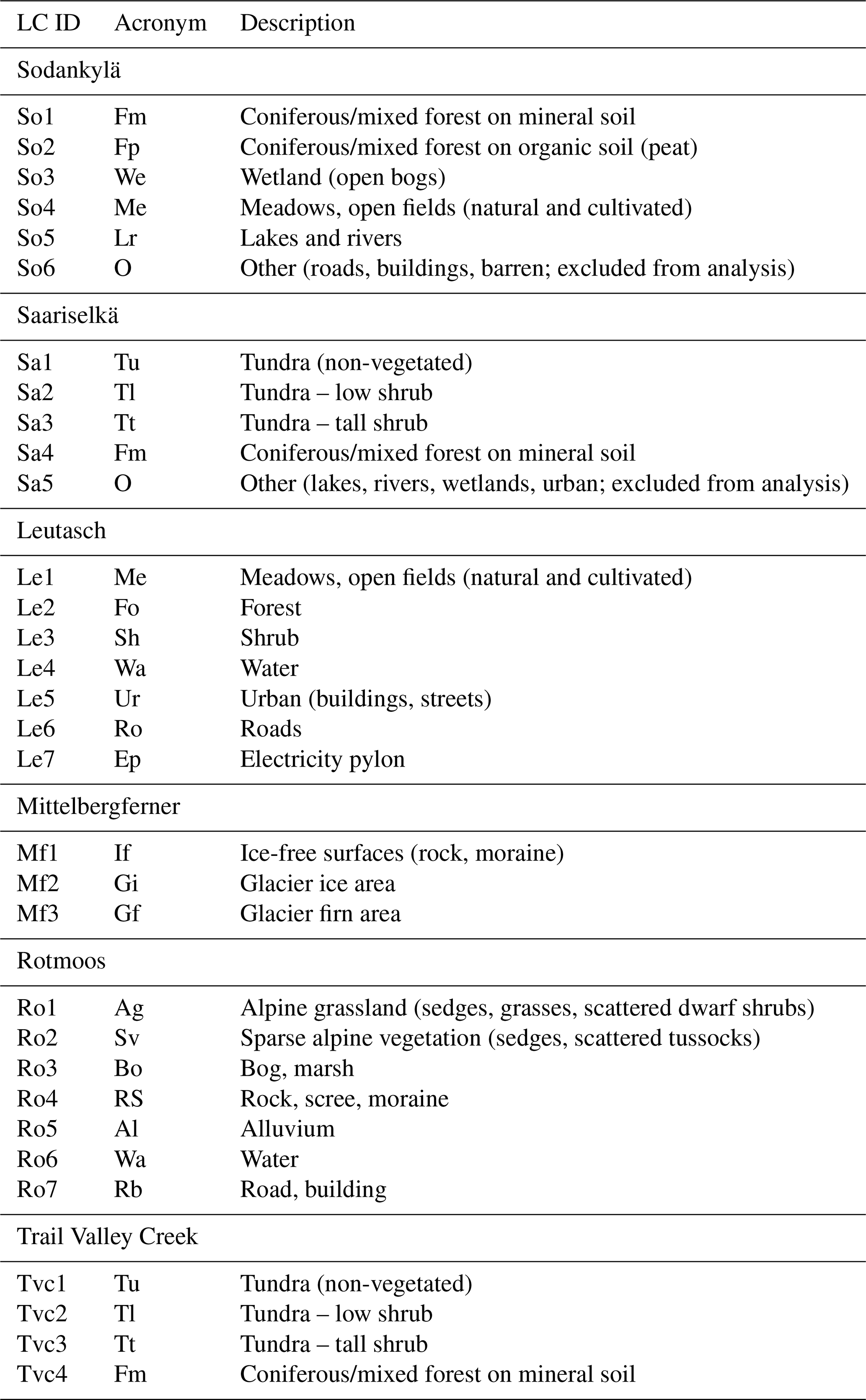
3.1 NoSREx campaigns in Finland – Sodankylä and Saariselkä
The first flight using the SnowSAR instrument took place over a boreal forest site in Sodankylä, Finland, on 17 March 2011. A total of 10 science flights were flown at the site in the following winter between December 2011 and March 2012, and an additional two flights were performed in Saariselkä, Finland, representing tundra. These flights are collectively referred to as NoSREx missions in this paper. Table 3 summarises the dates of the NoSREx missions (labelled M00 to M10 for Sodankylä and T1 to T2 for Saariselkä) and dates of the manual in situ measurements corresponding to each mission which include notes in cases where exceptions were made to co-incident snow sampling and SnowSAR data acquisitions. The details of sites, flights and collected in situ data in Finland are briefly described in the following sections.
Table 3Dates of NoSREx field campaigns, and dates and times (local time) of flight missions for the Sodankylä (Mxx) and Saariselkä (Txx) sites.

3.1.1 Sodankylä
Airborne measurements in Sodankylä covered an area of ca. 30 km2 between the town of Sodankylä and Lake Orajärvi. This taiga landscape consisted mostly of forests of varying density on mineral soil and open peatbogs (Fig. 1). Flight transects were approximately 7 km in length. A total of 25 transects were planned in a general north–south orientation and an additional two reference transects in a general east–west orientation. Measurements also covered some open fields and the westernmost end of the frozen Lake Orajärvi.
In situ data at Sodankylä included snow depth, density and snow water equivalent (SWE) measurements, snow pit observations at two fixed locations representing wetland and a forest opening, and hourly meteorological measurements. Snow depths along planned SnowSAR swaths were sampled at intervals of <10 m using the semi-automated MagnaProbe instrument (Sturm and Holmgren, 2018) or manually with a depth probe every 100 m; SWE and snow density were recorded with a coring device every 500 m (Hannula et al., 2016). Snow pit observations consisted of snow layering (stratigraphy), snow grain size, snow grain type, snow temperature profile and snow density profile (Leppänen et al., 2016).
At the Sodankylä site, not all flight transects could be sampled with in situ measurements. However, one parallel and one perpendicular transect were sampled during every campaign to provide a consistent reference. Observed snow conditions include wet/moist snow after initial accumulation, the dry snow accumulation period including snow metamorphism and the effect of melt/refreeze events in late winter.
Ancillary data on DEM and vegetation height at 2 m resolution (based on lidar scans) provided tree height, canopy cover and stem volume data at 20 m spatial resolution (Natural Resources Institute Finland, https://www.maanmittauslaitos.fi/en/maps-and-spatial-data/expert-users/product-descriptions/laser-scanning-data, last access: 27 July 2022). The high-resolution CORINE2012 database at 20 m resolution (https://www.syke.fi/projects/corine2012, last access: 27 July 2022) was used as the basis for land cover classification to the generalised classes depicted in Fig. 1 (see Sect. 4.2 for details).
3.1.2 Saariselkä
Saariselkä, ca. 150 km north of Sodankylä (Fig. 2) is a typical tundra landscape; barren rocky hills with very low vegetation cover and valleys with slightly denser low-lying vegetation but no significant forest cover. An automated weather station measuring snow depth, air and ground temperatures, and soil moisture profiles was located in the centre of the transect. A single, ca. 20 km long SAR transect was flown in this area. Sampling of snow depth and SWE at the site was conducted similarly to Sodankylä. However, no snow pit observations were made at the Saariselkä site.
Figure 2Aerial photograph (17 March 2011) and land cover map of Saariselkä with the single flight transect shown. Location of weather station indicated with purple dot. Photograph courtesy of Tânia Casal, ESA.
The two missions flown over Saariselkä cover initial accumulation of (dry) snow and then late winter conditions with wind-controlled redistribution and densification typical for tundra snow. DEM, lidar and land cover data from Saariselkä are identical to those available for Sodankylä.
3.1.3 SAR imagery
Airborne data acquisitions were planned to follow a 15 d repeat period between December and mid-February corresponding to the repeat–pass time of the second phase of the proposed CoReH2O mission. Between 22 February and 9 March, a 3 d repeat period was planned corresponding to the repeat–pass time during the first phase of CoReH2O. A total of 10 flights were flown at Sodankylä and two flights over Saariselkä. Figure 3 shows example images of Ku band VV backscatter collected over the Sodankylä and Saariselkä sites) exemplifying the variability of backscattering with land cover, snow conditions and topography. For example, in Sodankylä, relatively low backscatter (−10 to −12 dB) is observed over wetlands while forested areas exhibit backscattering between −8 and −6 dB.

Figure 3Examples of measured KuVV backscatter swath mosaics (in dB) over Sodankylä and Saariselkä, Finland, during the NoSREx flights M05 (Sodankylä) and T2 (Saariselkä). Location of closest weather stations indicated by purple dots.
3.1.4 Meteorological and snow conditions
Figure 4 shows snow depths and air and soil temperatures measured by automated sensors at Sodankylä during the winters of 2010–2011 and 2011–2012. Snow depth information was available from acoustic depth sensors located in a forest clearing, under the forest canopy and on an open wetland (bog) (Leppänen et al., 2018). All sensors exhibited similar responses to precipitation events during both winters but the absolute magnitude of snow depths differed from one site to another with the sensor in the forest clearing exhibiting the highest depths.
The early winter season of 2010–2011 (Fig. 4, upper panel) was characterised by persistent shallow snow cover (<20 cm in the clearing) combined with temperatures remaining below freezing from 10 November onwards. This resulted in a rapid freezing of the soil due to relatively low insulation from the shallow snowpack. Snow depth increased gradually with several major precipitation events of over 10 cm from January to March. A maximum snow depth of 80 cm (ca. 170 mm in SWE) in the forest clearing was measured in March.
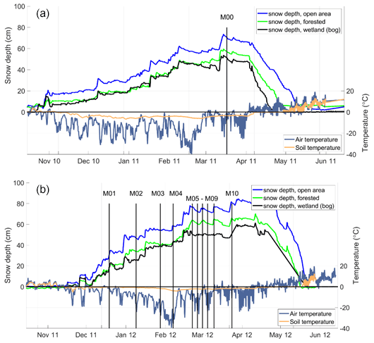
Figure 4Snow depth, air and 2 cm soil temperature at Sodankylä during 2010–2011 (a) and 2011–2012 (b) campaigns. Timing of the SnowSAR acquisitions (M00–M10) indicated with vertical lines.
Before the first SnowSAR flight on 17 March 2011 (M00), several small melt/refreeze events occurred on 3, 6 and 8 March 2011 causing densification of layers near the surface of the snowpack. No melt events were recorded during the SnowSAR flight. Measured air temperatures ranged between −14 ∘C at night to 2 ∘C during daytime (on 3 March 2011) for 1–7 March 2011 and between −8 and −1 ∘C for 17 March 2011.
Soil probes indicated a rapid freezing of soil surface layers after mid-November. Air temperatures exceeding 0 ∘C in early March did not increase measured soil moisture (not shown) suggesting that only light surface snow melt had occurred. Soil temperature measured at a depth of 2 cm and the soil moisture sensors (not shown) indicated the onset of strong snow melt only after 10 April 2011.
During the winter of 2011–2012 (Fig. 4, lower panel), the total snow depth increased from 10–30 cm during M01 to 50–80 cm during M10. The largest increase in snow depth (approximately 14–20 cm) between two consecutive SnowSAR missions occurred between M04 and M05. Soil temperature remained close to 0 ∘C until late January 2012 due to the insulating effect of the relatively deep snowpack indicating residual unfrozen water in the soil. This was also apparent in direct measurements of soil permittivity (Lemmetyinen et al., 2018).
Snow depth and air and soil temperatures at Saariselkä are presented in Fig. 5. Due to frequent high winds, the snow depth distribution is highly variable so measured depth at a single site is only an approximate measure of snow accumulation during the season. Similar to Sodankylä, soil temperatures during the first SnowSAR mission T1 were still close to 0 ∘C but the soil was frozen by T2.
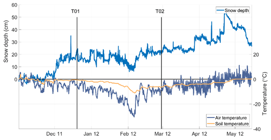
Figure 5Snow depth, air temperature and 5 cm soil temperature at Saariselkä during the winter of 2011–2012. Soil temperature from a mineral soil site at a depth of 5 cm. Timing of two SnowSAR acquisitions (T01 and T02) indicated with vertical lines.
The manual snow survey programme of the Finnish Meteorological Institute (FMI) measured snowpack evolution over two predominant land cover types in the Sodankylä region (boreal forest and wetlands; Leppänen et al., 2016). During the NoSREx flight campaigns, snow pit measurements were made coincidently with SnowSAR flight dates. Examples of manually observed snow profiles at the forest clearing site are shown in Fig. 6 for 17 March 2011 (M00) and several dates during the winter of 2011–2012. The snowpack showed a complex vertical structure during both winters, typical of the boreal forest region. The typical observed grain size in March 2011 (Fig. 6a) from macro-photography of snow samples reached 2.5–3 mm in depth hoar layers in the bottom of the snowpack. In the winter of 2011–2012, the observed grain size values were 1 to 1.5 mm throughout the winter. During M01 (b), the lower layers of the snowpack were at 0 ∘C indicating the presence of liquid water which was likely to affect observed backscatter for that date.
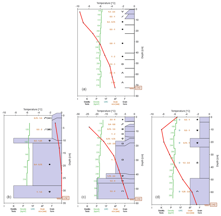
Figure 6Examples of measured snow profiles in a forest clearing site during NoSREx missions: (a) M00 (17 March 2011) and in the winter of 2011–2012, (b) M01 (19 December 2011), (c) M04 (8 February 2012) and (d) M09 (8 March 2012). Profiles include density (green line), temperature (red line), grain size (minimum–maximum ranges), grain type and hand hardness (vertical bars; K: knife, P: pencil, 1F: one finger, 4F: four fingers and F: fist). Hand hardness was not estimated on 17 March 2011.
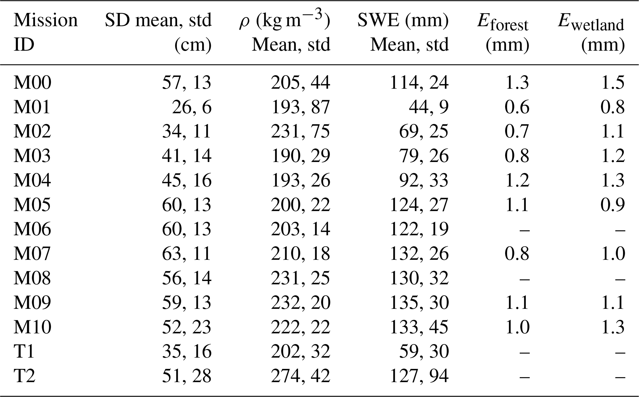
Average snow conditions (snow depth, density and SWE) measured by in situ transects are shown in Table 4. The number and location of flight transects varied per mission which may result in uncertainties when comparing one mission to another as exemplified by the apparent decrease in snow depth between M09 and M10. The average depth-weighted grain size from the two regular snow pits is also shown.
Table 4Mean and standard deviation (std) of Snow depth (SD), snow density (ρ) and SWE measured from transects during NoSREx Sodankylä missions M00–M10 and Saariselkä missions T1 and T2. Average of grain size (E) from snow pit observations on forest clearing and wetland sites (not available for M06, M08, T1 and T2).
An analysis of the time series of snow pit observations from Sodankylä in 2012 provides an indication of evolution of snowpack conditions. Figure 7 shows the bulk density (ρ) and visually estimated grain size (E) from the two weekly snow pit observations. The grain size represents a depth-weighted average over the snowpack. Both the forest clearing (Fig. 7, left) and a non-forested, open wetland (Fig. 7, right) are depicted. The dates of SnowSAR flights are indicated with vertical lines. In particular, the time series of grain size shows a relatively high degree of variability for both sites. This can be attributed to the relatively subjective method of visual estimation of grain size. The density values equally show some variability possibly due to natural spatial variability of snow (the exact location of sampling varies since the measurement is destructive). One possibility to address such issues is to perform a temporal cubic fit to the time series (as depicted) which can capture the general trend of the snow evolution.
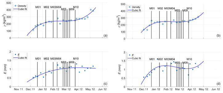
Figure 7Evolution of bulk density (ρ) and visually estimated grain size (E) from Sodankylä in the winter of 2012 from two snow pits on mineral soil (a, c) and over a wetland (b, d). Dates of SnowSAR missions identified by vertical lines. A cubic fit applied to observations depicted in blue.
3.2 Austrian Alps – AlpSAR campaign
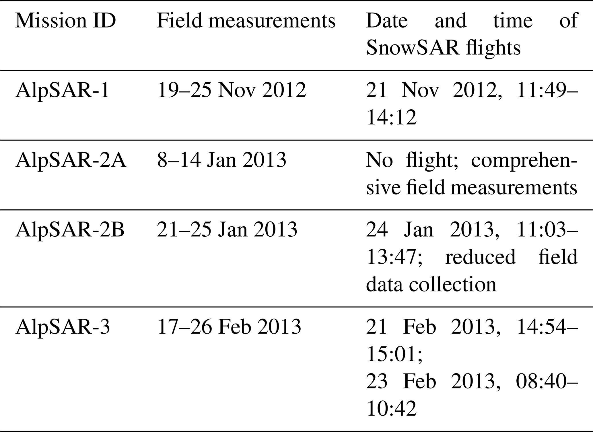
The AlpSAR 2012/13 campaign took place over three sites located in different elevation zones of the Austrian Alps. Each individual site is of limited spatial extent as the flight tracks extend along specific orographic features, i.e. narrow valleys for Leutasch and Rotmoos, respectively, and a glacier (Mittelbergferner). Consequently, differences in snowpack properties between the sites are much larger than the variability within an individual site. This is also the case for the temporal variability of processes affecting the snow metamorphic state where at the lowest site (Leutasch, elevation ca. 1150 m a.s.l.), several melt/freeze events happened during the period between the three flight campaigns whereas no melt event occurred at the two other sites (Rotmoos, ca. 2300 m a.s.l. and Mittelbergferner, 2500 to 3350 m a.s.l.). The temporal evolution of parameters of the snowpack and upper soil layers were recorded at Leutasch and Rotmoos. Time series of meteorological parameters are also available from these special stations and from nearby operational automatic stations of the Austrian Meteorological Service including a station at 2840 m elevation, 1 km from the Mittelbergferner glacier. Spatial variability in snowpack properties was measured during field campaigns coincident with the three flight missions (Table 5). An additional field campaign was conducted during the 2nd week of January 2013, scheduled to coincide with the second flight mission that was shifted due to problems with flight conditions.
Table 5Dates of the field campaigns and flight missions for AlpSAR sites.
3.2.1 Leutasch
The Leutasch valley (47.36∘ N, 11.14∘ E) extends from south-west towards north-east between the steep Wetterstein mountain range in the north and the densely forested hills of the Seefeld/Wildmoos plateau to the south. In the main data acquisition area, surface height decreases from 1158 to 1100 m a.s.l. over a horizontal distance of 5 km. Snowfall events can be intense due to orographic effects especially when frontal systems approach from the north-west. During the winter season, a network of cross-country skiing tracks runs through the valley which are visible in backscatter images as backscatter intensity is reduced due to compaction.
The land cover map (Fig. 8, right) is based on the Digital Air Photo and Lidar Atlas, Geo-information Division, Government of the Province of Tyrol. The main land cover class in the level part of the valley is meadow/fields dominated by cultivated meadows which were snow-free and in dormant stage during the first campaign in November 2012. The main forest type is dense coniferous forest which dominates the slopes but is limited in extent in the valley floor. Electricity pylons cover a very small part of the area but are included in the map because their metal frames have high radar reflectivity.
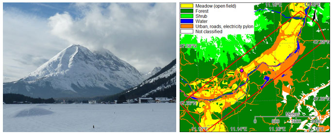
Figure 8Photograph (10 January 2013) and land cover map of Leutasch with approximate area covered by SnowSAR indicated within the red line. Location of weather station indicated by purple dot.
3.2.2 Rotmoos
The Rotmoos valley (46.82∘ N, 11.06∘ E, Fig. 9) is a small tributary to the Gurgler Tal and the Ötztaler Ache (river). The surrounding topography includes glacier-covered mountain ridges in the east, south and west reaching the highest elevation (3426 m) in the south-west corner. Snow depth and physical properties were measured in a narrow central section of the valley where the surface rises NW to SE in direction, between 2250 to 2400 m in elevation.
The Rotmoos valley is a long-term international biological and ecological monitoring site supported by the Alpine Research Centre Obergurgl of the University of Innsbruck (Koch and Erschbamer, 2010). Detailed maps on vegetation cover and geology have been aggregated into five classes (Fig. 9, right): alpine grassland, sparse alpine vegetation, bog/marsh, rock/scree/moraine and alluvium. These classes are based on the Biotope Map for Protected Areas, Digital Air Photo and Lidar Atlas, Geo-information Division, Government of Tyrol and the normalised difference vegetation index derived from top-of-atmosphere reflectance (corrected for topographic effects and atmosphere) in the ETM bands 4 (775–900 nm) and 3 (630–690 nm) of a Landsat image of 21 August 2011.
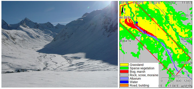
Figure 9Photograph (20 November 2012) and land cover map of the Rotmoos valley with approximate area covered by SnowSAR indicated within the red line. Location of weather station indicated by purple dot.
The upper part of the Rotmoos site is morphologically characterised by glacier foreland; the lower part and the south-west-facing slopes are mainly covered by Alpine grassland (sedges, grasses, and locally dwarf shrubs). North-east-facing slopes are steeper, covered by sparse Alpine vegetation (patchy cover of sedges). A substantial part of the level section is covered by bog including the site of the automated meteorological and snow station and of the ground-based SAR measurements (Rekioua et al., 2017). The riverbed along the valley floor is up to 100 m wide and covered by coarse material. On the orographic right side (east side) of the valley, about 1 km above the confluence with the Gurgler Ache, is a reservoir supplying water for snow production to the adjoining skiing area Obergurgl. The Rotmoos valley is a nature reserve not affected by ski pistes. During the campaigns, the snow along the flight tracks was undisturbed.
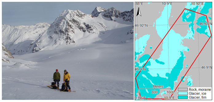
Figure 10Photograph (9 January 2013) and surface cover map of Mittelbergferner with approximate area covered by SnowSAR indicated within the red line.
3.2.3 Mittelbergferner
Mittelbergferner (46.92∘ N, 10.89∘ E, Fig. 10) is a northerly exposed glacier in the Ötztal Alps covering about 9 km2 in area over the elevation range from 2500 to 3552 m a.s.l. Field measurements were performed on the main branch of the glacier at elevations between 2700 and 3200 m. Due to warm summers during the previous two decades, the firn area was confined to north-facing slopes above about 3100 m elevation. The ice area (corresponding to exposed ice surfaces in late summer) dominates in extent over the firn area, a clear indication of negative mass balance for many years. The AlpSAR project addressed the feasibility for measuring the accumulation of seasonal snow on a glacier. At X and Ku band frequencies, the backscatter signal of the glacier during the cold period is largely dominated by the contributions of the refrozen snow and firn below the seasonal snow cover. Consequently, the state of the medium below the seasonal snow has a large impact on the backscatter behaviour. The pattern of snow accumulation during winter depends on small scale orographic effects during snowfall and on the redistribution of deposited snow due to wind. It shows a general trend of snow depth increase with elevation. The map of surface cover (Fig. 10, right) is derived from a geocoded, cloud-free Landsat image acquired on 21 August 2011. For discriminating the total glacier area versus ice-free surfaces (rock, rubble, moraine), the normalised difference snow index was used based on ETM band 5 (1550–1750 nm) and band 3. For discriminating ice and firn areas, a threshold in the top-of-atmosphere spectral reflectance image (corrected for topographic effects and atmosphere) in ETM band 4 was applied. Firn (metamorphic snow from previous years) and surfaces with remnant refrozen snow from the last winter were merged into one class (firn area) because the albedo does not allow a clear discrimination of these two sub-classes. The snow from the 2011/12 winter, not melted out during summer 2012, rested on firn so that the radar signal intensity as background to the 2012/13 winter snow is similar for both sub-classes. While there was no suitable cloudless Landsat image available in late summer 2012, an oblique aerial photo of 11 September 2012 indicated little change in the extent of glacier ice and firn areas between the two years. Measurements on firn structure at the firn temperature site (3110 m a.s.l.) show ice layers with large air bubbles between layers of compacted coarse-grained snow, being efficient scattering elements. This site is located slightly above the upper boundary of the ice area leading to the conclusion that the top firn layers were deposited as snow several years ago and had since been subject to several melt/freeze cycles.
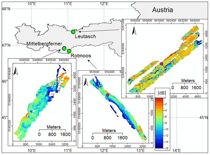
Figure 11Examples of collected KuVV SAR imagery over Mittelbergferner, Rotmoos and Leutasch during AlpSAR-3. Purple dots indicate locations of recording snow and weather stations at Rotmoos and Leutasch.
3.2.4 SAR imagery
Figure 11 gives an example of SAR data collected over the AlpSAR test sites of Leutasch, Rotmoos and Mittelbergferner. Ku band VV-pol collected on 21 and 23 February 2013 are shown. Local topography influences measurements in particular over Rotmoos and Mittelbergferner, and gaps apparent within individual tracks are mainly attributed to steep slopes. The highest backscatter values (−3 to −5 dB) were observed over the open field sites at Leutasch due to the dominant backscatter of refrozen snow. The low backscatter values at Rotmoos refer to back-slopes, but also at 40∘ angles, the backscatter intensities are lower by several dB compared to Leutasch. On Mittelbergferner, the average backscatter intensities are comparable to those of Rotmoos. Slightly higher values are observed in the firn area (in the south-east sector).
3.2.5 Meteorological and snow conditions
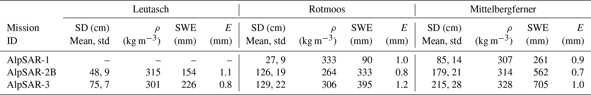
Stratigraphy and physical properties of snow (grain size and type, density profile, temperature profile) were measured in snow pits; snow depth was measured along transects using conventional techniques (depth probe) at regular intervals. Other techniques, such as the SnowMicroPen (Proksch et al., 2015), were applied to study snow characteristics but are not included in the present dataset. At Rotmoos, two experimental devices were used to map changes in snow depth: a terrestrial laser scanner and digital stereo-photography acquired from a RPAS (remotely piloted aircraft system) (Rott et al., 2013); however these data are not included here. Here, we show examples of snow pit measurements and of recorded atmosphere, snow and soil parameters. Mean values of snow depth, density and SWE collected in each of the three sites are listed in Table 6. The mean densities of the snow pits at a given site and date show only small differences. Mean SWE is computed from the mean SD of all points using the mean density of the pits.
Table 6Mean and standard deviation (std) of snow depth (SD), Density (ρ) SWE from transects. The mean density is from snow pit measurements. Mean SWE refers to the mean SD of the transects multiplied by the mean density from the snow pits. The data for Mittelbergferner refer to seasonal snow accumulating after 1 October 2012. Grain size (E) from snow pits is given as depth-weighted average of observations.
Leutasch
During the first flight campaign in Leutasch on 21 November 2012, the surface was snow-free. Accumulation of winter snow cover started on 28 November 2012 with the main build-up of the snowpack during a cold period before mid-December (Fig. 12). Between mid-December 2012 and 7 January 2013, there were three melt events, the last one with substantial rainfall which caused wetting down to the base of the snowpack. During field campaign 2A (snow pits on 10 January 2013), the lower part of the snowpack was still wet with a solid frozen crust of 10 cm thickness on top. Between 10 January and the second flight mission (24 January), the complete snowpack refroze and some fresh snow accumulated on top (field campaign 2B). The flights on 24 January and 21 February 2013 took place during cold periods when the snowpack was completely dry. Due to transient melt events before flight Mission 2, the lower 40 cm of the snowpack was composed of coarse-grained refrozen snow (grain size ranging from 1.0 to 2.5 mm) with some thin ice layers (Fig. 13). The coarse-grained layer was covered by about 10 cm of fine-grained snow during Mission 2 and by about 35 cm of fine-grained snow during Mission 3. Between Missions 2B and 3, about 75 mm SWE accumulated on the average, totalling 226 mm of SWE and a snow depth of 75 cm on 23 February 2013. The structure of the lower 40 cm of the snowpack during Mission 3 was similar to Mission 2 (coarse-grained). The snowpack above the refrozen layer was made up by several thin layers arising from sequential snowfall and short melt events with a thin top layer of fine-grained fresh snow. Snow layers above the refrozen crust were made up by rounded grains and solid faceted crystals with a grain size between 0.2 and 1.0 mm. Soil temperatures at depths of 3 and 7 cm remained above 0 ∘C throughout the snow cover period.
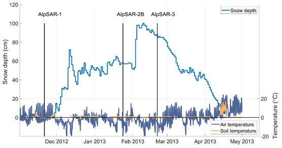
Figure 12Time series of air temperature, soil temperature (3 cm depth) and snow depth at AWS Leutasch (11.1425∘ E, 47.3708∘ N, 1135 m a.s.l.). The vertical lines indicate the dates of the three flight campaigns.
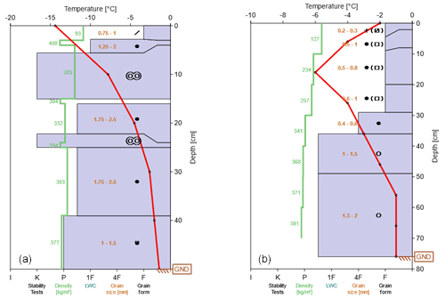
Figure 13Examples of snowpack profiles measured in Leutasch, AlpSAR campaigns 2B (a) and 3 (b) from snow pit 3.
Rotmoos
An automated station operated in the bog area at 2265 m elevation between 24 October 2012 and 27 June 2013 measuring the following variables at 5 min time steps: air temperature, humidity, pressure, wind speed and direction, and shortwave solar irradiance; snow properties: depth and temperature (20, 40, 60, 80, 100, 120 and 140 cm above ground); and soil properties: temperature and wetness (3, 11 and 30 cm below the surface). Snow depths and air and soil temperatures are presented as an example in Fig. 14.
The first snowfall event was on 27–28 October 2012 building up a snow layer of 35 cm depth. The soil below the snowpack remained unfrozen throughout winter except for the top 2 cm. There were two short melt–freeze events during the first two weeks of November. Between mid-November 2012 and mid-April 2013, no significant melt event occurred. The snowpack was completely dry during the flight missions. During the first campaign on 20–21 November, the ground was covered by 20 to 35 cm of re-frozen coarse-grained snow. The mean snow depth along the transects was 27 cm and the mean SWE was 90 mm. The coarse-grained, refrozen layer of about 30 cm depth from November stayed throughout winter with some formation of depth hoar (especially at the bog sites). Between the flight missions M1 and M2, there was one major snowfall event of about 40 cm on 28 November 2012 followed by several small events. Average snow depth increased to 126 cm and mean SWE (based on the mean density of the snow pits) to 333 mm. Between the flight missions M2 and M3, there were again some minor snowfall events. The mean snow depth increased only slightly to 129 cm whereas SWE increased to 395 mm indicating snow compaction. During M2 and M3, snow layers above the refrozen bottom layer included solid-faceted particles and also rounded grains (Fig. 15). Snow depths along the transects showed small-scale spatial variability related to micro-topography and snow redistribution by wind.
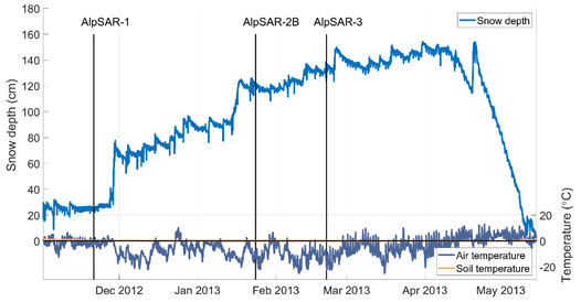
Figure 14Time series of air temperature, snow depth and soil temperature (3 cm depth) at AWS Rotmoos (11.0236∘ E, 46.8435∘ N, 2266 m a.s.l.). Vertical lines indicate the dates of the SnowSAR flight missions.
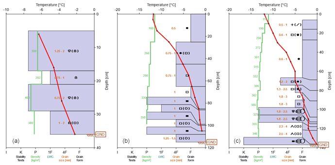
Figure 15Examples of snowpack profiles measured at Rotmoos, AlpSAR campaigns 1 and 2B from snow pit 3 (a, b) and campaign 3 from snow pit GB-SAR (near snow pit 3) (c).
Mittelbergferner
Measurements at Mittelbergferner were concerned with the feasibility of measuring seasonal snow accumulation on a temperate glacier. Snow depths and snow pit data refer to the seasonal snowpack above glacier ice or frozen firn. Measurements were made on the glacier at elevations between 2700 to 3200 m a.s.l. Up to elevations of about 3100 m, the background medium below the winter snowpack was mainly glacier ice and above about 3100 m, the background medium was frozen firn composed of coarse-grained, clustered melt–metamorphic snow with ice layers of several cm thickness. Main snowfall events after the summer melt period happened between mid-October and mid-November 2012. The snow of October was subject to melt–freeze cycles resulting in a coarse-grained bottom layer of about 30 cm thickness that persisted during winter. During Mission 1, the glacier ice and firn were already frozen down to several metres depth and were covered by a seasonal snow cover of 85 cm mean depth (mean SWE of 261 mm).
The structure and morphology of the seasonal snowpack did not change much between M1 and M3. Above the coarse-grained metamorphic base layer, several layers with fine- to medium-sized grains accumulated resulting in a mean snow depth of 2.15 m and SWE of 705 mm during M3. Due to compaction, the density increased slightly and temperature gradient metamorphism caused a minor increase in grain size through formation of faceted crystals (Fig. 16). Typical grain size of the snowpack above the basal layer ranged from 0.5 to 1.0 mm. Because the X and Ku band backscatter signal was dominated by the contributions of the frozen glacier ice, firn and bottom layer of refrozen snow, accumulation of seasonal snow with a smaller scattering albedo was associated with a slight decrease in the total backscatter coefficient.
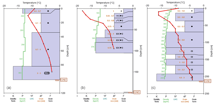
Figure 16Examples of snowpack profiles measured on Mittelbergferner, AlpSAR campaigns 1, 2A, 2B and 3 (a–d) from snow pit 4. Note that the full profile was not measured during campaign 2B (b) due to lack of time. However, snow conditions from campaign 2A (not shown) for the bottom of the snowpack can be considered valid.
3.3 Trail Valley Creek, Canada
Trail Valley Creek (TVC) is a 58 km2 research basin established in 1991 north of Inuvik, Northwest Territories, Canada (68∘45′ N, 133∘39′ W; Fig. 17). Situated near the northern edge of the boreal forest, land cover is predominantly tundra-like with isolated shrub and forest patches. Thawing of the once continuous permafrost, rapid expansion of shrub vegetation, and earlier snowmelt have contributed to substantial land cover change and ecological impact over the last 30 years (Wilcox et al., 2019; Grünberg et al., 2020). Shallow snow commonly observed within the basin (<0.3 m) is typical of a tundra environment, however, deep drifts (>2 m) form in proximity to tall standing vegetation and steep terrain (Essery and Pomeroy, 2004; King et al., 2018).

Figure 17Aerial photograph (left) and land cover map of the Trail Valley Creek (TVC) research basin overlaid by SnowSAR flight transects. Location of weather stations indicated by purple dots. Photograph courtesy of Alex Coccia, Metasensing.
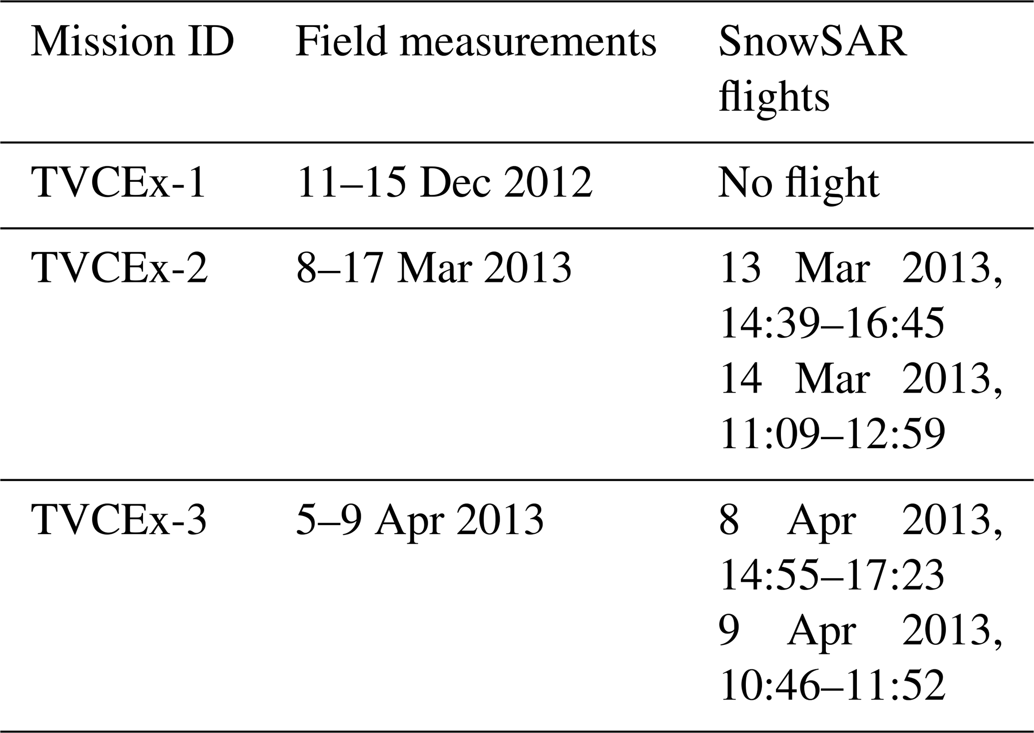
Two SnowSAR flights were performed in March and April 2013. The flight in December 2012 was cancelled; however, collection of in situ data took place (Table 7).
Table 7Dates of the field campaigns and flight missions at TVC.
The snow sampling strategy at TVC was devised to determine:
-
variability in bulk snow properties (depth, density, SWE) within and between landscape units;
-
variability in snow stratigraphic properties (layer density, grain size) within landscape units and down to the resolution of airborne radar re-sampling (∼5 to 50 m);
-
SWE stored in large drift features via ground-based lidar surveys (data not provided as part of SnowSAR dataset).
Transects of georeferenced snow depths with approximately 3 m spacing were measured using Magnaprobes throughout the research basin. More broadly spaced (∼200–500 m) ESC-30 snow core measurements provided bulk snow density measurements needed to convert Magnaprobe snow depths to SWE. Snow stratigraphic measurements were made using conventional snow pit observations (layer identification, density profiles with 100 cc cutters, visual grain dimension estimates) and objective techniques of snow specific surface area (SSA) following Gallet et al. (2009). In order to understand how stratigraphic properties measured at individual snow pits represented layer heterogeneity at the native airborne radar resolution (∼2 m), a 50 m snow trench was excavated in March and April (Rutter et al., 2019). The measurements made at each snow pit (as described above) were repeated at 5 m intervals along the trench. Near-infrared (NIR) photos along the entire trench were collected for analysis of layer (dis)continuity.
3.3.1 SAR imagery
Trail Valley Creek flight lines were surveyed during both the March and April campaign periods. Figure 18 shows a mosaic of SnowSAR swathes measured during TVCEx-2 (Ku band VV pol depicted). Distinct backscatter signatures associated with topography and vegetation were noted in the TVCEx mission data shown in Fig. 17 and the other frequency and polarisation combinations. Where roughness tussock dominated surfaces were found in valley bottom environments, increased scattering was noted at both frequencies. Additionally, outcrops of shrub vegetation throughout the domain were associated with strong scattering where interactions with the snowpack were enhanced.

Figure 18An example of SAR imagery (KuVV) over Trail Valley Creek during TVCEx-2. Location of weather stations indicated by purple dots.
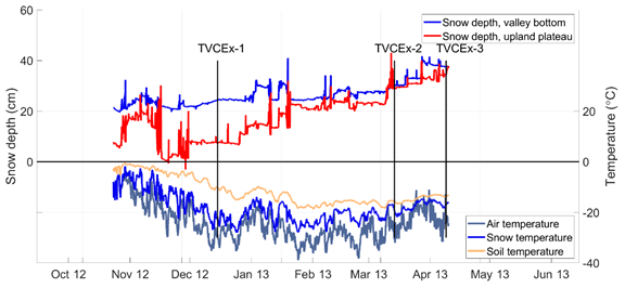
Figure 19Snow depths observed at the valley bottom and upland plateau meteorological stations within the TVC basin. Air temperature (200 cm height), snow temperature (10 cm height) and soil temperature (10 cm below surface) measured at the Upper Plateau meteorological station. Approximate date of field campaigns and SnowSAR flights indicated with vertical lines. No SnowSAR flight was performed during TVCEx-1.
3.3.2 Meteorological and snow conditions
Over the last 20 years, several meteorological stations were installed within TVC and its sub-basins. To supplement these stations, two additional sites were installed prior to the 2012/13 snow season in plateau and valley-bottom environments. Additional stations included sensors to monitor snow depth, snow temperature, soil temperature and soil permittivity. The upland plateau station (179 m a.s.l.) was located on relatively flat, gently undulating terrain covered almost entirely by graminoid tundra. The valley bottom station (104 m a.s.l.) was surrounded by steep slopes along the northern valley boundary with tall shrub tundra found on south-facing slopes and in proximity to nearby water features. Given the differences in the surrounding topography and vegetation, it was anticipated that the stations could be used to examine inter-basin differences in accumulation and snow transportation dynamics.
Figure 19 shows the seasonal progression of snow depth as observed at the upper plateau and valley bottom stations between October 2012 and April 2013 in addition to air, snow and soil temperatures at the valley bottom station. While accumulation events common to both stations were identifiable (generally observed as step changes), the snowpack at the upland tundra station eroded during the early season due to sustained exposure to prevailing northwest winds. In comparison, terrain features sheltering the valley bottom allowed retention of early season snowfall resulting in a snowpack that was over twice as deep by the December 2012 measurement campaign. A lack of standing vegetation in immediate proximity to the valley bottom station moderated overall catch efficiency and, therefore, local retention of snowfall throughout the experiment. Storm events in early January and mid-February led to small snow depth increases at the upper tundra plateau station, eventually leading to similar snow depth between the two stations by the start of the March 2013 campaign. Three small snowfall events were observed at both stations between the March and April campaigns which increased snow depth to over 30 cm by the end of the April field measurement campaigns. Wind redistribution of snow accumulation and shallow conditions observed at both stations are typical of tundra environments where snow depth in open areas is generally limited to the height of the local standing vegetation (Derksen et al., 2009).
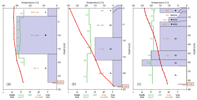
Figure 20Examples of snow pits completed near the upland tundra meteorological during sequential TVCEx field campaigns (TVCEx-1: a; TVCEx-2: c; and TVCEx-3: d).
Sustained cold air temperatures were observed at both meteorological stations throughout TVCEx. No melt events occurred with mean air temperatures well below −20 ∘C during each of the campaigns. Due to sustained cold temperatures within the snow volume, it is assumed that the radar observations were exclusively of dry snow. Soil temperatures at both stations were also found to be well below 0 ∘C (confirmed with soil pits completed at each meteorological station) and, therefore, assumed to be frozen during all observation periods. For the vast majority of the winter, temperature gradients between the snow surface and soil surface were greater than 20 ∘C m−1, strongly indicative of sustained periods of kinetic grain growth within the snow volume. In tundra environments, such conditions generally result in the development of an early season basal depth hoar layer and rapid faceting of wind slab layers (often referred to as relic or indurated wind slab, Sturm et al., 1997). Coupled with strong winds and limited precipitation, the resulting snowpack throughout the domain is generally shallow, composed of contrasting high-density wind slab and coarse-grained basal depth hoar components. Observed differences in snow depth and, therefore, the vertical temperature gradient through the snowpack also meant that strong spatial variations were evident in snow microstructure and snow layer thickness (Rutter et al., 2019).
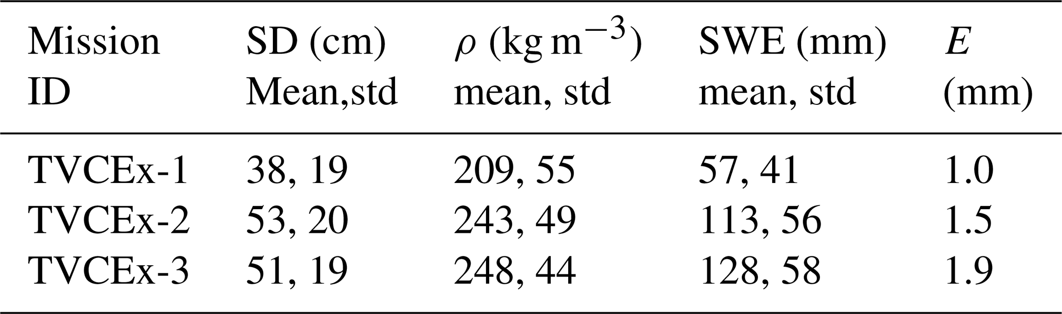
Observed snow depth and SWE from transects ranged from an average of 38 cm and 209 mm during TVCExp-1 in December 2012 to 51 cm and 248 mm in April 2013, respectively (Table 8). The variability in both snow depth and SWE was high being comparable to the Saariselkä site in Finland (Table 4).
Table 8Mean and standard deviation of snow depth, density (ρ), SWE and average grain size (E) from transects and snow pits in TVC campaigns.
Snow pits were characterised by two primary components: wind slab and basal depth hoar. The mean number of layers observed in snow pits ranged between 5 and 7 with much of the variability associated with the number of wind slab layers. Slab layers composed of fine rounded grains were a product of sustained wind events and subsequent mechanical deformation of transported crystals. Slab thickness and layering was largely governed by proximity to standing vegetation or topographic depositions whereby wind-transported snow was able to accumulate as new layers.
In the early season, depth hoar layers formed in hollows between hummocks where fresh snow was sheltered. With subsequent snowfall events, the height of open tundra depth hoar layers was found to increase with depth up to half the height of the total snowpack. Where deeper snow was found (i.e. drifts), the depth hoar layer was limited, generally comparable in thickness to layers found in shallower open tundra areas (<30 cm).
Slab layers buried by sequential snow events were not immune to kinetic growth and from an early point in the season showed signs of faceting. By April 2013, nearly the full volume of the open site snowpack was faceted (Fig. 20). By April, faceted slab layers were composed of large, well-bonded, cup-like crystals with densities similar to their previous slab form (>250 kg m−3). These layers were easily distinguished from depth hoar where basal structures were poorly bonded with much lower densities (<250 kg m−3).
4.1 SnowSAR data processing
Additional processing steps for SnowSAR data from NoSREx and TVCExp sites included calculation of Universal Transverse Mercator (UTM) coordinates and local incidence angles (xyz files) for each backscatter pixel (code by Coccia et al., 2011). These files were then processed in System for Automated Geoscientific Analyses (SAGA) (Conrad et al., 2015) where the actual geocoded images in 2 m spatial resolution and UTM projection were compiled. When re-sampling data from xyz files to the 2×2 m grids, 4 %–6 % of grid cells were left with no data, i.e. no observations were located in those grid cell areas. Correspondingly, 4 %–6 % of the grid cells had two SnowSAR observations inside one grid cell. Cells without data were filled by calculating the mean value of the surrounding eight pixels and for the grid cells with multiple measurements, the mean value of the two observations was calculated. These averaging operations during the data sampling decreased the standard deviation of the SnowSAR sigma nought observations by approximately 1 %–1.5 %.
In the case of AlpSAR, MATLAB® code provided by Metasensing (Coccia et al., 2011) was converted into Python to extract geometry information and backscatter maps from floating point data. Information from the aircraft, DEM and multilooked image files were used to receive xyz coordinates of each pixel to process the local incidence angle and sigma nought maps and project them to a 2×2 m grid. Hence, the main difference between the AlpSAR data processing method and the Sodankylä, Saariselkä and TVC processing method was in the projection of the observations to the UTM grid. For AlpSAR, the UTM coordinates of the observations were calculated from the aircraft orbit information and a DEM while for NoSREx and TVCExp, the UTM coordinates were derived from the UTM corner coordinates of the images and heading information.
For AlpSAR, the resulting backscatter maps were compared with the scaled, geocoded maps provided by Metasensing (GTiff; scaled from 8 bit to sigma nought (dB)) to verify the correct conversion with Python. For Sodankylä, Saariselkä and TVC, the image geometry was validated by comparing the resulted georeferenced grid data with other available geospatial data from the areas.
4.2 Classification based on surface type
Each SnowSAR grid cell was classified based on land cover classification (Table 9). At Sodankylä (boreal forest) and Saariselkä (tundra), land cover information from the national Finnish Corine2012 land cover database was applied (Härmä et al., 2013). Original Corine2012 classes were aggregated in order to reach the classification scheme. At TVC, land cover classification was based on an airborne lidar survey (Hopkins et al., 2011). At AlpSAR sites, land cover classification was based on public digital databases of land cover (Digitaler Laser- und Luftbildatlas Tirol, Abteilung Geoinformation, Land Tirol). At the high Alpine site Rotmoos and glacier site Mittelbergferner, the mapping of the land cover extent was further supported by terrain corrected top-of-atmosphere spectral reflectivity from geocoded Landsat images.
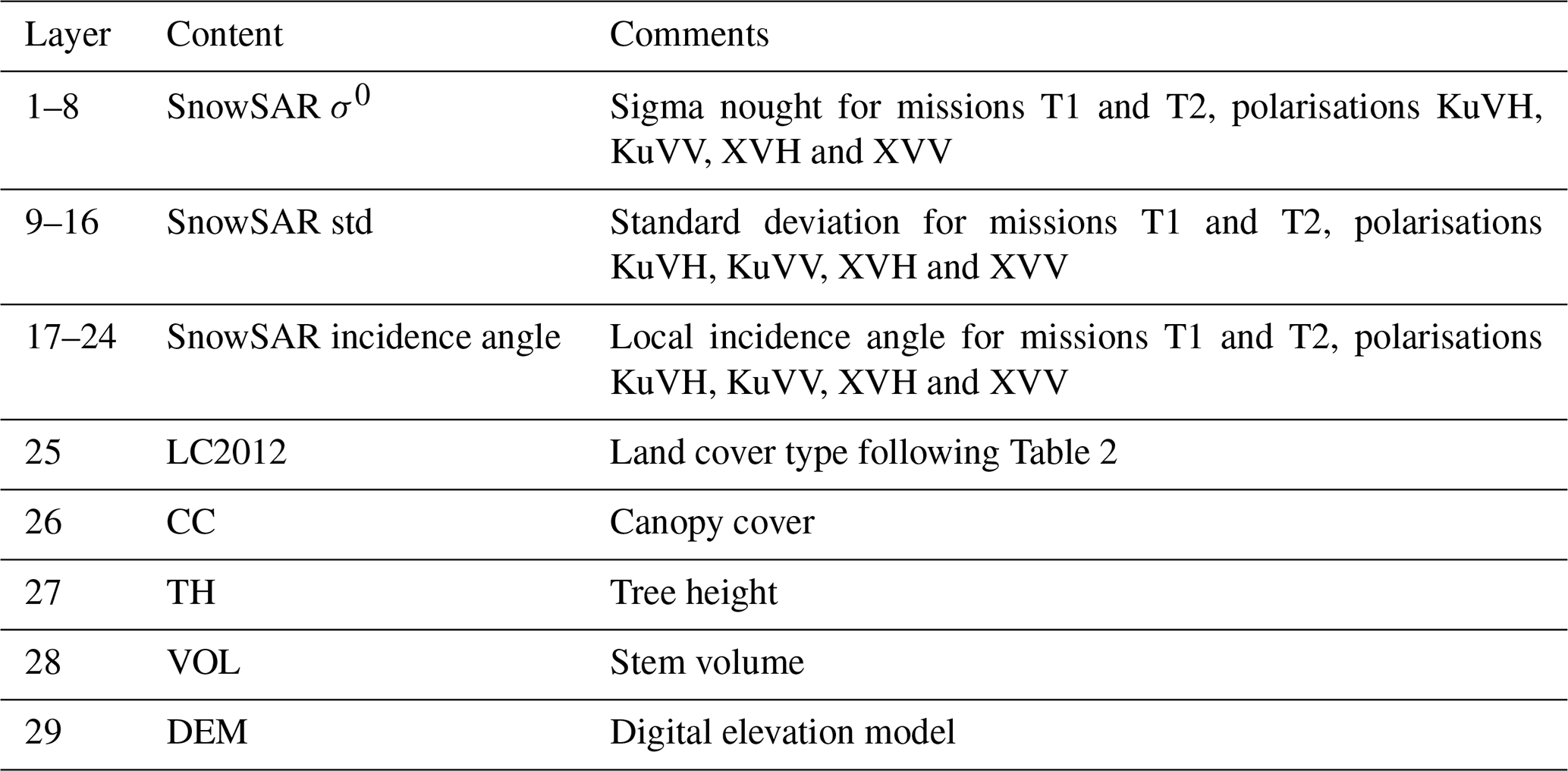
Table 13Content of structured database for AlpSAR test sites (Leutasch, Rotmoos, Mittelbergferner).

4.3 Aggregation to 10 m resolution
SnowSAR images were resampled to 10 m resolution. The values of the output grid cells (10×10 m) were the mean value of the calibrated sigma nought values (as natural numbers, not dB) in original 2×2 m grid cells. Sigma nought and local incidence angle image mosaics composed of all swaths were compiled for each mission and each polarisation. For each 10 m grid cell, the standard deviation was calculated from all SnowSAR sigma nought observations inside the grid cell. Ancillary data were resampled to the same grid as the SAR data (Table 10). A local DEM is available for each site as a separate layer resampled to the SAR grid resolution.
Table 15Summary of manual and automated datasets available from Sodankylä.

Table 16Summary of manual and automated datasets available from Saariselkä.
Table 17Summary of manual and automated datasets available from Leutasch.
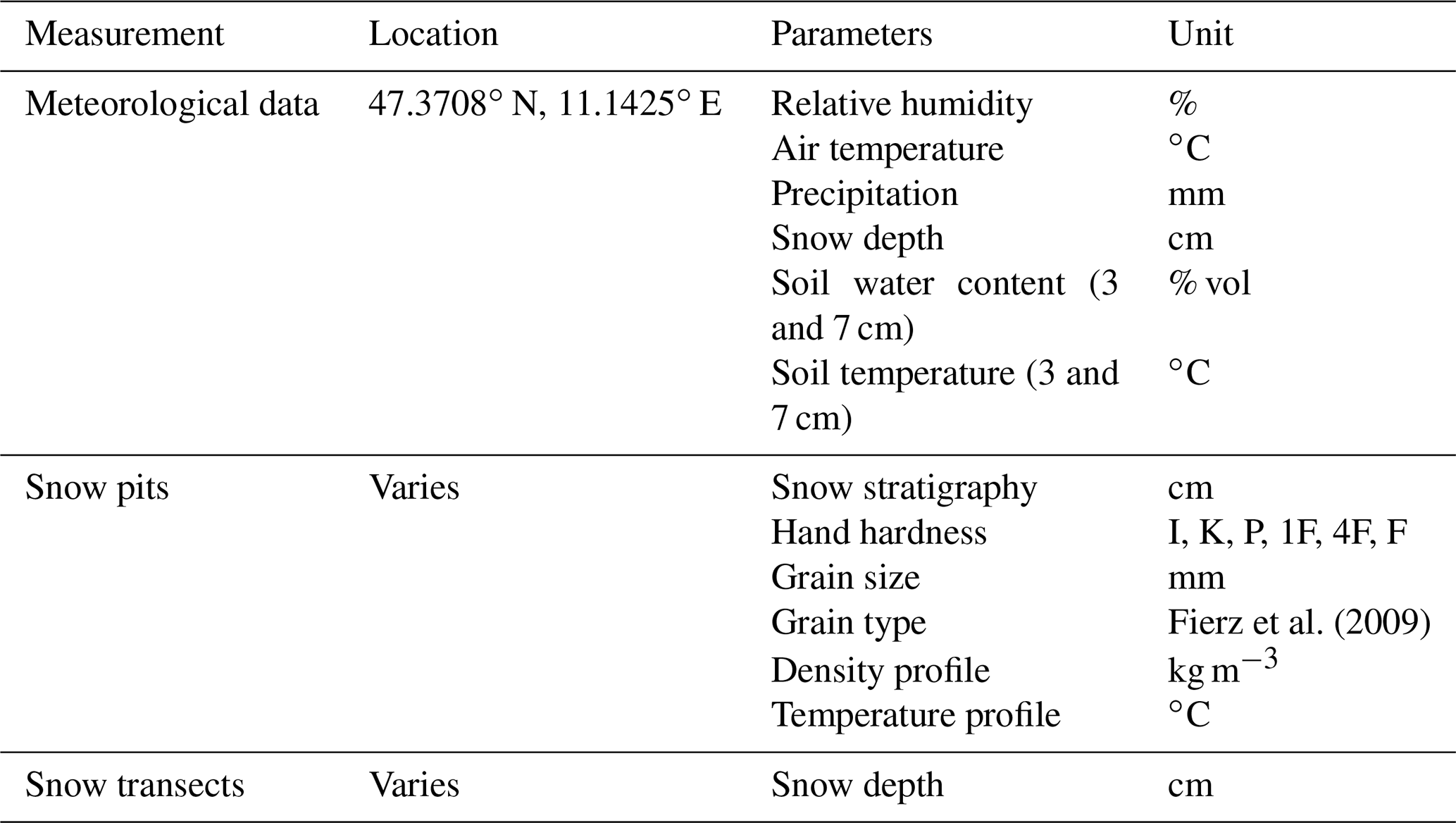
Table 18Summary of manual and automated datasets available from Rotmoos.
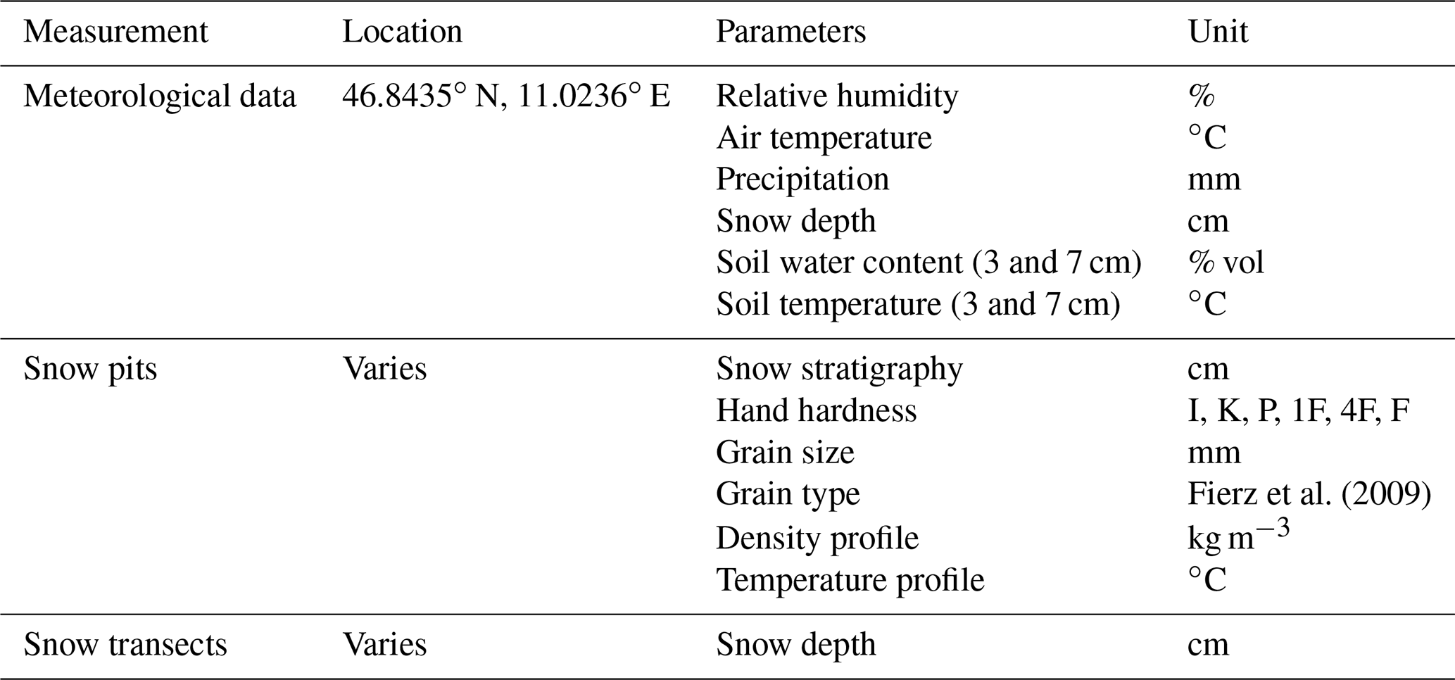
Table 19Summary of manual and automated datasets available from Mittelbergferner.
Table 20Summary of manual and automated datasets available from Trail Valley Creek.
4.4 Content of data package and data formats
4.4.1 Gridded data
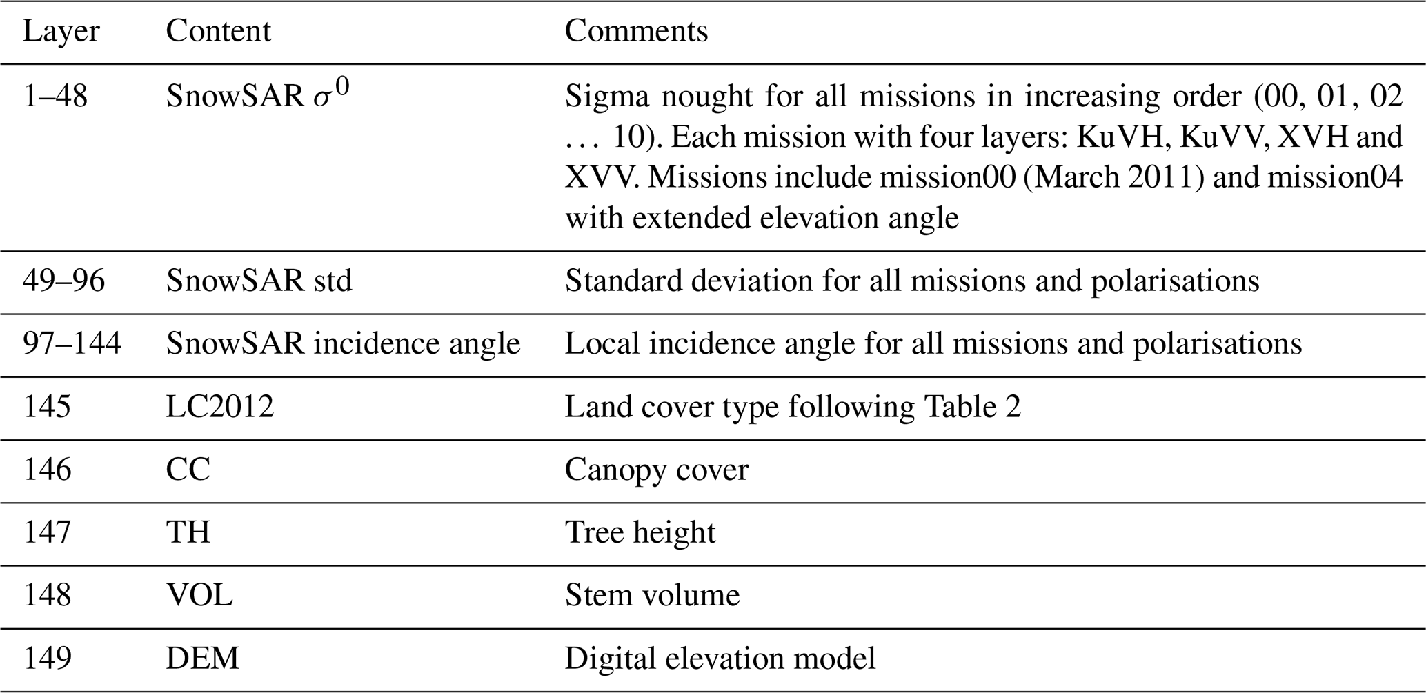
SnowSAR data are available for each site in a structured NetCDF database consisting of a layered 10 m spatial resolution geolocated matrix of: calibrated SAR backscattering intensity (sigma nought), land cover classification, DEM and vegetation/forest data. Each channel of calibrated airborne data, KuVH, KuVV, XVH and XVV (radiometric calibration provided by Metasensing), form the first layers of the dataset with calibrated sigma nought, standard deviation and local incidence angle layers corresponding to each channel. The sigma nought and incidence angle data were resampled to the relevant resolution grid (10 m) by calculating the mean value of observations inside each grid cell. Tables 11–14 describe the content of the structured database separately for all sites.
4.4.2 Meteorological and snow data
Point-based in situ measurements which could not be properly gridded such as snow depth, snow density and SWE information are available separately as vector data in ESRI shapefiles (.shp). In this format, data can be geocoded to the same coordinate reference system as the gridded database. Snow pit information is provided as annotated .xls spreadsheets in a common format (one spreadsheet for each snow profile). Weather station data are provided as .csv files; measured variables vary based on available data and are indicated in file headers. The following tables give a summary of collected in situ data at each site.
Data are available via: https://doi.org/10.1594/PANGAEA.933255 (Lemmetyinen et al. 2021). For queries regarding Sodankylä and Saariselkä data, contact Juha Lemmetyinen (juha.lemmetyinen@fmi.fi); for AlpSAR data, Helmut Rott (helmut.rott@enveo.at); and for TVC data, Chris Derken (chris.derksen@canada.ca).
Additionally, original SnowSAR data are available separately via the ESA Campaign data portal (https://doi.org/10.5270/esa-a0l50j6, Di Leo et al., 2016). Users are encouraged to contact Metasensing BV for assistance in data processing (adriano.meta@metasensing.com).
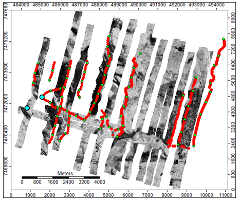
Figure 21SnowSAR X band VV pol backscatter for M02 in Sodankylä. Location of in situ snow measurements depicted with red (snow depth), green (SWE) and cyan (snow pit) dots.
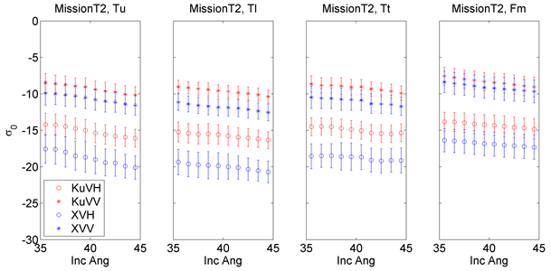
Figure 22Sensitivity of backscatter (in dB) to incidence angle during SnowSAR mission T02 for main land cover types.
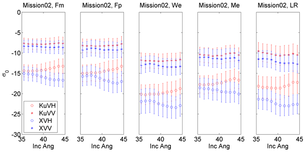
Figure 23Sensitivity of backscatter (in dB) to incidence angle during SnowSAR mission M02 for main land cover types.
6.1 Co-locating in situ observations with SnowSAR backscatter
The goal of snow measurements during SnowSAR missions was to provide a co-located reference of snow conditions to the SnowSAR swaths. For some missions, some of the snow measurements were made outside of final SnowSAR swaths due to uncertainty in aircraft navigation, the cancelling of some tracks due to limited flight time and limited swath width. Figure 21 shows an example for NoSREx M02 in Sodankylä where co-location of SnowSAR data and in situ snow measurements were poor; measurements of snow depth (red dots) and SWE (green dots) are shown against the measured XVV backscatter. Several snow measurement transects are seen to lie outside of the coverage of SnowSAR swathes making opportunities for direct comparison of backscatter with SWE and snow depth limited. However, in these cases, snow measurements can still be used as a reference for changes in snow conditions between missions, e.g. characterising different types of land cover (Hannula et al., 2016). Furthermore, physical snow models can be applied to fill spatiotemporal gaps in the SnowSAR in situ data, supporting forward modelling or retrieval studies (see e.g. Liston and Elder, 2006; Merkouriadi et al., 2021).
6.2 Effect of incidence angle
SnowSAR data are provided with an effective incidence angle relative to ground level. Due to the low flight altitudes compared to swath width, the incidence angle across-track varies more than for typical space-borne SAR instruments. To ensure proper focusing and calibration of the swaths, the nominal incidence angle range is limited from 35 to 45∘. There is still a notable effect on backscatter intensity across the swath. Figure 22 provides an example of the angular dependence of backscatter for NoSREx mission T02 at the Saariselkä test site for four land cover categories. A monotonically decreasing trend of backscattering intensity with increasing incidence angle is evident for all SnowSAR channels and most land cover types (an exception is the Tt (tundra – tall shrub) land cover class at XVH and KuVH); this type of effect can be expected for surfaces where surface scatter occurs mostly in a specular direction. However, the angular dependence is not similar for all missions or land cover types. Figure 23 depicts the angular dependence of backscatter for M02 in Sodankylä. Here, a clearly decreasing trend is only evident for the XVH channel. KuVV and XVV show no obvious change with incidence angle while the KuVH channel shows a distinct increasing trend, indicating that volume scattering could be the dominant contributor to the overall intensity of backscatter.
6.3 Lessons learnt
While being a useful tool in the development of novel remote sensing methods, airborne campaigns are relatively complex and costly. In the case of SAR, particular challenges are related to focusing and calibration. Analysis of repeated tracks during SnowSAR acquisitions determined sensor accuracy met the original goal of 0.5 dB stability for 85 % of the data (Sect. 2.3.3). In future campaigns, repeating each ground track several times during a given flight mission, as opposed to attempting to cover a large geographic area, could help to reduce uncertainties related to radiometric calibration, georeferencing and the response to variable incidence angle across the SAR swath (Figs. 22, 23). This would allow ground observations to focus on a more constrained area, also potentially avoiding instances where co-incident SAR and ground truth are unavailable due to errors in navigation or planning (Fig. 21).
Due to the relative novelty at the time, the first SnowSAR campaigns in Finland in 2011 and 2012 made only limited use of emerging tools for quantification of the snow microstructure (e.g. Domine et al., 2012; Proksch et al., 2015). While conventional snow pit observations can yield indicative information on snow microstructural evolution (e.g. Fig. 7), the more quantitative tools should be exploited comprehensively in any campaign relating snow properties to radar backscatter, as was the case for the later campaign in TVC (Rutter et al., 2019).
Snow cover in natural conditions is under constant change and airborne measurements typically capture only a few moments in time, potentially making it difficult to associate the observed parameter (e.g. radar backscatter) to properties of the evolving snowpack. The SnowSAR measurements from Finland in 2011 and 2012 can also be applied together with tower-based observations made at Sodankylä (Lemmetyinen et al., 2016). For any future campaign, a similar ground-based remote sensing component would be recommended to fill in the temporal observation gap of typical airborne operations.
With the exception of Leutasch for AlpSAR-1, deployment of SnowSAR was too late for capturing a snow-free scene (despite best efforts). This poses a problem for testing e.g. the CoReH2O retrieval approach which compares backscatter from snow cover to an earlier snow-free surface. When testing potential retrieval approaches for other sites than Leutasch, users may have to resort to simulations for generating a snow-free scene of X and Ku band backscatter. For any future campaign testing a similar retrieval approach to CoReH2O, acquiring a reference radar image in snow-free conditions should be a priority.
Because of high resolution, independency from cloud cover and sun illumination, and sensitivity to snow properties (depending on frequencies), radar measurements are an attractive option for addressing the spatial and temporal measurement requirements related to the monitoring of snow water equivalent. In recent years, new mission development (e.g. Rott et al., 2010) has focused on frequencies like X and Ku band which are sensitive to SWE through volume scattering. The backscattering properties of snow at these frequencies have been studied using ground-based systems, allowing the development and testing of forward models and basic retrieval approaches (King et al., 2018; Lemmetyinen et al., 2018). Nevertheless, the limited area observed by ground-based sensors cannot be representative of the natural variability of snow over a certain region. Airborne datasets are required to advance this potential by supporting the evaluation of radar modelling capabilities for variable land cover such as vegetation (e.g. Montomoli et al., 2015) and development of new inversion approaches at larger spatial scales, but these data are extremely limited. The SnowSAR dataset represents the first collective effort by the international snow community to compile airborne radar, coincident snow observations and the required ancillary datasets in a harmonised way from a network of sites which capture a wide range of snow and land cover conditions. The airborne data and parts of the collected snow parameters have already been applied to study the backscatter characteristics of snow cover (e.g. Zhu et al., 2018; King et al., 2018; Rutter et al., 2019) and vegetation (Cohen et al., 2015; Montomoli et al., 2015), and the statistical variability of snow cover characteristics (Hannula et al., 2016). The relatively large amount of collected data has also enabled the study of the use of machine-learning approaches for SWE retrieval (Santi et al., 2021). Lessons learnt from the SnowSAR campaigns have informed planning and execution of subsequent field experiments, and will contribute to more consistent and coordinated data acquisition and analysis within the snow remote sensing community.
JL, AK, JV, HRH, SS, HR, TN, ER, KE, HPM, RF, MSA, CD, JK and NR took part in field data sampling as well as compilation and analysis of airborne and field datasets. AM and AC took part in airborne data collection and calibration. JC, IM, MS, GM, ES, MLL, RE, CM and MK took part in compilation and analysis of the airborne and field datasets. All authors provided comments and contributions to the text and figures in the article.
The contact author has declared that none of the authors has any competing interests.
Publisher's note: Copernicus Publications remains neutral with regard to jurisdictional claims in published maps and institutional affiliations.
Staff at FMI as well as Martin Proksch, Martin Schneebeli, Matthias Jaggi (WSL Institute for Snow and Avalanche Research SLF), Mark Dixon (NASA), Andreas Wiesmann, Christian Mätzler (Gamma Remote Sensing) and Maria Gritsevich (Finnish Geodetic Institute) are acknowledged for participating in field work in Sodankylä. The AlpSAR field activities were a joint effort of numerous colleagues from ENVEO IT, Innsbruck, Austria; BFW, Department of Natural Hazards, Innsbruck, Austria; the U.S. Department of Agriculture Forest Service, Fort Collins, CO, USA; and Department of Geoscience, Boise State University, Boise, ID, USA. Rainer Prinz (presently at University of Innsbruck) is acknowledged for major efforts in the preparation and field activities of the AlpSAR campaigns. Arvids Silis, Peter Toose and Bennoit Montpetit (Environment and Climate Change Canada, ECCC), Chris Larsen and Mathew Sturm (University of Alaska Fairbanks), Chris Hiemstra and Art Galvin (Cold Regions Research and Engineering Laboratory), Glen Liston (Colorado State University) and Tom Watts (Northumbria University) are acknowledged for participating in field work at TVC. Thanks to Philip Marsh (Wilfrid Laurier University), Cuyler Onclin and Mark Russell (ECCC) for logistical support.
SnowSAR development and deployments at all sites were supported by the European Space Agency (ESA). Field work at Sodankylä and data analysis at all sites was supported by ESA. The field activities, as well as SAR data collection and analysis, were supported by ESA, by the Austrian Space Application Program (ASAP-7) contract no. 828345, and by NASA/JPL-CalTech, Pasadena, CA, USA. Field activities at TVC were supported by ESA, University of Alaska Fairbanks, NASA, Canadian Space Agency and Environment and Climate Change Canada.
Snow pit illustrations were drawn using niViz (https://niviz.org, last access: 10 June 2022).
This research has been supported by the European Space Agency (grant nos. 4000101697/10/NL/FF/ef, 22671/09/NL/JA, 4000118400/16/NL/FF/gp and 4000107780 /13/NL/BJ/lf), the Bundesministerium für Verkehr, Innovation und Technologie (grant no. 828345), National Aeronautics and Space Administration (NASA) Earth Science Division (ESD) (grant nos. NNX13AQ90G and NNX15AC09G) and the Canadian Space Agency (grant no. 13MOA07103).
This paper was edited by Kirsten Elger and reviewed by two anonymous referees.
Coccia, A., Trampuz, C., and Imbembo, E.: Technical Assistance for the Development and Deployment of an X- and Ku- Band MiniSAR Airborne System, Final report, ESA Contract No.: 4000101697/10/NL/FF/ef, 4, 32, 2011.
Cohen, J., Lemmetyinen, J., Pulliainen, J., Heinilä, K., Montomoli, F., Seppänen, J., and Hallikainen, M. T.: The effect of boreal forest canopy in satellite snow mapping – a multisensor analysis. IEEE T. Geosci. Remote, 52, 3275–3288, 2015.
Conrad, O., Bechtel, B., Bock, M., Dietrich, H., Fischer, E., Gerlitz, L., Wehberg, J., Wichmann, V., and Böhner, J.: System for Automated Geoscientific Analyses (SAGA) v. 2.1.4, Geosci. Model Dev., 8, 1991–2007, https://doi.org/10.5194/gmd-8-1991-2015, 2015.
Derksen, C., Sturm, M., Liston, G. E., Holmgren, J., Huntington, H., Silis, A., and Solie, D., Northwest Territories and Nunavut Snow Characteristics from a Subarctic Traverse: Implications for Passive Microwave Remote Sensing. J. Hydrometeorol., 10, 448–463, 2009.
Di Leo, D., Coccia, A., and Meta, A.: Analysis and comments on SnowSAR datasets. Technical Assistance for the Development and Deployment of an X- and Ku band MiniSAR Airborne System (SnowSAR), Final report, ESA Contract No.: 4000101697/10/NL/FF/ef. MS-EST-SNW-03-TCN-258, 2016.
Domine, F., Gallet, J.-C., Bock, J., and Morin, S.: Structure, specific surface area and thermal conductivity of the snowpack around Barrow, Alaska, J. Geophys. Res., 117, D00R14, https://doi.org/10.1029/2011JD016647, 2012.
Essery, R. and Pomeroy, J. W., Vegetation and Topographic Control of Wind-blown Snow Distributions in Distributed and Aggregated Simulations for an Arctic Tundra Basin, J. Hydrometeorol., 5, 735–744, 2004.
Fierz, C., Armstrong, R. L., Durand, Y., Etchevers, P., Greene, E., McClung, D. M., Nishimura, K., Satyawali, P. K., and Sokratov, S. A.: The international classification for seasonal snow on the ground. UNESCOIHP, I HP-VII Tech. Doc. in Hydrol., 83, IACS Contribution no. 1, 2009.
Gallet, J.-C., Domine, F., Zender, C. S., and Picard, G.: Measurement of the specific surface area of snow using infrared reflectance in an integrating sphere at 1310 and 1550 nm, The Cryosphere, 3, 167–182, https://doi.org/10.5194/tc-3-167-2009, 2009.
Grünberg, I., Wilcox, E. J., Zwieback, S., Marsh, P., and Boike, J.: Linking tundra vegetation, snow, soil temperature, and permafrost, Biogeosciences, 17, 4261–4279, https://doi.org/10.5194/bg-17-4261-2020, 2020.
Hannula, H.-R., Lemmetyinen, J., Kontu, A., Derksen, C., and Pulliainen, J.: Spatial and temporal variation of bulk snow properties in northern boreal and tundra environments based on extensive field measurements, Geosci. Instrum. Method. Data Syst., 5, 347–363, https://doi.org/10.5194/gi-5-347-2016, 2016.
Härmä, P., Hatunen, S., Törmä, M., Järvenpää, E., Kallio, M., Teiniranta, R., Kiiski, T., and Suikkanen, J.: CLC2012 Finland – Final report, Finnish Environment Institute (SYKE), Data and Information Centre, Geoinformatics Division, http://www.syke.fi/download/noname/%7BEEEAA343-6236-49F0-9A3E-8FF50ED9D476%7D/107967 (last access: 27 July 2022), 2013.
Hopkinson, C., Crasto, N., Marsh, P., Forbes, D., and Lesack, L.: Investigating the spatial distribution of water levels in the Mackenzie Delta using airborne LiDAR, Hydrol. Process., 25, 2995–3011, https://doi.org/:10.1002/hyp.8167, 2011.
Hori, M., Sugiura, K., Kobayashi, K., Aoki, T., Tanikawa, T., Kuchiki, K., Niwano, M., and Enomoto, H.: A 38-year (1978–2015) Northern Hemisphere daily snow cover extent product derived using consistent objective criteria from satellite-borne optical sensors, Remote Sens. Environ., 191, 402–418, 2017.
King, J., Derksen, C., Toose, P., Langlois, A., Larsen C., Lemmetyinen, J., Marsh, P., Montpetit, B., Roy, A., Rutter, N., and Sturm, M.: The influence of snow microstructure on dual-frequency radar measurements in a tundra environment, Remote Sens. Environ., 215, 242–254, 2018.
Koch, E. M. and Erschbamer, B.: Glaziale und periglaziale Lebensräume im Raum Obergurgl, Innsbruck university press, Innsbruck, Austria, ISBN 978-3-902719-50-0, 2010.
Larue, F., Royer, A., De Sève, D., Langlois, A., Roy, A., and Brucker, L.: Validation analysis of the GlobSnow-2 database over an eco-climatic latitudinal gradient in Eastern Canada, Remote Sens. Environ., 194, 264–277, 2017.
Lemmetyinen, J., Kontu, A., Pulliainen, J., Vehviläinen, J., Rautiainen, K., Wiesmann, A., Mätzler, C., Werner, C., Rott, H., Nagler, T., Schneebeli, M., Proksch, M., Schüttemeyer, D., Kern, M., and Davidson, M. W. J.: Nordic Snow Radar Experiment, Geosci. Instrum. Method. Data Syst., 5, 403–415, https://doi.org/10.5194/gi-5-403-2016, 2016.
Lemmetyinen, J., Derksen, C., Rott, H., Macelloni, G., King, J., Schneebeli, M., Wiesmann, A., Leppänen, L., Kontu, A., and Pulliainen, J.: Retrieval of effective correlation length and Snow Water Equivalent from active and passive microwave observations, Remote Sens., 10, 170, https://doi.org/10.3390/rs10020170, 2018.
Lemmetyinen, J., Cohen, J., Kontu, A., Vehviläinen, J., Hannula, H.-R., Leppänen, L., Merkouriadi, I., Scheiblauer, S., Rott, H., Nagler, T., Ripper, E., Elder, K., Marshall, H.-P., Fromm, R., Adams, M. S., Derksen, C., King, J., Toose, P., Siliis, A., Rutter, N., Meta, A., and Coccia, A.: Airborne SnowSAR data at X- and Ku- bands over boreal forest, alpine and tundra snow cover, PANGAEA [data set], https://doi.pangaea.de/10.1594/PANGAEA.933255, 2021.
Leppänen, L., Kontu, A., Hannula, H.-R., Sjöblom, H., and Pulliainen, J.: Sodankylä manual snow survey program, Geosci. Instrum. Method. Data Syst., 5, 163–179, https://doi.org/10.5194/gi-5-163-2016, 2016.
Leppänen, L., Kontu, A., and Pulliainen, J.: Automated Measurements of Snow on the Ground in Sodankylä, Geophysica, 53, 45–64, 2018.
Liston, G. and Hiemstra, C. A.: The changing cryosphere: Pan-Arctic snow trends (1979–2009), J. Climate, 24, 5691–5712, https://doi.org/10.1175/JCLI-D-11-00081.1, 2011.
Liston, G. E. and Elder, K.: A distributed snow-evolution modeling system (SnowModel), J. Hydrometeorol., 7, 1259–1276, https://doi.org/10.1175/jhm548.1, 2006.
Merkouriadi, I., Lemmetyinen, J., Liston, G. E., and Pulliainen, J.: Solving Challenges of Assimilating Microwave Remote Sensing Signatures With a Physical Model to Estimate Snow Water Equivalent, Water Resour. Res., 57, 11, e2021WR030119, https://doi.org/10.1029/2021WR030119, 2021.
Montomoli, F., Macelloni, G., Brogioni, M., Lemmetyinen, J., Cohen, J., and Rott, H.: Observations and Simulation of Multifrequency SAR Data Over a Snow-Covered Boreal Forest, IEEE J. Selected T. App. Earth Obs. Remote Sens., 9, 1216–1228, https://doi.org/10.1109/JSTARS.2015.2417999, 2016.
Mudryk, L., Derksen, C., Kushner, P., and Brown, R.: Characterization of Northern Hemisphere snow water equivalent datasets, 1981–2010, J. Climate, 28, 8037–8051, 2015.
Proksch, M., Löwe, H., and Schneebeli, M.: Density, specific surface area, and correlation length of snow measured by high-resolution penetrometry, J. Geophys. Res.-Earth Surf., 120, 346–362, 2015.
Pulliainen, J., Luojus, K., Derksen, C., Mudryk, L., Lemmetyinen, J., Salminen, M., Ikonen, J., Takala, M., Cohen, J., Smolander, T., and Norberg, J.: Patterns and trends of Northern Hemisphere snow mass from 1980 to 2018, Nature, 581, 294–298, 2020.
Rekioua, B., Davy, M., Ferro-Famil, L., and Tebaldini, S.: Snowpack permittivity profile retrieval from tomographic SAR, Comptes Rendus Physique, 18, 57–65, 2017.
Rott, H., Yueh, S. H., Cline, D. W., Duguay, C., Essery, R., Haas, C., Hélière, F., Kern, M., Macelloni, G., Malnes, E., Nagler, T., Pulliainen, J., and Thompson, A.: Cold regions hydrology high-resolution observatory for snow and cold land processes, Proc. IEEE, 98, 752–765, 2010.
Rott, H., Nagler, T., Prinz, R., Voglmeier, K., Fromm, R., Kleemayr, K., Yueh, S., Elder, K., Marshall, H.-P., Meta, A., Coccia, A., Schüttemeyer, D., and Kern, M.: AlpSAR 2012-13, a field experiment on snow observations and parameter retrievals with Ku- and X band radar, Proc. ESA Living Planet Symposium 2013, 9–13 September 2013, Edinburgh, UK, ESA SP-722 (December 2013), ISBN 978-92-9221-286-5, 2013.
Rutter, N., Sandells, M. J., Derksen, C., King, J., Toose, P., Wake, L., Watts, T., Essery, R., Roy, A., Royer, A., Marsh, P., Larsen, C., and Sturm, M.: Effect of snow microstructure variability on Ku-band radar snow water equivalent retrievals, The Cryosphere, 13, 3045–3059, https://doi.org/10.5194/tc-13-3045-2019, 2019.
Santi, E., Brogioni, M., Leduc-Leballeur, M., Macelloni, G., Montomoli, F., Pampaloni, P., Lemmetyinen, J., Cohen, J., Rott, H., Nagler, T., Derksen, C., King, J., Rutter, N., Essery, R., Menard, C., Sandells, M., and Kern, M.: Exploiting the ANN potential in estimating Snow Depth and Snow Water Equivalent from the airborne SnowSAR data at X and Ku bands, IEEE T. Geosci. Remote, 60, 4301216, https://doi.org/10.1109/TGRS.2021.3086893, 2021.
Sturm, M. and Holmgren, J. An Automatic Snow Depth Probe for Field Validation Campaigns, Water Resour. Res., 54, 9695–9701, 2018.
Sturm, M., Holmgren, J., Konig, M., and Morris, K.: The thermal conductivity of seasonal snow, J. Glaciol., 43, 26–41, 1997.
Sturm, M., Goldstein, M. A., and Parr, C.: Water and life from snow: A trillion dollar science question, Water Resour. Res., 53, 3534–3544, https://doi.org/10.1002/2017WR020840, 2017.
Wilcox, E. J., Keim, D., de Jong, T., Walker, B., Sonnentag, O., Sniderhan, A. E., Mann, P., and Marsh, P.: Tundra shrub expansion may amplify permafrost thaw by advancing snowmelt timing, Arct. Sci., https://doi.org/10.1139/as-2018-0028, 2019.
Zhu, J., Tan, S., King, J., Derksen, C., Lemmetyinen, J., and Tsang, L.: Forward and Inverse Radar Modeling of Terrestrial Snow Using SnowSAR Data, IEEE T. Geosci. Remote, 56, 7122–7132, https://doi.org/10.1109/TGRS.2018.2848642, 2018.
- Abstract
- Introduction
- SnowSAR instrument
- Sites, collected SAR imagery and measured snow conditions
- Data preparation and classification
- Data availability
- Considerations for use of data and lessons learnt
- Summary
- Author contributions
- Competing interests
- Disclaimer
- Acknowledgements
- Financial support
- Review statement
- References