Attenuated atmospheric backscatter profiles measured by the CO₂ Sounder lidar in the 2017 ASCENDS/ABoVE airborne campaign

A series of attenuated atmospheric backscatter profiles were measured at 1572 nm by the CO₂ Sounder lidar during the eight flights of the 2017 ASCENDS/ABoVE (Active Sensing of CO₂ Emission over Nights, Days, and Seasons, Arctic Boreal Vulnerability Experiment) airborne campaign. In addition to measuring the column average CO₂ mixing ratio from the laser signals reflected by the ground, the CO₂ Sounder lidar also recorded the height-resolved attenuated atmospheric backscatter profiles beneath the aircraft. We have recently processed these vertical profiles with a 15 m vertical spacing and 1 s integration time along the flight path (∼ 200 m) for all the 2017 flights and have posted the results at NASA Distributed Active Archive Center (DAAC) for Biogeochemical Dynamics https://doi.org/10.3334/ORNLDAAC/2051 (Sun et al., 2022). This paper describes the measurement principles, the data processing technique, and the signal to noise ratios.

1 Introduction

NASA Goddard Space Flight Center (GSFC) developed the pulsed multi-wavelength CO₂ Sounder lidar for measuring column average CO₂ mixing ratio (XCO₂) near 1572 nm (Abshire et al., 2018) as an airborne demonstrator for NASA's planned Active Sensing of CO₂ Emission over Nights, Days, and Seasons (ASCENDS) space mission (Kawa et al., 2018). The airborne CO₂ Sounder lidar has operated successfully during several campaigns, including in the 2017 Arctic Boreal Vulnerability Experiment (ABoVE) airborne campaign onboard the NASA DC-8 aircraft.

The CO₂ Sounder lidar uses a pulsed laser and rapidly step-tunes the laser wavelength across the 1572.335 nm CO₂ absorption line. The lidar receiver uses a single photon sensitive HgCdTe avalanche photodiode (APD) (Sun et al., 2017) and an analog-to-digital convertor (ADC) that records the entire atmospheric backscatter profile, as well as the surface reflected signal. The surface returns are used to retrieve the XCO₂ of the atmosphere column traveled by the laser pulse (Sun et al., 2021). The atmospheric backscatter signals were not directly used for XCO₂ retrieval, except for cloud identifications.

Recently, we have processed the airborne atmospheric backscatter measurements as a new data product. It consists of the atmospheric backscatter profiles from the airplane flight altitude to the surface with a 15 m vertical sampling interval for all eight flights of the 2017 campaign. The results have been posted on the repository for NASA Distributed Active Archive Center (DAAC) for Biogeochemical Dynamics https://doi.org/10.3334/ORNLDAAC/2051 (Sun et al., 2022). Although the backscatter profiles are not used directly in the XCO₂ retrieval, they provide important context for interpreting the retrieved XCO₂ measurements. They can be used for retrieving partial column XCO₂ to cloud tops (Mao et al., 2018). They also enable identifying and profiling smoke plumes from wildfires to help assess their impact on XCO₂ (Mao et al., 2021).

This paper describes the data processing of the airborne CO₂ Sounder lidar's atmospheric backscatter profiles from the eight flights of the 2017 airborne campaign. We first give a brief description of the lidar and its data structure. We then describe the details of the Level-0 and Level-1 data processing and the signal to noise ratio (SNR) of the profiles.

2 A brief description of the CO₂ Sounder lidar instrument

2.1 The airborne CO₂ Sounder lidar

The airborne CO₂ Sounder lidar transmits laser pulses toward nadir from the aircraft and detects and records the laser signals backscattered from the atmosphere and the surface. The wavelength of the single frequency laser is rapidly step-tuned across the CO₂ absorption line centered at 1572.335 nm. The transmitted laser pulse energies are also measured and used to normalize the received signal to correct for variations in laser power at the different wavelengths. The lidar receiver digitizes the pulse waveforms from atmospheric backscatter as well as the surface reflection. Figure 1 shows a simplified instrument block diagram. More details about the airborne CO₂ Sounder lidar can be found in Abshire et al. (2018).

The laser emits 1 µs wide pulses with a nearly rectangular pulse shape continuously at 10 kHz. The laser wavelength is step-tuned across the CO₂ absorption line for 30 pulses, followed by two pulses during the period of wavelength rewind. The wavelengths of the 30 laser pulses during a wavelength scan are listed in Table 1. The laser wavelengths used by the lidar are offset-locked to the CO₂ absorption line in a gas cell at 40 mbar pressure and 296 K temperature. The absorption line center is at 1572.335 nm according to HITRAN 2012 (Numata et al., 2011, 2012). The offset locking frequency is changed between pulses to step the laser wavelength across the CO₂ absorption line.

Figure 2 shows the laser wavelengths plotted across a CO₂ absorption line shape that was computed from a modeled atmosphere. Note that the distribution of laser wavelengths is slightly offset from the line center of the absorption line due to the difference in pressure between the CO₂ in the reference cell and that of the atmosphere being modeled and measured. The laser pulse emission times, the wavelength scan, and the data acquisition are all synchronized to the Coordinated Universal Time (UTC) by the on-board computer. The lidar receiver employs a photon-sensitive HgCdTe APD detector (Sun et al., 2017). The detector has a linear analog response and has sufficient sensitivity and linear dynamic range to record both the time-resolved atmospheric backscatter profiles and the surface reflected signals. The output of lidar detector is digitized continuously with 16 bit resolution at a 100 MHz sampling rate.

Figure 1 A simplified block diagram of the airborne CO₂ Sounder lidar.

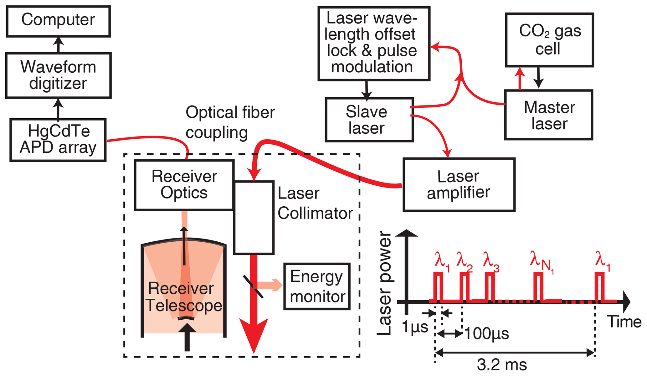
Table 1 List of laser wavelengths used in the 2017 airborne campaign for the CO₂ Sounder lidar. All wavelengths are given as the difference of the actual wavelength from the center of the 1572.335 nm CO₂ absorption line in the reference cell.

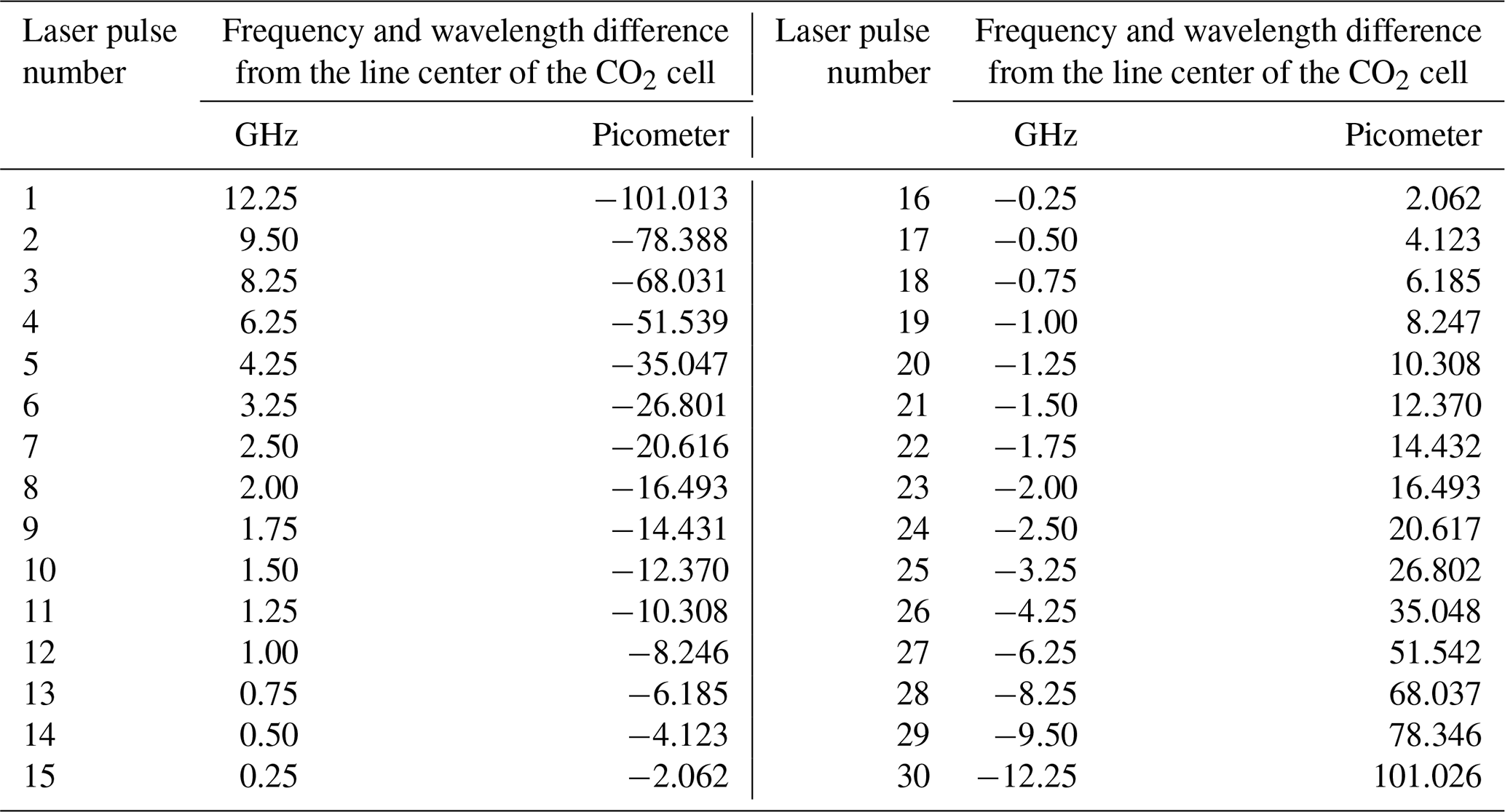
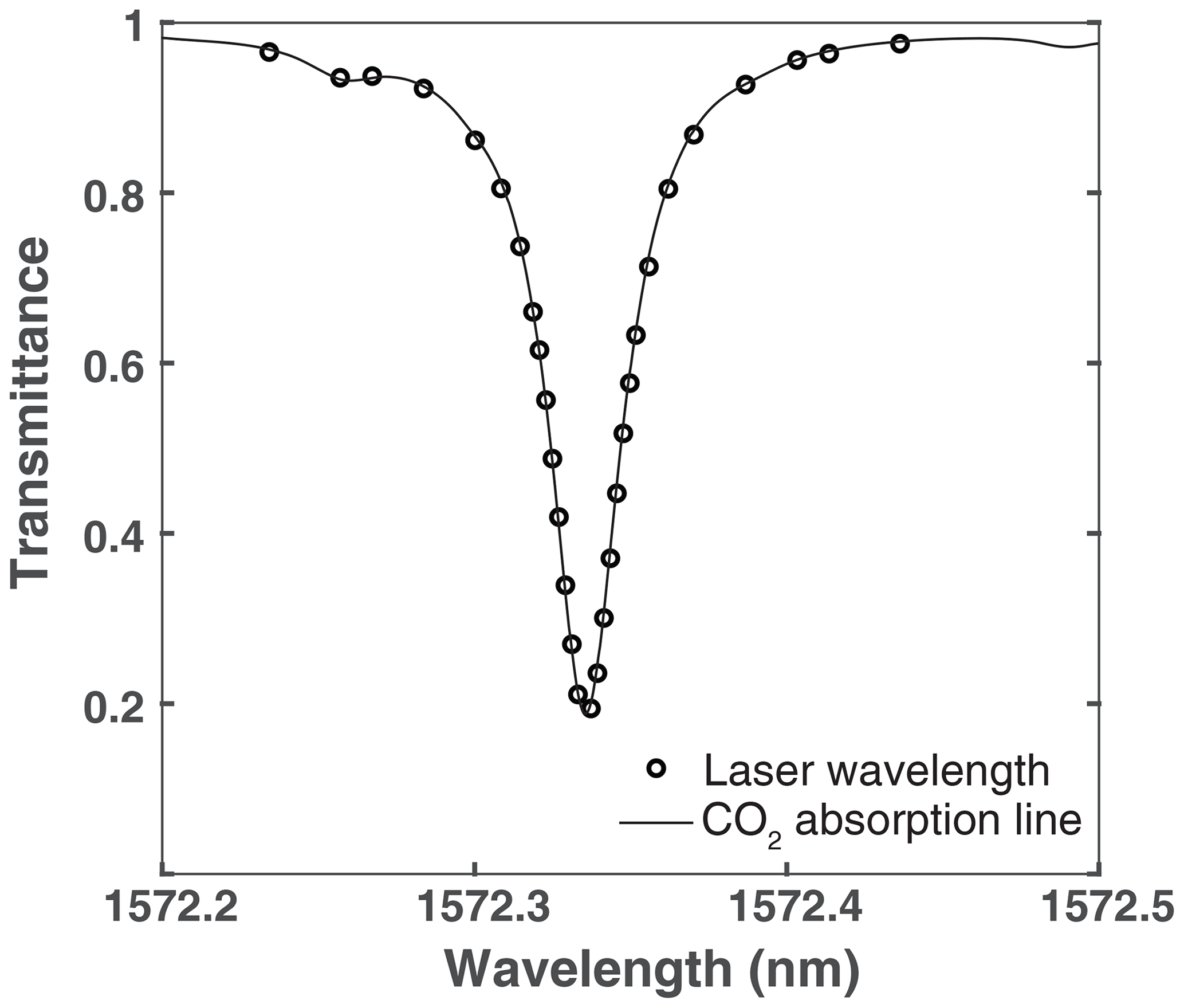
Figure 2 The laser wavelengths of the CO₂ Sounder lidar overlaid on a typical CO₂ absorption line computed for the nadir path using a modeled atmosphere.

2.2 Data structure of the airborne CO₂ Sounder lidar

The CO₂ Sounder lidar operations are synchronized with the UTC time via a GPS receiver. The measured signals are stored into data files at the end of every UTC second. The aircraft housekeeping and the GPS data are also recorded every UTC second. Each lidar data file contains nine groups of 30 received backscatter profiles, one profile for each wavelength averaged over 32 wavelength scans. Therefore, each group contains 102.4 ms of measurement data (∼ 10 Hz sample rate), and each 1 s data file contains measurement data from 32×9 wavelength scans. A DC offset of −1.1 V is added to the received waveforms before the ADC to make use of its full dynamic range (±1.25 V). At the 10 kHz pulse rate, the time between transmitted laser pulses is 100 µs. At a 100 MHz ADC sampling rate, each waveform segment contains 10 000 ADC sample points. The transmitted laser pulse waveforms are sampled and averaged by another ADC at the same sampling rate for 1000 points without adding a DC offset. The lidar controller suspends the laser wavelength scan after all the nine groups of data (a total of 921.6 ms) are collected. The remaining time before the next whole UTC second is used to generate the timestamp and combine the transmitted laser pulse waveforms into the same file. The pulse waveforms from the 31st and 32nd laser pulses during the wavelength rewind are discarded. The transmitted pulse waveforms are appended to the end of the 30th received waveform. Figure 3 shows a plot of a sample data file in the 16 bit signed integer format used by the ADCs.

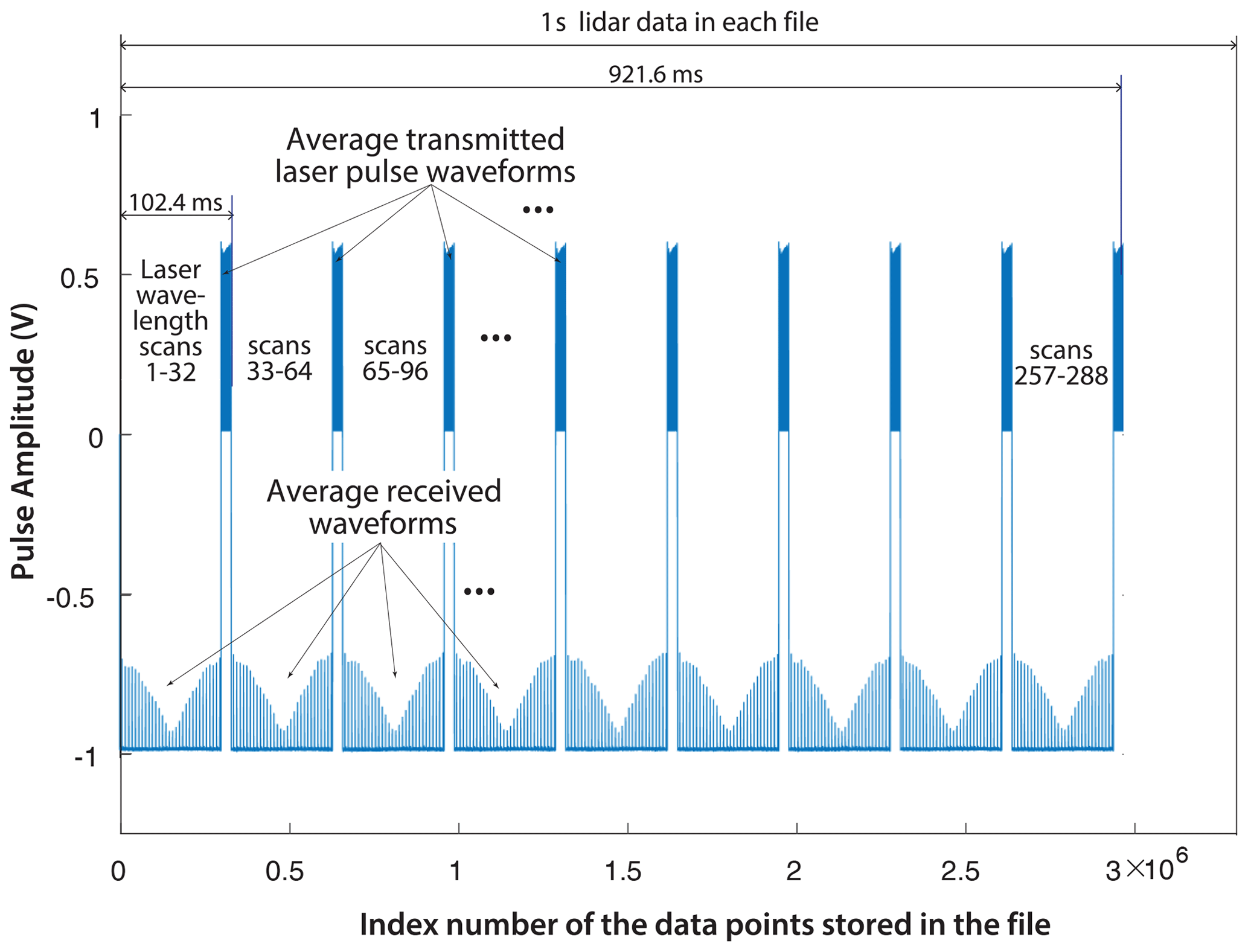
Figure 3 Plot of the recorded data file structure for the CO₂ Sounder lidar. The data were taken on 8 August 2017 at 23:30:00 (UTC) over the mountains as the aircraft flew toward the Edwards Airforce Base in California at an altitude of 11.2 km. There are nine groups of 30 pulse waveforms, one for each laser wavelength in the scan. Each is averaged over 32 scans. The corresponding waveforms for the 30 transmitted laser pulses, which are sampled at the same rate for 1000 points each, are appended to the end of the 30th received pulse waveform.

Figure 4 shows a plot of the first 30 individual pulse waveforms from the first group taken on 8 August 2017 at 23:34:00 (UTC). The first group of pulse waveforms with relatively low amplitude are from the scatter from the aircraft's nadir window. These are used as the time reference in the laser pulse time-of-flight measurements. The second group of waveforms about 50 µs after the window returns is from thin clouds, and the last set of waveforms are from the ground.

The laser is modulated with rectangular pulses but the amplitude of the actual laser pulse gradually decreases over the 1 µs pulse period. This is caused by the gradual depletion of energy stored in the fiber laser amplifier during the pulse. The detector has a slight ringing after the relatively strong ground return, which is omitted in the subsequent signal processing. There is also a small baseline offset from the detector in addition to the −1.1 V DC offset added before the ADC. The total baseline offset is estimated by averaging the waveform segment before the transmitter pulses and removed in data processing. The 30 pulse waveforms reflected by the window have nearly the same pulse amplitude. The cloud and ground return pulse waveforms show increasing variation in the detected pulse amplitude caused by atmospheric CO₂ absorption as the laser wavelengths step through the CO₂ absorption line.

Figure 4 Overlay of the 30 received pulse waveforms recorded by the airborne lidar receiver on 8 August 2017 at 23:34:00 UTC.

The XCO₂ is retrieved from the received laser pulse energies reflected by the surface. At each wavelength, the received pulse energy is calculated by first subtracting the DC offset, then integrating the pulse waveforms reflected by the ground surface and normalizing them by transmitted pulse energies. The relative atmospheric transmissions for each of the laser wavelengths are calculated as the normalized received pulse energies divided by the square of the range measured by the lidar. The surface reflectance is assumed constant during the wavelength scan. Changes in the received pulse energies at different wavelengths are attributed to the absorption by atmospheric CO₂. The XCO₂ value is retrieved via an algorithm using a linear least-squares fit of the modeled CO₂ line shape to the lidar sampled absorption line shape. Details about the signal processing for the XCO₂ retrieval can be found in Sun et al. (2021).

The signals used to calculate the atmospheric backscatter profile are contained in the same data files and are obtained by processing the signal waveforms before the ground returns. Some preliminary backscatter profiles in raw ADC units (integers) were reported earlier for this campaign (Allan et al., 2018). We have since then calibrated the backscatter profiles and released results on NASA DAAC for Biogeochemical Dynamics https://doi.org/10.3334/ORNLDAAC/2051 (Sun et al., 2022). Details of the data processing and the estimated SNR of the profiles are presented in the remainder of this paper.

3 Data processing of the atmospheric backscatter profiles from the CO₂ Sounder lidar

3.1 Level-0 data processing

The Level-0 data processing converts the raw ADC output in 16 bit integers to the atmospheric backscattered signal in the physical units of the detector output. It also removes all the known artifacts in the data, such as baseline DC offsets. To improve the SNR we averaged the backscatter profiles measured for laser wavelengths 2, 3, 4, 27, 28, 29, and 30 (seven in total). We did not include the first wavelength of the scans because occasionally the laser operation was not fully settled after the wavelength rewind. As shown in Fig. 2, these wavelengths undergo only small CO₂ absorption, so this average may be considered as a backscatter measurement at “off-line” wavelengths.

For each received pulse waveform, the DC offset from the detector is first subtracted by calculating the average detector signal for the time interval that occurs immediately before the return from aircraft window. Since the pre-window-return region is long after the ground return from the previous laser pulse but before the next one, it is composed primarily of detected solar background, the dark noise from the detector, and the DC offset of the lidar receiver. One component of the DC offset is a constant offset (−1.1 V) added to the detector output before the ADC. The other component is the inherent DC offset from the detector, which can drift slowly over time. It can also change after the detector is overloaded by excessively strong signals, such as returns from clouds in close range or returns from specular reflection at the ground.

The transmitted pulse energies are calculated from the transmitted pulse waveforms by first subtracting the DC offset and then integrating the signal over the pulse period. They are then used to normalize the corresponding received waveform. The average transmitted pulse energy over the entire flight is also recorded in the Level-0 data file. A known time delay within the lidar electrical and optical system (corresponding to a range of 26.4 m) is removed next. Following this, received pulse waveforms in the 1 s data file are averaged together to improve the SNR. Finally, the averaged pulse waveform is converted into the units of the detector output (V) by dividing the waveform data by the scale factor of the ADC.

Screening is then performed to eliminate any data with the following abnormalities: the transmitted pulse waveforms are missing in the data file, the ground return pulse is saturated with pulse amplitude above 1.1 V after removing the DC offset, or data are taken while the detector is still recovering from saturation where the estimated detector DC offset falls below 0 V or above 0.5 V after removing the known 1.1 V offset (nominal DC offset from the detector is 0.1 to 0.2 V). The mean and standard deviation of the waveform within the pre-window region for each averaged waveform is then recorded in the Level-0 data files in case further screening is needed. Lidar data that contain cloud returns within 3 km of the aircraft window are also flagged because within this distance, the laser beam does not completely overlap the receiver field of view (Allan et al., 2018). The data within this range needs to be further calibrated to account for the overlap factor.

The aircraft's navigation data are then merged with the lidar data. The aircraft flight data are obtained from archived airborne campaign housekeeping data gathered during the flight from the on-board GPS receiver and other aircraft instruments. The following parameters are extracted from the archived DC-8 housekeeping data for each second: the UTC time, latitude, longitude, altitude, pitch and roll angles, and the DC-8's radar-measured range to the surface in nadir direction.

The effect of off-nadir pointing is corrected next. The lidar is mounted to the aircraft's deck, and the laser beam is pointed down perpendicular to the deck. The aircraft flies slightly pitched up during cruise. It also performs pitch and roll maneuvers from time to time. When the laser beam is pointed away from nadir, the laser pulse travels a slant path (a longer distance) before reaching the ground. This effect, if not corrected, would result a longer length profile and a lower ground elevation when plotted with other profiles taken along nadir direction. To correct this effect, the range bin size (15 m) is first multiplied by the cosine of the combined off-nadir pointing angle. This has the effect of compressing the profile and correcting the elevation of the ground return. The resultant profile is then re-sampled by interpolating at 15 m intervals in the nadir direction. The attenuated backscatter coefficients in the corrected range bins should also be corrected for the additional attenuation by the atmosphere above the layer. Under uniform layer structure, atmospheric transmission from the aircraft to the given altitude equals $T\left({\mathit{\theta }}_{\mathrm{nadir}}\right)={\left[T\left(\mathrm{0}\right)\right]}^{\mathrm{1}/\cos \left({\mathit{\theta }}_{\mathrm{nadir}}\right)}$, with θ_nadir the laser beam pointing angle from nadir. The aircraft pitch angle was mostly within 5^∘ during cruise. The roll angle was near zero, except during sharp turns or spiral-downs. The total decrease in the two-way transmission is < 5 % under this condition. We did not correct this effect in the current data release since it is a relatively small effect for this dataset. The pitch and roll angles are included in the released data; the user may apply this correction if needed.

The surface elevation is calculated as the difference between the aircraft altitude from the on-board GPS receiver and the range measured by the lidar after correcting for the effect of off-nadir pointing angle. Missing points in the surface elevation, such as those obscured by clouds, are interpolated linearly between the elevations that border the missing region. The aircraft's latitude, longitude, altitude, pitch, and roll angle are also linearly interpolated during these conditions, if the gaps are small (seconds), and the change in measured values before and after the gap is small. All data points in the recorded waveforms above the aircraft altitude and below the ground return are removed. In the cases where there is no discernible ground return, points more than 200 m below the estimated surface elevation are removed.

Finally, the signal waveforms are vertically smoothed via a boxcar averaging window with the integration time equal to the 1 µs laser pulse width. Since the vertical resolution of the atmospheric backscatter measurements is primarily limited by the laser pulse width, the boxcar averaging has little effect on the vertical resolution of the backscatter signal, but it reduces higher frequency noise generated by the detector and the electronics.

3.2 Level-1 data processing

The Level-1 data processing converts the waveforms from the Level-0 data processing to the attenuated atmospheric backscatter profile in terms of cross section per unit volume per steradian (m⁻¹ sr⁻¹), also known as the attenuated backscatter coefficient.

The optical signal power collected by the lidar can be written as

$$\begin{array}{}\text{(1)}& y\left(t\right)=E_{\mathrm{tx}}\underset{\mathrm{0}}{\overset{{\mathit{\tau }}_{\mathrm{L}}}{\int }}x\left(\mathit{\tau }\right)h(t-\mathit{\tau })\mathrm{d}\mathit{\tau },\end{array}$$

where E_tx is the transmitted laser pulse energy in joules, x(τ) is the normalized laser pulse shape, i.e., ${\int }_{\mathrm{0}}^{{\mathit{\tau }}_{\mathrm{L}}}x\left(t\right)\mathrm{d}t\equiv \mathrm{1}$, τ_L is the laser pulse width, and h(t) is the impulse response of the atmosphere column, i.e., the normalized receiver response to an infinitely short laser pulse. Here, we assume the that lidar detector has a much faster time response than the laser pulse width, and the detector's output pulse shape is the same as that of the received optical signal.

The impulse response of the atmospheric column is related to the volume atmospheric backscatter coefficient profile by the lidar equation (Measures, 1984; Reagan et al., 1989)

$$\begin{array}{}\text{(2)}& h\left(t\right)={\displaystyle \frac{c}{\mathrm{2}}}\mathit{\beta }\left[R\left(t\right)\right]T_{\mathrm{a}}^{\mathrm{2}}\left[R\left(t\right)\right]{\displaystyle \frac{{\mathit{\eta }}_{\mathrm{r}}{A}_{\mathrm{tel}}}{R^{\mathrm{2}}\left(t\right)}}{C}_{\mathrm{1}}.\end{array}$$

Here, c is the speed of light, β[R] is the backscatter coefficient at range R in units of m⁻¹ sr⁻¹, T_a(R) is the one-way atmospheric transmission from the lidar to range R, η_r is the lidar receiver optical transmission, A_tel is the collection area of the receiver telescope, $R\left(t\right)=ct/\mathrm{2}$ is the lidar range at time t after the laser pulse emission, and C₁ is the lidar detector responsivity in V W⁻¹.

Substituting Eq. (2) into (1), the lidar signal from the detector can be written as

$$\begin{array}{}\text{(3)}& \begin{array}{rl}s\left(t\right)& =C_{\mathrm{1}}{\displaystyle \frac{c}{\mathrm{2}}}{\mathit{\eta }}_{\mathrm{r}}{A}_{\mathrm{tel}}{E}_{\mathrm{tx}}\underset{\mathrm{0}}{\overset{{\mathit{\tau }}_{\mathrm{L}}}{\int }}x\left(\mathit{\tau }\right)\\ & {\displaystyle \frac{\mathit{\beta }\left[R\left(t-\mathit{\tau }\right)\right]T_{\mathrm{a}}^{\mathrm{2}}\left[R\left(t-\mathit{\tau }\right)\right]}{R^{\mathrm{2}}\left(t-\mathit{\tau }\right)}}\mathrm{d}\mathit{\tau }.\end{array}\end{array}$$

If we assume that the atmospheric backscatter coefficient and the atmospheric transmission are approximately constant over the laser pulse interval (1 µs, or 150 m in range), the lidar signal from the detector can be written as

$$\begin{array}{}\text{(4)}& \begin{array}{rl}s\left(t\right)& \approx C_{\mathrm{1}}{\displaystyle \frac{c}{\mathrm{2}}}{\mathit{\eta }}_{\mathrm{r}}{A}_{\mathrm{tel}}{E}_{\mathrm{tx}}{\displaystyle \frac{\mathit{\beta }\left[R\left(t\right)\right]T_{\mathrm{a}}^{\mathrm{2}}\left[R\left(t\right)\right]}{R^{\mathrm{2}}\left(t\right)}}\\ & =C_{\mathrm{2}}{\displaystyle \frac{\mathrm{1}}{R^{\mathrm{2}}\left(t\right)}}\langle \mathit{\beta }\left[R\right(t\left)\right]T_{\mathrm{a}}^{\mathrm{2}}\left[R\right(t\left)\right]\rangle ,\end{array}\end{array}$$

where $C_{\mathrm{2}}=C_{\mathrm{1}}{\mathit{\eta }}_{\mathrm{r}}{A}_{\mathrm{tel}}{E}_{\mathrm{tx}}c/\mathrm{2}$ is a constant that depends only on the parameters of the lidar. Therefore, the attenuated atmospheric backscatter coefficient as a function of range can be calculated from the lidar measurement by

$$\begin{array}{}\text{(5)}& \langle \mathit{\beta }\left[R\right(t\left)\right]T_{\mathrm{a}}^{\mathrm{2}}\left[R\right(t\left)\right]\rangle =\left[R^{\mathrm{2}}\left(t\right)s\left(t\right)\right]{\displaystyle \frac{\mathrm{1}}{C_{\mathrm{2}}}}.\end{array}$$

The lidar signal term s(t) in the above equation can be expressed in terms of lidar range by substituting $t=\mathrm{2}R/c$. The attenuated backscatter coefficient can also be expressed as a function of altitude by subtracting the lidar range from the flight altitude of the aircraft.

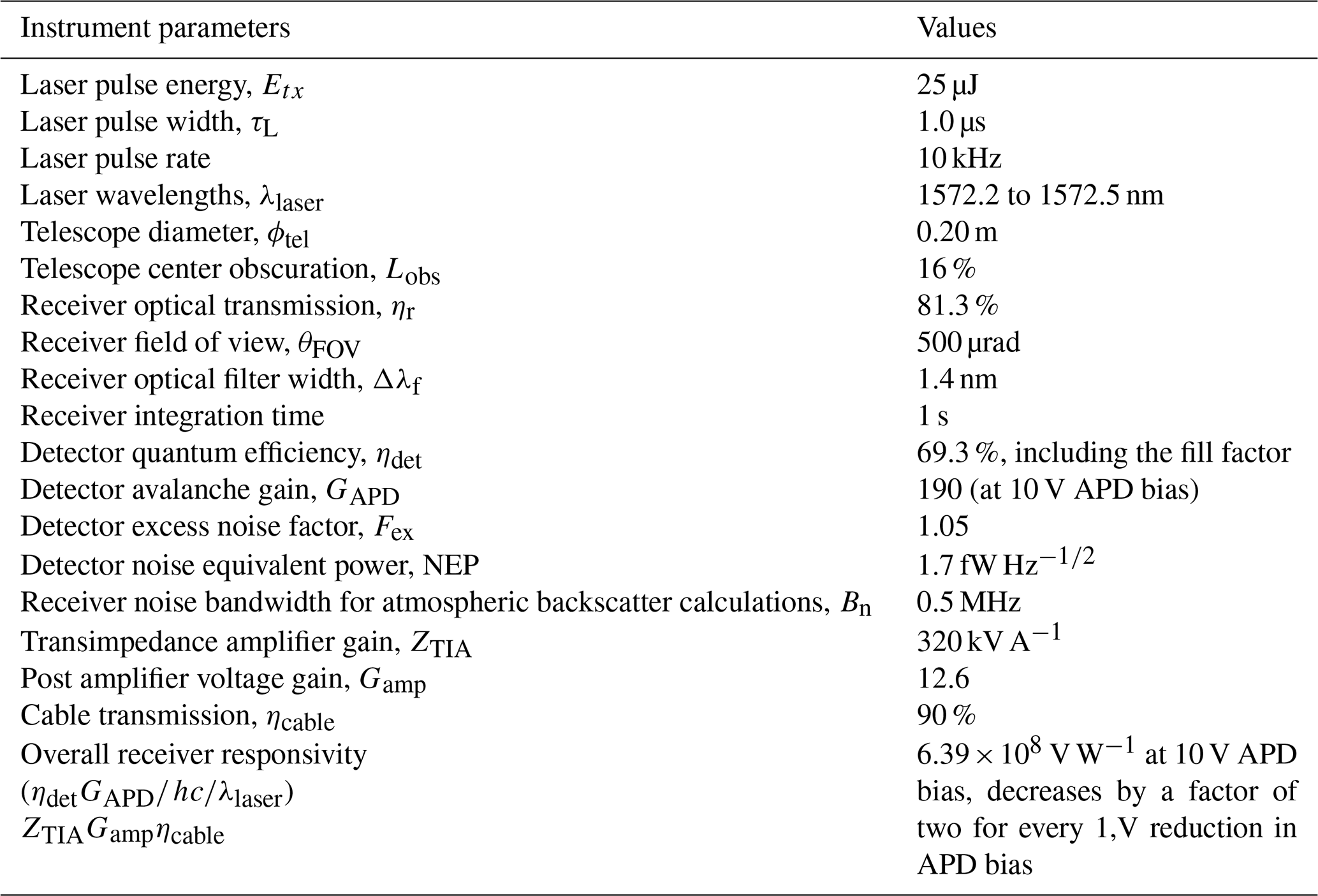
For the CO₂ Sounder lidar configuration used in the 2017 airborne campaign, the instrument constants are:

$$\begin{array}{}\text{(6)}& {\displaystyle }{C}_{\mathrm{1}}& {\displaystyle }=\left({\mathit{\eta }}_{\det }{G}_{\mathrm{APD}}{\displaystyle \frac{\mathrm{1}}{E_{\mathrm{ph}}}}{e}_{\mathrm{c}}\right)Z_{\mathrm{TIA}}{G}_{\mathrm{amp}}{\mathit{\eta }}_{\mathrm{cable}},\left(\mathrm{V}{\mathrm{W}}^{-\mathrm{1}}\right),\text{(7)}& {\displaystyle }{C}_{\mathrm{2}}& {\displaystyle }=C_{\mathrm{1}}{\mathit{\eta }}_{\mathrm{r}}{A}_{\mathrm{tel}}{E}_{tx}{\displaystyle \frac{c}{\mathrm{2}}}=C_{\mathrm{1}}{\mathit{\eta }}_{\mathrm{r}}{\displaystyle \frac{\mathit{\pi }{\mathit{\varphi }}_{\mathrm{tel}}^{\mathrm{2}}}{\mathrm{4}}}\left(\mathrm{1}-L_{\mathrm{obs}}\right)E_{tx}{\displaystyle \frac{c}{\mathrm{2}}}.\left(\mathrm{V}{\mathrm{m}}^{\mathrm{3}}\right).\end{array}$$

Here, η_det is the detector quantum efficiency, G_APD is the APD gain, $E_{\mathrm{ph}}=hc/{\mathit{\lambda }}_{\mathrm{laser}}$ is the laser photon energy, h is Planck's constant, λ_laser is the laser wavelength, e_c is the electron charge, Z_TIA is the gain of the preamplifier (a transimpedance amplifier) in V W⁻¹, G_amp is the post amplifier voltage gain, η_cable is the electrical cable transmission, ϕ_tel is the receiver telescope diameter, and L_obs is the fractional loss of the telescope's collection area caused by its center obscuration.

Table 2 lists the values of these parameters for the 2017 CO₂ Sounder lidar. The resultant detector responsivity is $C_{\mathrm{1}}=\mathrm{6.39}\times {\mathrm{10}}^{\mathrm{8}}$ V W⁻¹ for nominal APD gain, and the instrument constant is $C_{\mathrm{2}}=\mathrm{5.13}\times {\mathrm{10}}^{\mathrm{10}}$ V m³.

Table 2 CO₂ Sounder Lidar parameters as used in the 2017 airborne campaign.

The received signal level from the surface varies with lidar range. To prevent detector saturation, the gain of the lidar detector was adjusted manually during the flight to keep the received signal within the detector linear dynamic range. The detector gain was changed in steps of 2 by adjusting the bias voltage of the HgCdTe APD detector. In the data processing, the detector's gain value was determined from the pulse amplitude of the window returns. After filtering out anomalous window returns, which generally resulted from the aircraft flying through clouds, the pulse energies and the centroid of the window returns are calculated and binned for each 1 s data file for each flight. The window return pulse energies are divided into groups separated by a factor of 2. The average value from the bins with the APD biased at 10 V is defined as the nominal. Measurements made with window return pulse amplitude equal to $\mathrm{1}/\mathrm{2}$ the nominal are assigned to have a gain correction factor of 2, and their backscatter waveforms are multiplied by 2. For those with window return pulse amplitudes equal to $\mathrm{1}/\mathrm{4}$ their backscatter waveforms are multiplied by a factor of 4, etc. When the window return pulse energy is an outlier or too weak to determine, the last known valid detector gain value is used.

For each second, the attenuated atmosphere backscatter coefficient is obtained by multiplying the signal waveforms from Level-1 data processing by the square of the lidar range and then dividing it by the lidar scaling factor C₂ according to Eq. (5). Figure 5 shows the atmosphere backscatter profile for the flight on 8 August 2017 along the flight path shown in Fig. 6. Figures 7 and 8 show expanded views of the same data. During this flight, aircraft flew over mountains, ocean, desert, etc. (Fig. 6) and performed seven spiral-down maneuvers to compare the lidar XCO₂ measurements with those from the in situ gas analyzer on board the aircraft. The surface type and reflectance affected the solar background noise in the atmospheric backscatter measurement. For example, when the aircraft flew over ocean surface in between Spiral-Downs #3 and #4, the scattered sunlight was much lower than that for land surfaces, and the noise in the received data became noticeably lower, as shown in Fig. 5. Figure 9 shows a line plot of the vertical atmospheric backscatter profile measured at time 23:34:00 UTC.

The raw lidar signal is digitized at 10 ns (1.5 m) intervals by the ADC to enable meter-level calculations of the lidar range to the surface. However, the vertical resolution of the computed atmospheric backscatter profiles is much wider due to the 1 µs (150 m) laser pulse width. To reduce the data volume, the backscatter profile data are re-sampled with 100 ns (15 m) bin width. This still oversamples the backscatter profile but preserves certain temporal features in the data, such as the ground returns and cloud boundaries. The horizontal resolution along the aircraft ground track is the distance traveled by the aircraft in 1 s, or about 200 m. These results from most flights showed the values of attenuated backscatter coefficients within the boundary layer are comparable to those reported by Spinhirne et al. (1997), which were measured at a nearby (1540 nm) laser wavelength. Similar atmospheric backscatter profiles have been measured with a ground-based 2 µm lidar that used the same type of HgCdTe APD detector (Refaat et al., 2020).

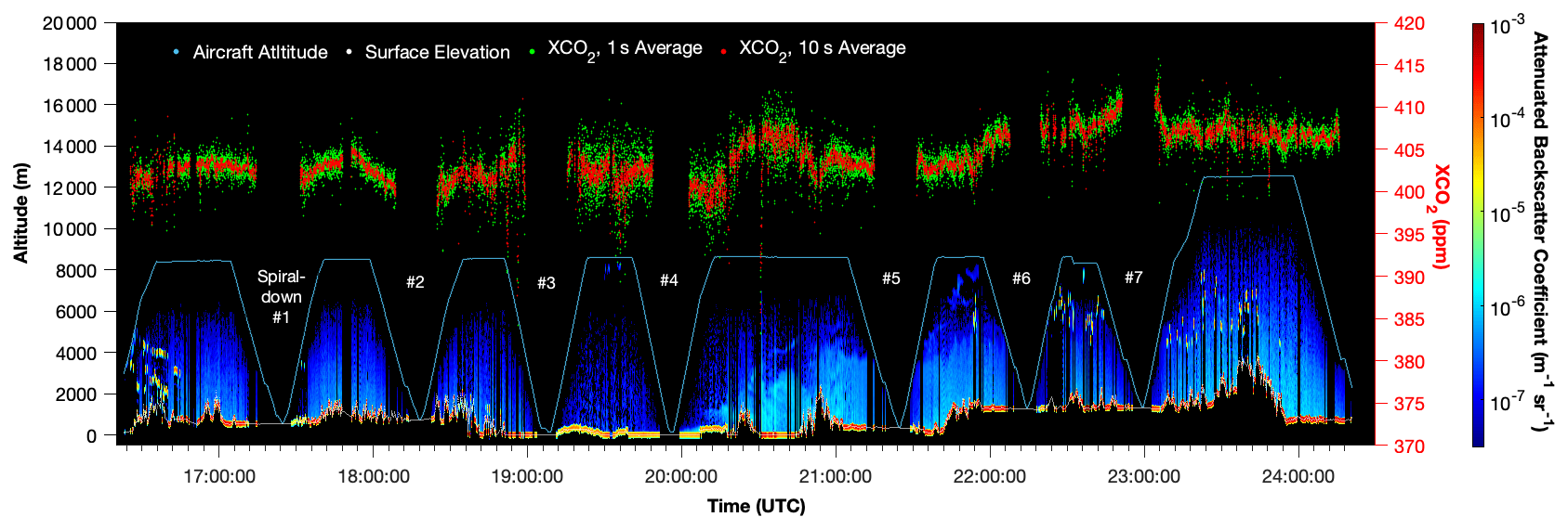
Figure 5 Time history of the attenuated atmospheric backscatter profiles measured by the CO₂ Sounder lidar during the flight on 8 August 2017 along with the retrieved values of XCO₂.

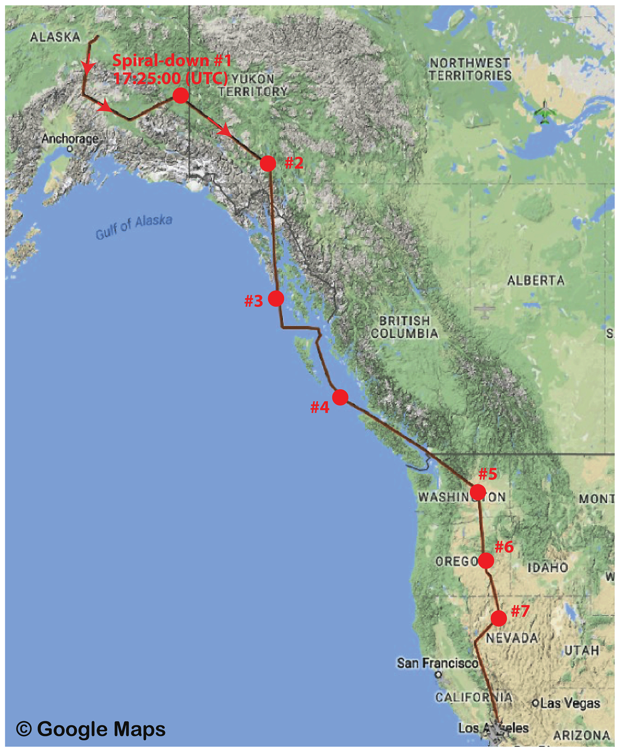
Figure 6 The flight path of the airborne CO₂ Sounder lidar on 8 August 2017 (plotted via Google Maps). Each dot indicates a spiral-down maneuver.

Figure 7 Same as Fig. 5 but expanded for the last segment from time 23:00:00 UTC to the end of the flight.

Figure 8 Same as Fig. 7 but expanded for the 5 min between 23:30:00 and 23:35:00 UTC.

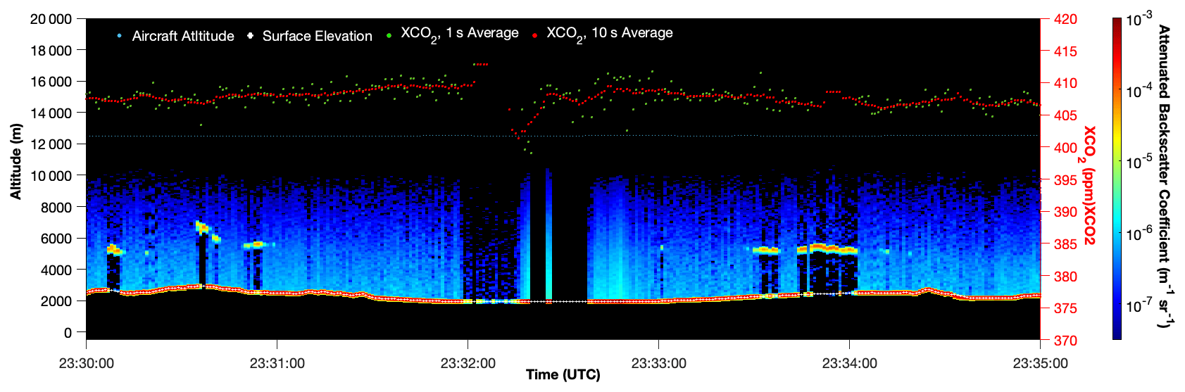
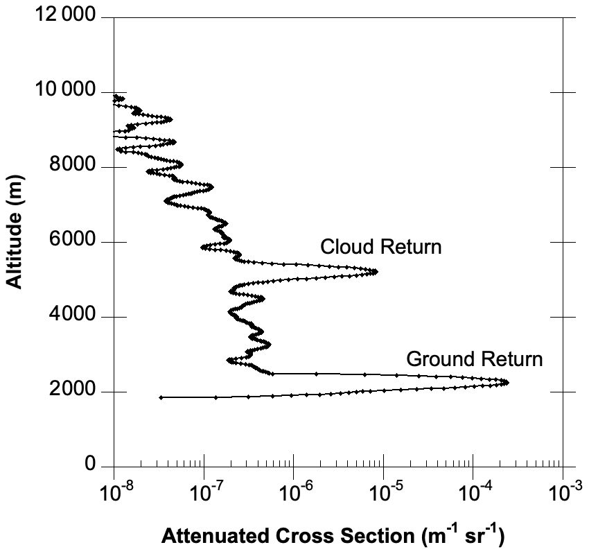
Figure 9 Plot of the attenuated backscatter profile and ground return measured on 8 August 2017 at 23:34:00 UTC with a 15 m vertical sampling interval. The results are from the same data shown in Fig. 4 after Level 1 processing.

These backscatter profiles also contain the broadened lidar returns from the ground expressed in terms of attenuated backscatter coefficient. With the 1.0 µs wide laser pulse and the 1.0 µs wide boxcar smoothing, the smoothed return signal is usually triangular with a width of 10 range bins at the half maximum points and 20 range bins at the base. Any changes in surface elevation during the receiver integration time can cause additional broadening of the return pulse shape to 15 to 20 range bins (1.5 to 2 µs), as shown in Fig. 9. These ground return signals at the end of the backscatter profiles can be used to calculate the attenuated surface reflectance by summing the backscatter values over all the range bins containing the ground return and then multiplying the results by π and the bin width (15 m). Figure 10 shows the attenuated surface reflectance as the aircraft approached the Edward Air Force Base on 8 August 2017. Over a mountainous area for the time period from 23:00:00 to 23:40:00 UTC, the attenuated surface reflectance varied between about 4 % when there were clouds and 18 % when it was cloud free. The average attenuated surface reflectance from 00:01:00 to 00:11:00 UTC over desert near the end of the flight was 22 %. If we estimate the average desert reflectance to be 45 % (Kuze et al., 2011), the one-way atmospheric transmission would be 70 %, which is consistent with the sky condition shown on the aerial photograph (Fig. 11). When the surface reflectance can be estimated by some other means, the lidar profiles may be used to calculate the extinction to backscatter ratio of thin clouds and aerosols in the path.

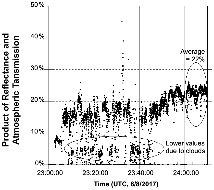
Figure 10 Product of the surface reflectance and two-way atmospheric transmission calculated by integrating the ground return of the backscatter profile as the aircraft flew toward the Edwards Air Force Base during 8 August 2017.

Figure 11 Photograph taken from the aircraft to the Edwards Air Force Base on 8 August 2017 24:14:00 UTC showing the sky condition for the last segment of data shown in Fig. 10.

4 Signal to noise ratio calculations

To derive the SNR of the attenuated backscatter profiles we first express the average detected signal from each laser pulse given by Eq. (4) in terms of the rate of detected signal photons as a function of the lidar range, as

$$\begin{array}{}\text{(8)}& \langle {\dot{n}}_{\mathrm{sig}}\left(R\right)\rangle \approx {\displaystyle \frac{c}{\mathrm{2}}}{\displaystyle \frac{E_{\mathrm{tx}}}{E_{\mathrm{ph}}}}{A}_{\mathrm{tel}}{\mathit{\eta }}_{\det }{\mathit{\eta }}_{\mathrm{r}}{\displaystyle \frac{\langle T_{\mathrm{a}}^{\mathrm{2}}\left(R\right)\rangle \langle \mathit{\beta }\left(R\right)\rangle }{R^{\mathrm{2}}}},\end{array}$$

where R is the lidar range.

For each laser pulse, the standard deviation of the rate of the detected signal photons can be calculated as (Gagliardi and Karp, 1995)

$$\begin{array}{}\text{(9)}& \begin{array}{rl}& {\mathit{\sigma }}_{\mathrm{noise}}\left(R\right)=\\ & \sqrt{\left\{F_{\mathrm{ex}}\left[\langle {\dot{n}}_{\mathrm{sig}}\left(R\right)\rangle +\langle {\dot{n}}_{\mathrm{b}}\rangle \right]+{\left(\mathrm{NEP}{\displaystyle \frac{{\mathit{\lambda }}_{\mathrm{laser}}}{hc}}\right)}^{\mathrm{2}}\right\}{B}_{\mathrm{n}}},\end{array}\end{array}$$

where F_ex is the detector excess noise factor from the randomness of the APD gain, $\langle {\dot{n}}_{\mathrm{b}}\rangle$ is the average detected background photon rate, NEP is the detector noise equivalent power due to the detector dark noise and the preamplifier noise, and B_n is the noise bandwidth of the lidar receiver used for the atmospheric backscatter calculations. The noise bandwidth is equal to $\mathrm{1}/\mathrm{2}{t}_{\mathrm{box}}$ with t_box the width of the boxcar averaging window in the signal processing.

For the CO₂ Sounder lidar, the lidar range R in Eqs. (9) and (10) consists of a discrete set of lidar ranges for a series of range bins. Although the attenuated atmospheric backscatter profiles are given in the 15 m range bin size, the actual profiles are averaged over 150 m vertical layers due to the effect of the laser pulse width and the boxcar smoothing in the data processing. Therefore, the noise standard deviation given in Eq. (10) is for the 150 m vertical integration interval. This noise may be further reduced by averaging data from adjacent 150 m vertical atmospheric layers.

When the lidar views a sunlit diffuse scattering surface through a clear sky the average detected background photon rate is given by

$$\begin{array}{}\text{(10)}& \langle {\dot{n}}_{\mathrm{b}}\rangle =I_{\mathrm{s}}\mathrm{\Delta }{\mathit{\lambda }}_{\mathrm{f}}\mathit{\pi }{\left({\displaystyle \frac{{\mathit{\theta }}_{\mathrm{FOV}}}{\mathrm{2}}}\right)}^{\mathrm{2}}{\displaystyle \frac{\mathit{\rho }}{\mathit{\pi }}}\cdot A_{\mathrm{tel}}{\mathit{\eta }}_{\mathrm{r}}{\mathit{\eta }}_{\det },\end{array}$$

where I_s is the solar irradiance at the 1572 nm laser wavelength, Δλ_f is the receiver optical filter bandwidth, θ_FOV is the receiver field of view diameter, and ρ is the diffuse reflectance of the surface. These and other instrument parameter values are listed in Table 2.

For a single laser pulse, the SNR of the attenuated backscatter coefficient measurement is the same as the SNR of the rate of detected signal photons, which is the ratio of Eqs. (9) to (10). Therefore, the SNR of a 150 m vertical bin at range R when averaged over the number of laser pulse measurements within the 1 s receiver integration time is given by

$$\begin{array}{}\text{(11)}& {\mathrm{SNR}}_{\mathrm{av}}\left(R\right)=\sqrt{N_{\mathrm{ave}}}{\displaystyle \frac{\langle {\dot{n}}_{\mathrm{sig}}\left(R\right)\rangle }{{\mathit{\sigma }}_{\mathrm{noise}}\left(R\right)}},\end{array}$$

with N_ave the total number of laser pulses measured within the receiver integration time. For the CO₂ Sounder lidar with a 1 s receiver integration time, $N_{\mathrm{ave}}=\mathrm{32}\times \mathrm{9}\times \mathrm{7}=\mathrm{2016}$.

The SNR is proportional to the attenuated backscatter coefficient and inversely proportional to the square of the lidar range. Hence, for measurements from an airborne lidar, the SNR is a strong function of the range to the atmospheric layers being measured. Figure 12 shows the calculated SNR of the attenuated backscatter coefficient vs. the lidar range for 10⁻⁶, 10⁻⁵, and 10⁻⁴ m⁻¹ sr⁻¹ backscatter coefficients at local noon and night. For example, for a 12 km aircraft altitude above ground surface and a 1 s receiver integration time, the averaged SNR is about 65 for clouds with a backscatter coefficient of 10⁻⁵ m⁻¹ sr⁻¹ that are 7 km below the aircraft (5 km above surface) during daytime at 45^∘ sun angle. Therefore, these attenuated backscatter profiles can be used to reliably identify mid-altitude clouds. The signals from aerosols at lower altitudes are much weaker. For example, at 10 km lidar range in the daytime, the averaged SNR for a 1 s integration time is about 2.0 for aerosols with a backscatter coefficient of 10⁻⁶ m⁻¹ sr⁻¹.

As a comparison, we calculated the average attenuated backscatter coefficient profile and the corresponding SNR from 100 consecutive backscattering profiles starting from 8 August 2017, at 23:55:00 UTC (a small cloud-free segment shown in Fig. 7). The mean and the ratio of the mean to standard deviation are plotted in Fig. 13. The ratio of the mean to standard deviation gives an estimate of the SNR. It is about 2.4 for attenuated backscattering coefficients of 10⁻⁶ m⁻¹ sr⁻¹ at 4.8 km altitude (7.8 km lidar range). The extrapolated SNR at 10 km lidar range is 1.5. The SNR estimated from the measurement data is expected to be lower since it also includes the effects of small atmosphere variation during the measurement period. The SNR can be improved by averaging over more measurements along the flight path and thicker vertical layer.

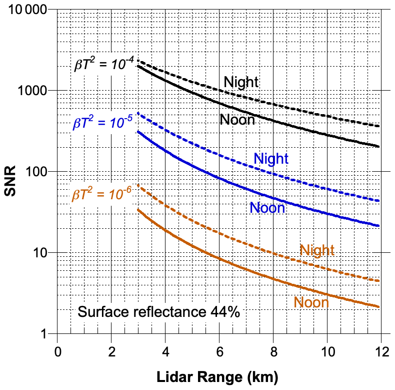
Figure 12 Estimated SNR of the attenuated backscatter coefficients obtained from the CO₂ Sounder lidar in the 2017 airborne campaign for 1 s integration times and 150 m vertical resolution. The SNR of the backscatter profiles may be further improved by averaging over a longer time intervals and by using thicker atmospheric layers.

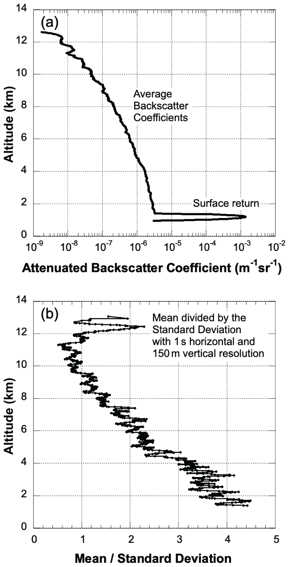
Figure 13 Average attenuated backscatter coefficients and the ratio of the mean to standard deviation calculated from 100 consecutive backscattering profiles starting on 8 August 2017 at 23:55:00 UTC.

5 Data availability

The atmospheric backscatter profiles by the CO₂ Sounder from the 2017 airborne lidar measurements are available from the NASA Oak Ridge National Laboratory (ORNL) Distributed Active Archive Center (DAAC) for Biogeochemical Dynamics, https://doi.org/10.3334/ORNLDAAC/2051 (Sun et al., 2022). NASA Earth Science Data are published under an arrangement equivalent to a CC0 license. All data are openly shared, without restriction, in accordance with the EOSDIS Data Use Policy posted at https://earthdata.nasa.gov/earth-observation-data/data-use-policy?_ga=2.94803679.255626558.1646145252-1577112238.1614541217 (last access: 19 August 2022).

6 Code availability

The software codes used for the data processing of the atmospheric backscatter profiles described in this paper are posted on the same data depository website as the data, https://doi.org/10.3334/ORNLDAAC/2051 (Sun et al., 5 2022).

7 Conclusions

In addition to measuring the column average CO₂ mixing ratio (XCO₂), the NASA GSFC CO₂ Sounder lidar measures the attenuated atmospheric backscatter profiles in the laser beam's path. We have recently processed the atmospheric backscatter profiles from the 2017 ASCENDS/ABoVE (Active Sensing of CO₂ Emission over Nights, Days, and Seasons /Arctic Boreal Vulnerability Experiment) airborne campaign and produced a new dataset of range-resolved attenuated atmospheric backscatter coefficients at 1572 nm laser wavelength measured for each of the eight flights. The analysis shows that the signal to noise ratios of the CO₂ Sounder lidar backscatter profiles are sufficient to identify clouds and estimate the height of aerosol layers. This new dataset also provides additional information to help interpret the retrieved XCO₂. These same types of measurements may be obtained in the future from a space-based lidar that uses the same measurement technique and scaled for a similar power-aperture product.

Appendix A

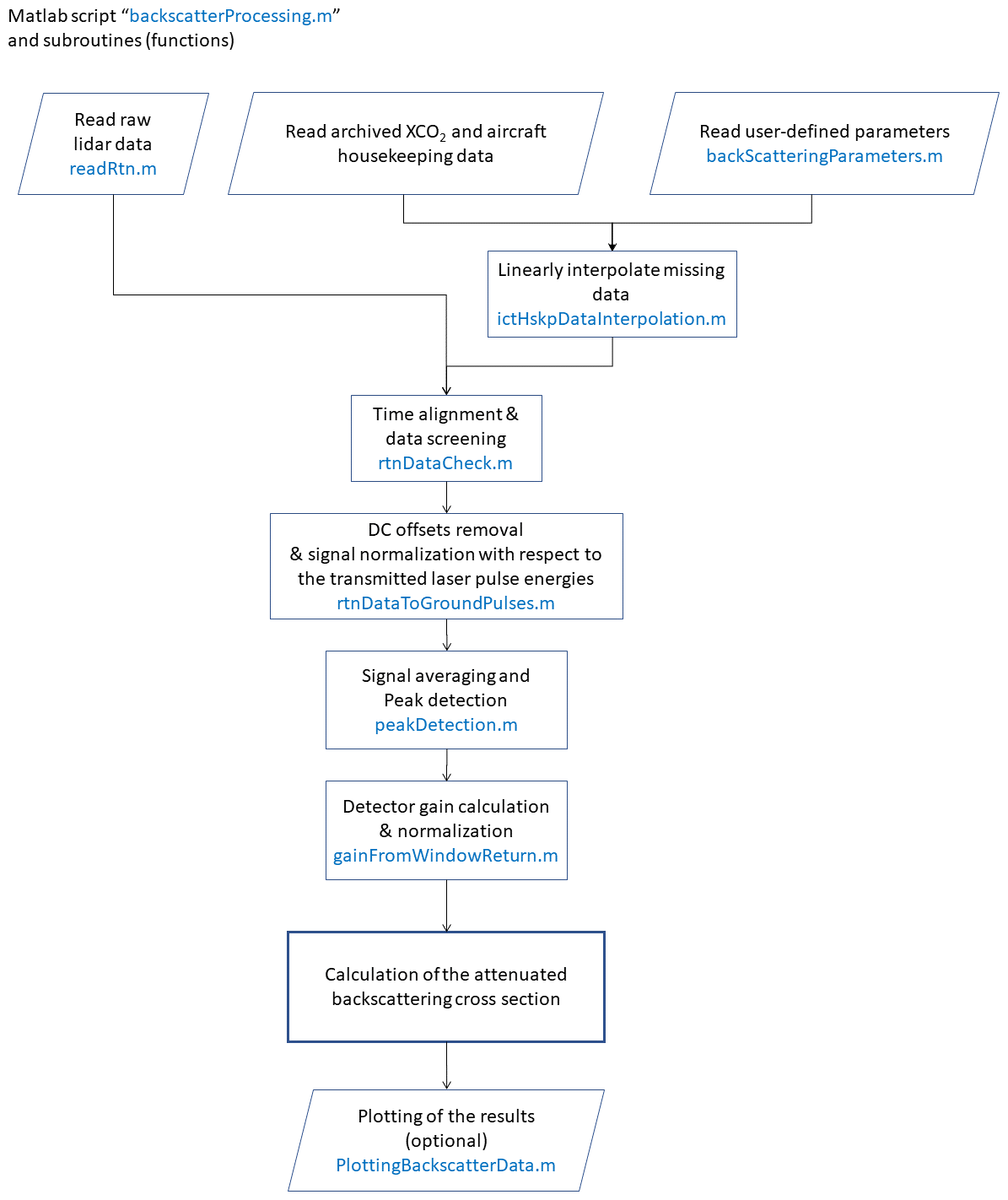
The following is the flowchart of the data processing software, which was developed using Matlab. The software consists of a main program “backscatterProcessing.m” and a set of functions indicated in blue text. The software code is available at the same website, where the atmospheric backscatter profiles are archived (https://doi.org/10.3334/ORNLDAAC/2051, Sun et al., 2022).

Figure A1 Flowchart of the software used to process the data described in this paper.