the Creative Commons Attribution 4.0 License.
the Creative Commons Attribution 4.0 License.
 | 26 Aug 2022
Combined high-resolution rainfall and wind data collected for 3 months on a wind farm 110 km southeast of Paris (France)
Jerry Jose
Ioulia Tchiguirinskaia
Daniel Schertzer
The Hydrology Meteorology and Complexity laboratory of École des Ponts ParisTech (http://hmco.enpc.fr, last access: 16 August 2022) has made a data set of high-resolution atmospheric measurements available, which is of interest for the atmospheric science community. It comes from a campaign carried out in the framework of the Rainfall Wind Turbine or Turbulence project (RW-Turb; supported by the French National Research Agency, grant no. ANR-19-CE05-0022) on a meteorological mast installed at a wind farm located approx. 110 km southeast of Paris in France. In total, 3 months of data, covering the spring period from 1 March to 1 June 2021, are made available. We used six devices, namely two 3D sonic anemometers (manufactured by Thies), two mini meteorological stations (manufactured by Thies), and two disdrometers (Parsivel2, manufactured by OTT). They are installed at two heights (approx. 45 and 80 m), which enables us to monitor potential effects of altitude. The temporal resolution is of 100 Hz for the 3D sonic anemometers, 1 Hz for the meteorological stations, and 30 s for the disdrometers. A multifractal analysis is implemented to assess the effective resolution of the devices, and it is suggested that the anemometers and stations are able to measure expected variability only down to 1 and 16 s, respectively. A link to the data set can be found at https://doi.org/10.5281/zenodo.5801900 (Gires et al., 2021)
- Article
(4769 KB) - Full-text XML
- BibTeX
- EndNote


A limited number of studies have investigated the effect of rainfall on wind turbines, and they tend to indicate that it is rather significant. For example, Corrigan and Demiglio (1985) reported a power production decrease of 20 % to 30 % from an experiment conducted in Ohio (USA) on a 38 m diameter two-blade wind turbine, with a greater worsening with greater rain rates. Walker and Wade (1986) slightly disputed those results for light rain (i.e. a rain rate less than 8 mm h−1). In fact, on the contrary, they found an increase of a few percent for light rain and attributed it to modifications of blade roughness or wind measurement issues. The significant decrease was later confirmed experimentally (Al et al., 2011) and with multiphase (volatile for air and liquid for rain) computational fluid dynamics (Cai et al., 2013; Cohan and Arastoopour, 2016).
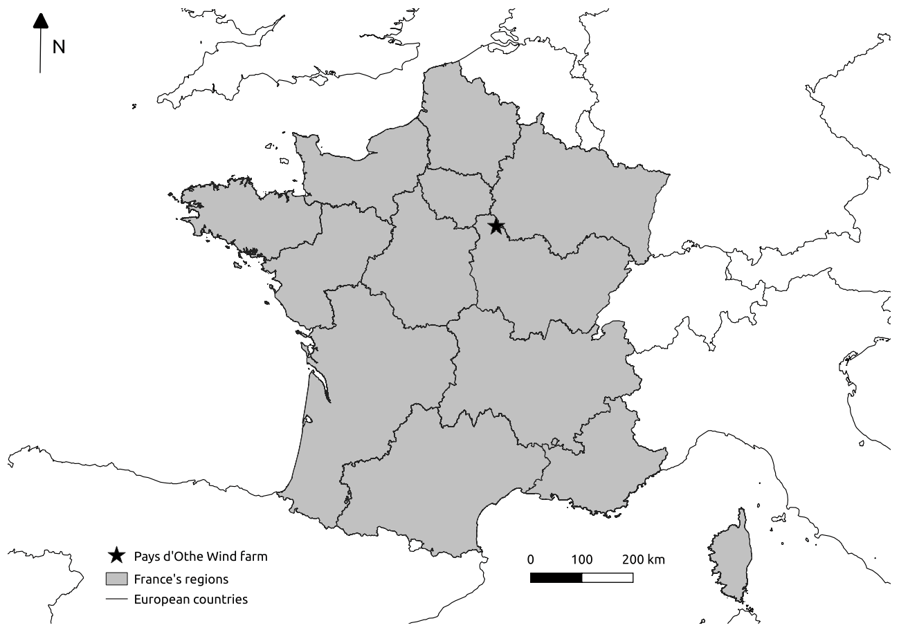
Figure 1Location of the Pays d'Othe wind farm in France, where the data presented in this paper are collected from.
Understanding the effect of rainfall on wind power production is hence highly relevant. The Rainfall Wind Turbine or Turbulence project (RW-Turb), which is supported by the French National Research Agency (ANR in French), actually aims at contributing to the topic. The data presented in the paper were collected in the framework of this project. In order to properly address the topic, two distinct aspects should be studied properly; first, the rainfall effect on the energy resources, and second, the rainfall effect on the conversion process of wind power to electric power by the wind turbine. To this end, rainfall should not only be understood, as commonly done, as a simple rain rate expressed in millimetres per hour (mm h−1) but also by considering its full complexity through the spatial and temporal variability in the drop size distribution (DSD). The data set shared is especially tailored for this point. Indeed, both the wind energy and torque available to wind turbines are basically proportional to the power of the instantaneous wind speed. As wind is neither constant nor uniform, taking into account its small-scale spatiotemporal fluctuations is crucial to properly quantify the integrals of these quantities, especially given that the wind turbines are located in the atmospheric boundary layer, which is an area of increased complexity due to the interactions with the ground. Improving turbulence understanding has been listed among the scientific challenges of this field in a recent joint paper by leading academics of the field (van Kuik et al., 2016, for the European Academy of Wind Energy, EAWE). The intrinsically intermittent nature of wind, i.e. the fact that its activity becomes located on smaller and smaller support as the observation scale decreases, makes it complex to analyse, notably requiring appropriate theoretical framework and high-resolution measuring devices. An illustration of this can be found in Fitton et al. (2011, 2014), in which authors studied 3D wind data collected from two different locations (Corsica and Germany) in a multifractal framework, enabling them to highlight the need to investigate turbulence in a 3D framework so that the anisotropy between the horizontal and vertical wind components is accounted for. They also pointed out that such a scale invariant framework is needed to explain the power law fall-off for the probability distribution of wind fluctuations and to account for the observed sporadic bursts, which are not treated in a standard Gaussian framework that strongly underestimates the extremes. Rainfall was not considered in such an analysis up to now.
Hence, given the numerous potential applications of combined high-resolution rainfall and wind data, notably in the framework of wind energy production, the Hydrology Meteorology and Complexity laboratory of École des Ponts ParisTech (HM&Co-ENPC) considers that it is relevant to make the data available to the scientific community from a 3-month (1 March–1 June 2021) measurement campaign carried out on a meteorological mast operated by Boralex, a wind power producer. The campaign involves six devices, namely a 3D sonic anemometer, a disdrometer (which gives access to the size and velocity of drops falling through its sampling area), and a mini meteorological station located at roughly 78 m; the same setting is repeated at roughly 45 m. The devices' functioning and the measurement campaign is presented in Sect. 2. The corresponding database and available tools are presented in Sect. 3.
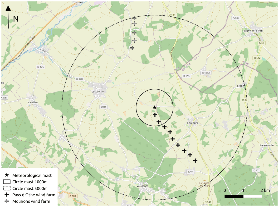
Figure 2Map of the surroundings of the meteorological mast used. The background of the map is taken from OpenStreetMap (https://www.openstreetmap.org/, last access: 16 August 2022, © OpenStreetMap contributors 2021. Distributed under the Open Data Commons Open Database License (ODbL) v1.0.). Forests are in green, farms are in light green, residential areas are in grey, and roads are in white (small ones) or orange (highways).
Before proceeding further, the purpose of the paper should be clarified to avoid any misunderstanding. It is a data paper that aims at presenting, in detail, a data set made available to the community. It does not aim at fully exploiting the data set for scientific studies; this will be done in further dedicated papers by the authors or community members using it. The data set was collected in a framework designed for application in wind energy, but potential applications of such a high-resolution rainfall and wind measurement campaign are much wider. For example, understanding rainfall processes remains a major challenge in the field of hydrology. The lack of a precise space–time distributed measurement is one of the greatest sources of uncertainty in hydrological modelling. Improving our understanding of rainfall requires an in-depth understanding of its relationship to wind turbulence across scales. This could notably lead to the development of a 3D+1 model for the drops' location, which could be used to overcome the simplistic assumption of homogeneous distribution within a radar gate (see Gires et al., 2016, and references therein for an initial discussion on the topic) or to improve wind drift correction scheme for radar algorithms. Such developments will improve precipitation estimation with the help of radars.
2.1 Location of the meteorological mast
The devices involved in this measurement campaign are installed on a meteorological mast located on a wind farm at Pays d'Othe, France. This wind farm is made of nine wind turbines and is jointly operated by Boralex (https://www.boralex.com/our-projects-and-sites/, last access: last access: 16 August 2022) and JP Énergie Environnement (https://pays-othe-89.parc-eolien-jpee.fr/, last access: last access: 16 August 2022). It is located at roughly 110 km southeast of Paris, on the territory of the cities of Vaudeurs, Coulours, and Les Sièges (see Fig. 1). Figure 2 displays a magnified map of the surroundings, with an OpenStreetMap background. The meteorological mast is the star in the middle. The nine wind turbines of the Pays d'Othe wind farm are aligned southeast of it and within a 4 km radius (black vertical crosses). They are visible in the left and right panels of Fig. 3. The five turbines of the Molinons wind farm in the north are also visible within the 5 km radius (grey vertical crosses). It should also be noted that a small grove is located just south of the mast at roughly 160 m. A larger one is in the East at roughly 100 m. These groves are also visible on the middle panel of Fig. 3.
Figure 4 displays the elevation around the meteorological mast. The data used are the IGN DBALTI 75M. The data have a horizontal resolution of 75 m and are provided by the National Institute of Geographic and Forest Information (IGN). The elevation of the pixel where the mast is located is 230 m. Nearby the mast (i.e. within a 1 km radius), there is a small slope in the north–south direction, which is visible in the right panel of Fig. 3.
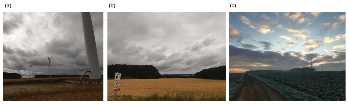
Figure 3Pictures of the Pays d'Othe wind farm. (a) Picture of the wind farm taken from the wind turbine closest to the mast. (b) Picture of the meteorological mast taken from the wind turbine closest to it. (c) Picture of the mast (left of the picture) and the wind farm (right of the picture) taken from the road just north of the mast. Pictures were taken by Auguste Gires.
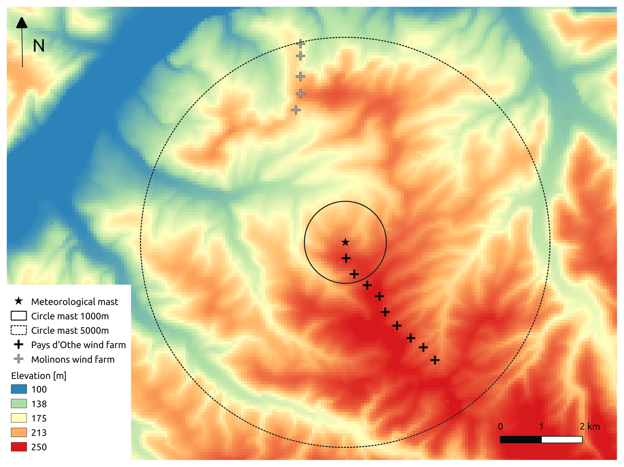
Figure 4Elevation map around the Pay d'Othe wind farm. For the elevation in metres, the IGN DBALTI 75M product is used.
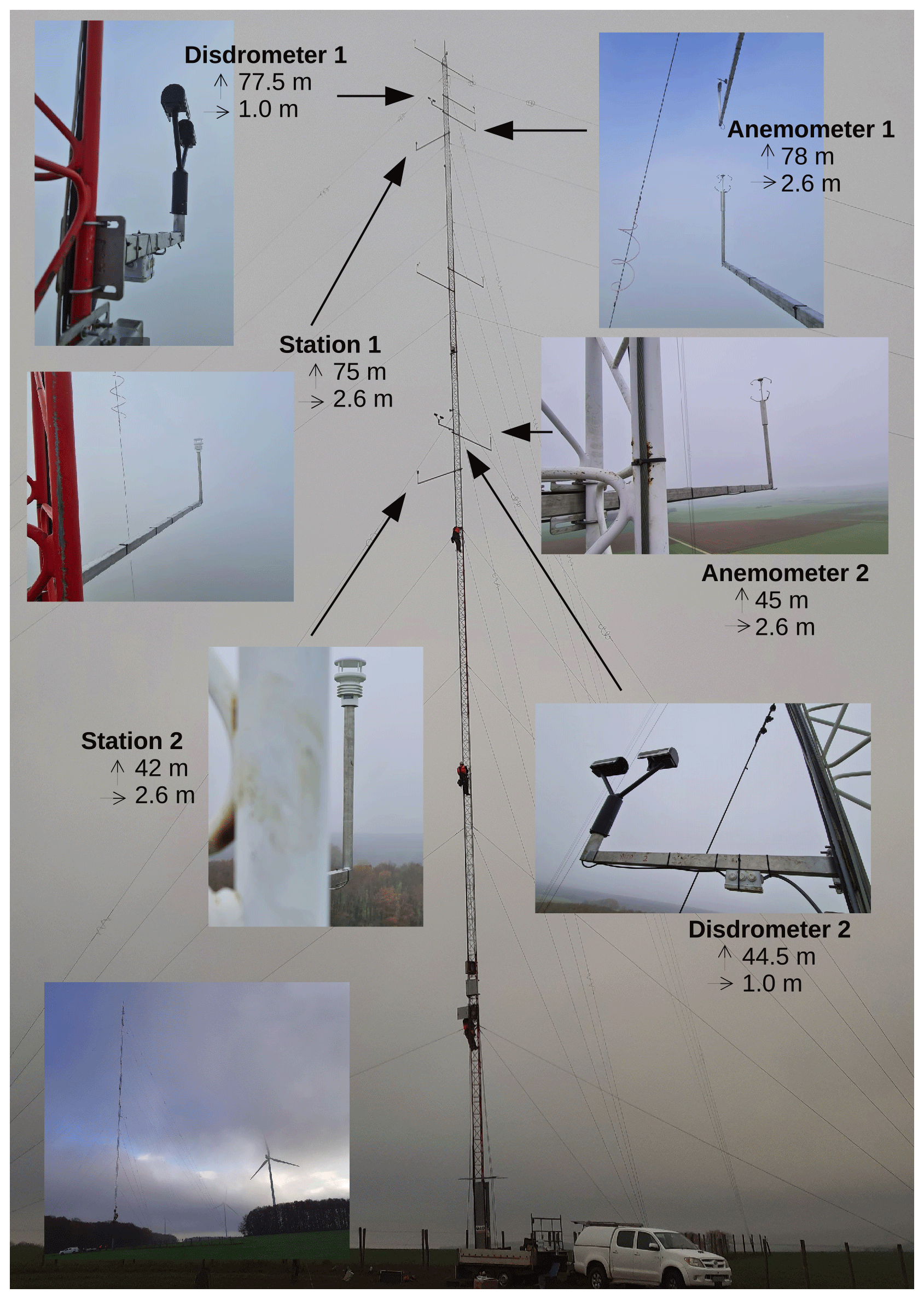
Figure 5 exhibits a picture of a meteorological mast along with the six devices installed on it. More precisely, at approximately 78 m, a 3D sonic anemometer, a mini meteorological station, and a disdrometer are installed. The same setting is repeated at roughly 45 m. The precise elevation and offset from the mast of the six devices are indicated on near the corresponding magnified pictures in Fig. 5. The two Raspberry Pi computers, which are collecting data along with the 4G modem enabling us to access data remotely, are located in one of the boxes at roughly 10 m.
2.2 The 3D sonic anemometers and associated outputs
We used two 3D sonic anemometers manufactured by Thies Clima (ThiesCLIMA, 2013a) in this measurement campaign. A 3D sonic anemometer is made of three pairs of transducers. Let us denote L as the distance between two transducers and uL as the wind velocity along the corresponding axis. The transducers can be either transmitters or receivers of a sound pulse, and they constantly swap roles. It means that the device actually measures the travel time of a pulse of sound between the two transducers in one direction or the other. If these times are denoted by t1 and t2, we have and , with c being the local speed of sound in the air; this yields the following:
which does not depend on c. The wind velocity is assessed along the axis between each three pairs, enabling us to reconstruct 3D wind.
It is also possible to estimate c from the following:
Since c mainly depends on the local temperature T, the latter can be derived using standard relationships assuming a dry air. This yields a virtual sonic temperature. Additional corrections can be implemented to derive a corrected temperature accounting for relative humidity and pressure (see ThiesCLIMA, 2013a, for more details). Hence, the 3D anemometers provide 3D wind measurement along with an estimate of temperature. The sampling rate used in this campaign is of 100 Hz for these devices.
2.3 Meteorological station and associated outputs
We used two mini meteorological stations manufactured by Thies Clima (ThiesCLIMA, 2013b) in this measurement campaign. They give access to the most relevant meteorological parameters, i.e. wind velocity and direction, air temperature, relative humidity, precipitation, and brightness. The sampling rate used in this campaign is of 1 Hz for these devices.
The wind information is obtained thanks to a 2D sonic anemometer made of two pairs of transducers positioned perpendicularly in relation to each other. See Sect. 2.2 for more details on the functioning of such device. Built-in sensors are dedicated to measurement of air temperature and relative humidity. The measurement of pressure relies on a microelectromechanical system. The latter three are protected within a shelter. Precipitation intensity is estimated with the help of a mini Doppler radar. The signal reflected back by the hydrometeor is analysed, and a rain rate is derived relying on strong assumptions of the DSD shape and the relation between the size and velocity of drops. Brightness is measured with the help of four photo sensors, whose spectral sensitivity curve is tuned to the human eye's sensitivity. In addition, there is a GPS sensor.
2.4 Disdrometer and associated outputs
We used two OTT Parsivel2 disdrometers (OTT, 2014) in this measurement campaign. OTT is the name of the manufacturer. Such a device gives access to the size and velocity of the drops passing through its sampling area. The data regarding the disdrometer are actually similar to the data already discussed in Gires et al. (2018). Hence, the interested reader is referred to this paper and references therein for a detailed presentation of the devices and associated output. It will only be reiterated here that the main output of the disdrometer is actually a matrix with the number of drops recorded (ni,j) during the time step Δt (30 s here), according to the classes of equivolumic diameter (index i and defined by a centre Di and a width ΔDi expressed in mm) and fall velocity (index j and defined by a centre vj and a width Δvj expressed in m s−1). From this matrix, it is possible to derive any rainfall-related quantity and, notably, the following:
-
The rain rate R (in mm h−1).
-
The drop size distribution (DSD) N(D) (in m−3 mm−1), where N(D)dD is the number of drops per unit volume (in m−3), with an equivolumic diameter between D and D+dD (in mm). Given the binned nature of the disdrometer data, it is a discrete DSD, denoted as N(Di), that is actually computed. Many quantities relevant to researchers and practitioners can actually simply be expressed as moments of the DSD.
The table for the classes of diameter and velocity, the formulas for computing R and N(Di) and associated moments, and the filters imposed can be found in Gires et al. (2018) and are therefore not repeated here. Disdrometers have been widely used to measure rainfall, and examples of measurement comparisons among them and with rain gauges can be found in Miriovsky et al. (2004), Krajewski et al. (2006), Frasson et al. (2011), or Thurai and Bringi (2005), which are just a few examples.
2.5 Measurement period
The data presented in this paper were collected between 1 March 2020 and 31 May 2020. Over this 3-month period, there is a limited number of missing time steps with only 3840, 4237, 3691, 3734, 3658, and 3658 missing minutes for, respectively, anemometer no. 1, anemometer no. 2, station no. 1, station no. 2, disdrometer no. 1, and disdrometer no. 2. In the worst case, it corresponds to approximately 3 % of the time. They mainly correspond to periods of power outages on the mast, which turns off the devices and the computer retrieving the data. They are mainly short (a few minutes) power cuts, except on 8–10 March during which the power remained out for more than 2 d. A few more minutes are missing with the anemometers. This is likely because of the sporadic loss of information by the retrieving computer due to the high sampling frequency.
Figure 6 displays the rain rate and cumulative rainfall depth vs. time during the 3-month period (first row). The two disdrometers give very close estimates (159 mm for no. 1 and 157 mm for no. 2), with a difference smaller than 1.6 %. The two meteorological stations have a stronger difference between them (119 vs. 130 mm, hence roughly 9 % difference) and yield significantly smaller total rainfall depth. The difference, on average, is 24 % between the disdrometers and the stations. Such a difference is likely to be due to the fact that both devices rely on completely different measurement techniques. It should definitely be explored further in future investigations. The 1 min average total horizontal wind from the four measuring devices is displayed in the lower left panel of Fig. 6. In the area, daily average wind is higher in winter, with values up to 7.5 m s−1, and lower in summer, with minimum values of 4.5 m s−1. These values were obtained using 30 years of 50 m height wind from the MERRA (Modern-Era Retrospective Analysis for Research and Applications) data, which is a NASA reanalysis tool (Bosilovich et al., 2016; Gelaro et al., 2017). The available period has an average wind of 6 m s−1, which is consistent with usual values, although such an average fully neglects the variability, which is what this data set enables to study. Finally, the wind rose for the entire period is in right panel of Fig. 6. It can be seen that the wind is mainly oriented along a south–west/north–east axis.
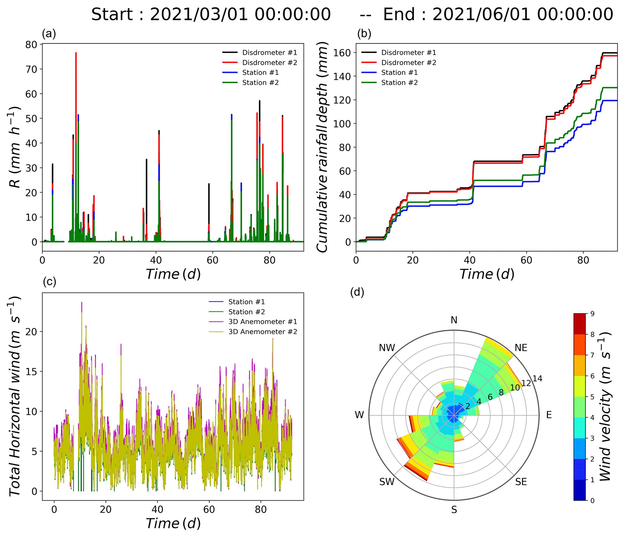
Figure 6Rain rate (a) and cumulative rainfall depth (b) vs. time over the 3 months of the measurement campaign, retrieved from the two disdrometers and the two meteorological stations. We use 1 min average wind (c) and a wind rose (d) computed from the 3D sonic anemometer no. 1, which is located at the top of the mast.
In this section, a detailed description of the database content and of some available basic scripts is provided. The overall organization is first described before providing some details on the Calendar_RW_Turb_wind_farm folder and the format of the files for each device.
3.1 Overall organization
The structure of the database is actually inherited from the data management flow, which is basically similar for all the devices.
-
Raw data are initially collected in the form of txt files corresponding directly to the outputs of the device. The data are stored in files corresponding to 1 min of data for stations and anemometers and 30 s for disdrometers.
-
All of these files are then zipped for individual days and stored in a corresponding folder in Raw_data_zip/.
-
These raw files are then used to generate daily (30 s or 1 Hz) or hourly (100 Hz for anemometer) files in an easy-to-read format. The csv files, then zipped to limit their size) are used for stations and anemometers. The npy files are used for Parsivel. They are stored in the corresponding folders of the database for which the name is quite explicit.
-
It is these files and not the raw ones that are used by the Python scripts to extract the data according to the user's needs.
Hence, the following structure was adopted for the database:
-
Data_base_rw_turb/
-
Raw_data_zip/
-
Anemometer_1/
-
Anemometer_2/
-
Station_1/
-
Station_2/
-
Pars_RW_turb_1/
-
Pars_RW_turb_2/
-
Each folder contains the files for its devices.
-
The name is
Raw_DeviceName_YYYYMMDD.zip (e.g. Raw_Anemometer_1_20210318.zip).
-
-
Daily_data_python_disdrometer/
-
Pars_RW_turb_1/
-
Pars_RW_turb_2/
-
Each folder contains the files for its disdrometers.
-
The name is
DisdroName_raw_data_YYYYMMDD.npy (e.g. Pars_RW_turb_1_raw_data_20210318.npy).
-
-
Daily_data_1Hz/
-
Anemometer_1/
-
Anemometer_2/
-
Station_1/
-
Station_2/
-
Each folder contains the files for its device.
-
The name is
Daily_data_1Hz_DeviceName_YYYYMMDD.csv (e.g. Daily_data_1Hz_Station_2_20210318.csv), which is zipped after.
-
-
Hourly_data_100Hz/
-
Anemometer_1/
-
Anemometer_2/
-
Each folder contains the files for its device.
-
The name is
Hourly_data_100Hz_DeviceName_YYYYMMDD _HH.csv
-
(e.g. Hourly_data_100Hz_Anemometer_2_ 20210318_07.csv), which is zipped after.
-
-
Calendar_RW_Turb_wind_farm
-
Data_30_sec/ (one file per day; e.g. R_30_sec_RW_Turb_wind_farm_2021_03_18 _00_00_00__2021_03_19_00_00_00.csv)
-
Quicklooks/ (one file per day; e.g. Quicklook_RW_Turb_wind_farm_2021_03_18_00 _00_00__2021_03_19_00_00_00.png)
-
Calendar_RW_Turb_wind_farm.html
-
-
Python_scripts/
-
The Python scripts (and associated files) to generate and use this database are located in this folder.
-
-
Read_me.txt
-
It contains a short description of the RW-Turb database.
-
-
3.2 Calendars
The purpose of this folder is to provide the user with a rapid access to a visual overview of the available data and enable the user to easily identify relevant periods/days according notably to the rainfall conditions. This is done through an html file (Calendar_RW_Turb_wind_farm.html) which contains links to a daily quick look and provides a rapid overview of the measurement campaign. Figure 7 displays a snapshot of it. Since the mentioned links are relative ones, the file should be located as indicated in the above structure for a proper functioning. Figure 8 shows an example of a daily quick look. It provides a summary of the recorded weather conditions with the following (explained from top to bottom and left to right in a given row):
-
Panel (a) shows rain rate vs. time.
-
Panel (b) shows cumulative rainfall depth vs. time.
-
Panel (c) shows an indication of the missing data, if any. Each line corresponds to a device. We used 1 min time steps.
-
Panel (d) shows DSD N(D) vs. time.
-
Panel (e) shows total horizontal wind ( vs. time for the various available devices. We used 1 min time steps.
-
Panel (f) shows temperature (∘C) vs. time with the various available data. We used 1 min time steps.
-
Panel (g) shows a representation of the number of drops according the velocity and size classes for the whole event. A solid black line corresponding to a standard relation (Lhermitte, 1988) between the terminal fall velocity of drops and their equivolumic diameters was added.
-
Panel (h) shows a wind rose using the horizontal wind measurements (ux and uy) of the two 3D sonic anemometers.
-
Panel (i) shows pressure (hPa) vs. time from the two meteorological stations. We used 1 min time steps.
-
Panel (j) shows N(D)D3 as a function of D (lower left). N(D)D3 is plotted, and not simply N(D), because it is basically proportional to the volume of rain obtained according to the drop diameter. Hence, it provides the reader with a better immediate insight of the influence of the various drops size on the observed rainfall event).
-
Panel (k) shows vertical wind (uz) vs. time from the two 3D sonic anemometers. We used 1 min time steps.
-
Panel (l) shows relative humidity (%) vs. time from the two meteorological stations. We used 1 min time steps.
All the daily quick look are stored in the folder Quicklooks and can be accessed directly there. For ease of access, the file name is simply Quicklook_RW_Turb_wind_farm_ followed by the date of start and end of the corresponding day in string format. For example, the one displayed in Fig. 8 is called Quicklook_RW_Turb_wind_farm_2021_05_06_00_00_00 __2021 _05_07_00_00_00.png. Local times are used.
Finally, the folder Data_30_sec/ contains daily rain rate files with the rain rate (in mm h−1) stored for each 30 s time step of the day in a csv file format. They are named in a similar way as to the Quicklook files
(e.g. R_30_sec_RW_Turb_wind_farm_2021_03_18 _00_00_00__2021_03_19_00_00_00.csv).
The format is straightforward, with (i) one line per 30 s time step starting on YYYY-MM-DD at 00:00:00 (UTC time). (ii) In each line, the values for the two disdrometers are separated with a semicolumn (the order is Pars no. 1; Pars no. 2), and (iii) missing data are noted as “nan”.
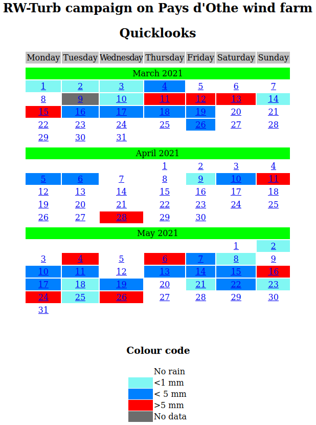
Figure 7Snapshot of the calendar summarizing the March–May 2021 measurement campaign on the meteorological mast of the Pays d'Othe wind farm.
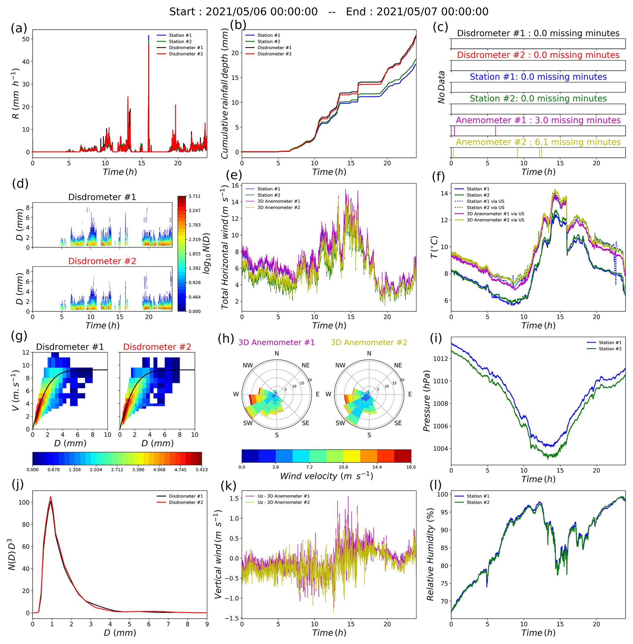
Figure 8Quick look of the meteorological data available on 6 May 2021. A precise description of each panel is given in the text.
3.3 3D anemometer data
The raw data are made of one txt file per minute directly containing the output telegram of the device. They are called Raw_DeviceName_YYYYMMDD_HHMM.txt. Such a file is made of 6000 lines, corresponding to 1 min, at a sampling rate of 100 Hz, and having the following format: b'02+000.03;-000.02;-000.01;+22.9;0E;47∘03', where the 3D wind is given, followed by the virtual sonic temperature and two status codes of the device. These files are then zipped per day and stored in the corresponding folder Raw_data_zip/.
Finally, some csv files containing all the relevant data are generated for each device. Hourly files are used for the data at 100 Hz and daily files for the data at 1 Hz (obtained simply by averaging 100 successive time steps). They are then stored in the corresponding folder of the database (see Sect. 3.1) in a zipped format to reduce their size.
The format is straightforward, with one line per each time step (0.01 or 1 s), and the four quantities of interest are separated with a semicolon, i.e. ux (m s−1); uy (m s−1); uz (m s−1); T (∘C). The x axis is oriented toward the east of the device, the y toward the north, and the z upward. Missing data are noted as nan.
3.4 Meteorological station data
The raw data are made of one txt file per minute directly containing the output telegram of the device. They are called Raw_DeviceName_YYYYMMDD_HHMM.txt. Such a file is made of 60 lines, corresponding to 1 min at a sampling rate of 1 Hz, and having the following format: b'00.01;000.0;+24.6;21062;21043;21060;21043;99;0;+23.0; +24.5;030.0;030.8;1025.8;000382;000809;000329;000282; 000809; 000;0000.569;1;+25.1;35.9;7297003;+48.842293; +002.588063;0148;038.7;169.2;13.03.20;11:25:47*13∘', where all the data are reported and separated by semicolon (see next paragraph for the order). These files are then zipped per day and stored in the corresponding folder, Raw_data_zip/, to reduce their size.
Finally, some daily csv files containing all the data are generated for each device. They are then stored in the corresponding folder of the database (see Sect. 3.1). The format is (i) one line per 1 s time step starting on YYYY-MM-DD at 00:00:00 (UTC time). (ii) In each line, values of measurement are provided separated by semicolon, and (iii) Missing data are noted as nan. In each line, the order of the data is as follows:
-
wind speed (m s−1)
-
wind direction (∘; starting clockwise from the north of the device)
-
virtual temperature (∘C)
-
propagation time converter 3 towards converter 1 (south to north)
-
propagation time converter 4 towards converter 2 (west to east)
-
propagation time converter 1 towards converter 3 (north to south)
-
propagation time converter 2 towards converter 4 (east to west)
-
measured value buffer content level 0 %… 99 %
-
heating requirement
-
calculated air temperature (∘C)
-
temperature uncompensated (∘C)
-
relative humidity uncompensated (%)
-
calculated relative humidity (%)
-
air pressure (hPa)
-
brightness north (lux)
-
brightness east (lux)
-
brightness south (lux)
-
brightness west (lux)
-
brightness max. value/vectorial sum (lux; s. Command BO)
-
direction of brightness (∘)
-
precipitation intensity (mm h−1)
-
precipitation event (0/1)
-
temperature in housing (∘C)
-
supply voltage (V)
-
internal counter (ms)
-
latitude (∘)
-
longitude (∘)
-
height of sensor referred to sea level (m)
-
position of the Sun, elevation (∘; −90… +90∘ = zenith)
-
position of the Sun, azimuth (∘; 0∘ = north; 180∘ = south).
3.5 Disdrometer data
As for the other devices, the raw data are made of one txt file per 30 s time step containing all the collected data. It should be stressed that it corresponds to the raw data and is made available for expert users only. Most users will not need to access them and will be satisfied with the provided Python scripts. The precise format for these raw fields can be found in the Python scripts with the heading of corresponding functions.
Finally, a daily file containing a list of the data collected by the devices for each time step is generated and stored on the corresponding folder of Daily_data_python_disdrometer/. They are stored in npy format and are readable with the help of Python 3. The Python scripts made available actually use these files. More precisely, each element of the list corresponds to a time step of 30 s. Each element of the list is again a list containing these elements (in the same order):
-
0 is the sensor ID.
-
1 is the precipitation rate (mm h−1) computed by the device.
-
2 is the temperature in the sensor (∘C), which is a rough estimate used for control than as a meteorological measurement.
-
3 is the OTT standard size/velocity map, i.e. a 32×32 matrix containing the number of drops recorded according to classes of size and velocity. Rows correspond to classes of size, while columns correspond to classes of velocity.
3.6 Python_scripts/
This section presents some Python scripts that are designed to enable the user carry out some initial analysis and basic data treatment with the database. The functions, which are basic toolboxes, can be found in the script Tools_overall_management_RW_Turb_data_paper.py. The main functions are as follows (only a short description is given here; more details, including precise description of the inputs and outputs of the functions, are provided as comments inside each script):
-
Quicklook_RW_Turb_wind_farm generates a quick look image and the corresponding 30 s and 5 min rain rate time series for a given rainfall event during the measurement campaign on the wind farm.
-
extracting_one_event_Parsivel reads daily npy files and generates a list containing all the data that can be analysed.
-
extracting_one_event_anemometer_100Hz reads daily files at 100 Hz and generates a matrix with the data for a given anemometer and event.
-
extracting_one_event_anemometer_1Hz reads daily files at 1 Hz and generates a matrix with the data for a given anemometer and event.
-
extracting_one_event_station_1Hz reads daily files at 1 Hz and generates a matrix with the data for a given station and event.
Examples for use of the various functions can be found in the scripts Script_overall_management_parsivel_v1.py, Script_overall_management_station_v1.py, Script_overall_management_anemometer_v1.py, and Script_overall_management_RW_Turb_campaign_v1.py. On a standard laptop, it typically takes few seconds to extract and display all the data for 1 d.
The data from a 3-month measurement campaign with devices installed on a meteorological mast of Boralex located at the wind farm of Pays d'Othe are presented in this paper. Raw data along with Python-formatted data with corresponding scripts are described. The Hydrology Meteorology and Complexity laboratory of École des Ponts ParisTech (HM&Co-ENPC) has made this data set available at https://doi.org/10.5281/zenodo.5801900 (Gires et al., 2021). The following citation should be used for every use of the data:
-
For this paper, https://doi.org/10.5194/essd-2021-463.
-
For the database, Gires, A., Jose, J., Tchiguirinskaia, I., and Schertzer, D.: Data for: “Three months of combined high resolution rainfall and wind data collected on a wind farm”, Zenodo [data set], https://doi.org/10.5281/zenodo.5801900, 2021.
This data set is available for download free of charge. License terms apply. The campaign is actually still ongoing. Regular updates of its status, along with updates of the database, are to be provided through the lab's website (http://hmco.enpc.fr, last access: 16 August 2022). The web page https://hmco.enpc.fr/portfolio-archive/rw-turb/ (last access: 16 August 2022) already contains links to the summary calendars for past and ongoing measurement campaigns (daily updates). The database will continue to be organized as presented in this paper, and users interested in a longer series, once available, can contact the corresponding author.
While studying the small-scale space–time fluctuations, it is advantageous to use data at the finest available resolution. However, it is possible that the actual sampling resolution may be different due to quality problems in the series, leaving spurious estimates at finer scales. To understand this, 100 Hz data from anemometers and 1 Hz data from meteorological station were analysed using spectral analysis and the framework of universal multifractals (UMs).
Spectral analysis is a commonly used technique in turbulence to estimate scaling behaviour using second order statistics. In the case of scaling behaviour, power spectrum E(k) and frequency are power law related, as follows:
where k is the corresponding frequency, and β is the spectral exponent (slope in log-log plot).
In the universal multifractal (UM) framework, all moment orders are used and not only the moment order 2 as in spectral analysis. This enables us to capture information over a larger spectrum from higher-order moments, which emphasize on extremes, to small-order moments focusing on smaller values. In this framework, we have the following:
where ϵλ is the studied conservative field at resolution λ (i.e. the ratio of largest scale to observation scale) and K(q) the moment scaling function at moment order q (Schertzer and Lovejoy, 1987, or Schertzer and Tchiguirinskaia, 2020, for a recent review). K(q) fully characterizes the variability across scales of the studied field. In the UM framework, K(q) is fully determined with the help of only two UM parameters, i.e. the mean intermittency co-dimension C1 and multifractality index α. C1 measures mean intermittency in the field; when C1=0, the field is homogeneous with little variability. α quantifies how much this intermittency changes when moving away from the average behaviour. ; the higher the value of α, the higher the variability, with α=0 being a monofractal field where an extreme intermittency is the same as that of mean. A multifractal analysis of collected data is performed to check for the effective resolution of the data, i.e. to assess if measurements are affected or not by instrumental artefacts at small scales. Given the stated purpose, only small scales (i.e. from 16 s down to 0.01 s) are studied here. Analysis and interpretation of larger-scale regimes will be carried out in further scientific papers.
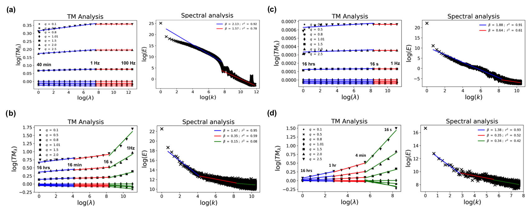
Figure 9TM analysis (Eq. 4 in log-log plot), and spectral analysis (Eq. 3 in log-log plot) of 1 month long data (27 January to 27 February 2021) for (a) anemometer data at 100 Hz (sample length of 40 min), (b) fluctuations of anemometer data at 1 Hz (sample length of 16 h), (c) Temperature (T) at 1 Hz (sample length of 16 h), (d) fluctuations of Temperature (T) at 15 s (sample length of 16 h).
Spectral analysis, which consists of plotting Eq. (3) in log-log, and trace moment (TM) analysis, which consists of plotting Eq. (4) in log-log for various moments q, enable to confirm the scaling behaviour of studied fields. It is the case if straight lines are retrieved, potentially with several scaling regimes. The retrieved slopes give β for the spectral analysis and K(q) in the TM analysis. In Fig. 9a, trace moment (TM) analysis and a spectral analysis for 100 Hz anemometer data are shown (ensemble analysis of 1-month-long data – 1 March to 1 April 2021 – with a sample length of 40 min). Other periods have been tested and yielded similar results with regards to the effective resolution issue discussed in the framework of this data paper. A spectral spike is observed at frequency 0.0304 s−1, and spurious fluctuations are visible for small scales. The spike is due to the fact that at 100 Hz, the same data are basically repeated over three successive time steps. Estimates of UM parameters, obtained with the help of double TM analysis (a more robust form of TM tailored for UM fields), yield for the small-scale regime (1–100 Hz) values of C1 that are too low () to consider any variation in the field. As the field is too smooth here (high value of β: 2.13 and 1.57), as suggested by Lavallee et al. (1993), fluctuations were analysed by differentiating the field. This enables us to study an approximation of the underlying conservative fields (hence the decrease in estimates of β and H). In fluctuations of the same 100 Hz of data, nearly 70 % of the values are equal to zero, which results in strong bias for estimates with an artificial decrease of α (=0.31 here) and an increase in C1 (=0.21 here), which is consistent with bias associated with numerous zeros (Gires et al., 2012). This further suggests the possibility of having instrumental noise in resolutions finer than 1 Hz. It is unclear where exactly the scaling break is (close to 1 or 10 Hz) to consider instrumental noise, but to be on the safe side, we decided to take 1 Hz as the limiting value. An analysis of the fluctuations of 1 Hz data (ensemble analysis of 1-month-long data – 1 March to 1 April 2021 – with a sample length of 16 h) is shown in Fig. 9b. For the small-scale regime (1–16 s), we find α=1.49 and C1=0.09, which is more consistent with estimates commonly retrieved for atmospheric fields.
Similar results (extremely small values of C1 or β suggesting instrumental noise) are observed for other 1 Hz data available at meteorological stations, with temperature (T), pressure (P), humidity (RH), and air density (ρ, a function of T, P & RH) of 16 s being close to the actual effective sampling resolution. Figure 9c shows the TM analysis for T; on the basis of spectra, the second scaling regime (16 s to 1 Hz) seems to suggest presence of instrumental artefacts (ensemble analysis of 1-month-long data – 1 March to 1 April 2021 – with a sample length of 16 h). For the 1–16 s regime, we find α=1.99 and ; the low C1 supports the spectral observation. In 1 Hz station data, values of many data points were actually very close to each other, resulting again in the presence of a lot of zeroes in the fluctuations of the series (about 75 % for T fluctuations). This in turn gave biased estimates of both α and C1. Averaging data over time reduced this effect, and by considering fluctuations of data at 15 s, realistic values of α and C1 were retrieved (Fig. 9d; α=1.12 and C1=0.14 for 15 s–4 min scaling regime).
For analysing the fields' variability, it is worthwhile to note that the actual sampling resolution – the resolution from which fields can be studied to obtain consistent UM parameters – is not necessarily the lowest resolution of instrumental data availability. Indeed, it could be affected by instrumental artefacts (white noise and repeated values). Here, it is more realistic to study anemometer and station data at a coarser resolution (1 Hz and 16 s respectively) where it is exhibiting clear scaling variability than at the finest available resolution of data recording (100 and 1 Hz). The multifractal framework is a powerful tool to study this issue and assess the quality of the data.
AG, IT, and DS designed the measurement campaign. AG supervised the implementation of the measurement campaign and wrote a large part of the paper. JJ implemented the analysis of Sect. 5 and wrote it under the supervision of AG, IT, and DS. All authors contributed to the review of the paper.
The contact author has declared that none of the authors has any competing interests.
Publisher's note: Copernicus Publications remains neutral with regard to jurisdictional claims in published maps and institutional affiliations.
The authors would like to thank Boralex, and notably Ernani Schnorenberger, for facilitating access to the meteorological mast they are operating on the Pays d'Othe wind farm.
This work has been supported by the ANR JCJC RW-Turb project (grant no. ANR-19-CE05-0022).
This paper was edited by David Carlson and reviewed by two anonymous referees.
Al, B. C., Klumpner, C., and Hann, D. B.: Effect of Rain on Vertical Axis Wind Turbines. Proceedings of the International Conference on Renewable Energies and Power Quality, Las Palmas de Gran Canaria (Spain), 13 to 15 April 2011. a
Bosilovich, M. G., Lucchesi, R., and Suarez, M.: MERRA-2: File specification, GMAO Office Note No. 9 (Version 1.1), p. 73, http://gmao.gsfc.nasa.gov/pubs/office_notes (last access: 16 August 2022), 2016. a
Cai, M., Abbasi, E., and Arastoopour, H.: Analysis of the Performance of a Wind-Turbine Airfoil under Heavy-Rain Conditions Using a Multiphase Computational Fluid Dynamics Approach, Industrial & Engineering Chemistry Research, 52, 3266–3275, https://doi.org/10.1021/ie300877t, 2013. a
Cohan, A. C. and Arastoopour, H.: Numerical simulation and analysis of the effect of rain and surface property on wind-turbine airfoil performance, Int. J. Multiphas. Flow, 81, 46–53, https://doi.org/10.1016/j.ijmultiphaseflow.2016.01.006, 2016. a
Corrigan, R. and Demiglio, R.: Effect of Precipitation on Wind Turbine Performance, NASA TM-86986, 1985. a
Fitton, G., Tchiguirinskaia, I., Schertzer, D., and Lovejoy, S.: Scaling Of Turbulence In The Atmospheric Surface-Layer: Which Anisotropy?, J. Phys. Conf. Ser., 318, 072008, https://doi.org/10.1088/1742-6596/318/7/072008, 2011. a
Fitton, G., Tchiguirinskaia, I., Schertzer, D., and Lovejoy, S.: Torque Fluctuations In The Framework Of A Multifractal 23/9-Dimensional Turbulence Model, J. Phys. Conf. Ser., 555, 012038, https://doi.org/10.1088/1742-6596/555/1/012038, 2014. a
Frasson, R. P. D. M., da Cunha, L. K., and Krajewski, W. F.: Assessment of the Thies optical disdrometer performance, Atmos. Res., 101, 237–255, 2011. a
Gelaro, R., McCarty, W., Suárez, M. J., Todling, R., Molod, A., Takacs, L., Randles, C. A., Darmenov, A., Bosilovich, M. G., Reichle, R., Wargan, K., Coy, L., Cullather, R., Draper, C., Akella, S., Buchard, V., Conaty, A., da Silva, A. M., Gu, W., Kim, G.-K., Koster, R., Lucchesi, R., Merkova, D., Nielsen, J. E., Partyka, G., Pawson, S., Putman, W., Rienecker, M., Schubert, S. D., Sienkiewicz, M., and Zhao, B.: The Modern-Era Retrospective Analysis for Research and Applications, Version 2 (MERRA-2), J. Climate, 30, 5419–5454, https://doi.org/10.1175/JCLI-D-16-0758.1, 2017. a
Gires, A., Tchiguirinskaia, I., Schertzer, D., and Lovejoy, S.: Influence of the zero-rainfall on the assessment of the multifractal parameters, Adv. Water Resour., 45, 13–25, https://doi.org/10.1016/j.advwatres.2012.03.026, 2012. a
Gires, A., Tchiguirinskaia, I., and Schertzer, D.: Drop by drop backscattered signal of a m3 volume: A numerical experiment, Atmos. Res., 178–179, 164–174, https://doi.org/10.1016/j.atmosres.2016.03.024, 2016. a
Gires, A., Tchiguirinskaia, I., and Schertzer, D.: Two months of disdrometer data in the Paris area, Earth Syst. Sci. Data, 10, 941–950, https://doi.org/10.5194/essd-10-941-2018, 2018. a, b
Gires, A., Jose, J., Tchiguirinskaia, I., and Schertzer, D.: Data for: “Three months of combined high resolution rainfall and wind data collected on a wind farm”, Zenodo [data set], https://doi.org/10.5281/zenodo.5801900, 2021. a, b
Krajewski, W. F., Kruger, A., Caracciolo, C., Golé, P., Barthes, L., Creutin, J.-D., Delahaye, J.-Y., Nikolopoulos, E. I., Ogden, F., and Vinson, J.-P.: DEVEX-disdrometer evaluation experiment: Basic results and implications for hydrologic studies, Adv. Water Resour., 29, 311–325, 2006. a
Lavallee, D., Lovejoy, S., Schertzer, D., Ladoy, P., De Cola, L., and Lam, N.: Nonlinear variability and landscape topography: analysis and simulation, in: Fractals in geography, edited by: de Cola, L. and Lam, N., 171–205, Englewood Cliffs, Prentice-Hall, 1993. a
Lhermitte, R. M.: Cloud and precipitation remote sensing at 94 GHz, Geoscience and Remote Sensing, IEEE Transactions on, 26, 207–216, 1988. a
Miriovsky, B. J., Bradley, A. A., Eichinger, W. E., Krajewski, W. F., Kruger, A., Nelson, B. R., Creutin, J.-D., Lapetite, J.-M., Lee, G. W., Zawadzki, I., and Ogden, F. L.: An Experimental Study of Small-Scale Variability of Radar Reflectivity Using Disdrometer Observations, J. Appl. Meteorol., 43, 106–118, https://doi.org/10.1175/1520-0450(2004)043<0106:AESOSV>2.0.CO;2, 2004. a
OTT: Operating instructions, Present Weather Sensor OTT Parsivel2, 2014. a
Schertzer, D. and Lovejoy, S.: Physical modeling and analysis of rain and clouds by anisotropic scaling multiplicative processes, J. Geophys. Res.-Atmos., 92, 9693–9714, https://doi.org/10.1029/JD092iD08p09693, 1987. a
Schertzer, D. and Tchiguirinskaia, I.: A Century of Turbulent Cascades and the Emergence of Multifractal Operators, Earth Space Sci., 7, e2019EA000608, https://doi.org/10.1029/2019EA000608, 2020. a
ThiesCLIMA: 3D Ultrasonic anemometer, Instructions for use, 2013a. a, b
ThiesCLIMA: Clima sensor US, Instructions for use, 2013b. a
Thurai, M. and Bringi, V. N.: Drop Axis Ratios from a 2D Video Disdrometer, J. Atmos. Ocean. Tech., 22, 966–978, https://doi.org/10.1175/JTECH1767.1, 2005. a
van Kuik, G. A. M., Peinke, J., Nijssen, R., Lekou, D., Mann, J., Sørensen, J. N., Ferreira, C., van Wingerden, J. W., Schlipf, D., Gebraad, P., Polinder, H., Abrahamsen, A., van Bussel, G. J. W., Sørensen, J. D., Tavner, P., Bottasso, C. L., Muskulus, M., Matha, D., Lindeboom, H. J., Degraer, S., Kramer, O., Lehnhoff, S., Sonnenschein, M., Sørensen, P. E., Künneke, R. W., Morthorst, P. E., and Skytte, K.: Long-term research challenges in wind energy – a research agenda by the European Academy of Wind Energy, Wind Energ. Sci., 1, 1–39, https://doi.org/10.5194/wes-1-1-2016, 2016. a
Walker, S. and Wade, J.: Effect of precipitation on wind turbine performance, DOE DE1IOO1144, 1986. a