the Creative Commons Attribution 4.0 License.
the Creative Commons Attribution 4.0 License.
 | 17 Aug 2022
QUADICA: water QUAlity, DIscharge and Catchment Attributes for large-sample studies in Germany
Rohini Kumar
Stefanie R. Lutz
Tam Nguyen
Fanny Sarrazin
Michael Weber
Olaf Büttner
Sabine Attinger
Andreas Musolff
Environmental data are the key to defining and addressing water quality and quantity challenges at the catchment scale. Here, we present the first large-sample water quality data set for 1386 German catchments covering a large range of hydroclimatic, topographic, geologic, land use, and anthropogenic settings. QUADICA (water QUAlity, DIscharge and Catchment Attributes for large-sample studies in Germany) combines water quality with water quantity data, meteorological and nutrient forcing data, and catchment attributes. The data set comprises time series of riverine macronutrient concentrations (species of nitrogen, phosphorus, and organic carbon) and diffuse nitrogen forcing data (nitrogen surplus, atmospheric deposition, and fixation) at the catchment scale. Time series are generally aggregated to an annual basis; however, for 140 stations with long-term water quality and quantity data (more than 20 years), we additionally present monthly median discharge and nutrient concentrations, flow-normalized concentrations, and corresponding mean fluxes as outputs from Weighted Regressions on Time, Discharge, and Season (WRTDS). The catchment attributes include catchment nutrient inputs from point and diffuse sources and characteristics from topography, climate, land cover, lithology, and soils. This comprehensive, freely available data collection with a large spatial and temporal coverage can facilitate large-sample data-driven water quality assessments at the catchment scale as well as mechanistic modeling studies. QUADICA is available at https://doi.org/10.4211/hs.0ec5f43e43c349ff818a8d57699c0fe1 (Ebeling et al., 2022b) and https://doi.org/10.4211/hs.88254bd930d1466c85992a7dea6947a4 (Ebeling et al., 2022a).
- Article
(9351 KB) - Full-text XML
- BibTeX
- EndNote


Understanding hydrological and biogeochemical processes at various spatiotemporal scales is a major goal in catchment hydrology and is particularly relevant for robust predictions of water quantity and quality as well as adequate catchment management. Analyzing observations of the spatial and temporal dynamics of water quantity and quality at the catchment scale can give insights into relevant processes using a “pattern to process” approach (Sivapalan, 2006). Especially large-sample studies covering a wide range of catchments can advance our knowledge on patterns across scales, catchment similarity, and dominant processes, beyond a single catchment or local behavior (Addor et al., 2020; Kingston et al., 2020). Such studies allow for generalizable theories and applications by “balancing depth with breadth” and facilitate classifications, regionalization, and a better understanding of uncertainty in model predictions (Gupta et al., 2014). Thus, environmental data are the key for process understanding and hypothesis testing (Li et al., 2021). The collection and availability of water quantity and quality data are steadily increasing with technological advances (Rode et al., 2016), but particularly harmonized and quality-controlled large-sample data sets of water quality and quantity along with catchment attributes are needed. These enable the identification and characterization of water quality and quantity response patterns and relationships with potential controls, facilitate hypothesis testing, and, thus, advance our understanding of the complex coupled hydrological and biogeochemical systems across larger samples and domains (Li et al., 2021).
In recent years, the application of large-sample studies has been advancing fast for (surface) water quantity studies investigating dominant processes and drivers of water flow characteristics. Gupta et al. (2014) provided an overview of such studies, with the first of them being published in the 1990s. These publications have been followed by a recent surge in studies documenting and analyzing large-sample hydrologic data sets, such as Newman et al. (2015), Kuentz et al. (2017), Do et al. (2017), Gnann et al. (2020), Tarasova et al. (2020), and Merz et al. (2020). These studies have identified catchment typologies, archetypal behavior, and underlying controls, such as discharge variability across Europe (Kuentz et al., 2017), catchments with similar runoff event types (Tarasova et al., 2020), or how catchment discharge attenuates and shifts climate seasonality (Gnann et al., 2020).
In contrast, large-sample studies for water quality are less common. Nevertheless, some recent large-sample water quality studies have provided a basis for enhancing our understanding of catchment functioning in terms of the mobilization, transport, and environmental fate of solutes and particulates as well as the generality of these functions. For example, Monteith et al. (2007) linked widespread positive trends in dissolved organic carbon (DOC) concentrations observed in Europe and North America with decreasing atmospheric sulfur and chloride deposition. Godsey et al. (2009, 2019) provided wide evidence that weathering-derived solutes are mostly exported chemostatically with low concentration variance. Basu et al. (2010) derived the hypothesis of chemostatic nutrient export resulting from homogenized sources due to the legacy of high inputs. More recently, Zarnetske et al. (2018) and Ebeling et al. (2021a) both provided evidence of widespread transport-limited DOC export from small to large catchments. However, several questions regarding general patterns, catchment similarities and typologies, and the underlying controls of the aforementioned factors remain open – for example, questions concerning the extent and recovery of nutrient legacy for both nitrogen (N) and phosphorous (P) (Chen et al., 2018), the extent of macronutrient interactions in differing landscape and anthropogenic settings as well as throughout the river network (Wollheim et al., 2018), and the impact of climate change on water quality trajectories in various catchments (Kaushal et al., 2018).
At the moment, large-sample studies are still hampered by limited availability (e.g., the number of stations, number of samples, and covered regions) and accessibility of spatially and temporally harmonized large-sample data collections (e.g., Addor et al., 2020), despite recent efforts to make consistent large-sample data sets of catchment hydrology for both water quantity and water quality in streams publicly available (e.g., Virro et al., 2021). Prominent examples of large-sample hydrological data sets including catchment attributes are the Catchment Attributes and MEteorology for Large-sample Studies (CAMELS) data sets, available for the USA (Addor et al., 2017), Chile (Alvarez-Garreton et al., 2018), Brazil (Chagas et al., 2020), Great Britain (Coxon et al., 2020), and Australia (Fowler et al., 2021). More recently, the multinational LArge-SaMple DAta for Hydrology and Environmental Sciences (LamaH; Klingler et al., 2021) initiative has provided hydrometeorological time series at an hourly resolution along with catchment attributes. For stream water quality, currently available large-sample data sets focus on water quality time series only but lack additional data. Recently, two global databases of surface water quality were published that combine data from several existing databases in homogenized and quality-checked form: the Surface Water Chemistry database (SWatCh; Rotteveel and Sterling, 2022), with a focus on variables relevant to acidification, and the Global River Water Quality Archive (GRQA; Virro et al., 2021), with a focus on macronutrients. Both include the global databases Global Freshwater Quality Database (GEMStat; UNEP, 2018) and the GLObal RIver CHemistry database (GLORICH; Hartmann et al., 2014) as well as the European Waterbase (EEA, 2020) database, although the spatiotemporal coverage of the data varies strongly. These are important recent advances towards open science in water quality research. However, to the authors' knowledge, there is currently no combined, ready-to-use data set of metrics of water quality, quantity, catchment attributes, and forcing data (such as meteorological and nutrient inputs), which would allow for the investigation of water quality dynamics and their controls. Moreover, large-sample and cross-regional studies are especially challenging in countries like Germany, where data responsibility is scattered between federal states and data are often not freely available nor homogenized between water quantity and quality stations. Nevertheless, a few Germany-wide water quality studies on groundwater (Knoll et al., 2020) and surface water (Ebeling et al., 2021a) have recently been carried out.
The key objective here is to provide a spatially and temporally consistent comprehensive data set of joint water quality and quantity data, catchment attributes, and nutrient inputs for German catchments that is ready to use and freely available, supporting the open science philosophy and FAIR (findability, accessibility, interoperability, and reuse) data principles. In this “Water QUAlity, DIscharge and Catchment Attributes for large-sample studies in Germany” (QUADICA) data set, we have complemented available data sets of catchment attributes with new data on water quality and water quantity. These data include delineated catchment boundaries, catchment responses in terms of macronutrient concentrations (species of N; P; and organic carbon, OC) and discharge (Q), forcing data in terms of meteorological and diffuse nitrogen inputs, and average catchment attributes. We distinguish stations with a high data availability, which allows further estimation of daily concentrations and fluxes using a regression approach, and stations with lower availability, for which aggregated observed concentrations are reported. For water quality (Sect. 3.1) and water quantity (Sect. 3.2), we provide the following:
-
time series of annual medians of observed macronutrient concentrations (dissolved and total forms of N, P, and OC) and of observed discharge,
-
time series of monthly and annual medians of estimated daily macronutrient concentrations and flow-normalized concentrations as well as mean nutrient fluxes and medians of observed discharge for stations with high data availability,
-
monthly medians and the monthly 25th and 75th percentiles of observed concentrations and discharge over the whole time series.
Additionally, we provide time series of driving forces (Sect. 3.3 and 3.4) and catchment attributes (Sect. 4):
- 4.
time series of observed monthly meteorological forcing variables as catchment averages (Sect. 3.3),
- 5.
time series of estimated annual net diffuse nitrogen inputs to the catchments (Sect. 3.4),
- 6.
average catchment attributes, i.e., topography, land cover, nutrient sources, lithology and soils, and hydroclimate (Sect. 4).
We envision that the QUADICA data set will directly enable large-sample assessments of mean concentrations and fluxes; their variability in terms of long-term trends, seasonality, and relationships to discharge; and their relationships to catchment attributes. We believe that the data set will allow a better understanding of catchment functioning and water management beyond regional scales and stimulate provisioning and analysis of further water quality data at national to continental scales.
The station selection and catchment delineation have been presented in a previous study (Ebeling et al., 2021a) and data repository (Ebeling, 2021) and are now included in the new QUADICA data set. All data sets use the same unique identifier (OBJECTID) for the stations and corresponding catchments. The station selection is based on riverine water quality data assembled from the German federal state environmental authorities, who are responsible for the routine monitoring of water quality in Germany (Musolff et al., 2020; Musolff, 2020) and take grab samples at approximately monthly intervals.
The following preprocessing steps were applied for each station and compound separately: we removed duplicate, negative, and zero values and applied an outlier test for each time series (removing values above mean concentration and 4 times the standard deviation in logarithmic space, i.e., confidence level >99.99 % for lognormally distributed data). Finally, 1386 stations met the criteria concerning water quality data and catchment delineation (Fig. 1) as described in the following: in the first step, water quality data cover at least 3 years, include a minimum of 70 samples from 2000 to 2015 after preprocessing, and cover all seasons, i.e., seasonal coverage of at least 10 % of the samples in each quarter considering all possible combinations of 3 consecutive months (criteria one to three as described in Ebeling et al., 2021a). These criteria should ensure that a representative amount of data is available. Stations fulfilling these water quality data criteria for nitrate (NO3-N) or phosphate (PO4-P) were preselected (i.e., 1692 stations). Other variables (e.g., total phosphorus, TP; total nitrogen, TN; and DOC) were not used in this initial step of station selection.
In the second step, we delineated the catchment area from topography for these preselected stations and verified them as described here. The topographic catchment boundaries were delineated based on a 100 m flow accumulation grid derived from a digital elevation model (DEM; resampled from 25 to 100 m using the average; EEA, 2013) using spatial analysis tools and a D8 flow direction type. The river network from the Rivers and Catchments of Europe – Catchment Characterisation Model (De Jager and Vogt, 2007) was used to burn by 10 m into the DEM before deriving the flow accumulation. The stations were snapped or manually moved towards the representative flow accumulation stream to define the catchment outlets (pour points). The resulting topography-based catchment polygons were quality-controlled manually by a comparison to the real river network. In case of major deviations, a few manual adaptations of the burned river segments were done if they substantially improved the overlap without hindering neighboring catchment delineations. In case of insufficient spatial overlap that could not be improved, stations were discarded from the selection. This resulted in a final set of 1386 catchments. The DEM, flow direction, and flow accumulation raster used as well as the modified station locations and the river network are also provided in the data repository for further use.
The varying density of stations across Germany (Fig. 1a) has two main reasons: firstly, the provision of raw data varied with respect to the number of stations, number of samples per compound and station, and time series length among the federal states; secondly, the topographic delineation of catchment boundaries was more successful where the topography is more pronounced, giving less delineable catchments in northern Germany. The delineated catchment boundaries are provided with the data set and enable the user to develop further geoinformation routines (e.g., to extract characteristics from other geographic data sets).
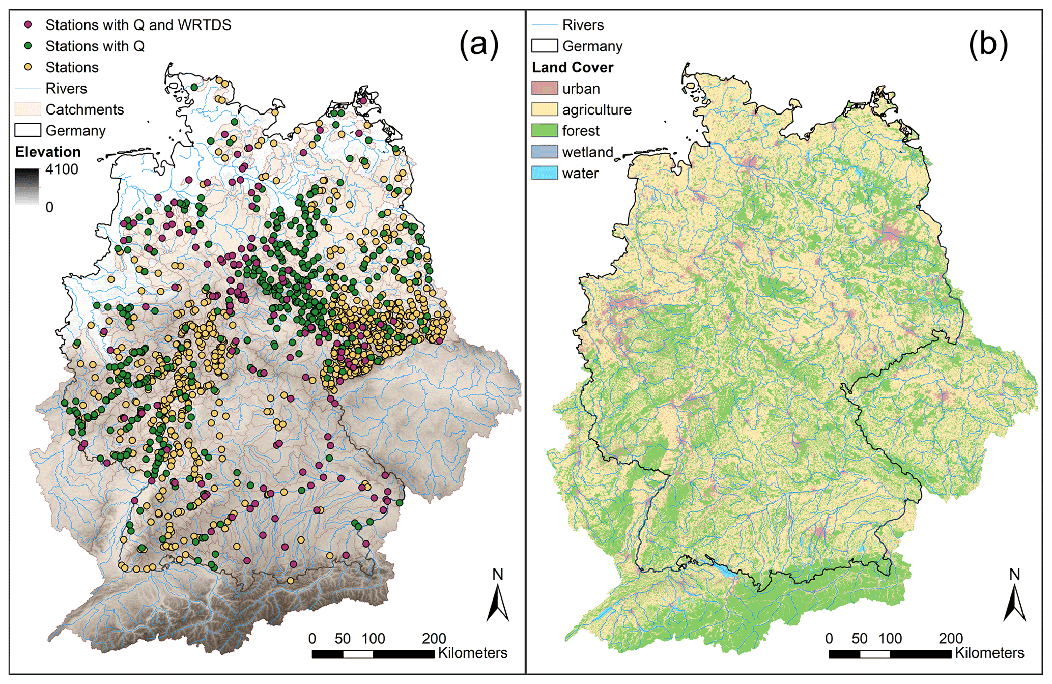
Figure 1Map of (a) water quality stations, catchments, and elevation (EEA, 2013) and (b) map of land cover (EEA, 2016a). The colors in panel (a) distinguish between stations with (green) and without (yellow) discharge (Q) data and stations with high data availability of concentration and discharge (purple, WRTDS stations; for details, see Sect. 3.1). WRTDS refers to Weighted Regressions on Time, Discharge, and Season.
For the 1386 delineated catchments, riverine concentration time series of nitrate (NO3-N), mineral nitrogen (Nmin), total nitrogen (TN), phosphate (PO4-P), total phosphorus (TP), dissolved organic carbon (DOC), and total organic carbon (TOC) are provided (Table 1). They are supplemented by time series of discharge (where available) and forcing variables (meteorological drivers and diffuse N input). Due to limited data availability, not all variables can be provided for all stations.
Table 1Provided time series data as well as their basis (observed or estimated), aggregation type, temporal resolution, and source of original data, which was used to calculate the aggregated data provided here.
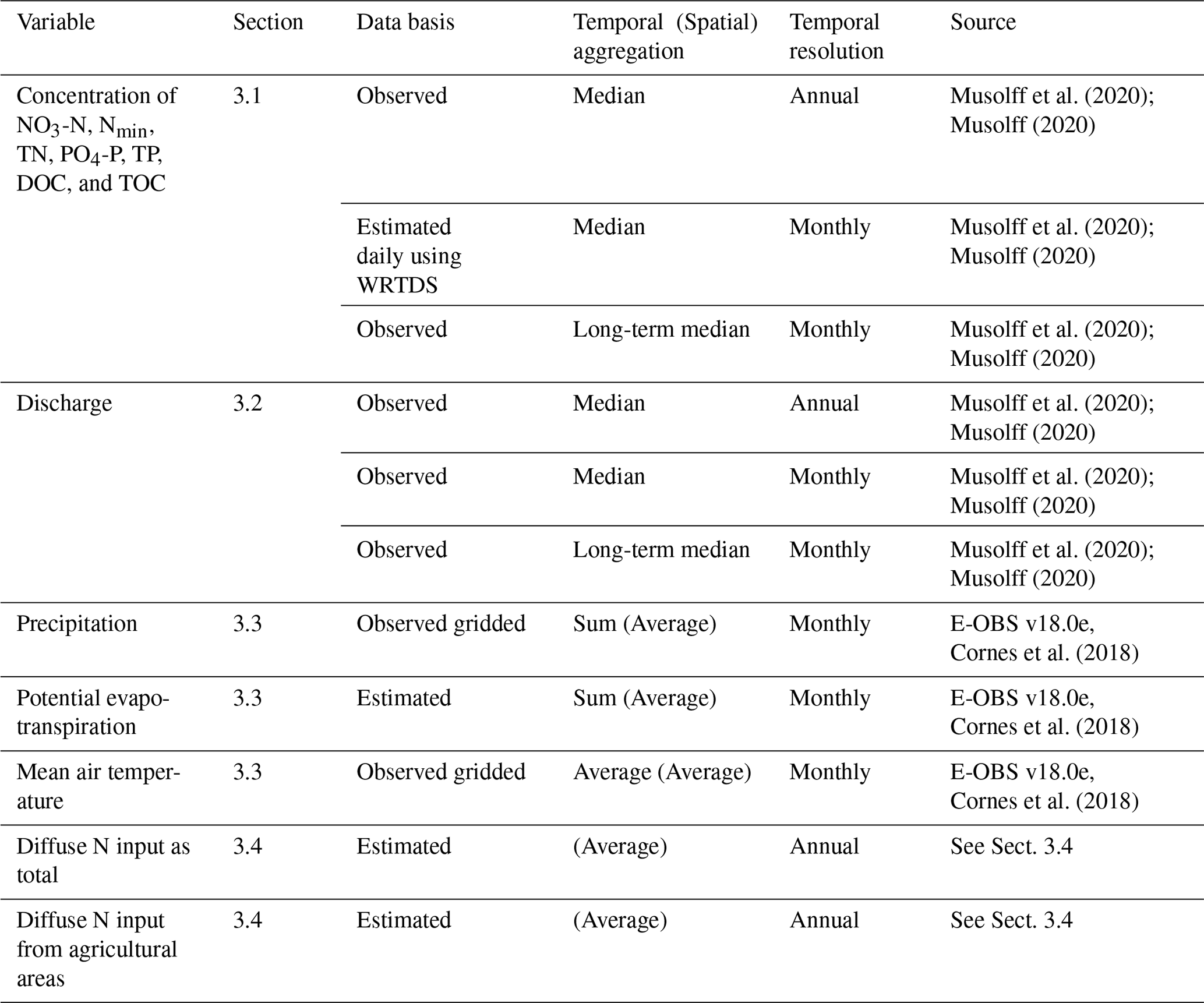
The abbreviations used in the table are as follows: nitrate (NO3-N); mineral nitrogen (Nmin); total nitrogen (TN); phosphate (PO4-P); total phosphorus (TP); dissolved organic carbon (DOC); total organic carbon (TOC); and Weighted Regressions on Time, Discharge, and Season.
3.1 Water quality time series
3.1.1 Annual median concentrations
Annual medians of concentration data are presented for time series of the 1386 stations fulfilling the water quality criteria (as done for the catchment selection criteria described in Sect. 2). To calculate summary statistics, we substituted concentration values below the detection limit (left-censored data) with half the detection limit.
The resulting data density distributions over time and the number of years covered by each variable show the highest data availability for TOC, PO4-P, and NO3-N in more recent years (Fig. 2). An overview of the time series statistics for each variable is given in Table 2, and time series are shown in Appendix A (Fig. A1). For NO3-N concentrations, the number of stations with available data is 1339, and the median number of samples per station is 157. The earliest time series starts in 1954, but the median start across stations is in 1994. The median time series length is 19 years, and the maximum time series length is 61 years. For PO4-P concentrations, the number of stations with available data is 1330, and the median number of samples per station is 152. The earliest time series starts in 1965, but the median start across stations is in 1993. The median time series length is 20 years, and the maximum time series length is 48 years. For TOC concentrations, the number of stations with available data is 1296, and the median number of samples per station is 139. The earliest time series starts in 1979, but the median start across stations is in 1999. The median time series length is 15 years, and the maximum time series length is 36 years. For all water quality variables, the median of the first year of the time series is in the 1990s, and the median number of samples per station and year is 12, indicating that grab samples were taken on a monthly basis on average. Note that the number of samples underlying the median values can differ between the different nutrient species so that the fraction of TN present as NO3-N or TP present as PO4-P may show inconsistencies for single stations (e.g., values above one).
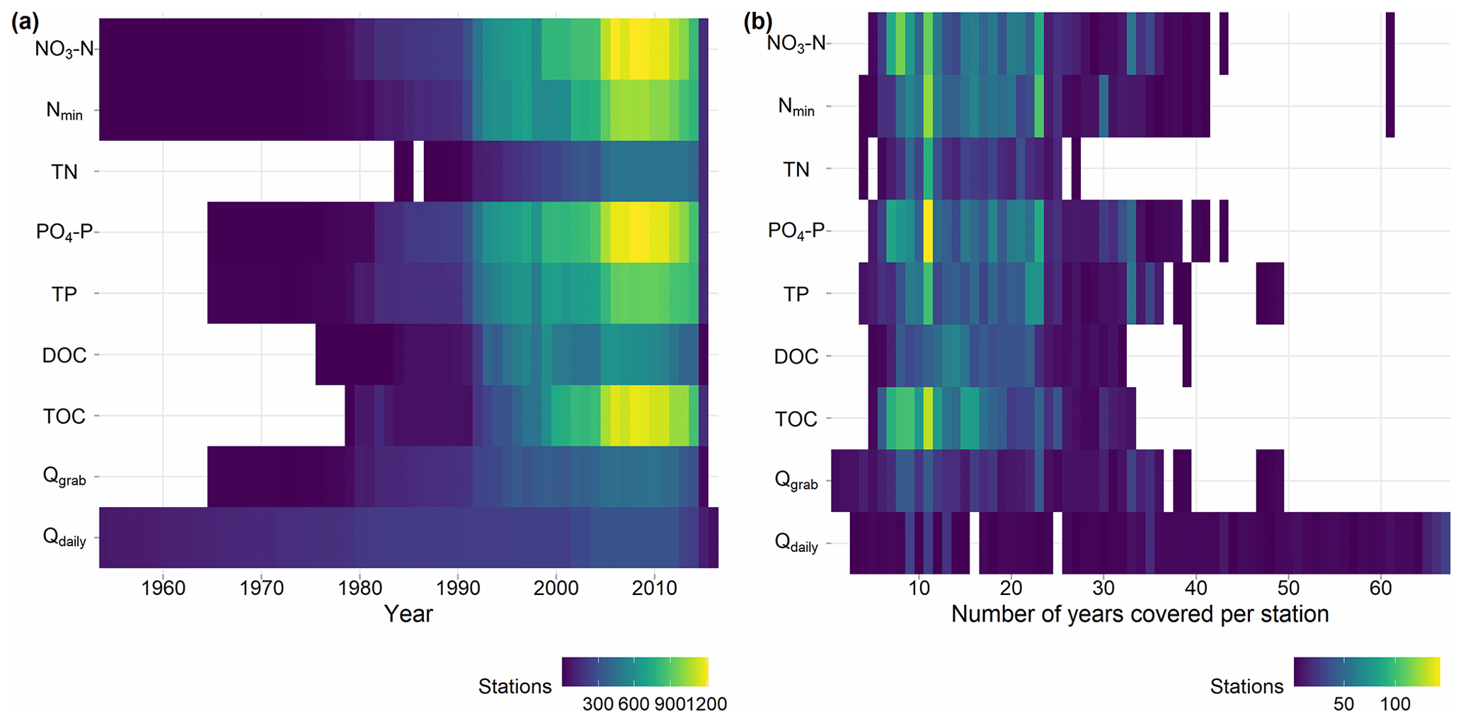
Figure 2Heat map of (a) the number of stations with available annual medians over time and per variable and (b) the number of years covered by each station. Qgrab refers to the median discharge (Q) from grab sample dates, and Qdaily refers to median Q from daily discharge (see Sect. 3.2.1 for details). For visualization purposes, in panel (a), station counts from 1954 are shown, omitting one concentration and a few Qdaily records before 1954; in panel (b), counts up to 67 years are shown, omitting three longer Qdaily records.
Table 2The number of stations with available data for the water quality compounds and discharge during grab sampling dates, the earliest and median start year of time series, the maximum and median time series length and covered years (i.e., years with available data), the median number of samples per stations and per station and year, and the number of outliers removed.
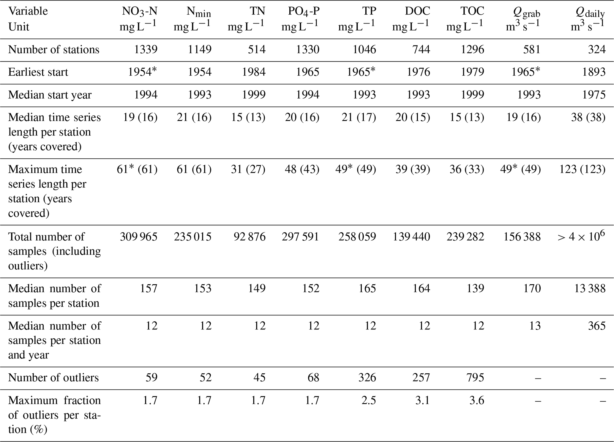
* Omitting one sample from 1900. The abbreviations used in the table are as follows: nitrate (NO3-N), mineral nitrogen (Nmin), total nitrogen (TN), phosphate (PO4-P), total phosphorus (TP), dissolved organic carbon (DOC), total organic carbon (TOC), the median discharge (Q) from grab sample dates (Qgrab), and the median Q from daily discharge (Qdaily).
3.1.2 Monthly median concentrations and mean fluxes for stations with high data availability
For the subset of stations with high data availability, a Weighted Regressions on Time, Discharge, and Season (WRTDS; Hirsch et al., 2010) analysis was applied using the “EGRET” R package (version 3.0.2; Hirsch and De Cicco, 2015). We refer to these stations as “WRTDS stations” for short. WRTDS represents long-term trends, seasonal components, and discharge-related variability in the water quality variables (Hirsch et al., 2010). The criteria for a WRTDS application were checked for each station and compound separately using the preprocessed data, as described in Sect. 2. The criteria were a time series of at least 20 years length, at least 150 samples of water quality, no data gaps larger than 20 % of the total time series length, and a complete time series of daily discharge (see also Sect. 3.2.2). The number of WRTDS stations varies between 44 for TN and 126 for PO4-P (Table 3), and the fraction of stations with high data availability varies between 4.9 % for TOC and 11.7 % for TP.
For WRTDS stations, we provide the monthly and annual median estimated water quality and observed quantity data in addition to the annual observed data (see above). More specifically, we provide monthly and annual median concentration and flow-normalized concentration as well as mean flux estimates from the WRTDS model output and median observed discharge (see Sect. 3.2.2) if data are available for at least 80 % of the respective time frame. The median R2 between WRTDS-modeled and observed concentrations varies between 0.44 for DOC and TOC and 0.75 for TN (Table 3); overall, 69.3 % of the catchment and compound combinations have a median R2 of at least 0.5. The median bias varies between −1.4 % for PO4-P (negative values indicate overestimation) and 0.2 % for NO3-N (positive values indicate underestimation); overall, 51 % of the catchments have a bias below 1 %, and 95 % of the catchments have a bias below 5 %. An overview of the availability of WRTDS stations and model performance is given in Table 3 and shown in Fig. A2, their locations are shown in Fig. 1a, and their performance is provided in the data repository.
Table 3The number of stations with high data availability (WRTDS stations) for each compound and the median coefficient of determination for WRTDS models.
The abbreviations used in the table are as follows: nitrate (NO3-N); mineral nitrogen (Nmin); total nitrogen (TN); phosphate (PO4-P); total phosphorus (TP); dissolved organic carbon (DOC); total organic carbon (TOC); and Weighted Regressions on Time, Discharge, and Season (WRTDS).
3.1.3 Monthly median concentrations over the time series
Next to annual and monthly time series, we provide long-term monthly medians over the complete time series of each station, enabling assessments of average seasonal variability. We also include the 25th and 75th percentiles to reflect the long-term variability in a given month. The provided data frame in QUADICA indicates the number of samples available for the corresponding month across the years, based on which representativeness can be assessed and quality criteria can be defined.
3.2 Water quantity time series
For about 43 % of the water quality stations (n=590), information on discharge is available (Fig. 1a) and is provided harmonized with the water quality data (i.e., at the annual and monthly resolution). The discharge information is a collection of data provided by the federal states along with the concentration data, either as daily discharge time series or for the times of grab sampling of water quality. Additionally, we integrated daily discharge data from 53 stations available from the Global Runoff Data Center (GRDC) to increase the number of stations with available discharge time series. We matched GRDC gauging stations to the existing water quality stations using a search radius of 500 m. For each match, we checked the consistency of river names and visually confirmed the locations. The corresponding GRDC station numbers are indicated in the metadata of the water quality and quantity data set (Musolff, 2020). For the original daily discharge data, the reader may refer to the regularly published and accessible data at the GRDC portal (https://portal.grdc.bafg.de, last access: 8 August 2022).
3.2.1 Annual median discharge
Annual median discharge is aggregated from available observed discharge data. For 324 water quality stations, a co-located Q station with a continuous daily Q record is available. However, the time series may include data gaps, and the time series of discharge and concentration data do not overlap at all for nine of the co-located discharge stations. For an additional 266 stations, Q data were only available at the time that the grab samples were taken. This resulted in a set of 581 stations for which Q data were available on the sampling dates of concentration data. We extracted annual median discharge from both continuous daily data (Qdaily) and dates when the water quality sample was taken (Qgrab, with a median of 13 values per year; Table 2) for the water quality stations. The density distribution of stations with available annual discharge over time is shown in Fig. 2a. Similar to the concentration data, the data availability is higher in more recent years, with a maximum of 449 stations in 2010. The number of years covered is, however, higher compared with water quality data for several stations (Fig. 2b). For stations with available daily discharge data, both annual median values of the daily data and the data from grab sample days were compared (Fig. A3). Our results suggest that annual median values from grab sample dates can be considered to be robust estimates of annual median discharge as they have a negligible bias (bias ) and low scatter around the 1:1 line (R2>0.99). The time series are shown in Appendix A (Fig. A1). The data set additionally provides the number of samples used to calculate the medians as a measure of robustness.
3.2.2 Monthly median discharge
Monthly median discharge is provided for WRTDS stations. To fill gaps in the daily discharge time series of the 45 stations required for WRTDS models (see Sect. 3.1.2), we used simulated discharge from the mesoscale hydrological model (mHM) (Kumar et al., 2013; Samaniego et al., 2010; Zink et al., 2017) if the regression coefficient (R2) between observed and simulated discharge for the station was greater than 0.6. Subsequently, modeled discharge was bias-corrected with piecewise linear regressions and used for gap filling (Ebeling et al., 2021b; Ehrhardt et al., 2021a). If modeled discharge was not available, small gaps (up to 7 days) were interpolated with fixed-interval smoothing using the “baytrends” R package (Murphy et al., 2019). Note that the gap-filled discharge time series are used for the WRTDS models only. This includes the monthly and annual discharge data provided with the WRTDS data tables (as described in Sect. 3.1.2).
3.2.3 Monthly median discharge over the time series
As for the water quality metrics (see Sect. 3.1.3), we provide long-term monthly median discharge and the 25th and 75th percentile over the whole time series, if available, for the station representing average discharge seasonality. The number of samples used for the calculation of medians is indicated as a measure of accuracy.
3.3 Meteorological time series
Meteorological time series are provided as spatial catchment averages at a monthly resolution. We used the daily gridded product of climate variables (precipitation and maximum, minimum, and average air temperature) from the “European Climate Assessment & Dataset” (ECA&D) project (E-OBS, v18.0e; Cornes et al., 2018). The advantage of a European data set is the coverage of transnational catchments, such as the Elbe or the Rhine. The data sets are available at a spatial resolution of 0.1∘ over the period from 1950 to 2018. The interpolation approach employed to create the gridded fields uses a stochastic technique based on Gaussian random field and involves several ground-based observation networks distributed across Europe (see Cornes et al., 2018, for more details). The daily fields of potential evapotranspiration are derived based on the method from Hargreaves and Samani (1985) at the same spatial resolution (0.1∘) using the daily (maximum, minimum, and average) air temperature data sets. We then calculated the spatial averages of daily climate variables (precipitation, air temperature, and potential evapotranspiration) for all water quality stations, considering the corresponding (upstream) catchment area. Monthly estimates of total precipitation and potential evapotranspiration as well as average air temperatures were subsequently calculated for each study basin.
3.4 Time series of net N input from diffuse sources
For the period from 1950 to 2015, we provide time series of catchment-scale N surplus (i.e., the net diffuse N input), which is the sum of N inputs minus the sum of N outputs from harvesting. At the catchment scale, the N surplus is the sum of N surplus from agricultural areas (Nagri; kg yr−1 ha−1) and nonagricultural areas (Nnonagri; kg yr−1 ha−1) normalized to the catchment area. For transboundary catchments with area outside of Germany, N surplus is normalized to the German part only. For nonagricultural areas, the N surplus is composed of atmospheric N deposition and biological N fixation. For agricultural areas, the N surplus includes additional N inputs (i.e., mineral fertilizer and manure applications) and N outputs from harvesting.
For agricultural land, the N surplus data stem from two data sets: one at the state level provided for the period from 1950 to 1998 (Behrendt et al., 2003, which builds on Bach and Frede, 1998, and Behrendt et al., 2000) and one at the county level provided for the period from 1995 to 2015 (Häußermann et al., 2019). To create a consistent long-term data set (1950–2015), we harmonized the county- and state-level data sets based on the overlapping years (1995–1998) and downscaled the state-level data to the county level for the period from 1950 to 1994. Specifically, we bias-corrected the state-level data of Behrendt et al. (2003) using proportions, as they commonly underestimated the values provided by Häußermann et al. (2019) for the period from 1995 to 1998. To downscale the bias-corrected state-level N surplus (1950–1994) to the county level, we used a linear regression between the county and state totals for the period from 1995 to 2015 (data from Häußermann et al., 2019). As data for city states (Berlin, Bremen, and Hamburg) are not provided in the state-level data set, we used the average value from 1995 to 1998 for the period from 1950 to 1994 under the assumption that the error is acceptable considering the small agricultural areas. The N surplus data comprise values for 5 of the 11 agricultural land classes in the CORINE (Coordination of Information on the Environment) Land Cover (CLC) inventory (EEA, 2016a): nonirrigated arable land, vineyards, fruit trees and berry plantations, pastures, and complex cultivation patterns. The data include N inputs from applications of fertilizers in mineral and organic forms, from seeds and planting material (county-level data only), from N deposition, and from biological N fixation as well as N outputs from harvested crops. To upscale agricultural N surplus from the county level to the catchment level, we used the fraction of agricultural area provided by CLC and a scaling factor. As CLC overestimates agricultural areas compared with the census data at the county level (Bach et al., 2006), we scaled the agricultural areas from CLC in each county by the mean ratio between the agricultural area from census data (Häußermann et al., 2019) and the CLC maps (years 2000, 2006, and 2012; median ratio of 1.24 across counties).
For nonagricultural land (CLC forest, water bodies, wetlands, and grassland classes) and the remaining agricultural land CLC classes not covered by the N surplus data described above (e.g., permanently irrigated land), we used the atmospheric N deposition data from the Meteorological Synthesizing Centre – West (MSC-W) of the European Monitoring and Evaluation Programme (EMEP; Simpson et al., 2012). The EMEP database uses a chemical transport model to generate a consistent gridded field of Europe-wide wet and dry as well as oxidized and reduced atmospheric N deposition (Simpson et al., 2012). The model assimilates varying levels of observational information on different atmospheric chemicals (e.g., Bartnicki and Benedictow, 2017; Bartnicki and Fagerli, 2006). The data were available for the period from 1980 to 1995 with 5-year time steps, which we linearly interpolated to obtain an annual time series, and with annual time steps for the period from 1995 to 2015. For the data before 1980, we assumed constant values from 1980 due to missing information. Deposition on urban sealed surfaces was neglected, as we assume that this component is collected by the sewer system and transported to the wastewater treatment plants. Thus, we assume it is not a diffuse N source but part of the point sources (Sect. 4.3). In contrast, deposition on urban grassland, like public parks, was considered. To account for the overestimated area of the five agricultural CLC classes in the agricultural N surplus data (see above), we added the corresponding missing fraction proportionally to the remaining land cover classes. We estimated terrestrial biological N fixation by plants for nonagricultural, vegetated areas using land-use-specific rates provided by Cleveland et al. (1999) and Van Meter et al. (2017).
The catchment-scale N surplus time series were calculated by intersecting the two N surplus components (Nagri and Nnonagri) with the respective land use and catchment area components. As the N surplus data were only available within Germany, data from transboundary catchments (e.g., the main stretch of the Elbe or Rhine rivers) need to be used cautiously, with higher uncertainty for catchments with a higher fraction of the catchment area outside of Germany (Sect. 4.3). Figure 3 shows the resulting N input time series of all catchments. The majority of N input stems from agriculture, with a median of 64 % of the total catchment N surplus stemming from Nagri across all catchments (averages between 1950 and 2015). The agricultural N surplus (Nagri) and its fraction per catchment were highest during the 1980s, with a median across catchments of 52 kg ha−1 yr−1 and 76 % (average between 1980 and 1989), respectively. The highest mean agricultural N surplus and annual fraction across all catchments were reached in 1988, with respective values of 60.7 kg ha−1 yr−1 and 74 %, although these values were already above 50 kg ha−1 yr−1 and 70 % from 1976 to 1989. For the total N surplus, the mean annual values across catchments were above 70 kg ha−1 yr−1 during the same period (1976–1989), although values were above 50 kg ha−1 yr−1 from 1969, and the maximum of 76.7 kg ha−1 yr−1 occurred in 1980.
Figure 3Time series of annual N surplus for all catchments for the different N surplus components: N surplus for nonagricultural areas (a), N surplus for agricultural areas (b), and total N surplus for both nonagricultural and agricultural areas (c). Box plots represent the distribution of the annual N surplus as averages of the German catchment area across all catchments showing summary statistics (median, quartiles, and quartiles ±1.5 times the interquartile range) and individual points outside these ranges. The black lines represent the mean annual values for each N surplus component across the catchments.
The provided catchment attributes characterize the catchments in terms of topography, land cover, nutrient sources, lithology and soils, and hydroclimate. The attributes were chosen with a focus on macronutrient sources and transport in line with the data set. Figure 4 shows the spatial distribution of a set of selected catchment attributes. All attributes, their variable names, original data sources, and methods are listed in Appendix B (Table B1) and the data repository (Ebeling et al., 2022a). This repository of catchment attributes is a composite of attributes from two existing repositories (Ebeling and Dupas, 2021; Ebeling, 2021).
4.1 Location and topography
Catchment size was calculated from the delineated catchment boundaries described in Sect. 2. Catchment size ranges from 0.9 to 123 012 km2, with a median of 171.2 km2 , a 25th percentile of 53.6, and a 75th percentile of 634.4 km2. Additionally, the fraction of the catchment area lying within German borders was calculated (f_AreaGer). Mean and median catchment elevation and topographic slope were extracted from the DEM with a 100 m resolution (see also Sect. 2; EEA, 2013). A 100 m grid of the topographic wetness index (TWI) was calculated from the DEM by relating the upstream area (from flow accumulation) to the local slope at each grid cell, following Beven and Kirkby (1979). For each catchment, we extracted mean, median, and 90th percentile TWI values. The 90th percentile has been shown to be a proxy for the abundance of riparian wetlands in a catchment (Musolff et al., 2018). Drainage density, defined as the length of surface waters per area, closely relates to topography. Drainage density was calculated and provided in two ways: as the catchment average of the gridded drainage density (cell size 0.012∘) provided in the Hydrologischer Atlas Deutschland (BMU, 2000) and as the river length from EU-Hydro River Network Database (EEA, 2019) within the catchment divided by its area. For the latter, the level of detail was too coarse to yield plausible values for all catchments, which is why values are missing for 27 of the smaller catchments. However, the EU-Hydro River Network Database provides further stream attributes such as the Strahler order.

Figure 4Maps of selected catchment attributes. Each dot represents one station, and the color represents the attribute of the corresponding catchment. Colors are according to the quartiles of the data distribution of each attribute. The attributes shown are as follows: dem.mean – average elevation [m], twi.90p – 90th percentile of the topographic wetness index [–], P_mm – mean annual precipitation [mm yr−1], AI – aridity index [–], T_mean – mean air temperature [∘C], specQobs – specific annual discharge [mm yr−1], f_sedim – fraction of sedimentary aquifer [–], f_sand – fraction of sandy soils [–], pdens – population density [inhabitants km−2], het_v – vertical concentration heterogeneity [–], Nsurp80_15 – mean N surplus from 1980 to 2015 [kg N ha−1 yr−1], and soilP.mean – phosphorus content in topsoil [mg kg−1]. For more details on the attributes, the reader is referred to the text in Sect. 4 and Table B1.
4.2 Land cover and population density
The fractions of land cover classes were calculated from the level 1 classification of the CLC data set for 2012 (artificial, agricultural, forested land, wetland, and surface water cover) (EEA, 2016a). For a finer distinction within these overall classes, fractions of land cover classes were additionally calculated from level 2 data. Note that there can be an overestimation of agricultural areas from these CLC land cover classes when compared with census data as described by Bach et al. (2006) and considered for N surplus time series (Sect. 3.4). Nevertheless, we expect that the relative distribution of agricultural fractions among the catchments is well captured. The mean catchment population density was calculated from the Gridded Population of the World data set (CIESIN, 2017) for 2010.
4.3 Nutrient sources
The input from point sources is calculated as the sum of the N and P load from wastewater treatment plants (WWTPs) with more than 2000 population equivalents (PEs) from the database of the European Environment Agency (EEA, 2017) and data collected from 13 German federal states covering smaller WWTPs (PE <2000) within Germany (Büttner, 2020). One PE is defined as the organic biodegradable load having a 5-day biochemical oxygen demand (BOD5) of 60 g of oxygen per day (EC, 1991a). As a second data source, we calculated catchment averages of the European domestic waste emissions database (Vigiak et al., 2019, 2020) for N, P, and BOD5 inputs from point sources. The average N, P, and BOD5 input per person was estimated using the point source input divided by the number of inhabitants according to the population density. The advantage of these European data is the consistency for an extended transnational data set – for example, it is available for German and French catchments (Ebeling and Dupas, 2021).
The net N input from diffuse sources was determined as temporal averages of diffuse N surplus time series (Sect. 3.4) for different periods, representing the main sampling period with historic inputs (1980–2015) and the current period (2000–2015). We also calculated averages for the periods before (1971–1990) and after (1991–2015) the EU 91/676/EEC Nitrates Directive (EC, 1991b) as well as the difference between them, which was used as a characteristic of net input change. Note that the N surplus data used only cover Germany, but catchments can be transnational. The uncertainty increases for larger areas outside of Germany, for which f_AreaGer can be used as a measure. To estimate source apportionment between point and diffuse N sources, we calculated the fraction of catchment point source N loads (N_WW_frac) from total catchment N input as the sum of catchment point source N loads from domestic waste emissions (N_T_YKM2) and N surplus (here using Nsurp80_15 for the period from 1980 to 2015) on average:
We defined horizontal and vertical source heterogeneity in catchments to quantify the spatial distribution of diffuse nutrient sources with a focus on NO3-N (Ebeling et al., 2021a). The horizontal source heterogeneity describes the distribution of agricultural land use in a catchment in relation to the stream network. We used the horizontal flow distance of the 100 m DEM (EEA, 2013; Sect. 2) to the EU-Hydro River Network Database (EEA, 2019) and a highly resolved land use map of 2015 provided by Pflugmacher et al. (2018). We divided the grid into classes of flow distance to stream with 400 m steps. Subsequently, we fitted a linear regression to the share of agricultural source areas in each of the distance classes and the mean distance of the range of each distance class (i.e., 200 m for the class 0–400 m) weighted by the abundance of that specific class. The slope of the resulting linear model het_h characterizes if agricultural source areas tend to be located close to the stream network (het_h <0), equally distributed (het_h =0), or located far away from the stream network (het_h >0). For more details, the reader is referred to Ebeling et al. (2021a). The vertical source heterogeneity het_v is the ratio of the shallow to deep NO3-N concentrations. Shallow NO3-N concentrations are estimated on a 1 km grid by Knoll et al. (2020) using a 10-year average of N surplus and average groundwater recharge. This can be seen as a potential leachate concentration, as denitrification in the soil's root zone and horizontal transport are not accounted for. The deep NO3-N concentrations are estimated on the same grid using a random forest model that is trained on observed concentrations in groundwater (Knoll et al., 2020). The ratio of both was averaged across the catchment to yield het_v reported here. A ratio of 1 describes a catchment that has a vertical homogeneity in NO3-N concentrations, whereas a ratio above 1 describes stronger vertical concentration gradients.
4.4 Lithology and hydrogeology
To characterize the lithological and the hydrogeological settings of the catchments, we used the International Hydrogeological Map of Europe 1:1 500 000 (BGR and UNESCO, 2014). For the lithological settings, we derived the fraction of area covered by calcareous rocks, calcareous rocks and sediments, magmatic rocks, metamorphic rocks, siliciclastic rocks, siliciclastic rocks and sediments, and sediments (based on level 4 lithology data). Additionally, we determined the fractions of the more aggregated lithological classes (from level 5 lithology), i.e., consolidated, partly consolidated, and unconsolidated rocks. Furthermore, we quantified the areal fraction of aquifer type in the catchment, differentiating between porous aquifers, fissured hard-rock aquifers (including karst), and locally aquiferous or non-aquiferous rocks. Finally, we extracted the catchment median estimate of depth to bedrock from the global map from Shangguan et al. (2017).
4.5 Soil properties
We calculated the fraction of the catchment covered with hydromorphic soils (Stagnosols, semiterrestrial, semi-subhydric, subhydric, and peat soils) from the German soil map (1:250 000; BGR, 2018). As this data source only covers Germany, data might not be reliable for transboundary catchments (see also Sect. 4.3). We also calculated the average fraction of sand, silt, and clay averaged across the soil horizons of the top 1 m based on the Harmonized World Soil Database (HWSD; v1.2) available as a 30 arcsec raster database (FAO/IIASA/ISRIC/ISSCAS/JRC, 2012). We first estimated vertically weighted soil textural properties from the original HWSD data provided for two soil layers (upper 30 and 30–100 cm). Next, we calculated the areal averages of respective properties considering the boundary (polygon) of each study catchment.
We estimated the porosity of soil profiles (thetaS) based on the pedotransfer function of Zacharias and Wessolek (2007) and the root zone plant-available water content (WaterRoots), which reflects the difference in water content between the field capacity and permanent wilting point. The field capacity is calculated based on a flux-based estimation approach proposed by Twarakavi et al. (2009) corresponding to a minimum drainage flux of 1 mm d−1. The estimate of the permanent wilting point is derived using the van Genuchten (1980) model of the matric potential at −1500 kPa and the corresponding model parameters calculated from pedotransfer functions of Zacharias and Wessolek (2007). Similar to soil textural properties, for each of these soil hydraulic parameters (porosity, field capacity, and permanent wilting point), we calculated areal averages of the vertically weighted estimates for the upper 1 m of the soil profile for each study catchment. More details on this method of using pedotransfer functions and subsequent aggregations can be found in Livneh et al. (2015). Furthermore, we estimated average catchment soil chemistry of the topsoil (first 20 cm) for the year 2009 from the European soil chemistry map, which is based on the LUCAS (Land Use and Cover Area frame Survey) database (Ballabio et al., 2019). For this, we calculated the mean C N ratio, nitrogen content, and phosphorus content from the maps for each catchment.
4.6 Hydroclimatic characteristics
Long-term average hydroclimatic characteristics were derived from the meteorological (Sect. 3.3) and discharge time series. All climatic characteristics were calculated for a period of 30 years from 1986 to 2015 based on the E-OBS data set from the ECA&D project (v18.0e; Cornes et al., 2018). First, we provide mean annual precipitation, mean annual potential evapotranspiration, mean annual air temperature, and the aridity index as the ratio between potential evapotranspiration and precipitation. The variability in precipitation is further characterized by the mean precipitation frequency and depth (Botter et al., 2013) as well as by two seasonality indices, i.e., the ratio between summer (June–August) and winter (December–February) precipitation (P_SIsw) and the average difference between average daily precipitation within each month and within a year (P_SI).
The hydrologic properties were characterized from stations with observed daily discharge data (Sect. 3.2) for different time periods according to the available data and study purposes of the original data sets. For current properties, daily discharge data from November 1999 (hydrological year 2000) were used for calculations (309 stations). Additionally, the hydrologic characteristics calculated from daily discharge data starting in 1986 are provided (319 stations), which are possibly more relevant for studies with a long-term perspective. If there were only data before 1986, we used the available time period (four stations). The actual starting and ending dates of the time series finally used for calculations are provided to inform the user of the exact time periods (StartQobs and EndQobs or Q_StartDate and Q_EndDate, respectively, refer to Table B1). Provided average characteristics include mean, median, median summer (May–October), median winter (November–April), and specific discharge. For the variability in discharge, we provide the coefficient of variation, the base flow index (according to WMO, 2008), and the flashiness index based on flow percentiles (ratio of the 5th to the 95th percentile) as well as discharge seasonality in terms of the ratio between summer and winter median discharge and the runoff coefficient (discharging fraction of precipitation).
The presented data set has several limitations. More than half of the stations do not a have co-located gauging station and the ones that do are not homogeneously distributed across Germany. Existing concentration time series would benefit from available discharge data, as this allows the characterization of concentration-discharge relationships as well as the estimation of daily concentration, flow-normalized concentration and flux data for stations with high data availability using the WRTDS method. Generally, modeled discharge from hydrological models such as mHM (Sect. 3.2.2) or estimated discharge using other (mechanistic or statistical modeling) techniques could serve to extend the data set of joint water quality and water quantity and overcome missing station matches or data gaps. Other limitations are linked to data policies by federal state authorities, which sometimes do not permit publication of raw quality and quantity data. However, we aimed to make a virtue of necessity by providing aggregated data and further ready-to-use metrics of water quality and quantity (e.g., annual median concentrations and monthly median concentrations over the whole time series). Attributes derived from exclusively national data sets, such as N surplus, underlie higher uncertainties in transboundary catchments, as data outside Germany are either not available or not consistent. Additionally, there is uncertainty in the attributes, stemming from the inherent uncertainties in the data sets and the catchment boundaries. However, the provided description and references of the methods and the underlying data sources should enable users to evaluate the reliability of each descriptor in the data set and exclude stations from the analyses if necessary. This also leaves room for further improvements and extensions when new data and knowledge become available. Besides a higher number of water quality stations, longer time series and more co-located discharge data, it would be especially interesting to add time series of nutrient inputs from point sources and from diffuse P sources, as well as information on tile drainage locations to the catchment attributes. For a better linkage of chemical water quality with ecological research questions, biological water quality variables such as chlorophyll-a concentrations would be highly valuable as well.
The QUADICA data set presented here is freely available from two online repositories. The water quality and water quantity data described in this paper as well as the time series of meteorological and diffuse nitrogen input can be accessed at https://doi.org/10.4211/hs.0ec5f43e43c349ff818a8d57699c0fe1 (Ebeling et al., 2022b). The catchment data, including the catchment attributes, boundaries, and stations, have been published at https://doi.org/10.4211/hs.88254bd930d1466c85992a7dea6947a4 (Ebeling et al., 2022a). Due to license agreements, the raw concentration and raw discharge data provided by the German federal states cannot made public, but they have been deposited in an institutional repository (Musolff et al., 2020). The metadata of the data and stations, however, are available from https://doi.org/10.4211/hs.a42addcbd59a466a9aa56472dfef8721 (Musolff, 2020).
In this study, we provide a comprehensive homogenized data set with a large spatial and temporal coverage of both water quality and quantity observations along with catchment attributes. Specifically, the data set includes time series of water quality, co-located discharge, hydroclimatic data, and diffuse nitrogen inputs as well as catchment boundaries and more than 100 catchment attributes for 1386 German catchments. The presented QUADICA (water QUAlity, DIscharge and Catchment Attributes for large-sample studies in Germany) data set offers the opportunity to identify spatial and temporal patterns of water quality along with water quantity. This allows one to formulate and test hypotheses on underlying processes by linking observed responses to the driving forces and catchment attributes. QUADICA also opens up opportunities to calibrate and validate water and solute transport models at the single- and multiple-catchment scales as well as at the national scale. Consequently, the data set has the potential to advance our understanding of water quality processes across scales. More specifically, the data can be used to examine various spatiotemporal water quality patterns such as average concentrations, trends, and average seasonality. For stations with high data availability, analyses can be extended to trajectories of seasonality, flow-normalized concentrations, and mass fluxes. The patterns can be investigated for the three different macronutrients, nitrogen, phosphorus, and organic carbon; their species; and for nutrient ratios. In addition, interactions between the nutrients and their spatiotemporal patterns can be assessed. In the context of comparative large-sample hydrology (e.g., Gupta et al., 2014), the spatiotemporal water quality patterns can be linked to catchment attributes to identify underlying processes. This can, for example, support quantification of the impact of human disturbances on nutrient cycles and their interactions with natural controls. Some studies have recently investigated spatiotemporal patterns and underlying controls in large-sample approaches using parts of the provided data set. For example, Ebeling et al. (2021a) assessed average nutrient concentrations and export dynamics, Ebeling et al. (2021b) evaluated long-term trajectories of nitrate seasonality, Ehrhardt et al. (2021b) quantified nitrogen legacies using nitrogen input and export time series, and Yang et al. (2021) modeled the impact of phosphorus inputs on stream network algae growth. These assessments and the derived hypotheses can be further explored and extended with the provided data to increase our knowledge on catchment functioning.
Furthermore, the provided data can be merged with other water quality and quantity data sets – for example, to enable assessments across transnational scales and an even larger variability in catchment attributes. Here, we hope to stimulate other researchers or environmental authorities to provide similar data sets of joint water quality and quantity data to make the wealth of spatiotemporal water quality data available, including long-term data that have been collected during research projects and regular monitoring activities, such as for the 2000/60/EC EU Water Framework Directive (EC, 2000). Therefore, we call for joint efforts to further increase opportunities for catchment-scale water quality assessments and modeling activities on regional, transnational, and even continental scales.

Figure A1Time series of annual median concentrations and discharge observed at the 1386 water quality stations during grab sampling, as shown in Table 1 and Fig. 1 and described in Sect. 3.1. Note that, for visualization purposes, values before 1954 and values >40 mg L−1 for N species (i.e., five NO3-N, seven Nmin, and zero TN values) are not shown.

Figure A2Distribution of the performance of WRTDS models by compound based on the coefficient of determination R2 (a) and bias (b). Boxes highlight the median and quartiles of each distribution, and points display the performance values of single catchments. Note that, for visualization purposes, one bias value >0.4 is not shown for TOC.

Figure A3Comparison of annual medians from continuous daily discharge (Qdaily) and discharge at the dates grab samples were taken (Qgrab). Colors represent different catchments.
Table B1Catchment attributes, associated methods, and original data sources used for calculating the attributes (Ebeling et al., 2022a). This collection of catchment attributes is merged and adapted from existing repositories (Ebeling, 2021; Ebeling and Dupas, 2021) and the related publications (Ebeling et al., 2021a, b). For more details, the reader is referred to Sect. 4.
PE carried out the study, processed and curated the data, and created the figures and tables. PE, AM, and RK conceptualized and designed the study; AM and SA provided the initial ideas for the study and obtained funding. Several authors contributed to the data collection and processing: RK provided the gridded meteorological time series, simulated discharge data, and atmospheric deposition data; MW provided time series of N surplus data for the catchments; and OB collected the point source data for Germany. PE produced the original draft of the paper with contributions from AM and RK. All authors contributed to reviewing and editing the manuscript.
The contact author has declared that none of the authors has any competing interests.
Publisher's note: Copernicus Publications remains neutral with regard to jurisdictional claims in published maps and institutional affiliations.
The authors gratefully thank all data collectors, processors, and providers, including the federal state environmental agencies and all contributors to this data set. We are especially grateful to Thomas Grau, Teresa Nitz, Joni Dehaspe, Stefanie Breese, and Sophie Ehrhardt for their contributions to data processing. The authors wish to thank the two anonymous reviewers for their valuable comments. Moreover, we gratefully acknowledge Martin Bach and Uwe Häußermann (Justus-Liebig-Universität Giessen) for the provision of the two data sets on the agricultural N surplus data for Germany. We acknowledge the E-OBS data set from the EU FP6 project UERRA (http://www.uerra.eu, last access: 8 August 2022) and the Copernicus Climate Change Service, and the data providers for the ECA&D project (https://www.ecad.eu, last access: 8 August 2022). The authors additionally acknowledge several organizations responsible for the data products used here, including the BfG, BGR, SGD, EEA, FAO, IIASA, ISRIC, ISSCAS, and JRC.
This research has been supported by the Deutsche Forschungsgemeinschaft (grant no. 392886738).
This paper was edited by David Carlson and reviewed by two anonymous referees.
Addor, N., Newman, A. J., Mizukami, N., and Clark, M. P.: The CAMELS data set: catchment attributes and meteorology for large-sample studies, Hydrol. Earth Syst. Sci., 21, 5293–5313, https://doi.org/10.5194/hess-21-5293-2017, 2017.
Addor, N., Do, H. X., Alvarez-Garreton, C., Coxon, G., Fowler, K., and Mendoza, P. A.: Large-sample hydrology: recent progress, guidelines for new datasets and grand challenges, Hydrolog. Sci. J., 65, 712–725, https://doi.org/10.1080/02626667.2019.1683182, 2020.
Alvarez-Garreton, C., Mendoza, P. A., Boisier, J. P., Addor, N., Galleguillos, M., Zambrano-Bigiarini, M., Lara, A., Puelma, C., Cortes, G., Garreaud, R., McPhee, J., and Ayala, A.: The CAMELS-CL dataset: catchment attributes and meteorology for large sample studies – Chile dataset, Hydrol. Earth Syst. Sci., 22, 5817–5846, https://doi.org/10.5194/hess-22-5817-2018, 2018.
Bach, M. and Frede, H.-G.: Agricultural nitrogen, phosphorus and potassium balances in Germany – Methodology and trends 1970 to 1995, Z. Pflanz. Bodenkunde, 161, 385–393, https://doi.org/10.1002/jpln.1998.3581610406, 1998.
Bach, M., Breuer, L., Frede, H. G., Huisman, J. A., Otte, A., and Waldhardt, R.: Accuracy and congruency of three different digital land-use maps, Landscape Urban Plan., 78, 289–299, https://doi.org/10.1016/j.landurbplan.2005.09.004, 2006.
Ballabio, C., Lugato, E., Fernández-Ugalde, O., Orgiazzi, A., Jones, A., Borrelli, P., Montanarella, L., and Panagos, P.: Mapping LUCAS topsoil chemical properties at European scale using Gaussian process regression, Geoderma, 355, 113912, https://doi.org/10.1016/j.geoderma.2019.113912, 2019.
Bartnicki, J. and Benedictow, A.: Atmospheric Deposition of Nitrogen to OSPAR Convention waters in the period 1995–2014, EMEP/MSC-W Technical Report, 1/2007, Meteorological Synthesizing Centre-West (MSC-W), Norwegian Meteorological Institute, Oslo, https://emep.int/publ/reports/2017/MSCW_technical_1_2017.pdf (last access: 11 August 2022), 2017.
Bartnicki, J. and Fagerli, H.: Atmospheric Nitrogen in the OSPAR Convention Area in the Period 1990–2004. Summary Report for the OSPAR Convention, EMEP/MSC-W Technical Report, 4/2006, Meteorological Synthesizing Centre-West (MSC-W) of EMEP, Oslo, https://www.ospar.org/documents?v=7064 (last access: 12 August 2022), 2006.
Basu, N. B., Destouni, G., Jawitz, J. W., Thompson, S. E., Loukinova, N. V., Darracq, A., Zanardo, S., Yaeger, M., Sivapalan, M., Rinaldo, A., and Rao, P. S. C.: Nutrient loads exported from managed catchments reveal emergent biogeochemical stationarity, Geophys. Res. Lett., 37, L23404, https://doi.org/10.1029/2010gl045168, 2010.
Behrendt, H., Huber, P., Opitz, D., Schmoll, O., Scholz, G., and Uebe, R.: Nutrient emissions into river basins of Germany, UBA-Texte, 75/99, https://www.umweltbundesamt.de/en/publikationen/naehrstoffbilanzierung-flussgebiete-deutschlands (last access: 8 August 2022), 1999.
Behrendt, H., Huber, P., Opitz, D., Schmoll, O., Scholz, G., and Uebe, R.: Nutrient emissions into river basins of Germany, UBA-Texte, 23/00, https://www.umweltbundesamt.de/en/publikationen/nutrient-emissions-into-river-basins-of-germany (last access: 9 August 2022), 2000.
Behrendt, H., Bach, M., Kunkel, R., Opitz, D., Pagenkopf, W.-G., Scholz, G., and Wendland, F.: Nutrient Emissions into River Basins of Germany on the Basis of a Harmonized Procedure UBA-Texte, 82/03, https://www.umweltbundesamt.de/en/publikationen/nutrient-emissions-into-river-basins-of-germany-on (last access: 9 August 2022), 2003.
Beven, K. J. and Kirkby, M. J.: A physically based, variable contributing area model of basin hydrology/Un modèle à base physique de zone d'appel variable de l'hydrologie du bassin versant, Hydrol. Sci. B., 24, 43–69, https://doi.org/10.1080/02626667909491834, 1979.
BGR: Bodenübersichtskarte der Bundesrepublik Deutschland 1:250.000 (BUEK250). Soil map of Germany 1:250,000, Federal Institute for Geosciences and Natural Resources (BGR) [data set], https://produktcenter.bgr.de/terraCatalog/Start.do (last access: 9 August 2022), 2018.
BGR and UNESCO (Eds.): International Hydrogeological Map of Europe 1:1 500 000 (IHME1500). Digital map data v1.1. [data set], http://www.bgr.bund.de/ihme1500/ (last access: 9 August 2022), 2014.
BMU (Bundesministerium Für Umwelt) (Ed.): Hydrologischer Atlas von Deutschland, Datenquelle: Hydrologischer Atlas von Deutschland/BfG, 2000, Bonn, Berlin, https://geoportal.bafg.de/mapapps/resources/apps/HAD/index.html (last access: 9 August 2022), 2000.
Botter, G., Basso, S., Rodriguez-Iturbe, I., and Rinaldo, A.: Resilience of river flow regimes, P. Natl. Acad. Sci. USA, 110, 12925–12930, https://doi.org/10.1073/pnas.1311920110, 2013.
Büttner, O.: DE-WWTP – data collection of wastewater treatment plants of Germany (status 2015, metadata), HydroShare [data set], https://doi.org/10.4211/hs.712c1df62aca4ef29688242eeab7940c, 2020.
Center for International Earth Science Information Network – CIESIN – Columbia University: Gridded Population of the World, Version 4 (GPWv4): Population Density, Revision 10, NASA Socioeconomic Data and Applications Center (SEDAC) [data set], https://doi.org/10.7927/H4DZ068D, 2017.
Chagas, V. B. P., Chaffe, P. L. B., Addor, N., Fan, F. M., Fleischmann, A. S., Paiva, R. C. D., and Siqueira, V. A.: CAMELS-BR: hydrometeorological time series and landscape attributes for 897 catchments in Brazil, Earth Syst. Sci. Data, 12, 2075–2096, https://doi.org/10.5194/essd-12-2075-2020, 2020.
Chen, D., Shen, H., Hu, M., Wang, J., Zhang, Y., and Dahlgren, R. A.: Chapter Five – Legacy Nutrient Dynamics at the Watershed Scale: Principles, Modeling, and Implications, in: Advances in Agronomy, edited by: Sparks, D. L., Academic Press, 237–313, https://doi.org/10.1016/bs.agron.2018.01.005, 2018.
Cleveland, C. C., Townsend, A. R., Schimel, D. S., Fisher, H., Howarth, R. W., Hedin, L. O., Perakis, S. S., Latty, E. F., Von Fischer, J. C., Elseroad, A., and Wasson, M. F.: Global patterns of terrestrial biological nitrogen (N2) fixation in natural ecosystems, Global Biogeochem. Cy., 13, 623–645, https://doi.org/10.1029/1999GB900014, 1999.
Cornes, R. C., van der Schrier, G., van den Besselaar, E. J. M., and Jones, P. D.: An Ensemble Version of the E-OBS Temperature and Precipitation Data Sets, J. Geophys. Res.-Atmos., 123, 9391–9409, https://doi.org/10.1029/2017jd028200, 2018.
Coxon, G., Addor, N., Bloomfield, J. P., Freer, J., Fry, M., Hannaford, J., Howden, N. J. K., Lane, R., Lewis, M., Robinson, E. L., Wagener, T., and Woods, R.: CAMELS-GB: hydrometeorological time series and landscape attributes for 671 catchments in Great Britain, Earth Syst. Sci. Data, 12, 2459–2483, https://doi.org/10.5194/essd-12-2459-2020, 2020.
De Jager, A. and Vogt, J.: Rivers and Catchments of Europe – Catchment Characterisation Model (CCM) (2.1), European Commission, Joint Research Centre (JRC) [data set], http://data.europa.eu/89h/fe1878e8-7541-4c66-8453-afdae7469221 (last access: 9 August 2022), 2007.
Do, H. X., Westra, S., and Leonard, M.: A global-scale investigation of trends in annual maximum streamflow, J. Hydrol., 552, 28–43, https://doi.org/10.1016/j.jhydrol.2017.06.015, 2017.
Ebeling, P.: CCDB – catchment characteristics data base Germany, HydroShare [data set], https://doi.org/10.4211/hs.0fc1b5b1be4a475aacfd9545e72e6839, 2021.
Ebeling, P. and Dupas, R.: CCDB – catchment characteristics data base France and Germany, HydroShare [data set], https://doi.org/10.4211/hs.c7d4df3ba74647f0aa83ae92be2e294b, 2021.
Ebeling, P., Kumar, R., Weber, M., Knoll, L., Fleckenstein, J. H., and Musolff, A.: Archetypes and Controls of Riverine Nutrient Export Across German Catchments, Water Resour. Res., 57, e2020WR028134, https://doi.org/10.1029/2020WR028134, 2021a.
Ebeling, P., Dupas, R., Abbott, B., Kumar, R., Ehrhardt, S., Fleckenstein, J. H., and Musolff, A.: Long-Term Nitrate Trajectories Vary by Season in Western European Catchments, Global Biogeochem. Cy., 35, e2021GB007050, https://doi.org/10.1029/2021GB007050, 2021b.
Ebeling, P., Kumar, R., and Musolff, A.: CCDB – catchment characteristics data base Germany, HydroShare [data set], https://doi.org/10.4211/hs.88254bd930d1466c85992a7dea6947a4, 2022a.
Ebeling, P., Kumar, R., Weber, M., and Musolff, A.: QUADICA – water quality, discharge and catchment attributes for large-sample studies in Germany, HydroShare [data set], https://doi.org/10.4211/hs.0ec5f43e43c349ff818a8d57699c0fe1, 2022b.
EC: Council Directive 91/271/EEC of 21 May 1991 concerning urban waste water treatment, Official Journal of the European Communities, http://data.europa.eu/eli/dir/1991/271/oj (last access: 9 August 2022), 1991a.
EC: Council Directive 91/676/EEC of 12 December 1991 concerning the protection of waters against pollution caused by nitrates from agricultural sources, Official Journal of the European Communities, http://data.europa.eu/eli/dir/1991/676/oj (last access: 9 August 2022), 1991b.
EC: Directive 2000/60/EC of the European Parliament and of the Council of 23 October 2000 establishing a framework for Community action in the field of water policy, Official Journal of the European Communities, L 327, 1–73, http://data.europa.eu/eli/dir/2000/60/oj (last access: 9 August 2022), 2000.
EEA: DEM over Europe from the GMES RDA project (EU-DEM, resolution 25 m) – version 1, European Environment Agency [data set], https://www.eea.europa.eu/data-and-maps/data/eu-dem (last access: 9 August 2022), 2013.
EEA: CORINE Land Cover 2012 v18.5, European Environment Agency [data set], https://land.copernicus.eu/pan-european/corine-land-cover/clc-2012 (last access: 11 August 2022), 2016.
EEA: Waterbase – UWWTD: Urban Waste Water Treatment Directive – reported data (v5), European Environment Agency [data set], https://www.eea.europa.eu/data-and-maps/data/waterbase-uwwtd-urban-waste-water-treatment-directive-5 (last access: 9 August 2022), 2017.
EEA: EU-Hydro – River Network Database (v1), European Environment Agency [data set], https://land.copernicus.eu/imagery-in-situ/eu-hydro/eu-hydro-river-network-database (last access: 9 August 2022), 2019.
EEA: Waterbase – Water Quality ICM, European Environment Agency [data set], https://www.eea.europa.eu/data-and-maps/data/waterbase-water-quality-icm-2 (last access: 9 August 2022), 2020.
Ehrhardt, S., Ebeling, P., and Dupas, R.: Exported french water quality and quantity data, HydroShare [data set], https://doi.org/10.4211/hs.d8c43e1e8a5a4872bc0b75a45f350f7a, 2021a.
Ehrhardt, S., Ebeling, P., Dupas, R., Kumar, R., Fleckenstein, J. H., and Musolff, A.: Nitrate Transport and Retention in Western European Catchments Are Shaped by Hydroclimate and Subsurface Properties, Water Resour. Res., 57, e2020WR029469, https://doi.org/10.1029/2020WR029469, 2021b.
FAO/IIASA/ISRIC/ISSCAS/JRC: Harmonized World Soil Database (version 1.2), FAO, Rome, Italy and IIASA, Laxenburg, Austria [data set], https://webarchive.iiasa.ac.at/Research/LUC/External-World-soil-database/HTML/ (last access: 11 August 2022), 2012.
Fowler, K. J. A., Acharya, S. C., Addor, N., Chou, C., and Peel, M. C.: CAMELS-AUS: hydrometeorological time series and landscape attributes for 222 catchments in Australia, Earth Syst. Sci. Data, 13, 3847–3867, https://doi.org/10.5194/essd-13-3847-2021, 2021.
Gnann, S. J., Howden, N. J. K., and Woods, R. A.: Hydrological signatures describing the translation of climate seasonality into streamflow seasonality, Hydrol. Earth Syst. Sci., 24, 561–580, https://doi.org/10.5194/hess-24-561-2020, 2020.
Godsey, S. E., Kirchner, J. W., and Clow, D. W.: Concentration-discharge relationships reflect chemostatic characteristics of US catchments, Hydrol. Process., 23, 1844–1864, https://doi.org/10.1002/hyp.7315, 2009.
Godsey, S. E., Hartmann, J., and Kirchner, J. W.: Catchment chemostasis revisited: Water quality responds differently to variations in weather and climate, Hydrol. Process., 33, 3056–3069, https://doi.org/10.1002/hyp.13554, 2019.
Gupta, H. V., Perrin, C., Blöschl, G., Montanari, A., Kumar, R., Clark, M., and Andréassian, V.: Large-sample hydrology: a need to balance depth with breadth, Hydrol. Earth Syst. Sci., 18, 463–477, https://doi.org/10.5194/hess-18-463-2014, 2014.
Hargreaves, G. H. and Samani, Z. A.: Reference Crop Evapotranspiration from Temperature, Appl. Eng. Agric., 1, 96–99, https://doi.org/10.13031/2013.26773, 1985.
Hartmann, J., Lauerwald, R., and Moosdorf, N.: A Brief Overview of the GLObal RIver Chemistry Database, GLORICH, Proced. Earth Plan. Sc., 10, 23–27, https://doi.org/10.1016/j.proeps.2014.08.005, 2014.
Häußermann, U., Bach, M., Klement, L., and Breuer, L.: Stickstoff-Flächenbilanzen für Deutschland mit Regionalgliederung Bundesländer und Kreise – Jahre 1995 bis 2017. Methodik, Ergebnisse und Minderungsmaßnahmen, Texte, 131/2019, https://www.umweltbundesamt.de/sites/default/files/medien/1410/publikationen/2019-10-28_texte_131-2019_stickstoffflaechenbilanz.pdf (last access: 9 August 2022), 2019.
Hirsch, R. M. and De Cicco, L. A.: User Guide to Exploration and Graphics for RivEr Trends (EGRET) and dataRetrieval: R Packages for Hydrologic Data, U.S. Geological Survey Techniques and Methods book 4, chap. A10, 93, https://doi.org/10.3133/tm4A10, 2015.
Hirsch, R. M., Moyer, D. L., and Archfield, S. A.: Weighted Regressions on Time, Discharge, and Season (WRTDS), with an Application to Chesapeake Bay River Inputs, J. Am. Water Resour. As., 46, 857-880, https://doi.org/10.1111/j.1752-1688.2010.00482.x, 2010.
Kaushal, S. S., Gold, A. J., Bernal, S., and Tank, J. L.: Diverse water quality responses to extreme climate events: an introduction, Biogeochemistry, 141, 273–279, https://doi.org/10.1007/s10533-018-0527-x, 2018.
Kingston, D. G., Massei, N., Dieppois, B., Hannah, D. M., Hartmann, A., Lavers, D. A., and Vidal, J. P.: Moving beyond the catchment scale: Value and opportunities in large-scale hydrology to understand our changing world, Hydrol. Process., 34, 2292–2298, https://doi.org/10.1002/hyp.13729, 2020.
Klingler, C., Schulz, K., and Herrnegger, M.: LamaH-CE: LArge-SaMple DAta for Hydrology and Environmental Sciences for Central Europe, Earth Syst. Sci. Data, 13, 4529–4565, https://doi.org/10.5194/essd-13-4529-2021, 2021.
Knoll, L., Breuer, L., and Bach, M.: Nation-wide estimation of groundwater redox conditions and nitrate concentrations through machine learning, Environ. Res. Lett., 15, 064004, https://doi.org/10.1088/1748-9326/ab7d5c, 2020.
Kuentz, A., Arheimer, B., Hundecha, Y., and Wagener, T.: Understanding hydrologic variability across Europe through catchment classification, Hydrol. Earth Syst. Sci., 21, 2863–2879, https://doi.org/10.5194/hess-21-2863-2017, 2017.
Kumar, R., Samaniego, L., and Attinger, S.: Implications of distributed hydrologic model parameterization on water fluxes at multiple scales and locations, Water Resour. Res., 49, 360–379, https://doi.org/10.1029/2012wr012195, 2013.
Li, L., Sullivan, P. L., Benettin, P., Cirpka, O. A., Bishop, K., Brantley, S. L., Knapp, J. L. A., van Meerveld, I., Rinaldo, A., Seibert, J., Wen, H., and Kirchner, J. W.: Toward catchment hydro-biogeochemical theories, WIREs Water, 8, e1495, https://doi.org/10.1002/wat2.1495, 2021.
Livneh, B., Kumar, R., and Samaniego, L.: Influence of soil textural properties on hydrologic fluxes in the Mississippi river basin, Hydrol. Process., 29, 4638–4655, https://doi.org/10.1002/hyp.10601, 2015.
Merz, R., Tarasova, L., and Basso, S.: The flood cooking book: ingredients and regional flavors of floods across Germany, Environ. Res. Lett., 15, 114024, https://doi.org/10.1088/1748-9326/abb9dd, 2020.
Monteith, D. T., Stoddard, J. L., Evans, C. D., de Wit, H. A., Forsius, M., Høgåsen, T., Wilander, A., Skjelkvåle, B. L., Jeffries, D. S., Vuorenmaa, J., Keller, B., Kopácek, J., and Vesely, J.: Dissolved organic carbon trends resulting from changes in atmospheric deposition chemistry, Nature, 450, 537–540, https://doi.org/10.1038/nature06316, 2007.
Murphy, R., Perry, E., Keisman, J., Harcum, J., and Leppo, E. W.: baytrends: Long Term Water Quality Trend Analysis. R package version 1.1.0, https://CRAN.R-project.org/package=baytrends (last access: 9 August 2022), 2019.
Musolff, A.: WQQDB – water quality and quantity data base Germany: metadata, HydroShare [data set], https://doi.org/10.4211/hs.a42addcbd59a466a9aa56472dfef8721, 2020.
Musolff, A., Fleckenstein, J. H., Opitz, M., Büttner, O., Kumar, R., and Tittel, J.: Spatio-temporal controls of dissolved organic carbon stream water concentrations, J. Hydrol., 566, 205–215, https://doi.org/10.1016/j.jhydrol.2018.09.011, 2018.
Musolff, A., Grau, T., Weber, M., Ebeling, P., Samaniego-Eguiguren, L., and Kumar, R.: WQQDB: water quality and quantity data base Germany [data set], http://www.ufz.de/record/dmp/archive/7754 (last access: 9 August 2022), 2020.
Newman, A. J., Clark, M. P., Sampson, K., Wood, A., Hay, L. E., Bock, A., Viger, R. J., Blodgett, D., Brekke, L., Arnold, J. R., Hopson, T., and Duan, Q.: Development of a large-sample watershed-scale hydrometeorological data set for the contiguous USA: data set characteristics and assessment of regional variability in hydrologic model performance, Hydrol. Earth Syst. Sci., 19, 209–223, https://doi.org/10.5194/hess-19-209-2015, 2015.
Pflugmacher, D., Rabe, A., Peters, M., and Hostert, P.: Pan-European land cover map of 2015 based on Landsat and LUCAS data, PANGAEA [data set], https://doi.org/10.1594/PANGAEA.896282, 2018.
Rode, M., Wade, A. J., Cohen, M. J., Hensley, R. T., Bowes, M. J., Kirchner, J. W., Arhonditsis, G. B., Jordan, P., Kronvang, B., Halliday, S. J., Skeffington, R. A., Rozemeijer, J. C., Aubert, A. H., Rinke, K., and Jomaa, S.: Sensors in the Stream: The High-Frequency Wave of the Present, Environ. Sci. Technol., 50, 10297–10307, https://doi.org/10.1021/acs.est.6b02155, 2016.
Rotteveel, L. and Sterling, S. M.: The Surface Water Chemistry (SWatCh) database: A standardized global database of water chemistry to facilitate large-sample hydrological research, Earth Syst. Sci. Data Discuss. [preprint], https://doi.org/10.5194/essd-2021-43, in review, 2022.
Samaniego, L., Kumar, R., and Attinger, S.: Multiscale parameter regionalization of a grid-based hydrologic model at the mesoscale, Water Resour. Res., 46, W05523, https://doi.org/10.1029/2008WR007327, 2010.
Shangguan, W., Hengl, T., Mendes de Jesus, J., Yuan, H., and Dai, Y.: Mapping the global depth to bedrock for land surface modeling, J. Adv. Model. Earth Sy., 9, 65–88, https://doi.org/10.1002/2016ms000686, 2017.
Simpson, D., Benedictow, A., Berge, H., Bergström, R., Emberson, L. D., Fagerli, H., Flechard, C. R., Hayman, G. D., Gauss, M., Jonson, J. E., Jenkin, M. E., Nyíri, A., Richter, C., Semeena, V. S., Tsyro, S., Tuovinen, J.-P., Valdebenito, Á., and Wind, P.: The EMEP MSC-W chemical transport model – technical description, Atmos. Chem. Phys., 12, 7825–7865, https://doi.org/10.5194/acp-12-7825-2012, 2012.
Sivapalan, M.: Pattern, Process and Function: Elements of a Unified Theory of Hydrology at the Catchment Scale, in: Encyclopedia of Hydrological Sciences, edited by: Anderson, M. G. and McDonnell, J. J., Wiley, https://doi.org/10.1002/0470848944.hsa012, 2006.
Tarasova, L., Basso, S., Wendi, D., Viglione, A., Kumar, R., and Merz, R.: A Process-Based Framework to Characterize and Classify Runoff Events: The Event Typology of Germany, Water Resour. Res., 56, e2019WR026951, https://doi.org/10.1029/2019WR026951, 2020.
Twarakavi, N. K. C., Sakai, M., and Šimůnek, J.: An objective analysis of the dynamic nature of field capacity, Water Resour. Res., 45, W10410, https://doi.org/10.1029/2009WR007944, 2009.
UNEP: GEMStat database of the Global Environment Monitoring System for Freshwater (GEMS/Water) Programme, United Nations Environment Programme [data set], https://gemstat.org (last access: 9 August 2022), 2018.
van Genuchten, M. T.: A Closed-form Equation for Predicting the Hydraulic Conductivity of Unsaturated Soils, Soil Sci. Soc. Am. J., 44, 892–898, https://doi.org/10.2136/sssaj1980.03615995004400050002x, 1980.
Van Meter, K. J., Basu, N. B., and Van Cappellen, P.: Two centuries of nitrogen dynamics: Legacy sources and sinks in the Mississippi and Susquehanna River Basins, Global Biogeochem. Cy., 31, 2–23, https://doi.org/10.1002/2016GB005498, 2017.
Vigiak, O., Grizzetti, B., Zanni, M., Aloe, A., Dorati, C., Bouraoui, F., and Pistocchi, A.: Domestic waste emissions to European freshwaters in the 2010s (v. 1.0), European Commission, Joint Research Centre (JRC) [data set], https://data.jrc.ec.europa.eu/dataset/0ae64ac2-64da-4c5e-8bab-ce928897c1fb (last access: 9 August 2022), 2019.
Vigiak, O., Grizzetti, B., Zanni, M., Aloe, A., Dorati, C., Bouraoui, F., and Pistocchi, A.: Domestic waste emissions to European waters in the 2010s, Sci. Data, 7, 33, https://doi.org/10.1038/s41597-020-0367-0, 2020.
Virro, H., Amatulli, G., Kmoch, A., Shen, L., and Uuemaa, E.: GRQA: Global River Water Quality Archive, Earth Syst. Sci. Data, 13, 5483–5507, https://doi.org/10.5194/essd-13-5483-2021, 2021.
WMO: Manual on Low-flow Estimation and Prediction, Operational Hydrology Report (OHR), Volume No. 50, Series Volume No. 1029, World Meteorological Organization, ISBN 978-92-63-11029-9, https://library.wmo.int/doc_num.php?explnum_id=7699 (last access: 9 August 2022), 2008.
Wollheim, W. M., Bernal, S., Burns, D. A., Czuba, J. A., Driscoll, C. T., Hansen, A. T., Hensley, R. T., Hosen, J. D., Inamdar, S., Kaushal, S. S., Koenig, L. E., Lu, Y. H., Marzadri, A., Raymond, P. A., Scott, D., Stewart, R. J., Vidon, P. G., and Wohl, E.: River network saturation concept: factors influencing the balance of biogeochemical supply and demand of river networks, Biogeochemistry, 141, 503–521, https://doi.org/10.1007/s10533-018-0488-0, 2018.
Yang, S., Bertuzzo, E., Büttner, O., Borchardt, D., and Rao, P. S. C.: Emergent spatial patterns of competing benthic and pelagic algae in a river network: A parsimonious basin-scale modeling analysis, Water Res., 193, 116887, https://doi.org/10.1016/j.watres.2021.116887, 2021.
Zacharias, S. and Wessolek, G.: Excluding Organic Matter Content from Pedotransfer Predictors of Soil Water Retention, Soil Sci. Soc. Am. J., 71, 43–50, https://doi.org/10.2136/sssaj2006.0098, 2007.
Zarnetske, J. P., Bouda, M., Abbott, B. W., Saiers, J., and Raymond, P. A.: Generality of Hydrologic Transport Limitation of Watershed Organic Carbon Flux Across Ecoregions of the United States, Geophys. Res. Lett., 45, 11702–11711, https://doi.org/10.1029/2018gl080005, 2018.
Zink, M., Kumar, R., Cuntz, M., and Samaniego, L.: A high-resolution dataset of water fluxes and states for Germany accounting for parametric uncertainty, Hydrol. Earth Syst. Sci., 21, 1769–1790, https://doi.org/10.5194/hess-21-1769-2017, 2017.