Mapping 10 m global impervious surface area (GISA-10m) using multi-source geospatial data

Artificial impervious surface area (ISA) documents the human footprint. Accurate, timely, and detailed ISA datasets are therefore essential for global climate change studies and urban planning. However, due to the lack of sufficient training samples and operational mapping methods, global ISA datasets at a 10 m resolution are still lacking. To this end, we proposed a global ISA mapping method leveraging multi-source geospatial data. Based on the existing satellite-derived ISA maps and crowdsourced OpenStreetMap (OSM) data, 58 million training samples were extracted via a series of temporal, spatial, spectral, and geometric rules. We then produced a 10 m resolution global ISA dataset (GISA-10m) from over 2.7 million Sentinel optical and radar images on the Google Earth Engine platform. Based on test samples that are independent of the training set, GISA-10m achieves an overall accuracy of greater than 86 %. In addition, the GISA-10m dataset was comprehensively compared with the existing global ISA datasets, and the superiority of GISA-10m was confirmed. The global road area was further investigated, courtesy of this 10 m dataset. It was found that China and the US have the largest areas of ISA and road. The global rural ISA was found to be 2.2 times that of urban while the rural road area was found to be 1.5 times larger than that of the urban regions. The global road area accounts for 14.2 % of the global ISA, 57.9 % of which is located in the top 10 countries. Generally speaking, the produced GISA-10m dataset and the proposed sampling and mapping method are able to achieve rapid and efficient global mapping, and have the potential for detecting other land covers. It is also shown that global ISA mapping can be improved by incorporating OSM data. The GISA-10m dataset could be used as a fundamental parameter for Earth system science, and will provide valuable support for urban planning and water cycle study. The GISA-10m can be freely downloaded from https://doi.org/10.5281/zenodo.5791855 (Huang et al., 2021a).

1 Introduction

The land dominated by humans has expanded rapidly over the past decades (Friedl et al., 2010), resulting in a large amount of terrestrial surface that is covered by impervious surfaces (J. Gong et al., 2020). Impervious surfaces are mainly composed of artificial materials such as gravel, glass, asphalt, and metals (Tian et al., 2018). Such impervious surfaces prevent or decelerate water infiltration while also blocking evapotranspiration, which affects the terrestrial water cycle and thermal environment (Qin et al., 2018; Yang et al., 2019). With more attention now being paid to the impact of urban sprawl on the global climate environment (United Nations, 2016), the global monitoring of impervious surface area (ISA) can depict the anthropic implications on the water cycle, land cover, and biodiversity (Ji et al., 2020; Qin et al., 2017). In addition, ISA morphology is also an important parameter for urban planning, socio-economics, and population studies (Voss, 2007). In summary, accurate and timely monitoring of global ISA dynamics is important for urban habitability (Herold et al., 2006), sustainable development (Dewan and Yamaguchi, 2009), and terrestrial ecosystem services (Goetz et al., 2003).

Global ISA monitoring via satellite remote sensing data has long been conducted. Early efforts usually focused on global ISA mapping using coarse-resolution data, e.g., Defense Meteorological Satellite Program (DMSP) and Moderate Resolution Imaging Spectroradiometer (MODIS) data (Friedl et al., 2010; You et al., 2021). With the free availability of Landsat data and the advances in geospatial cloud platforms (e.g., Google Earth Engine, GEE), recent studies have focused on global annual ISA mapping at a 30 m resolution (P. Gong et al., 2020; Gorelick et al., 2017; X. Liu et al., 2020; Woodcock et al., 2008). For instance, Huang et al. (2021b) generated the annual global impervious surface area (GISA) dataset covering 1972 to 2019 using over three million Landsat images. Although efforts have been made in global ISA monitoring, few studies have focused on global ISA mapping at a 10 m resolution. Recently, Corbane et al. (2021) generated the Global Human Settlement Layer 2018 (GHSL 2018) dataset using Sentinel-2 composites and a convolutional neural network model. However, GHSL 2018 focuses more on human settlements and lacks depiction of ISA, such as transportation facilities. In addition to these thematic datasets, ISA has also been documented in land-cover products. For example, Gong et al. (2019) generated the Finer Resolution Observation and Monitoring of Global Land Cover map for 2017 at a 10 m resolution (FROM_GLC10) using Sentinel-2 images. However, the accuracy of ISA in the land-cover datasets may not be sufficient to meet the needs of global climate change studies and urban planning (P. Gong et al., 2020). Therefore, there is an urgent need for 10 m global ISA thematic datasets, to support various fine-scale applications.

Synthetic aperture radar (SAR) performs well in the case of ISA mapping due to its clear response to high-rise buildings and its ability to penetrate clouds (e.g., Sentinel-1) (Zhang et al., 2014). SAR data have the potential to reduce the common false alarms that come from optical images such as bare soil, but SAR systems can be affected by complex terrain and shadows. Therefore, the existing studies have investigated the combination of radar and optical data to improve ISA mapping. For example, Zhang et al. (2020) combined Landsat 8 and Sentinel-1 data to produce a 30 m global ISA dataset (the Global Land Cover with Fine Classification System, GLCFCS). Similarly, Marconcini et al. (2020a) used Landsat 8 and Sentinel-1 data to outline the world settlement footprint (World Settlement Footprint, WSF), based on support vector machine classifiers. Although the current studies have demonstrated the effectiveness of combining multi-source (e.g., radar and optical) remote sensing data for ISA mapping, they have usually focused on regional or national scales (Lin et al., 2020). In addition, combining data with different resolutions for ISA mapping can increase the uncertainty of the results. In particular, both Zhang et al. (2020) and Marconcini et al. (2020a) generated global ISA (or settlement) datasets using Landsat 8 and Sentinel-1 data, but their resolutions were different, at 30 and 10 m, respectively (Table 1). Generally speaking, 10 m global ISA mapping based on multi-source remote sensing data (e.g., Sentinel-1 and 2) has been insufficiently investigated in the current literature (Table 1).

Table 1 The existing global ISA datasets.

From the perspective of the global ISA mapping methods, supervised classification has been widely employed (Table 1). The quality of the training samples is the major factor affecting the classification results (Foody, 2009). Visual interpretation and automatic extraction from the existing datasets are two common ways to generate training samples. Visually interpreted samples are usually accurate but labor-intensive. Therefore, they are often used for classification at a regional scale (Yang et al., 2020). On the other hand, samples generated from the existing datasets have been shown to be efficient for global ISA mapping in recent years (Marconcini et al., 2020a; Zhang et al., 2020). In fact, ISA samples are typically diverse, as their response to the different sensors varies with the materials, geometry, atmospheric conditions, and viewing angles. Therefore, accurate and sufficient samples are required to address the above issue for the purpose of consistent ISA mapping at a global scale. Given the higher spatial resolution (10 m) of the Sentinel satellites, it remains challenging to obtain high-quality and adequate training samples for 10 m global ISA mapping.

In general, due to the difficulty of collecting training samples and the limitation of the computational and storage capacity required to deal with massive data, efficient methods and accurate datasets for 10 m resolution global ISA mapping are lacking. Therefore, in this study, we proposed a global ISA mapping method that leverages multi-source geospatial data to map the 10 m global impervious surface area (GISA-10m). To the best of our knowledge, this is the first global 10 m ISA map based on Sentinel-1 and 2 data. Specifically, by combining multi-source remote sensing data and crowdsourced OpenStreetMap data, we developed a sample generation method involving a series of temporal, spatial, spectral, and geometric rules to collect training samples with a global coverage. Furthermore, an adaptive hexagonal partitioning strategy was introduced for multi-source feature extraction and classification. Finally, the accuracy of the GISA-10m dataset was assessed using three independent sample sets. Meanwhile, we also compared GISA-10m with the existing datasets to better reflect its quality, and the ISA distribution in the global urban and rural regions was analyzed. In particular, the global road ISA was further extracted and investigated. Ablation experiments were also conducted to demonstrate the feasibility of OSM data in global ISA mapping.

2 Data

2.1 Remote sensing data

Sentinel-2 optical data and Sentinel-1 SAR data were used in the GISA-10m mapping. Sentinel-2 is a high-resolution multispectral imaging mission operated by the European Space Agency (ESA) Copernicus program. The first Sentinel-2 satellite (Sentinel-2A) has been acquiring high-resolution Earth observation data since June 2015, consisting mainly of four 10 m resolution visible and near-infrared (NIR) bands, six 20 m resolution red-edge and short-wave infrared (SWIR) bands, and three 60 m bands (Drusch et al., 2012; Zhang et al., 2018). After testing and adjustment, a complete global coverage was obtained for the Sentinel-2 satellite in 2016 (Fig. S2 in the Supplement). Therefore, we used all the available Level-1C top of atmosphere (TOA) reflectance data acquired in 2016 for the 10 m ISA mapping. Systematic radiometric calibration and geometric and terrain correction have already been performed for the Level-1C TOA data by ESA. Clouds and shadows were removed via the quality band to obtain cloud-free pixels.

The Sentinel-1A satellite was launched in April 2014, carrying a C-band SAR instrument. After the launch of Sentinel-1B in 2016, the two satellites now have a return visit period of six days at the Equator. We used all the available Ground Range Detected (GRD) images acquired under Interferometric Wide (IW) mode, with a spatial resolution of 10 m. The boundary noise removal, thermal noise removal, radiometric calibration, and terrain correction were conducted on the GEE platform with the same processing tools as the Sentinel-1 Toolbox. Sentinel-1 data in both ascending and descending orbit were considered. For the locations where two orbits were available, only the descending data were used to avoid the terrain distortion caused by the combination of two orbits (Veloso et al., 2017). In total, over 2.7 million Sentinel images were used to cover the global terrestrial surface (Fig. S2).

2.2 Volunteered geographic information data

Volunteered geographic information (VGI) is geographic information that is created, edited, and updated by volunteers (Goodchild, 2007). The well-known OpenStreetMap (OSM) VGI project provides online maps that can be edited and used by everyone. Since its launch in 2004, OSM has been updated and maintained by over seven million volunteers (Haklay and Weber, 2008). OSM has been used for positioning and navigation (Fonte et al., 2020), urban modeling (Goetz, 2013), and land-cover mapping (Tian et al., 2019). In fact, over 600 million buildings and roads have been tagged in the OSM database (https://taginfo.openstreetmap.org/keys, last access: 17 August 2021). These data should be important reference data for ISA mapping but, unfortunately, in the current literature, they have seldom been used for ISA mapping at the global scale. Therefore, we used the OSM data as a source of training samples for the GISA-10m mapping. Specifically, we extracted the buildings and road networks as potential training samples from the OSM Planet data built on 2 January 2017 (https://planet.openstreetmap.org/planet/2017/planet-170102.osm.bz2, last access: 13 March 2021).

2.3 Existing ISA datasets

We compared GISA-10m with the existing ISA datasets, i.e., GISA, GAIA, GAUD, WSF2015, FROM_GLC10, GLCFCS, and GHSL 2018 (Table 1). GISA, GAIA, and GAUD are Landsat-derived annual global ISA datasets for the time periods of 1972–2019, 1985–2018, and 1985–2015, respectively. GHSL 2018 is a global settlement layer based on a Sentinel-2 composite, where a convolutional neural network model was used to estimate the settlement probability (Corbane et al., 2021). WSF2015 and GLCFCS are global ISA datasets based on Landsat 8 and Sentinel-1 data. Marconcini et al. (2020a) collected the samples for WSF2015 based on a set of spectral and topographic rules, and Zhang et al. (2020) derived the samples for GLCFCS from GlobeLand30. Gong et al. (2019) generated the 10 m FROM_GLC10 using Sentinel-2 data and random forest classifiers. It should be noted that these datasets differ in their mapping purposes and their definitions of the land-cover categories. For instance, GHSL 2018 and WSF2015 focus on human settlements, while GAUD delineates urban extent (Table 1). The GISA-10m dataset generated in this study reflects the ISA generated by human activities, including all kinds of human settlements, transportation facilities, industries, and mining locations, courtesy of the employment of the high spatial resolution satellite data. Therefore, artificial impervious surfaces and human settlements were treated as ISA in this study.

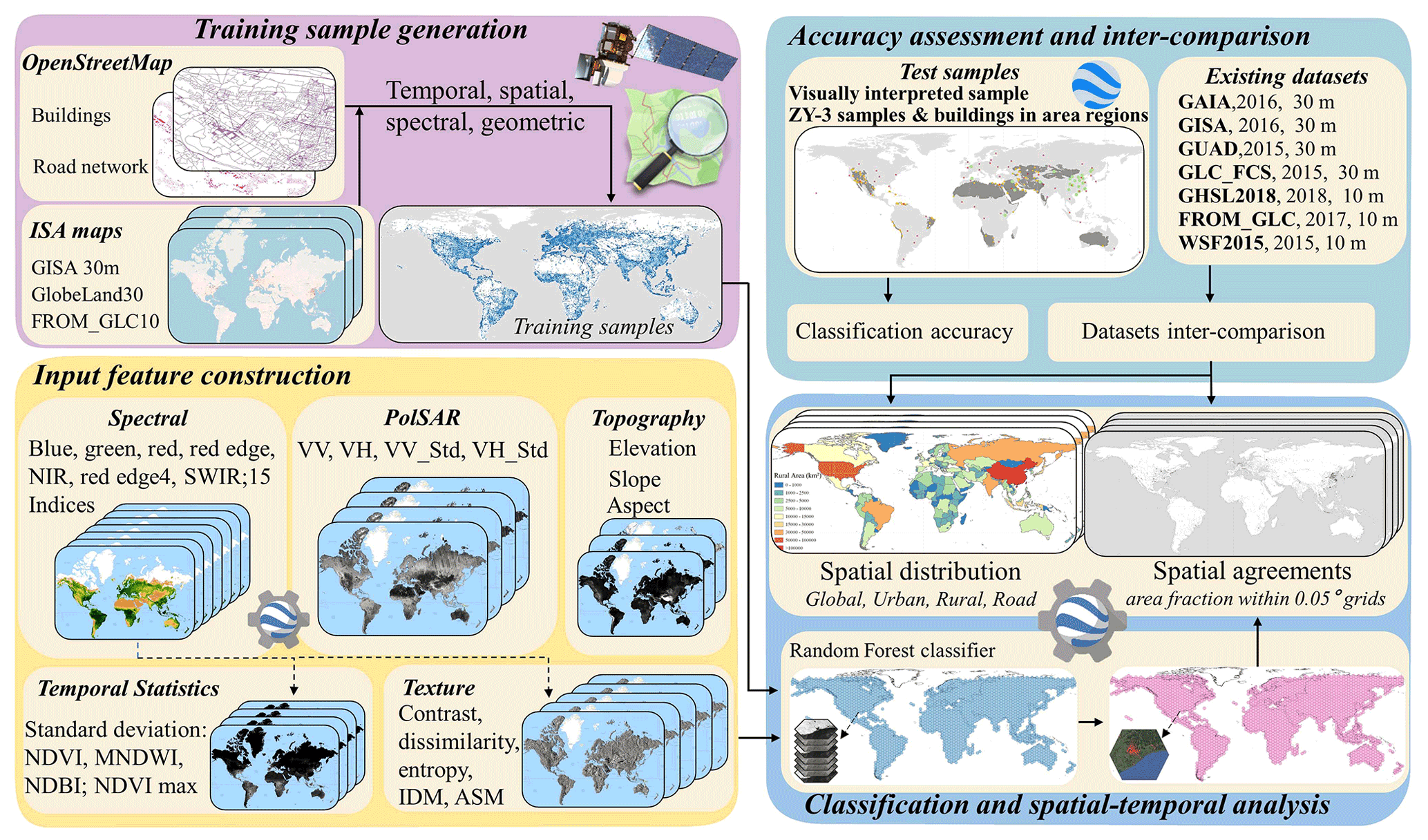
Figure 1 The flowchart for GISA-10m mapping.

3 Methodology

The main objectives of this study were to (1) investigate 10 m global ISA mapping (GISA-10m) by combining Sentinel-1 and 2 images with other geographic information; and (2) analyze the distribution of urban and rural ISA at a 10 m resolution. The flowchart for GISA-10m mapping is shown in Fig. 1, including training sample generation, multi-source feature construction, random forest (RF) classification, accuracy validation, and dataset comparison. Based on the satellite-derived ISA maps and the VGI data (i.e., OpenStreetMap), we proposed a rule-based approach to automatically generate global training samples. Using more than 2.7 million Sentinel images on the GEE, multi-source features were constructed and fed into the RF classifier to obtain the mapping results. The accuracy of the GISA-10m was assessed by visual interpretation and third-party samples. To better evaluate the performance of GISA-10m, we compared it with the current state-of-the-art global ISA datasets (Table 1). Finally, the distribution of ISA over urban and rural regions was analyzed.

3.1 Global ISA mapping using multi-source geospatial data

3.1.1 Sample collection

In the case of large-scale supervised classification, both the quantity and quality of samples are important (Foody and Arora, 1997). ISA is a highly variable object, and its attributes in the Sentinel-2 multispectral images are related to materials, viewing angles, and atmospheric conditions, while its response to the Sentinel-1 SAR instrument depends on dielectric properties, geometry, and surface roughness. Hence, a large number of training samples was required to address the aforementioned challenges that would be encountered at the global scale. Training samples are usually acquired by means of visual interpretation or automatic extraction from the existing datasets. However, the visual interpretation methods are labor- and time-intensive, even for small regions. Therefore, at a large scale, training samples are usually extracted from the existing datasets with similar temporal and spatial coverages. However, the sample quality is affected by the quality of the datasets. Theoretically, samples extracted from a single dataset will result in more errors and uncertainties, while multi-source data can improve the reliability of the training samples (Huang and Zhang, 2013). We therefore proposed to collect global training samples by incorporating the existing ISA datasets and the crowdsourced OSM database. To distinguish the two types of ISA samples, we named the ISA samples extracted from the existing satellite-derived ISA datasets as ISA_RS and those extracted from the OSM as ISA_OSM.

The existing ISA datasets generally cover a broad terrestrial surface, but they differ in terms of their definition, spatial resolution, and temporal coverage. In this study, the GISA, FROM_GLC10, and GlobeLand30 products were chosen to extract the training samples for the following reasons: (1) the GISA is aimed at mapping the global ISA, which is consistent with GISA-10m; (2) the team behind the GlobeLand30 employed extensive visual interpretation to detect artificial surfaces, which can effectively reduce the false alarms from other datasets, i.e., GISA and FROM_GLC10 (Chen et al., 2015); and (3) the definition of FROM_GLC10 (impervious surfaces) is consistent with that of GISA-10m, and its spatial resolution is also 10 m. The GHSL 2018, WSF2015, and GAUD were not considered since they aim to outline human settlements or urban extent (Table 1). We then collected the eligible training samples according to the following rules.

1. Temporal rule. The GISA is a global ISA dataset covering 1972–2019, so we selected its results for 2016 to match the Sentinel data used in this research. GlobeLand30 documents global land cover for 2000, 2010, and 2020, so the 2010 map was chosen in this study. Although the 2020 map is more recent than the 2016 map, it contains ISA that was built after 2016, making it unsuitable for the GISA-10m mapping. Although there is a 6-year gap between GlobeLand30 and the other datasets (i.e., GISA and FROM_GLC10), we adopted the commonly used assumption that the transition from ISA to non-impervious surface area (NISA) rarely happens (P. Gong et al., 2020; Huang et al., 2021b, 2022), so that the GlobeLand30 for 2010 could be used for the GISA-10m mapping. The following spatial and spectral rules were used to remove the possible errors.

2. Spatial rule. We first checked the class labels of the three datasets at each pixel. If these labels were the same (i.e., ISA), the pixel was taken as a potential ISA_RS sample. The incorporation of multiple datasets can effectively reduce the errors that exist in a single dataset. In addition, we filtered out the edge pixels in each dataset to reduce the uncertainty, since they were more likely to be mixed pixels. Edge pixels were defined as the outermost pixels of each ISA patch. We removed the edge pixels in each dataset, and then selected their ISA intersection as potential training samples. In this way, the errors contained in the non-edge pixels in the 30 m resolution data (e.g., mixed pixels) could be removed by the edge pixels in the 10 m resolution data.

3. Spectral rule. After the above steps, a small amount of errors may still remain in the current samples. Hence, we applied the spectral rule to remove these erroneous samples. Specifically, we measured the Mahalanobis distance between each ISA_RS sample to the spectral average of each hexagon (the mapping unit adopted in this study), and filtered out the samples with a distance greater than μ+δ (where μ and δ represent the mean and standard deviation, respectively) (Huang et al., 2021b). Vegetation and water bodies are common sources of false alarms in the existing datasets (Fig. 2a and b). However, these errors often account for a relatively small proportion, and they can be effectively identified and reduced by the spectral rule. It can be seen in Fig. 2 that most of the water bodies and vegetation (the red rectangles in Fig. 2) were successfully removed from the initial ISA_RS training samples.

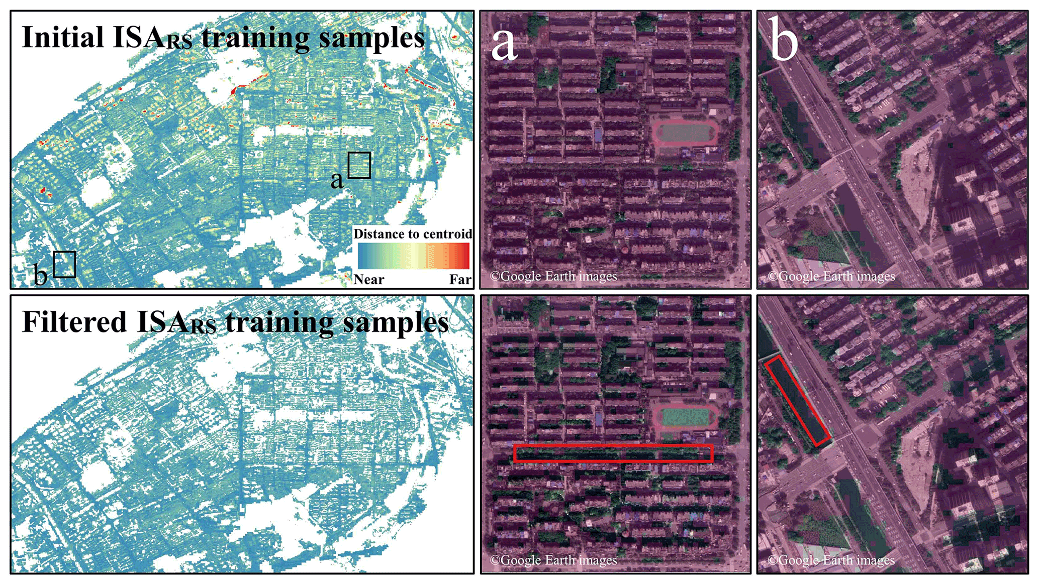
Figure 2 Examples of the initial and filtered ISA_RS training samples from the city of Wuhan in China (30.625382^∘ N, 114.392682^∘ E). The purple in the close-up maps represents the samples.

We extracted the ISA_OSM samples from the OSM buildings and roads through the following rules.

1. Temporal rule. We chose the OSM data built on 2 January 2017 in terms of the time of GISA-10m. This version of the OSM data was employed to ensure that the buildings and roads were constructed in 2016 or before, and hence were suitable for the 2016 ISA mapping.

2. Geometric rule. A natural way to extract training points from OSM data is to generate random points within the building or road polygons (D. Liu et al., 2020). However, random points may contain erroneous or mixed pixels. Such problems can be mitigated by applying negative buffers to the polygons (D. Liu et al., 2020a). However, this approach is very time-consuming when applied to global ISA mapping, especially given the more than 200 million buildings in the OSM database. Therefore, in this study, we extracted the geometric center of a building polygon as an ISA_OSM sample, which was more efficient than buffering or random points. Notably, although we could filter out the erroneous buildings using attribute tags (e.g., dams, swimming pools, playgrounds), the geometric center of a building was not always an ISA sample. Hence, we further required that the geometric center must be contained by the building. As in Fig. 3a and b, the incorrect building geometric centers (e.g., the vegetation and water, as indicated by the yellow points) were successfully identified and removed by the geometric rule. In addition, we excluded buildings with an area of less than 100 m² (approximately a Sentinel pixel), to ensure the reliability of the samples. This is because a training sample extracted from the geometric center may be NISA when the area of the building is smaller than a Sentinel pixel.

   Compared with the widely used 30 m Landsat data, the high-resolution Sentinel data allow a better delineation of roads. We thereby also extracted ISA_OSM samples from the OSM road networks. The OSM roads usually consist of centerlines rather than boundaries. Therefore, we extracted the center point of each road, rather than its geometric center, as the road ISA samples. Given that the width of low-grade roads may be less than 10 m (i.e., a Sentinel pixel), we kept only the main roads (highway = “primary”).

3. Spatial rule. Given the uneven spatial distribution of OSM data (Tian et al., 2019), we applied the spatial rule to balance the distribution at the global scale. Specifically, for hexagons with more than 10 000 OSM records (i.e., buildings and roads), we randomly selected 10 000 records as initial samples. The dilution of OSM data can significantly reduce the subsequent computational cost. In the field of supervised classification, the diversity of the samples is important for the generalization ability of the classification model (Huang and Zhang, 2013). Considering that ISA_OSM can overlie with ISA_RS, we removed the ISA_OSM samples intersected with the ISA_RS sample pool to increase the diversity and reduce the redundancy of the ISA samples.

4. Spectral rule. Although OSM uses humans as sensors, ISA_OSM samples can still contain erroneous points, such as vegetation and water bodies, in addition to roads. As shown in Fig. 3c and d, the yellow points satisfy the temporal, spatial, and geometric rules, but they are actually vegetation. Hence, we applied the spectral rule to filter out these erroneous points. Specifically, the ISA_OSM samples whose modified normalized difference water index (MNDWI) or normalized difference vegetation index (NDVI) value was larger than μ+δ were removed (μ and δ represent the mean and standard deviation of the indices, respectively), as these points were more likely to be vegetation or a water body (Huang et al., 2021b).

   After obtaining the ISA candidate samples, we randomly selected 2500 ISA_RS and ISA_OSM samples, respectively, within each hexagon as the final ISA training samples (see Sect. 5.3 for details). It can be seen that the generated ISA samples cover a broad terrestrial surface, especially in India and China, where a large number of small villages are found (Fig. 4).

Figure 3 Examples of the initial and filtered ISA_OSM training samples from the city of Wuhan in China (30.530202^∘ N, 114.356287^∘ E). The yellow points in the close-up maps represent the errors recognized by (a–b) the geometric rule and (c–d) the spectral rule.

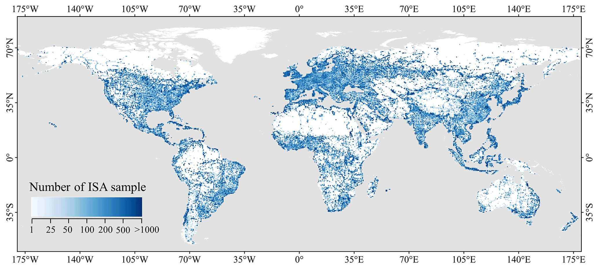
Figure 4 Global distribution of ISA training samples. The number of samples was counted within 0.5^∘ spatial grid.

On the other hand, NISA (non-ISA) training samples are also important for accurate ISA mapping. We used the three existing datasets (i.e., GISA 30 m, FROM_GLC10, GlobeLand30) and the OSM to generate the NISA samples. Firstly, we took the intersection of the NISA regions in the three datasets as the initial NISA sample pool:

$$\begin{array}{}\text{(1)}& \begin{array}{rl}\mathrm{NISA}& ={\mathrm{NISA}}_{\mathrm{GISA}}\cap {\mathrm{NISA}}_{\mathrm{GlobeLand}\mathrm{30}}\\ & \cap {\mathrm{NISA}}_{\mathrm{FROM}\mathrm{\_}\mathrm{GLC}\mathrm{10}}-{\mathrm{ISA}}_{\mathrm{OSM}}.\end{array}\end{array}$$

For GlobeLand30 and FROM_GLC10, NISA is defined as all the land-cover types other than ISA. We masked the initial NISA sample pool using the OSM buildings and roads to suppress the errors in the existing global datasets. To this end, we used the OSM version built in December 2020 (https://planet.openstreetmap.org/planet/2020/planet-201207.osm.bz2, last access: 13 March 2021), which documents more buildings and road networks than the 2017 version. In addition, we buffered the OSM roads with a 30 m buffer to mitigate the errors. Subsequently, 30 000 points were randomly selected in each hexagon as NISA samples. The distance between each NISA sample was kept larger than 200 m to ensure the diversity and irrelevance. Finally, we extracted 58 million training samples (51 674 533 NISA samples and 6 897 378 ISA samples) for the GISA-10m mapping.

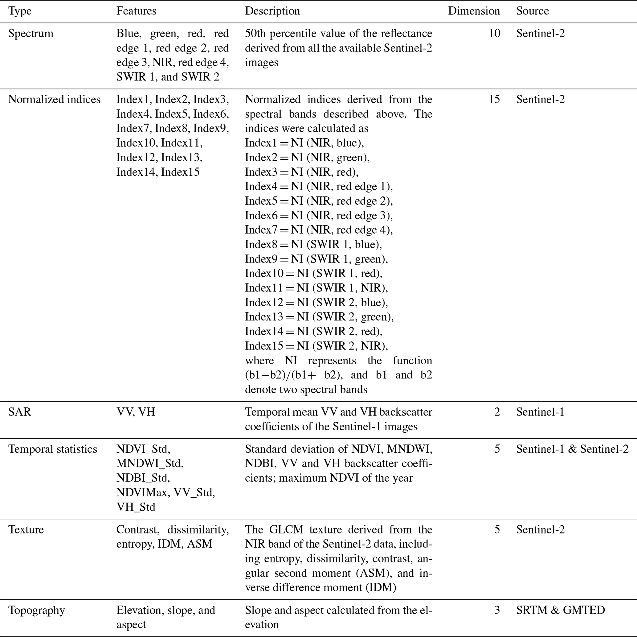
Table 2 The multi-source features used for the GISA-10m mapping.

3.1.2 Multi-source feature extraction

The dedicated image pyramid of the GEE platform enabled us to perform pixel-wise feature extraction (Gorelick et al., 2017). Therefore, based on all the available Sentinel data for 2016, we constructed a set of spectral, phenological, textural, SAR, and topographical features with the temporal composite method (Table 2). This approach used all the available data and, at the same time, allowed us to reduce the feature dimension, preserve the temporal information, and minimize the effects of clouds and shadows (Yang and Huang, 2021). Firstly, we used the spectral signatures provided by the Sentinel-2 data to extract the ISA in the visible, red-edge, NIR, and infrared bands (Table 2). Moreover, considering that spectral indices can increase the differences between land covers, we also extracted a series of normalized spectral indices to enhance the discriminative ability between ISA and NISA (Yang and Huang, 2021) (Table 2). These indices were built according to the following criteria: (1) they were mainly constructed by the NIR and SWIR bands due to their better atmospheric transmission (Huang et al., 2021b; Yang and Huang, 2021); and (2) each index contained at least one 10 m band (i.e., visible and NIR bands) to ensure the spatial resolution of the features.

The complex spectral and spatial characteristics in urban environments increase the difficulty of ISA mapping. In this regard, textural features are usually employed to depict the spatial information of urban ISA (Huang and Zhang, 2013). To further exploit the textural information for the ISA mapping, we computed the gray-level co-occurrence matrix (GLCM) via the NIR band to depict the spatial information of urban ISA. Owing to the high redundancy among GLCM measurements (Clausi, 2002), we chose the contrast, dissimilarity, entropy, inverse difference moment (IDM), and angular second moment (ASM) for the texture extraction (Rodriguez-Galiano et al., 2012). The window size for the GLCM measurements was set to 7 × 7 as this is suitable for urban classification with an image resolution from 2.5 to 10 m (Puissant et al., 2005). In addition, we averaged the GLCM from different directions (0, 45, 90, and 135^∘) to maintain the rotational invariance (Rodriguez-Galiano et al., 2012).

Given that the spectra and backscatter of some NISA (e.g., vegetation and water bodies) vary throughout time, the phenological information derived from the multi-temporal spectral and SAR data was utilized to depict the temporal fluctuations. We calculated the maximum NDVI and the standard deviation of the NDVI (Tucker, 1979), MNDWI (Xu, 2006), and normalized difference built-up index (NDBI) (Zha et al., 2003), to further enhance the temporal information. These temporal characteristics are useful in identifying NISA with temporal fluctuations. For example, the spectra of fallow cropland and ISA are similar, and even SAR data may not separate them well. However, the NDVI of cropland can describe the changes of crop growth, and hence its standard deviation can be used to distinguish between ISA and cropland. In addition, to increase the robustness of these temporal features, Sentinel-2 data from two adjacent years were also considered.

SAR data have the potential to reduce the false alarms caused by bare soil in optical images, and are more sensitive to buildings. In addition, SAR signals can penetrate clouds. Therefore, in this study, SAR data were combined with optical data for the ISA mapping. Specifically, the vertical–vertical (VV) polarization and the vertical–horizontal (VH) polarization backscatter coefficients from the Sentinel-1 images were selected. Based on all the available Sentinel-1 data, the annual mean and standard deviation of the VV and VH backscatter coefficients were calculated by the temporal composite method:

$$\begin{array}{}\text{(2)}& {\displaystyle }{\mathit{\sigma }}_{\mathrm{mean}}& {\displaystyle }={\displaystyle \frac{\mathrm{1}}{n}}{\sum }_{i=\mathrm{1}}^n{\mathit{\sigma }}_i\text{(3)}& {\displaystyle }{\mathit{\sigma }}_{\mathrm{std}}& {\displaystyle }=\sqrt{{\displaystyle \frac{{\sum }_{i=\mathrm{1}}^n({\mathit{\sigma }}_i-{\mathit{\sigma }}_{\mathrm{mean}}{)}^{\mathrm{2}}}{n}}},\end{array}$$

where n denotes the total number of Sentinel-1 observations within a year, and σ_i represents the ith backscatter coefficient observation in the year. The temporal composite method can reduce the speckle noise in SAR imagery (Lin et al., 2020), while the annual standard deviation can reflect the temporal information. Topography-related features are also necessary for ISA mapping in order to reduce the confusion between complex terrain and buildings. For instance, topographical features can help to distinguish steep hills from buildings (Gamba and Lisini, 2013). Specifically, we used Shuttle Radar Topographic Mission (SRTM) digital elevation model (DEM) data in the areas below 58^∘ latitude, and Global Multi-resolution Terrain Elevation Data 2010 (GMTED2010) in the areas above 58^∘ (Huang et al., 2021b). Finally, a total of 41 features were constructed from the 2.7 million Sentinel images (2 613 180 Sentinel-2 and 122 156 Sentinel-1) and DEM data.

3.1.3 Hexagon-based adaptive random forest classification

When dealing with global land-cover classification, the global terrestrial surface is usually divided into homogeneous sub-regions according to criteria such as climate, land cover, or administrative regions (Goldblatt et al., 2018). For global ISA mapping, regular square grids are commonly used (Table 1), such as 1 and 5^∘ grids (e.g., WSF2015 and GLCFCS). In this study, we divided the terrestrial surface into 2^∘ hexagonal grid cells (Fig. 1) due to the symmetry and invariance (You et al., 2021). Furthermore, there were no gaps or overlaps between hexagons, and the distance between adjacent hexagon centers was approximately equal (Richards et al., 2000).

The RF classifier has been widely used in global ISA mapping due to its robustness to erroneous samples, flexibility with high-dimensional data, and tolerance to noise (Bauer and Kohavi, 1999; Wulder et al., 2018) (Table 1). The RF classifier utilizes ensemble learning to obtain predictions by voting on categories through multiple decision trees (Breiman, 2001). Each tree uses a random subset of the input features to increase the generalization ability. In addition, trees are grown from different subsets of training data (i.e., bagging or bootstrapping) to increase the diversity (Rodriguez-Galiano et al., 2012). RF has been shown to outperform other classifiers when dealing with large-scale and high-dimensional data (Goldblatt et al., 2016). The ability of RF to handle multi-source data also makes it convenient when dealing with Sentinel radar and optical data. Therefore, together with the aforementioned multi-source features and global training samples, the RF classifier was used for the GISA-10m mapping. As suggested by Yang and Huang (2021), the number of trees was set to 200. We divided the global terrestrial surface into 1808 hexagons, and a local RF model was built for adaptive ISA classification in each hexagon. Therefore, a total of 1808 RF models were built. In terms of the features used to train each tree, the random forest uses a random subset of features to reduce the correlation between trees. In general, the diversity of the trees can be increased when fewer features are used for training each tree (Breiman, 2001). In the GISA-10m mapping, we set the number of features used for each tree to the square root of the total number of features, as suggested by H. Liu et al. (2020).

3.2 Accuracy assessment

The test samples for GISA-10m included (1) visually interpreted samples via Google Earth; (2) test samples extracted from ZiYuan-3 (ZY-3) built-up datasets (Liu et al., 2019); and (3) building samples located in arid areas.

1. As suggested by Stehman and Foody (2019), we used cluster sampling to collect the visually interpreted test samples. The primary sampling unit involved 59 grid cells with a side length of 1^∘, which were randomly selected based on population, ecoregion, and urban landscape (the red squares in Fig. 5). The secondary sampling unit included the random samples within each grid cell. In such a way, samples from different urban sizes and densities were considered for the validation. Specifically, in each grid cell, we randomly selected 100 ISA and 100 NISA points to test their accuracy. An equal allocation of ISA and NISA test samples could reduce the bias of the accuracy assessment, and hence allow for a more accurate estimation of the user's accuracy (Olofsson et al., 2014; Stehman, 2012). By referring to high-resolution Google Earth images, a pixel (10 m × 10 m) was labeled as ISA if more than half of its area was covered by ISA; otherwise, it was identified as NISA. As can be seen in Fig. 5, the test samples involved not only high-density ISA samples from urban areas, but also a large number of low-density samples from suburban and rural regions. Finally, a total of 11 800 test samples were obtained.

2. Liu et al. (2019) proposed a multi-angle built-up index to extract built-up areas from ZY-3 images covering 45 global cities, which obtained an overall accuracy (OA) of greater than 90 %. The multi-angle ZY-3 images depict the three-dimensional and vertical structure of buildings, which is more effective and accurate than planar feature extraction for detecting built-up areas. Given the higher spatial resolution (2 m) and better accuracy of the ZY-3 global built-up dataset, we extracted test samples from it for the year of 2016 (Huang et al., 2021b; Liu et al., 2019). A sample (10 m × 10 m) was labeled as ISA if more than 50 % of its area was classified as ISA in the ZY-3 dataset, while the NISA samples were those with no built-up pixels in the area (Huang et al., 2021b). For each city, the number of samples was proportional to the area of the ZY-3 image, and the ratio of ISA and NISA test samples was consistent with the ratio of the built-up and non-built-up classes (Huang et al., 2021b). In this way, we obtained 47 216 NISA samples and 21 152 ISA samples (the green dots in Fig. 5) from 24 cities in the ZY-3 built-up dataset.

3. Considering the difficulty of ISA extraction in arid regions (Tian et al., 2018), we paid special attention to the accuracy assessment in the arid regions. To this end, we visually interpreted 5385 building pixels in these regions. A total of 25 photo interpreters were recruited for this task by referring to the Google Earth images. These samples were then further checked by three experts. The arid regions were defined according to the “deserts and xeric shrublands” biome in Olson et al. (2001).

   Based on the three groups of test samples aforementioned, the accuracy of GISA-10m was assessed using the OA, kappa, producer's accuracy (PA), user's accuracy (UA), and F1-score (the harmonic mean of the PA and UA). Seven existing global ISA datasets were used for the inter-comparison with GISA-10m, i.e., GHSL 2018, GLCFCS, WSF2015, FROM_GLC10, GISA, GAUD, and GAIA (Table 1). The three groups of test samples mentioned above were used to assess and compare the accuracy of these products.

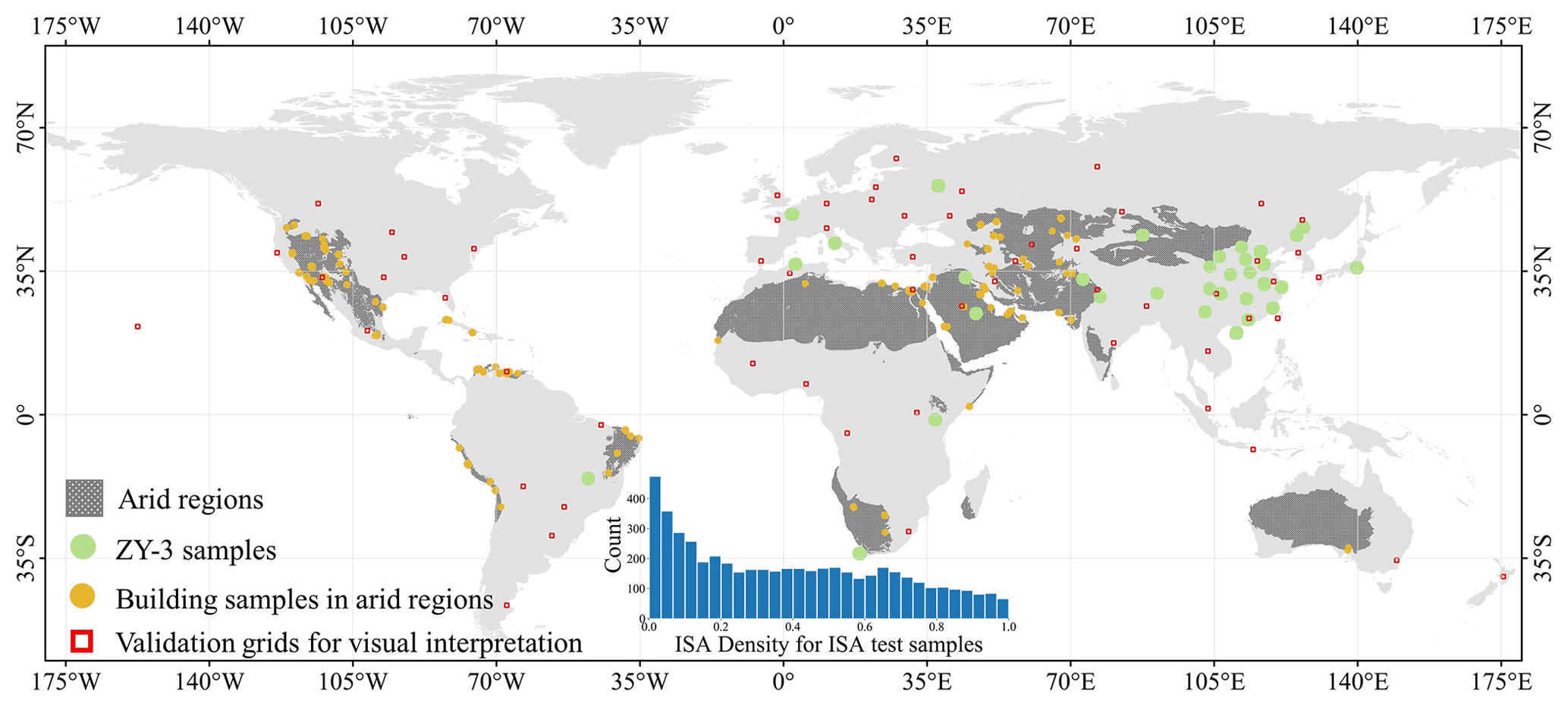
Figure 5 Global distribution of the test samples and grid used in this study, including (1) 59 grids for visual interpretation, (2) ZY-3 reference set covering 23 cities, and (3) 5385 building samples in the arid regions. The arid regions were extracted from “deserts and xeric shrublands” biome in Olson et al. (2001). The inner graph shows the ISA density within the 0.5 km buffer for the ISA test samples.

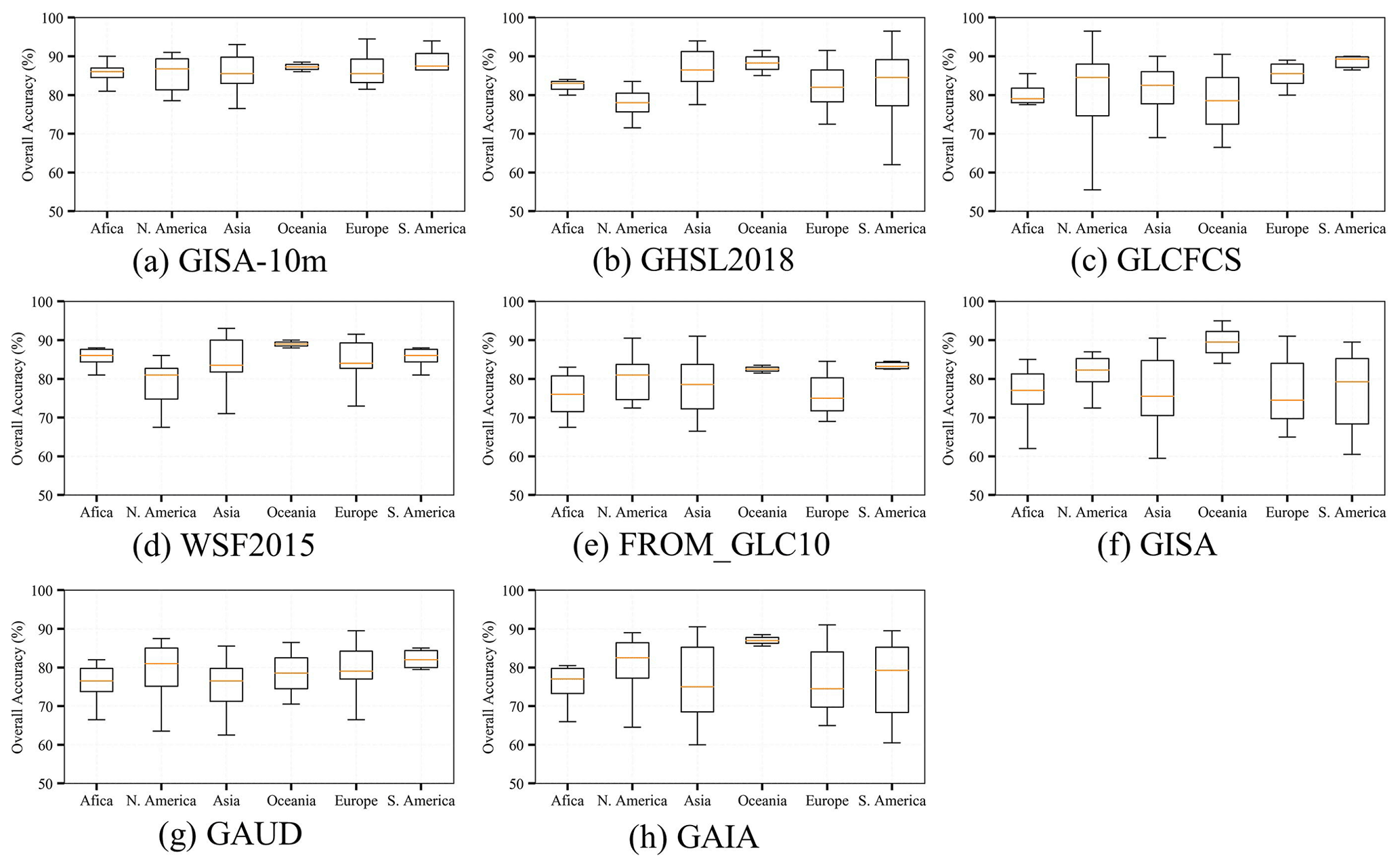
Figure 6 Box plots of the overall accuracy for GISA-10m and existing datasets in the six continents.

4 Results

4.1 Accuracy assessment of GISA-10m

4.1.1 Global scale

The accuracy assessment based on the visually interpreted samples is shown in Table 3. GISA-10m exhibits the highest OA of 86.06 %, representing an increase in OA of +2.73 %, +3.73 %, and +2.3 % over GHSL 2018, GLCFCS, and WSF2015, respectively (Table 3). The kappa of GISA-10m is 0.7165, which exceeds WSF2015, FROM_GLC10, and GAIA by 0.052, 0.1774, and 0.2039, respectively. GISA-10m also shows a higher accuracy than the 30 m resolution datasets (i.e., GISA, GAUD, GAIA), which suggests a better delineation of global ISA due to the higher resolution. Figure 6 summarizes the results of the accuracy assessment at the continent level, with the average and standard deviation of the OA for each continent shown in the box plots. Overall, GISA-10m exhibits a stable performance for each continent with an average OA of more than 85 %. Specifically, Oceania and South America show the best OAs of 87.25 % and 87.08 %, followed by Europe (86.45 %) and Asia (85.85 %). The results also show that the average OA of GISA-10m exceeds that of the existing datasets in Africa, North America, and Europe. In addition, it is apparent that the performance of GHSL 2018 and GLCFCS is relatively unstable in South America and North America, respectively.

Table 3 Results of quantitative accuracy assessment via visually interpreted and ZY-3 samples between GISA-10m and the existing ISA datasets. OA represents the overall accuracy. Bold numbers represent the highest value for each metric.

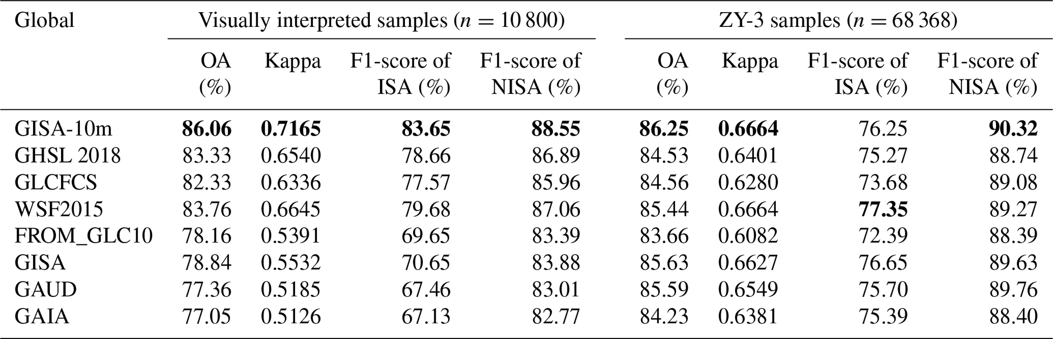
GISA-10m obtains the best OA of 86.25 % on the ZY-3 samples, outperforming GHSL 2018, GLCFCS, and WSF2015 by 1.72 %, 1.69 %, and 0.81 %, respectively. The ZY-3 images employed by Liu et al. (2019) covered 45 major global cities, and therefore the ZY-3 samples were more inclined to reflect the accuracy in urban regions. Therefore, the accuracy difference between the various datasets is not significant (Table 3). Due to the relatively coarse resolution, the 30 m datasets usually tend to overestimate the ISA extent (P. Gong et al., 2020), resulting in a higher UA but lower PA (Table S1 in the Supplement). For example, the ISA UA of GISA is slightly higher than that of GISA-10m, but its PA is much smaller (Table S1). However, when the two metrics (PA and UA) are considered at the same time (i.e., the F1-score), GISA-10m outperforms GISA.

4.1.2 Rural, arid, and urban regions

The population of rural regions is comparable to that of urban regions (https://data.worldbank.org/, last access: 9 August 2022). The existing studies, and their global ISA datasets, have usually focused on the performance in urban regions, and the accuracy of the rural ISA regions has not been sufficiently assessed. Hence, in this study, we paid special attention to the accuracy assessment in the global rural regions. Specifically, we divided the GISA-10m into urban and rural regions using the urban boundary defined by Li et al. (2020). In fact, due to the random sampling strategy, most of the visually interpreted test samples were located in rural regions.

In the case of the visually interpreted samples, GISA-10m exhibits a better OA of 86.19 % than GHSL 2018 (84.92 %), GLCFCS (83.25 %), FROM_GLC10 (78.83 %), and WSF2015 (83.81 %). As regards the three 30 m datasets (i.e., GISA, GAIA, GAUD), their ISA accuracy (F1-score) decreases significantly in the rural regions, while the NISA accuracy is relatively stable (Tables 2–3). Taking a closer look at the PA, it is apparent that the ISA PA decreases by more than 15 % for all three 30 m datasets (Table S2), which suggests that there are more omission errors in the rural regions (Fig. 11b). This demonstrates the deficiency of the 30 m datasets in depicting rural ISA, and also reflects the importance of 10 m global ISA mapping.

Table 4 Results of quantitative accuracy assessment via visually interpreted and ZY-3 samples in rural regions between GISA-10m and the existing ISA datasets. OA represents the overall accuracy. Bold numbers represent the highest value for each metric.

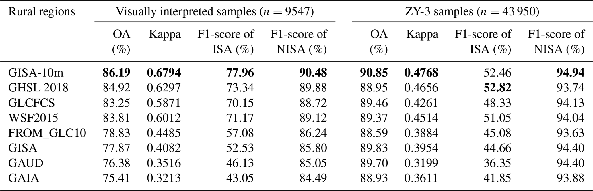
Table 5 Results of quantitative accuracy assessment via visually interpreted and ZY-3 samples in arid regions between GISA-10m and the existing ISA datasets. OA represents the overall accuracy. Bold numbers represent the highest value for each metric.

Furthermore, we also focused on the accuracy assessment in arid regions. In general, the OA of GISA-10m is higher than that of the existing datasets (Table 5). Although its ISA UA does not always outperform the other datasets, GISA-10m achieves the highest PA (Table S4). Specifically, GISA-10m exhibits a notably higher ISA PA than GLCFCS, FROM_GLC10, GISA, GAUD, and GAIA (Table S3), indicating its superior ability to detect ISA in arid regions (Fig. 7). Moreover, the accuracy of these global ISA products was assessed using the manually and randomly chosen rural building samples (see Sect. 3.2). It can be found that GISA-10m detects 15 % more buildings in arid regions than FROM-GLC10, GAUD, and GAIA (Table S5), which further verifies its superior performance in describing rural ISA.

In the case of urban regions, GISA-10m exhibits a satisfactory result, with an OA similar to that of the global assessment (Table S4). Note that urban ISA only accounts for one-third of global ISA, while nearly 70 % of ISA is located in suburban and rural regions. The existing datasets show relatively more ISA omissions in rural and arid regions, suggesting that global ISA mapping at a 10 m resolution (e.g., GISA-10m) is necessary. Moreover, we divided the visually interpreted samples located in cities into three levels (i.e., small, medium, and large cities) to assess the accuracy of GISA-10m for cities of different scales, i.e., Level 1 (population < 250 000), Level 2 (250 000 to 1 000 000), and Level 3 (> 1 000 000) (Yang et al., 2019). The OA of GISA-10m across the three levels of cities is 85.35 %, 87.43 %, and 85.42 %, respectively (Table S6). These results indicate that the performance of GISA-10m in different scales of cities is stable, and the results are also close to the global assessment result (OA of 86.06 %).

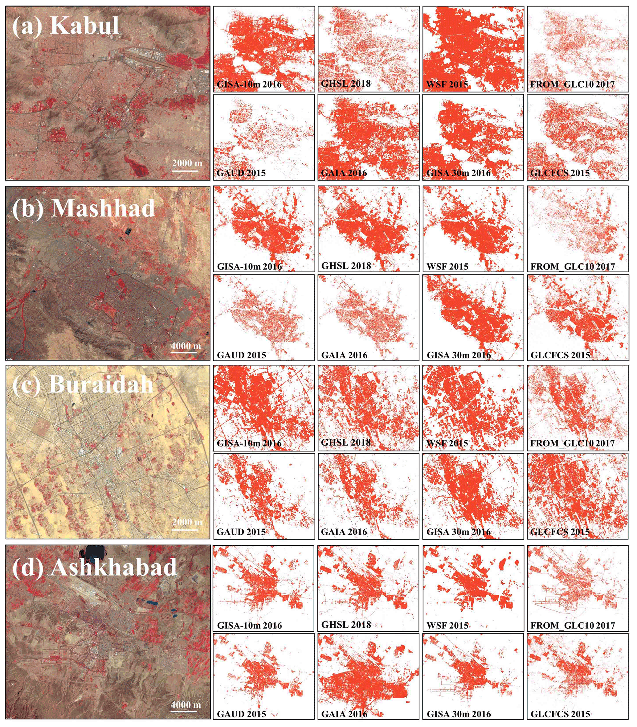
Figure 7 Comparison of the GISA-10m and the other datasets over arid regions in (a) Kabul, Afghanistan; (b) Mashhad, Iran; (c) Buraidah, Saudi Arabia; and (d) Ashkhabad, Turkmenistan. The illustration is of Sentinel-2 images with a false-color combination (R: NIR, G: red, B: green) to enhance the ISA.

4.2 Global ISA distribution

4.2.1 Urban and rural ISA

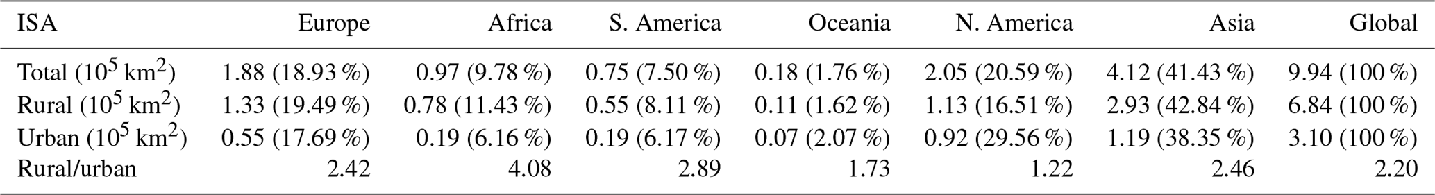
Based on the GISA-10m, we analyzed the global ISA distribution at a 10 m scale (Fig. S1). Global ISA is mainly distributed in Asia (41.43 %), North America (20.59 %), and Europe (18.93 %), followed by Africa (9.78 %) and South America (7.50 %). It is found that 67 % of global ISA is located in the Eastern Hemisphere, while 85 % of ISA is distributed to the north of the Equator. Rural ISA is more scattered than urban ISA (Fig. S1), and is mainly located in Asia (42.84 %), Europe (19.49 %), and North America (16.51 %). Asia has the largest urban ISA, which is more than twice that of Europe. Although North America only accounts for 20 % of global ISA, its urban ISA takes up more than 29 % of the global total. Taking a closer look at the ratio of rural and urban ISA (Table 6), it can be seen that rural ISA is 2.2 times larger than urban ISA. At the continental level, Africa possesses the highest “rural-to-urban ratio”, which is likely related to its large population but relatively poor economy.

Table 6 Impervious surface area derived from GISA-10m in the six continents.

At the country scale, China and the US account for 33 % of global ISA. Together with Russia, Brazil, India, Japan, Indonesia, France, Canada, and Germany, these 10 countries account for 58 % of the world ISA. The urban ISA of the top 10 countries (US, China, Russia, Brazil, Japan, India, Mexico, France, Germany, and the United Kingdom) makes up 69 % of the global total, while the top 10 countries in terms of rural ISA (China, US, Russia, Brazil, India, Indonesia, Japan, France, Canada, and Germany) account for only 54 % of the total (Fig. S3). In Africa, the Republic of South Africa has much more urban ISA than the other countries. However, Nigeria has a comparable rural ISA to South Africa (∼ 7738 km²). China ranks first in terms of rural ISA, most of which is located in the North China Plain (Fig. S1b). Indonesia also possesses a lot of rural ISA, since it ranks sixth for rural ISA but only 16th for urban ISA.

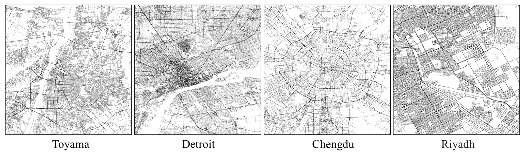
Figure 8 Examples of road area derived from GISA-10m and OSM in Toyama (Japan), Detroit (US), Chengdu (China), and Riyadh (Saudi Arabia).

4.2.2 Global road area

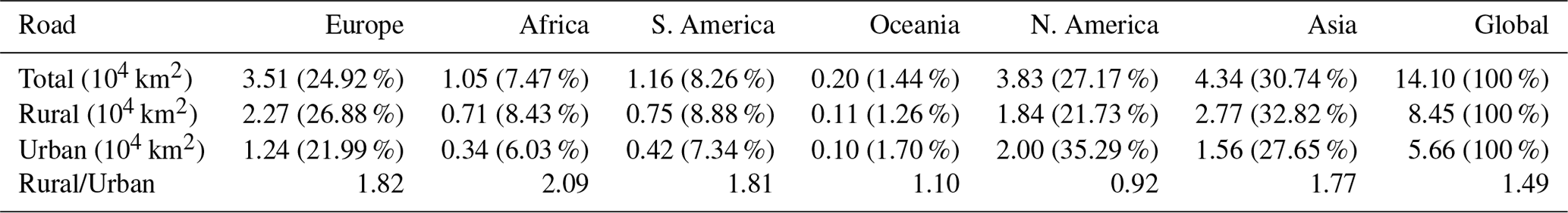
Roads are major anthropic footprints, so we attempted to analyze the global road area based on GISA-10m, courtesy of its high spatial resolution. Firstly, the road networks were extracted from the OSM database, and then the ISA regions in the GISA 10 m data within a 10 m buffer of the road networks were identified as road areas (Fig. 8). The results show that 82.84 % of the global road area is located in Asia (30.74 %), North America (27.17 %), and Europe (24.92 %), while the remaining 17.16 % is found in South America (8.26 %), Africa (7.47 %), and Oceania (1.44 %). Although Asia far exceeds the other continents with regard to ISA and rural road area, it possesses a smaller urban road area than North America. China and the US have the largest road area, together accounting for 29 % of the global total, followed by Brazil, Japan, Russia, Germany, India, France, Indonesia, and Mexico. The top 10 countries have more than half of the global road area. The global road area accounts for 14.18 % of the global ISA, and the rural road area is 1.5 times larger than the urban road area (Table 7). However, it should be noted that these estimates might be biased owing to the incompleteness of the OSM data. In addition, narrow roads might be partly detected or missed due to the limitation of the spatial resolution.

Table 7 Statistics for the road area derived from GISA-10m and OSM in the six continents.

5 Discussions

5.1 Inter-comparison with the existing datasets

To further validate the performance of GISA-10m, we compared it with the existing state-of-the-art global datasets, i.e., three 10 m resolution datasets (WSF2015, GHSL 2018, FROM_GLC10) and four 30 m resolution datasets (GLCFCS, GAUD, GAIA, GISA). Their spatial agreement with GISA-10m was measured by the linear fit of the ISA fraction, including metrics such as the correlation coefficient and root mean square error (RMSE). Attention was also paid to the performance of the different products in urban and rural regions for a comprehensive assessment. Considering the different spatial resolutions, the ISA fraction was calculated within the 0.05^∘ spatial grid.

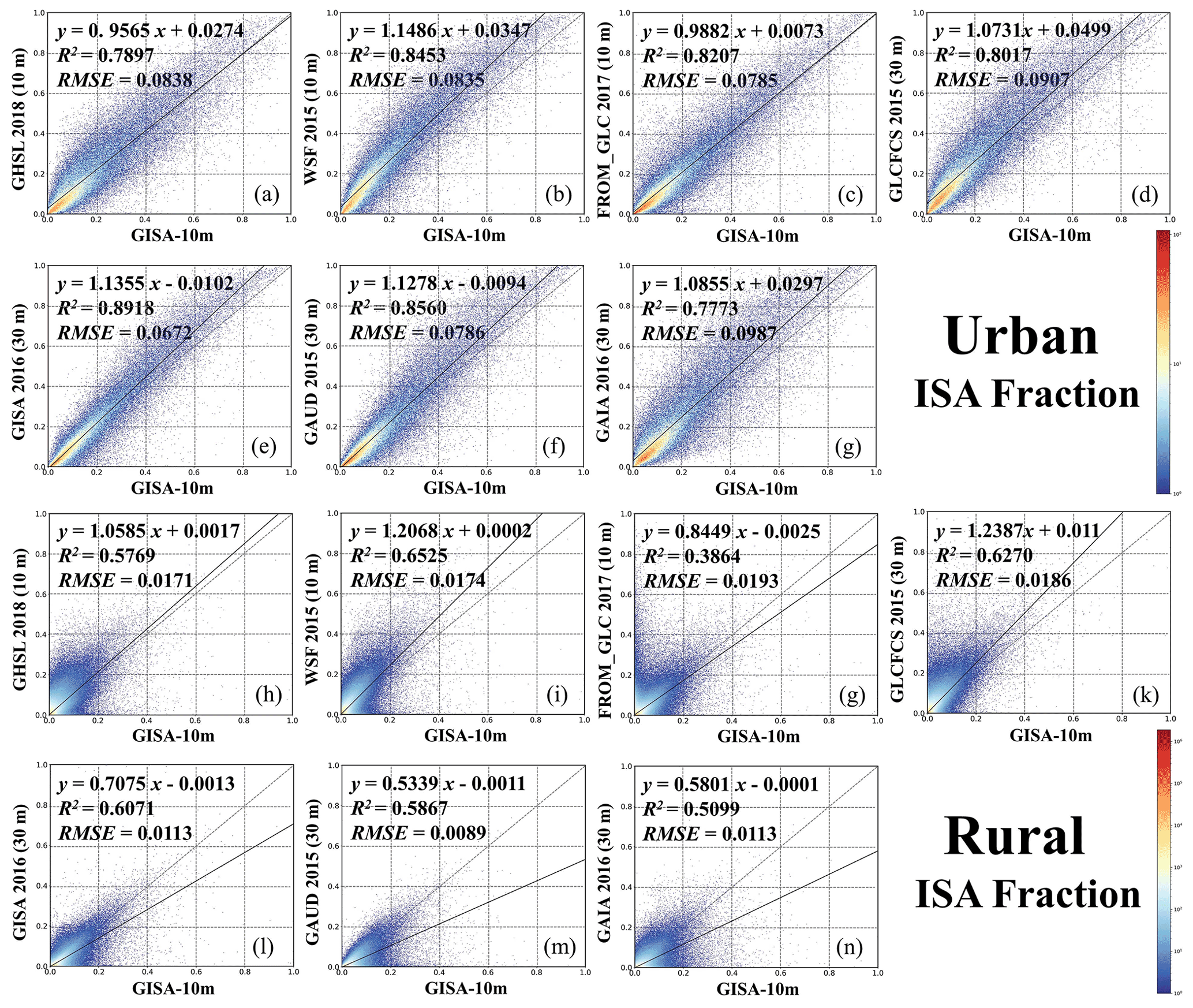
Figure 9 Scatterplots of the urban and rural ISA fraction between GISA-10m with GHSL, WSF, FROM_GLC10, GLCFCS, GAUD, GAIA, and GISA, respectively. The ISA fraction was calculated within a 0.05^∘ × 0.05^∘ spatial grid.

In general, GISA-10m exhibits a high agreement (0.777 < R² < 0.892) with these existing datasets over urban regions. In the case of GHSL 2018 and FROM_GLC10, their fitted lines with GISA-10m are closer to the 1:1 line in the high fraction regions (Fig. 9a and c). As shown in Fig. 10, GHSL 2018 and GISA-10m are generally similar in the dense urban areas (e.g., the urban cores in Fig. 10), but GHSL 2018 tends to overestimate ISA in the low-density residential areas (Fig. 10c). The fitted lines for GLCFCS and WSF2015 are above the diagonal (slope greater than 1 and intercept greater than 0) in both the high and low ISA fraction regions, possibly due to their overestimation. For instance, in the case of Cairo (Fig. 10b), WSF2015 shows significant overestimation, but the other datasets better depict the residential areas. According to Marconcini et al. (2020a), the overestimation of WSF2015 may be related to the employment of the coefficient of variation (COV), which reduces the omissions in the rural regions, but at the same time leads to overestimation of the ISA extent. The fitted lines for the three 30 m resolution datasets (i.e., GISA, GAIA, GAUD) are all above the diagonal (Fig. 9e–g), suggesting that they detect more urban ISA than GISA-10m. However, in the 30 m resolution datasets, vegetation alongside roads or buildings is often identified as ISA due to the issue of mixed pixels (P. Gong et al., 2020). From this perspective, the results of GISA-10m appear more reliable due to its higher spatial resolution. For instance, in the case of Johannesburg and Los Angeles (Fig. 10c and d), GAIA and GAUD exhibit false alarms in both residential and industrial areas, but these errors are significantly reduced in GISA-10m, due to the superior discriminative ability of the 10 m Sentinel data.

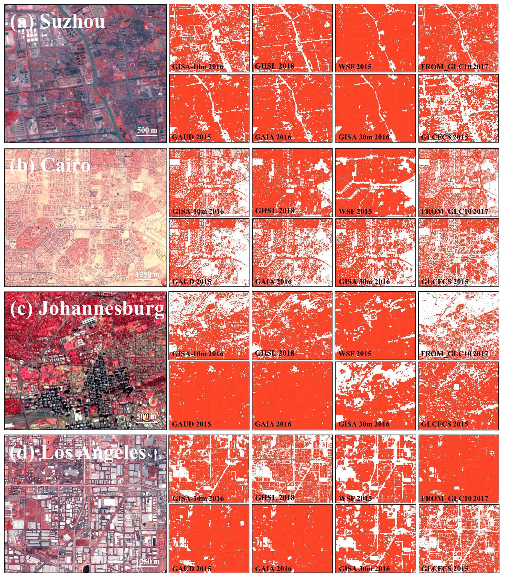
Figure 10 Comparison between GISA-10m and the seven datasets over urban regions in (a) Suzhou, China; (b) Cairo, Egypt; (c) Johannesburg, South Africa; and (d) Los Angeles, US. The Sentinel-2 images were composited in a false-color combination (R: NIR, G: red, B: green).

On the other hand, the agreement between GISA-10m and the existing datasets is slightly lower in rural regions (0.5099 < R² < 0.6525). The fitted slopes between the three 30 m datasets (i.e., GISA, GAIA, GAUD) and GISA-10m in the rural regions are all less than one. This phenomenon can be attributed to the finer spatial resolution of GISA-10m, which detects more rural ISA than the 30 m datasets (Fig. 11b and d). As for GLCFCS and WSF2015, they possess more rural ISA than GISA-10m (Fig. 9i and k), which could be attributed to their overestimation. For example, in Fig. 11a and c, GLCFCS and WSF2015 fail to identify the vegetation in the village. FROM_GLC10 appears more consistent with GISA-10m (see the sample from the US in Fig. 11d), but it tends to underestimate the rural ISA (see Fig. 11a–c). GHSL 2018 and GISA-10m show high agreement in rural regions. However, GHSL 2018 is aimed at outlining human settlements, while GISA-10m is focused on artificial ISA (including buildings, parking lots, and roads).

Figure 11 Comparison between GISA-10m and the seven datasets over rural regions in (a) China (126.348044^∘ E, 45.269079^∘ N); (b) Uzbekistan (60.573313^∘ E, 41.461425^∘ N); (c) Côte d'Ivoire (5.853317^∘ W, 6.820244^∘ N); and (d) the US (90.210747^∘ W, 39.950221^∘ N). The illustration is of Sentinel-2 images with a false-color combination (R: NIR, G: red, B: green) to enhance the ISA.

The differences between GHSL 2018, WSF2015, and GISA-10m were further analyzed by taking Beijing and Washington as examples. In Fig. 12, the overlapping parts between these datasets are marked in different colors, and the regions where the three datasets all agree are shown in gray. In both examples, WSF2015 and GHSL 2018 tend to overestimate the ISA extent (Fig. 12b), and they wrongly identify vegetation as ISA in the low-density residential areas (Fig. 12h). In particular, GHSL 2018 successfully detects the roads in Beijing, but fails in Washington (see the purple color in Fig. 12). This may be related to the fact that GHSL 2018 uses different sources of training samples in different regions (Corbane et al., 2021). Although WSF2015 generally obtains similar results to GISA-10m, its detected roads may stem from the overestimation of building boundaries. For instance, WSF2015 ignores the airport runways in the example of Beijing (Fig. 12d). In the case of Washington, WSF2015 is less capable of delineating scattered buildings than GISA-10m and GHSL 2018 (Fig. 12f), possibly because it also incorporates the 30 m Landsat data in the ISA detection. It should be mentioned that GHSL 2018 estimates the probability of human settlement, and hence different thresholds could yield different results. Small thresholds are suitable for capturing scattered settlements, but could result in false alarms. In this study, we chose 0.2 as the threshold, as suggested by Corbane et al. (2021).

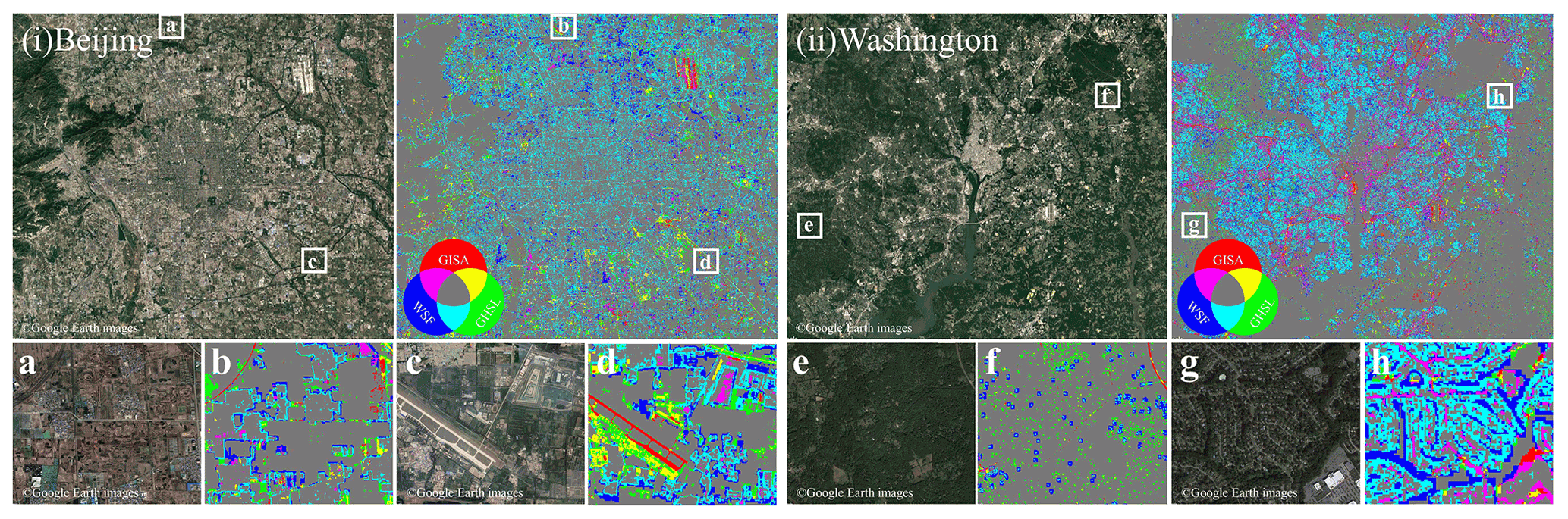
Figure 12 Illustration of WSF2015, GHSL 2018, and GISA-10m in (i) Beijing and (ii) Washington. Regions where the three datasets all agree are shown in gray.

5.2 Importance of multi-source features

In this study, we developed a global ISA mapping method that incorporates spectral, SAR, and temporal information extracted from multi-source Sentinel data. To illustrate the importance of multi-source features in global ISA mapping, we selected 30 hexagons in terms of the global urban ecoregions (Schneider et al., 2010). Urban ecoregions are defined with reference to biomes, urban landscapes, and economic levels. In each ecoregion, we randomly selected two grid cells with a population of greater or less than 5 million, respectively (Fig. S4). The “snow and ice” ecoregion was not considered. Feature contribution estimated by the RF classifier was employed to analyze the relative importance of the multi-source features (Pflugmacher et al., 2014). The different color schemes in Fig. 13 indicate the different types of features. For instance, the blue denotes SAR features while the green represents the spectral indices. The results indicate that the feature importance varies in the different regions. For example, SAR features are more effective in the temperate grassland of the Middle East and Asia (53N_75E and 50N_39E), while phenological features have more influence in the deciduous forest of Siberia (65N_125E). In particular, SAR features play a more important role in the more populated regions, e.g., in the temperate forest of North America and Europe and the temperate grassland of the Middle East and Asia (Fig. 13).

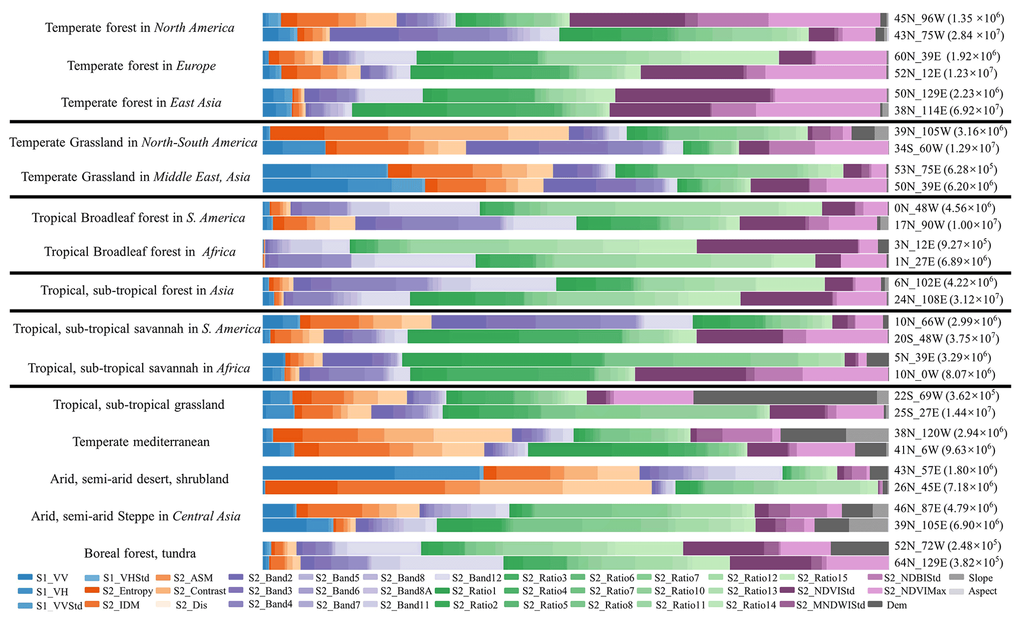
Figure 13 Relative importance of the multi-source features in 30 randomly selected grids located in different urban ecoregions. The labels on the right denote the grid ID and total population. Dis, IDM, and ASM represents the dissimilarity, angular second moment, and inverse difference moment, respectively.

It is worth noting that although high-rise ISA (e.g., buildings) tends to have higher radar backscatter, the importance of the SAR features is not always the highest. For example, in the hexagon of central US (45N_96W), the SAR features play a less significant role than the temporal metrics. In contrast, the spectral indices and phenological information are more effective in this region. For example, as shown in Fig. S5 (red squares), in the residential area, the buildings are often surrounded by dense shrubs, which can reduce the double bounce scattering. Therefore, the spectral and phenological features have a higher importance since they can better distinguish vegetation from non-vegetation. A similar situation occurs in a desert area (26N_45E) where the SAR features cannot distinguish ISA from NISA effectively due to the complex topography. In this case, the spectral indices and textures are more effective (Fig. 13). However, SAR features are still very important for global ISA mapping, especially for identifying rural buildings (Zhang et al., 2020). Therefore, in this study, we used multi-source features and hexagon-based adaptive RF models to ensure that the most suitable features were chosen for the different regions.

5.3 Impact of the training sample size and tree number

Based on the aforementioned randomly selected 30 hexagons in different urban ecoregions, we investigated the relationship between the training sample size and the accuracy (Fig. S4). For each hexagon, we fixed the number of NISA samples to 30 000, and changed the number of ISA_RS and ISA_OSM samples. Specifically, we first randomly selected 1000 ISA_RS, 1000 ISA_OSM, and 2,000 NISA samples from the candidate pool (see Sect. 3.1.1) as the test samples and used the remaining ones for the training. We randomly selected 50 ISA_RS and 50 ISA_OSM samples as the initial training samples and, subsequently, in an iterative manner, 400 ISA_RS and ISA_OSM samples were randomly selected from the pool and added to the training samples to train the RF classifier. It can be observed that all the hexagons reach saturation with 2500 ISA_RS and ISA_OSM samples (Fig. S6). Therefore, in this research, we set the number of ISA_RS, ISA_OSM, and NISA samples to 2500, 2500 and 30 000, respectively.

We also analyzed the effect of the tree number on the accuracy of global ISA mapping using the 30 aforementioned mapping grid cells from global urban ecological regions. The results show that the OA is low and unstable when the number of trees is less than 20 (Fig. S7). As the number of trees increases, the mapping accuracy increases and then stabilizes around 200 trees. Therefore, we used 200 trees for each RF model in GISA-10m.

5.4 Advantages of locally adaptive RF classification

We used two hexagons located in China (CHN) and Saudi Arabia (SA) to demonstrate the advantages of the adaptive RF classification. Although China and Saudi Arabia are both located in Asia, their urban landscapes and architectural styles are significantly different due to their differences in climate, environment, and culture. In this experiment, we migrated the training samples from one hexagon to classify the other one. For example, training samples collected in SA were used to classify the hexagon of China. The accuracy of each hexagon was evaluated by the visually interpreted samples inside it. The results show that the OA decreases by 34 % when the SA samples are applied to CHN (written as SA-to-CHN). Similarly, the OA is substantially reduced by 23 % by the transfer of CHN-to-SA. Furthermore, the local samples always outperform the migrated ones (see Table S7), which verifies the necessity of locally adaptive classification strategies in global ISA mapping. Furthermore, a locally adaptive model is more sensitive to the sample quality than a global model (Radoux et al., 2014), which further shows the necessity and effectiveness of the local classification strategy.

5.5 Influence of the sources of training samples

In this section, the effects of the training sample sources, i.e., the remote sensing dataset (ISA_RS) and the OSM database (ISA_OSM), were investigated. Various combinations of the ISA_RS and ISA_OSM training samples were tested at the global scale using the visually interpreted samples from Sect. 3.2 (Table S8). In general, it can be found that using both sources yields the most accurate results, which shows the effectiveness and necessity of incorporating training samples from both remote sensing and crowdsourced OSM data. By further checking the UA and PA of ISA, it can be seen that using both sample sources significantly improves the PA and reduces the ISA omissions, since the combination of ISA_RS and ISA_OSM strengthens the diversity of the training samples. Similarly, it is also found that the multi-source samples significantly raise the PA of NISA and lower its commission error.

Given that geographic bias in the spatial distribution of OSM data can affect the mapping results (Zacharopoulou et al., 2021), we applied temporal and spatial rules to mitigate the effect of the difference of the spatial distribution. In addition, a spectral rule was used to remove potential errors in the OSM-derived training samples (i.e., ISA_OSM). In fact, more than 82 % of the OSM ways are buildings and highways, whose total number exceeds 700 million (https://taginfo.openstreetmap.org/keys, last access: 20 June 2022). Therefore, OSM data provide a reference for large-scale ISA mapping, but have rarely been employed in global ISA mapping. We calculated the OA for the test grid cells where the number of ISA_OSM training samples was less than or larger than 2500 (i.e., the recommended size of training sample in Sect. 5.3). The results show that the accuracy of these regions is similar to the global accuracy (Table S9). This phenomenon demonstrates the stable performance of GISA-10m. Moreover, global ISA mapping using only ISA_OSM training samples shows a relatively stable accuracy across the continents (Fig. S8), suggesting that the refined OSM buildings and roads can reduce the impact of their uneven spatial distribution. This can be attributed to the rule-based method we implemented that improved the reliability and spatial consistency of ISA_OSM. In addition, the collaboration of ISA_OSM improves the OA of global ISA mapping by 3 % (Table S8), indicating the feasibility of OSM data in enhancing the performance of global ISA mapping after a series of refinements. Overall, although the spatial distribution of the OSM data is uneven, we tried to balance its spatial distribution through a series of rules, and incorporated multi-source geospatial data (e.g., satellite-derived datasets) to reduce the impact of geographical bias on GISA-10m.

6 Data availability

The GISA-10m dataset generated in this study is available in the public domain at https://doi.org/10.5281/zenodo.5791855 (Huang et al., 2021a). The Sentinel data were acquired from the GEE (available at http://code.earthengine.google.com, Google Earth Engine, 2021). The GHSL data were provided by the Joint Research Centre at the European Commission (available at https://ghsl.jrc.ec.europa.eu/datasets.php, GHSL, 2021). WSF was provided by the German Aerospace Center (https://doi.org/10.6084/m9.figshare.c.4712852, Marconcini et al., 2020b). The GlobeLand30 and GAUD were downloaded from the websites of the National Geomatics Center of China (available at http://www.globallandcover.com/, GlobeLand30, 2021) and Sun Yat-sen University (available at https://doi.org/10.6084/m9.figshare.11513178.v1, Huang, 2022). The FROM_GLC10, global urban boundaries, and GAIA were provided by Tsinghua University (available at http://data.ess.tsinghua.edu.cn, FROM-GLC, 2021). The GISA was provided by the Institute of Remote Sensing Information Processing at Wuhan University (available at https://doi.org/10.5281/zenodo.5136330, Huang et al., 2021c). The GLCFCS was provided by the Aerospace Information Research Institute at the Chinese Academy of Sciences (available at https://doi.org/10.5281/zenodo.4280923, Zhang et al., 2020). The Planet files were download from the OpenStreetMap website (available at https://planet.openstreetmap.org, OpenStreetMap, 2021).

7 Conclusions

In this study, we proposed a global ISA mapping method and produced a 10 m global ISA dataset (GISA-10m). To the best of our knowledge, this is the first global 10 m resolution ISA dataset based on Sentinel-1 and 2 data. To this end, a global training sample generation method was introduced based on a series of temporal, spatial, spectral, and geometrical rules, and 58 million training samples were generated from the existing global ISA datasets and VGI data (i.e., OSM). On the basis of the 2.7 million Sentinel images available on the GEE platform, multi-source features were constructed, including spectral, textural, SAR, and temporal metrics. The global terrestrial surface was divided with hexagons, and the results were obtained by a series of RF classifiers. In particular, the mapping was conducted adaptively for each hexagon by considering the difficulty and diversity for the global ISA detection. The OA of GISA-10m exceeded 86 % based on a set of independent test samples. The inter-comparison between the different global ISA datasets confirmed the superiority of the results obtained in this study. Based on the GISA-10m dataset, the ISA distribution at the global, continental, and country levels was investigated and compared. In addition, the global ISA distribution was compared between rural and urban areas. In particular, for the first time, courtesy of the high spatial resolution, the global road ISA was further identified, and its distribution was discussed.

The GISA-10m dataset could be used for global climate change studies and urban planning. The proposed rule-based sample generation method could also be applied for the global mapping of other land-cover categories. For example, the millions of cropland and forest tags in the OSM database could facilitate global high-resolution cropland and forest mapping. The ISA mapping method via multi-source geospatial data presented in this paper could also be improved by incorporating additional data sources, such as building footprints from Microsoft and Facebook (Corbane et al., 2021). In the future, we plan to extend the temporal coverage of GISA-10m and reveal the global ISA dynamics at the 10 m resolution.