Aridec: an open database of litter mass loss from aridlands worldwide with recommendations on suitable model applications

Plant litter decomposition in terrestrial ecosystems involves the physical and chemical breakdown of organic matter. Development of databases is a promising tool for achieving a predictive understanding of organic matter degradation at regional and global scales. In this paper, we present aridec, a comprehensive open database containing litter mass loss data from aridlands across the world. We describe in detail the structure of the database and discuss general patterns in the data. Then, we explore what are the most appropriate model structures to integrate with data on litter decomposition from the database by conducting a collinearity analysis. The database includes 184 entries from aridlands across the world, representing a wide range of climates. For the majority of the data gathered in aridec, it is possible to fit models of litter decomposition that consider initial organic matter as a homogenous reservoir (one pool models), as well as models with two distinct types of organic compounds that decompose at different speeds (two pool models). Moreover, these two carbon pools can either decompose without interaction (parallel models) or with matter transfer from a labile pool to a slowly decomposing pool after transformation (series models). Although most entries in the database can be used to fit these models, we suggest that potential users of this database test identifiability for each individual case as well as the number of degrees of freedom. Other model applications that are not discussed in this publication might also be suitable for use with this database. Lastly, we give some recommendations for future decomposition studies to be potentially added to this database. The extent of the information included in aridec in addition to its open-science approach makes it a great platform for future collaborative efforts in the field of aridland biogeochemistry. The aridec version 1.0.2 is archived and publicly available at https://doi.org/10.5281/zenodo.6600345 (Sarquis et al., 2022), and the database is managed under a version-controlled system and centrally stored in GitHub (https://github.com/AgustinSarquis/aridec, last access: 31 May 2022).

1 Introduction

Plant litter decomposition has a central role in the balance between carbon (C) storage and losses in terrestrial ecosystems. This process involves the physical and chemical breakdown of organic matter. Together with soil organic matter decomposition, this process is the main route of carbon dioxide (CO₂) efflux to the atmosphere in terrestrial ecosystems (Chapin et al., 2011). It also plays a key role in the formation and stabilization of soil organic carbon (SOC; Cotrufo et al., 2013). Therefore, in the context of current global change, a thorough understanding of decomposition is crucial for future C budget and storage predictions (Davidson and Janssens, 2006).

Arid ecosystems (hereafter aridlands) are variously defined as water-limited ecosystems, where the scarcity and unpredictability of precipitation drive most processes (Noy-Meir, 1973). They are also defined as regions where evaporation is higher than precipitation, which in turn limits ecosystem productivity (Jafari et al., 2018). Moreover, aridlands can be classified based on an aridity index as hyper arid, arid, semi-arid, and dry subhumid ecosystems (United Nations Environment Programme, 1997). Around 41 % of the global land area are considered as aridlands (Safriel and Adeel, 2005), and these systems are expanding due to global change (Feng and Fu, 2013; Reynolds et al., 2007; Yao et al., 2020). Despite their comparatively low productivity, some aridlands can have a potentially large impact on global CO₂ dynamics (Ahlström et al., 2015; Poulter et al., 2014). The wide extent of aridland cover and its influence on regional and global biogeochemical cycles make the study of aridlands a priority.

In particular, plant litter decomposition in aridlands is still not well understood (Austin, 2011). Litter mass loss in the field is mainly studied using the litterbag method or some variant (Harmon et al., 1999). The vast majority of litterbag studies come from temperate forests favored by the ease of litter collection and the concentration of researchers close to these study sites. There are fewer studies in aridlands, and few efforts have been made towards synthesizing aridland decomposition literature (Austin, 2011; Cepeda-Pizarro, 1993) or to examine patterns of decomposition in global aridlands (Zhang and Wang, 2015). Nonetheless, substantive literature has already been produced, which would allow for the compilation of a comprehensive database on plant litter decomposition in aridlands that could help boost our understanding of these ecosystems.

Development of databases is a promising tool for achieving a predictive understanding of organic matter degradation at regional and global scales (Luo et al., 2016). This predictive understanding can be obtained through mathematical models, but there is substantial uncertainty with respect to which models to use. For litter decomposition, some efforts have been made by fitting models with multiple C pools of different quality that decompose at different rates (Adair et al., 2008), as well as incorporating the effect of abiotic stressors like photodegradation on C dynamics (Adair et al., 2017; Chen et al., 2016; Foereid et al., 2011). Taken together, increased data availability and global representativity of well-constructed databases with our current most complex modeling tools could help us achieve a better understanding of the land C cycle with a higher predictive power.

Once a database of observations has been constructed, there exists the possibility of fitting complex models from these data, although this should be approached with caution. A common issue with mechanistic models used in environmental sciences is that they are poorly identifiable (Brun et al., 2001), meaning that different parameter sets of a model generate similar probability distributions for the observed data (Sierra et al., 2015). In other words, it is impossible to identify a unique set of parameters that explains model behavior. One reason behind this issue is that the information one would like to learn from models is often of a much higher complexity than the information content of the observed data (Brun et al., 2001). It is possible to detect identifiability issues by carrying out collinearity analyses (Sierra et al., 2015; Soetaert and Petzoldt, 2010), among other techniques. Thus, in addition to applying current ecological knowledge about underlying mechanistic processes in model construction, it is important to avoid identifiability problems when fitting these models with real data.

Another important aspect when developing this type of database is to follow an Open Science approach (Hampton et al., 2015). Open Science entails the practice of making all stages of scientific knowledge freely available and presented in a transparent and reproducible way for the whole scientific community to use. Such an approach has the potential to enhance the quality of research products and to speed up scientific progress through collaborative work. Particularly, the development of databases can benefit greatly from an open science perspective by allowing self-motivated reviewers to make comments and by allowing scientists from outside of the core research group to make their own contributions to the database, among other benefits. This latter aspect is key to ensure databases stay updated as new studies get published.

In this paper, we present aridec, a comprehensive open-science database that comprises time series of litter mass loss (decomposition) data from aridlands across the globe. First, we describe in detail the structure of the database and discuss general patterns in the data. Second, we run a collinearity analysis on the database to explore what might be the most appropriate model structures to fit. We chose a group of models of organic matter loss provided in the R package SoilR as potential models, including models of one, two, and three pools with and without matter transfers between them (Sierra et al., 2012). Third, we present an example of applied usage of the database. Lastly, we discuss the scope of the database and give outlines on good field decomposition experimental practices stemming from this work.

2 Methods

2.1 Database description

We conducted a Scopus search on 17 February 2021 for field decomposition studies of all times from aridlands published in peer-reviewed journals. We used the search words “arid” OR “dry season” AND “decomposition” and excluded results from unrelated subjects. This search produced a list of 1142 publications. To be included in the database, studies additionally needed to fulfill certain criteria: (a) field studies in which leaf, shoot or root litter of terrestrial plants was used, and (b) minimum of three time points of mass loss data. We did not include wood or dung decomposition studies. We also included publications from our personal libraries. In total, this left us with a list of 184 eligible publications.

We named the database aridec and uploaded it to a repository in GitHub (GitHub, 2022; Sarquis et al., 2022). From each publication selected, we created a database entry consisting of three separate files: a file containing time series of mass loss (timeSeries.csv), a file containing metadata of the study site and the experimental setup (metadata.yaml), and a file with relevant information of the initial characteristics of the litter at the beginning of the experiment (initConditions.csv). We saved each entry in an individual folder named after the last name of the first author and the year of publication. If there was more than one paper per author and year, we added lowercase letters to differentiate them (e.g., Austin2006a and Austin2006b). We included all entries inside the data folder. Other folders in the repository include the Rpkg folder containing an R package for querying and manipulating the database, a test folder with scripts for testing the integrity of the data and the R package, and an additional folder with miscellaneous scripts that demonstrate additional functionality. The overall structure of the database is similar to the structure of SIDb (Schädel et al., 2020), a database of soil incubation time series, and contains the following folder structure:

• –

  aridec

  • –

    Rpkg

  • –

    test

  • –

    scripts

  • –

    data

    • –

      single entry

      • –

        metadata.yaml

      • –

        initConditions.csv

      • –

        timeSeries.csv

The timeSeries.csv file includes litter mass loss over time as reported in the original publication. It is a csv type file (“comma-separated values”) with column names in the first row. The first column name is always the variable Time, and the first value in this column is always “0” (zero). Successive time values should be specified according to each sampling date reported in the study. Time units accepted are days, weeks, months, and years. Starting from the second column, column names should be unique variable identifiers. Below these names, mass loss data should be included as a percentage of the initial value, which is always 100. When data in the paper are reported in graph form, it is necessary to extract data point values with software tools such as WebPlotDigitizer (Rohatgi, 2020). Acceptable mass loss units are percentage of remaining dry weight, dry organic matter, dry ash-free mass, or C. For remaining mass data, as well as for time, units should be specified in the metadata.yaml file described below.

The metadata.yaml file includes additional information reported in the original paper. It is a yaml type file (“YAML ain't markup language”), which allows us to write lists of items in a hierarchical form and is both machine and human readable. It includes four main sections: entry identification data, the siteInfo, the experimentInfo, and the variables sections. A template for this file, with a full description of how to complete it, is available inside the data folder. The first part includes citationKey, which is a unique identifier for the whole entry in the format LastnameYEAR (lowercase letters must be added when there are two or more entries by the same author and year, i.e., LastnameYEARa and LastnameYEARb). This citationKey name should be the exact same as the folder name. Next is the doi, which stands for the digital object identifier where data is published. entryAuthor and contactName are both the first and last name of the person who wrote the entry file and their supervisor (only if applicable), respectively. If the entry author works independently of a supervisor, both fields should be filled with the same name. contactEmail should be filled with the supervisor's e-mail address. entryCreationDate stands for the date when the file was created, following the format: YYYY-MM-DD. entryNote should include any notes or comments related to this entry, such as missing data or additional data sources used to complete this file. Lastly, study requires a short study description of not more than one sentence.

The second part of the metadata.yaml file is the siteInfo section, which includes environmental information of ecological interest from the study site. First is the site field that requires an identification name for the site (not necessarily the site's real name). If the study includes more than one site, an array format should be used in this field, and the rest of the items in this section should be arrays of equal length. The coordinates field should be completed using decimal units, checking for the negative sign that denotes Southern and Western Hemispheres. If absent from the publication, coordinates can be approximately obtained from Google Earth (Google LLC, 2020). The country field should be completed avoiding full names (e.g., “China” instead of “People's Republic of China” or “USA” instead of “United States of America”). Mean annual temperature (^∘C) and mean annual precipitation (mm) should be entered in the fields MAT and MAP, respectively. When climatologic data are absent from the paper, they can be retrieved from other databases like the POWER database (NASA Langley Research Center, LaRC, 2021). The rainySeason field should be filled with either one of five options: whole year, spring, summer, autumn, winter; if precipitation does not follow a unimodal pattern, this item is left blank. Elevation of the study site in m a.s.l. should be entered under the elevation field, which if absent from the publication can be retrieved from other sources such as Google Earth. The type of vegetation cover of the site should be specified in landCover, with possible options: marsh, greenbelt, farmland, mangrove forest, subalpine, shrubland, urban, sandland, forest, steppe, desert, grassland, and savanna. The item vegNote should include a short description of not more than one sentence of the species or functional type composition at the site, if available. The cover item should be completed with percentage values of total plant cover or with cover values for specific plant functional types, as available. Lastly, the soilTaxonomy item must be completed using the taxonomic classification of the soil at the site. If the classification system used in the paper is unknown, it is better to leave this section blank, for exact equivalences between soil classification systems are unlikely.

The third part of the metadata.yaml file is the experimentInfo section, which includes information regarding the experimental design of the study. incDesc stands for incubation description and must include a short list of treatments and sampling points in time. The number of replicates should be specified, paying attention to occasional pseudo-replication in decomposition studies. The experiment duration in days should be completed with the maximum time length that samples stayed in the field. The month in which the experiment started should be specified under startingMonth. The name of the litter used for the experiment should be specified under litter, and it should match the name used in the initConditions.csv file (see below). Under the litterbag field, many sub-fields for different characteristics of interest should be completed, such as mesh material, mesh size (one side of a square in mm), dimensions (in cm), mesh transmittance (as a percentage of full sunlight), and litterbag position (full list of options available in the template file). A general rule for the experimentInfo section is that when there is more than one option for a field, they should be considered as different levels of a treatment. In this case, that field should be left blank in this section, and a new field should be created in the variables section by replacing the experimentalTreatment placeholder in each variable (see below).

The last section of the metadata.yaml file is the variables section, which serves as a link between columns in the timeSeries.csv file and metadata. Thus, this section should have as many variables as columns in the timeSeries.csv file. The first variable (V1) must always be called “Time” and only time units should be modified accordingly. The rest of the variables (V2 to Vn) must be adequately edited to represent treatment application as described in the original publication. Variable names should match column names in the timeSeries.csv file. Litter mass loss units should be expressed either in (dry) mass remaining, organic matter remaining, or C remaining. In our database, organic matter remaining is a synonym of ash-free dry mass remaining. This is because the ash-free dry mass correction assumes that ash is inorganic matter, and thus ash-free mass is equivalent to organic matter for the purpose of this database (Harmon et al., 1999). Under varDesc (as in variable description) one should write a brief sentence indicating specific treatment levels applied to this variable. The site field should be completed using the same site name entered in the siteInfo section. The experimentalTreatment item is a place holder for treatments with multiple levels. It should be replaced by any of the listed variables in experimentInfo and completed with an appropriate treatment level. In compTreat complementary treatments not included in the rest of the metadata items should be indicated using key words (e.g., grazed, ungrazed, water addition, control, etc.). Finally, transmittance and wavelength threshold (nm) data for radiation filters should be indicated under filter. This sub-section should be completed only for photodegradation studies.

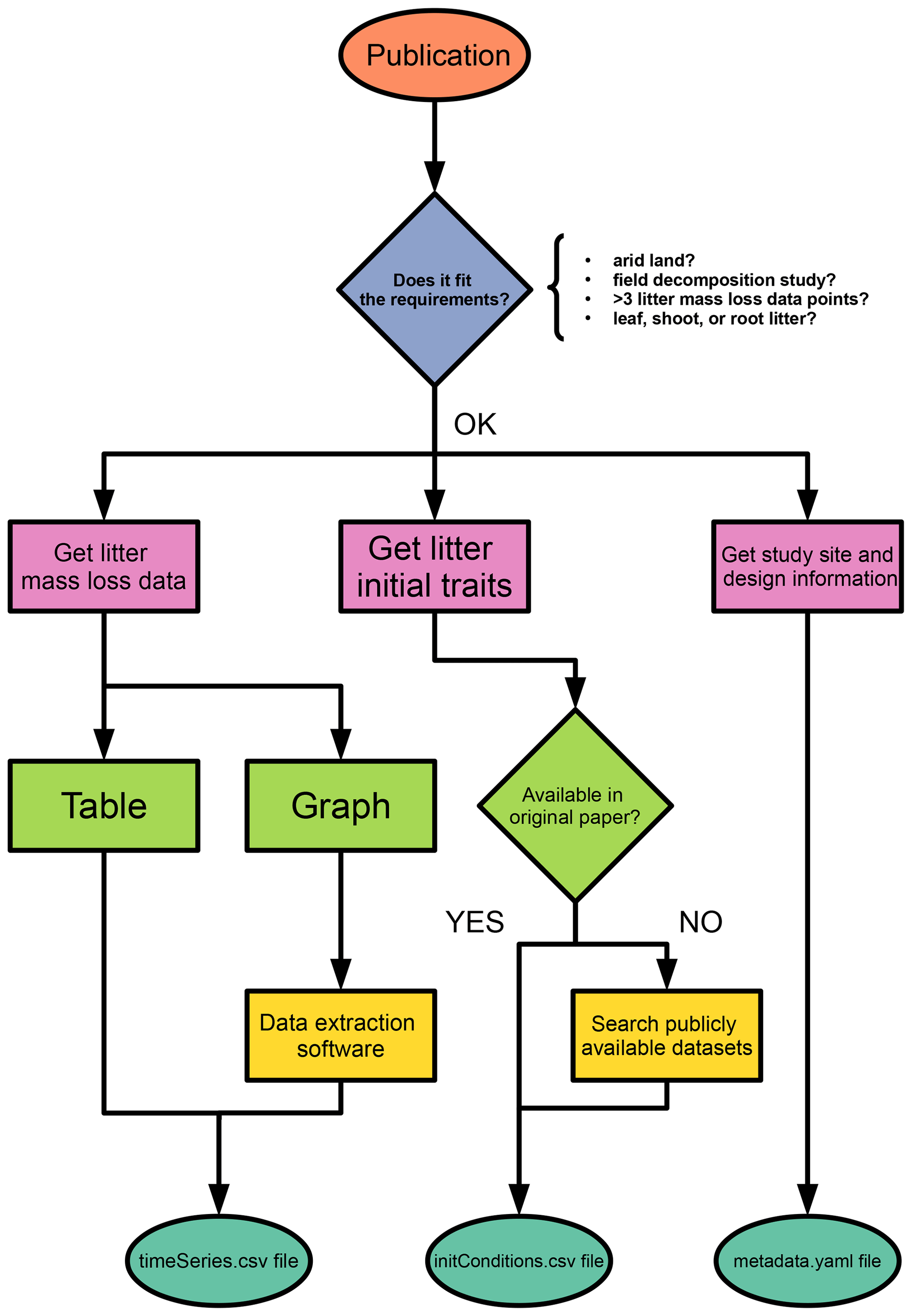
Figure 1 A guiding flowchart of the entry-submitting process for potential contributors of aridec.

The last file in the data folder is the initConditions.csv file, which contains details on the plant litter substrate used for each experiment. The first row contains column names. The first column name is species and is the only mandatory item; nonetheless we strongly recommend completing all items, if possible. We suggest checking for the correctness of scientific names in the Global Biodiversity Information Facility database (GBIF.org, 2022). Names in the species column should be used to complete the litter item in the metadata.yaml file. Four options are valid for the type column: deciduous or evergreen (for woody plants) and forb or graminoid (for herbaceous plants). For the N-fixer item, we recommend consulting the NodDB database (Tedersoo et al., 2018). Units for the sample amount column are in g, for the nutrients and fibers in percentage, and for SLA (specific leaf area) in mm² mg⁻¹. When litter quality traits are not provided in the original paper, they can be obtained upon request from the TRY database (Kattge et al., 2020). We created a template for the initConditions.csv and a README.md file with further instructions in the data folder. Special attention should be paid to the material section of the README.md file, for litter substrates are highly variable among studies, and this is key for database consistency. In Fig. 1, we present a flowchart with the full process of entry submitting for potential contributors.

We generated a global aridity index (GAI) map with the study sites from the database. We retrieved GAI data from the Consortium for Spatial Information global climate datasets (CGIAR-CSI; Trabucco and Zomer, 2019). This index is calculated after dividing the mean annual precipitation by the mean annual reference evapotranspiration. The raster dataset that we used is based on WorldClim2 database (Fick and Hijmans, 2017). We chose this dataset because it encompasses a relatively long period of time (from 1970 to 2000) and it has a high spatial resolution (∼1 km at the Equator). We then classified each study site by its GAI value as hyper-arid (0–0.05), arid (0.05–0.2), semi-arid (0.2–0.5), dry sub-humid (0.5–0.65), and humid (>0.65; United Nations Environment Programme, 1997). Complementarily, to explore how representative our sites in aridec are of the whole climatic range of aridlands, we first made a random point sampling of 6793 pixel units separated at least 1 km away from each other within the range of aridlands (GAI: 0–0.65). For each sample, we averaged mean monthly temperatures from WorldClim2 to obtain mean annual temperature values. We did the same for our aridec coordinates and plotted both sets of data together to evaluate how well aridlands are represented in our database. We used the QGIS software to process data and created a map (QGIS Development Team, 2021).

2.2 Model fitting and collinearity analysis

A central application of this database is the development of models of litter decomposition for aridlands. In an attempt to explore what the most appropriate model structures to integrate with data from the database are, we selected different structures of decomposition models based on recent theory of models of organic matter decomposition (Sierra and Müller, 2015). These model structures are already implemented in the SoilR package (Sierra et al., 2012), and we provide here an interface between our database and this R package. SoilR is a modeling framework that contains a wide set of functions and tools to model soil organic matter decomposition within the R computing platform (R Core Team, 2020).

Organic matter decomposition in SoilR is represented by systems of linear differential equations that generalize most compartment-based models. A simple general structure to represent litter decay with no inputs follows Eq. (1):

$$\begin{array}{}\text{(1)}& \begin{array}{rl}& {\displaystyle \frac{\mathrm{d}\mathit{C}\left(t\right)}{\mathrm{d}t}}=\mathbf{A}\mathit{C}\left(t\right),\\ & \mathit{C}\left(t\right)=[C_{\mathrm{pool}\mathrm{1}},\mathrm{\dots },C_{\mathrm{pool}m}{]}^T,\\ & \mathbf{A}=\left[\begin{array}{ccc}-k_{\mathrm{1}}& \mathrm{\cdots }& a_{\mathrm{1}i}\\ \mathrm{⋮}& \mathrm{\ddots }& \mathrm{⋮}\\ a_{j\mathrm{1}}& \mathrm{\cdots }& -k_m\end{array}\right],\end{array}\end{array}$$

where C(t) is a m×1 vector with m pools of litter mass observed at time t, and A is a square m×m matrix that contains decomposition rates (k_m) for each pool and transfer rates (a_ij) between them. These different pools may correspond to different ways in which the quality of the litter is expressed in different studies. For example, they may correspond to different compounds obtained from a specific extraction method (e.g., water soluble sugars or acid detergent lignin), or they can be defined by general decay classes such as fast and slow decay compounds. These pools have different decomposition rates, pool 1 being the fastest decomposing pool and pool m being the slowest. The linear dynamical system represented by Eq. (1) has many different solutions, but we are only interested in the solution that satisfies

$$\begin{array}{}\text{(2)}& C(t=\mathrm{0})={\mathit{C}}_{\mathrm{0}}=[\text{total }{\mathit{C}}_{\mathrm{0}}\cdot p_{\mathrm{1}},\mathrm{\dots },\text{ total }{\mathit{C}}_{\mathrm{0}}\cdot p_m{]}^T,\end{array}$$

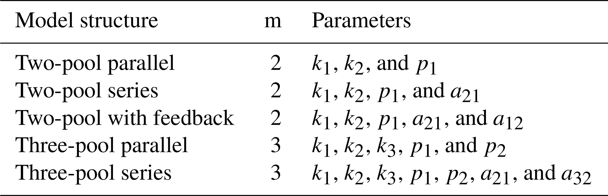
where C₀ is an m×1 vector with the value of initial litter mass content in the different compartments m. Total C₀ is set to be 100 % in SoilR for our database, and the resulting parameters p_m are the initial proportions of litter in m pools. Using this framework, we chose to fit a total of five different models with an increasing number of parameters (Table 1).

Table 1 Fitted model structures and parameters. m: number of C pools. k₁, k₂, k₃: decomposition rates of pools 1, 2, and 3, respectively. p₁, p₂: initial proportions of C in pools 1 and 2, respectively. a₂₁: transfer rate from pool 1 to pool 2. a₁₂: transfer rate from pool 2 to pool 1. a₃₂: transfer rate from pool 2 to pool 3.

For this set of models, we performed an identifiability analysis following the procedure described by Soetaert and Petzoldt (2010). Non-identifiability is a common issue with inverse-modeling approaches. It is a type of model over-parameterization that makes precisely determining parameter values virtually impossible; thus parameters are “non-identifiable”. When parameters are functionally related, changes in one parameter can be compensated by changes in others. This produces different parameter sets that have similar probability distributions, thus the inability to determine a single parameter set for the model (Sierra et al., 2015). Analyzing for parameter identifiability in models fitted with aridec data allowed us to assess which model structures are the most appropriate to use in this context.

This identifiability analysis is based on the calculation of the collinearity index (Brun et al., 2001). This index is a measure of the degree to which changes in one parameter are compensated by changes in other parameters for a certain model structure and dataset. We used the modCost function from the FME R package to first adjust a model cost function (Soetaert and Petzoldt, 2010). This function estimates weighted residuals of the model output versus the observed data and calculates sums of squared residuals, according to the formula:

$$\begin{array}{}\text{(3)}& {\text{res}}_{k,l}={\displaystyle \frac{{\text{Mod}}_{k,l}-{\text{Obs}}_{k,l}}{{\text{error}}_{k,l}\cdot n_l}},\end{array}$$

where Mod_k,l and Obs_k,l are the modeled and observed values for any data point, k, of a variable l, respectively. Error_k,l is a weighing factor that makes the term non-dimensional.

The model cost function, together with a set of pre-set initial parameter values, is then used as an input to calculate a matrix of sensitivity functions using the sensFun function from FME. This function estimates the sensitivity of the model output to the parameter values using the expression:

$$\begin{array}{}\text{(4)}& S_{ij}={\displaystyle \frac{\partial r_i}{\partial {\mathrm{\Theta }}_j}}\cdot {\displaystyle \frac{w_{{\mathrm{\Theta }}_j}}{w_{r_i}}},\end{array}$$

where S_i,j represents each entry of the matrix, r_i are model residuals calculated from the cost function, Θ_j is a model parameter, w_riis the scaling of r_i, and w_Θj is the scaling of parameter Θ_j (Soetaert and Petzoldt, 2010).

The final step in this analysis is calculating the collinearity index γ. The collin function from FME uses the sensitivity matrix as an input to calculate γ for every combination of parameters; γ is defined as

$$\begin{array}{}\text{(5)}& \mathit{\gamma }={\displaystyle \frac{\mathrm{1}}{\sqrt{min\left(\text{EV}\left[{\widehat{S}}^T\widehat{S}\right]\right)}}}.\end{array}$$

Here ${\widehat{S}}_{ij}$ is calculated as:

$$\begin{array}{}\text{(6)}& {\widehat{S}}_{ij}={\displaystyle \frac{S_{ij}}{\sqrt{{\mathrm{\Sigma }}_j{S}_{ij}^{\mathrm{2}}}}},\end{array}$$

where ${\widehat{S}}_{ij}$ contains the columns of the sensitivity matrix that correspond to the parameters included in the set, and EV estimates the eigenvalues. The collinearity index equals 1 if the columns are orthogonal, and the set is identifiable. The index equals infinity if columns in the sensitivity matrix are linearly dependent (Soetaert and Petzoldt, 2010). The interpretation of the collinearity index is thus a change in the residuals caused by a change in one of the parameters can be compensated by a proportional change $\mathrm{1}/\mathit{\gamma }$ in another parameter. For practical purposes, if γ>20, the parameter combination is considered non-identifiable (Sierra et al., 2015).

For the identifiability analysis, we first selected a representative group of 30 entries from the database ranging from three to 19 time points (Table 2). The number of data points in time limits the number of parameters that can be fitted because it affects the number of degrees of freedom. Thus, models with more parameters require longer datasets. This meant that, a priori, not all entries could be used to fit all model structures. On the other hand, it is possible to test identifiability for restricted model versions, that is, models with some of their parameters fixed to a known value. This implies that there are fewer parameters to be determined, and thus it allows us to use shorter time series. The details of all the models tested are reported in Table 3. From this first analysis, we noticed that two pool parallel and series structure models with a restricted initial proportion of litter in pool 1 (p₁) were the two models more likely to meet identifiability with our data. Because of this, we tested collinearity for all the 184 entries in the database, but only for these two models and for the respective models with the full set of parameters, for comparison. The R code for this analysis can be found in the collinearity.R script inside the scripts folder of aridec.

Table 2 Aridec entries used in the identifiability analysis with their corresponding DOI o URL. The number of time points refers to the number of sampling dates at each study plus the initial date.

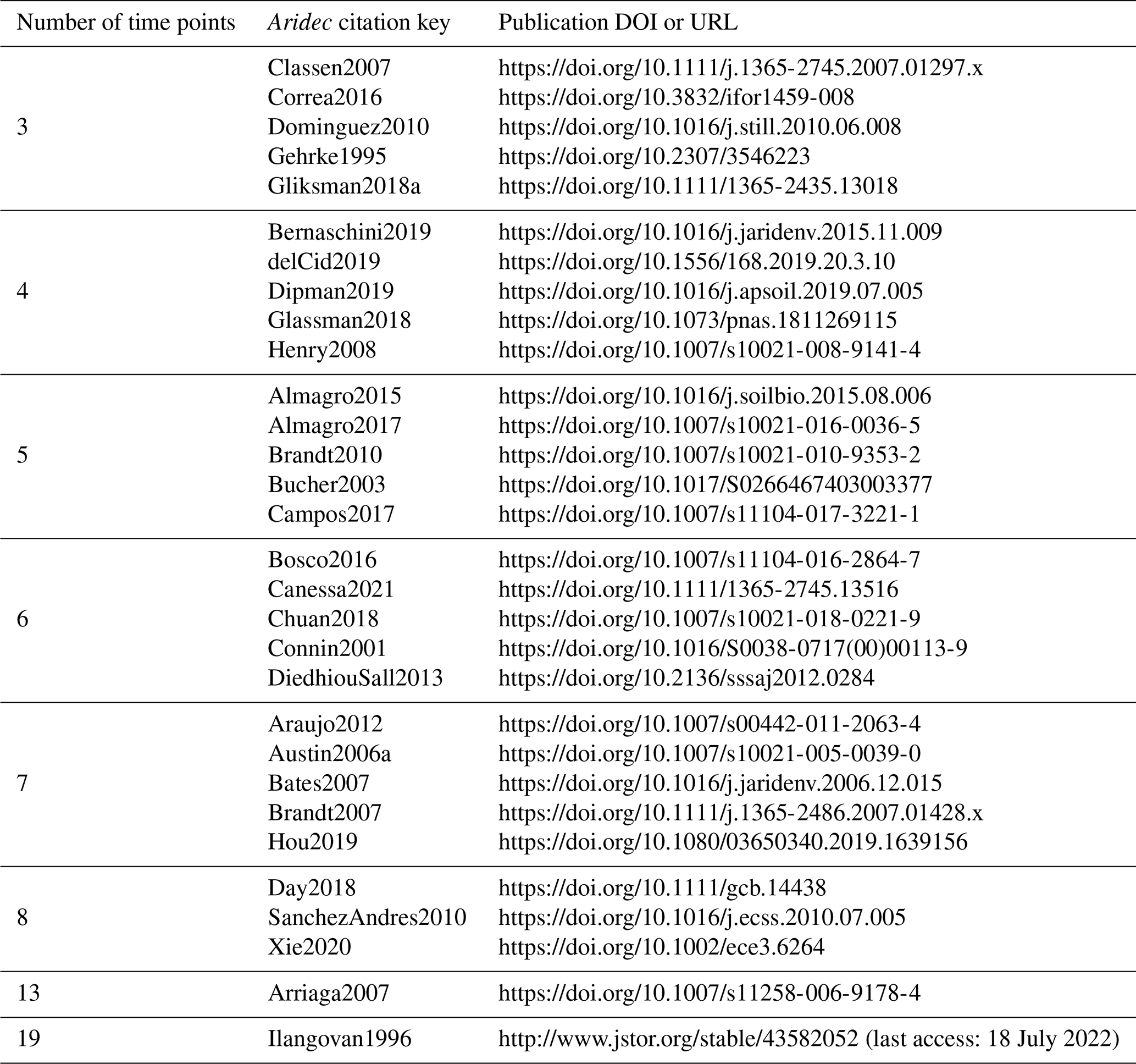
Table 3 Minimum number of time points in datasets fitted to each model structure T, number of parameters for each model structure P, number of datasets used for each model structure D, and the possible number of combinations of parameters to identify with specific combinations of available data C.

2.3 Applied example

Our collinearity analysis (see below) showed that although most entries could be used to fit two-pool parallel and series models with a fixed p₁ parameter (i.e., the initial proportion of litter in pool 1), this was dependent on each dataset. Restricting the p₁ parameter is a sensible way of achieving identifiability because it is common to find information on litter lignin content in decomposition publications, and this can be used as an initial proportion value for the slow-decomposing litter pool (i.e., p₂). Since

$$\begin{array}{}\text{(7)}& p_{\mathrm{1}}+p_{\mathrm{2}}=\mathrm{1},\end{array}$$

it is possible to estimate the p₁ as the complementary value of p₂.

To give a practical example of what can be done with this database, we chose to fit these models using one of the entries where both the models were identifiable, and the initial proportion of litter lignin was available. Together with these models, we fit a simple one-pool model for comparison. We used variable 2 (V2) from the Day2018 entry, which corresponds to Simmondsia chinensis (Link) C. K. Schneid. leaf litter decomposed under full sunlight treatment in the field (Day et al., 2018). The initial proportion of lignin (p₂) was 0.09. We used the Bias Corrected Akaike Information Criteria (AICc) to assess the model fit (Shumway and Stoffer, 2017).

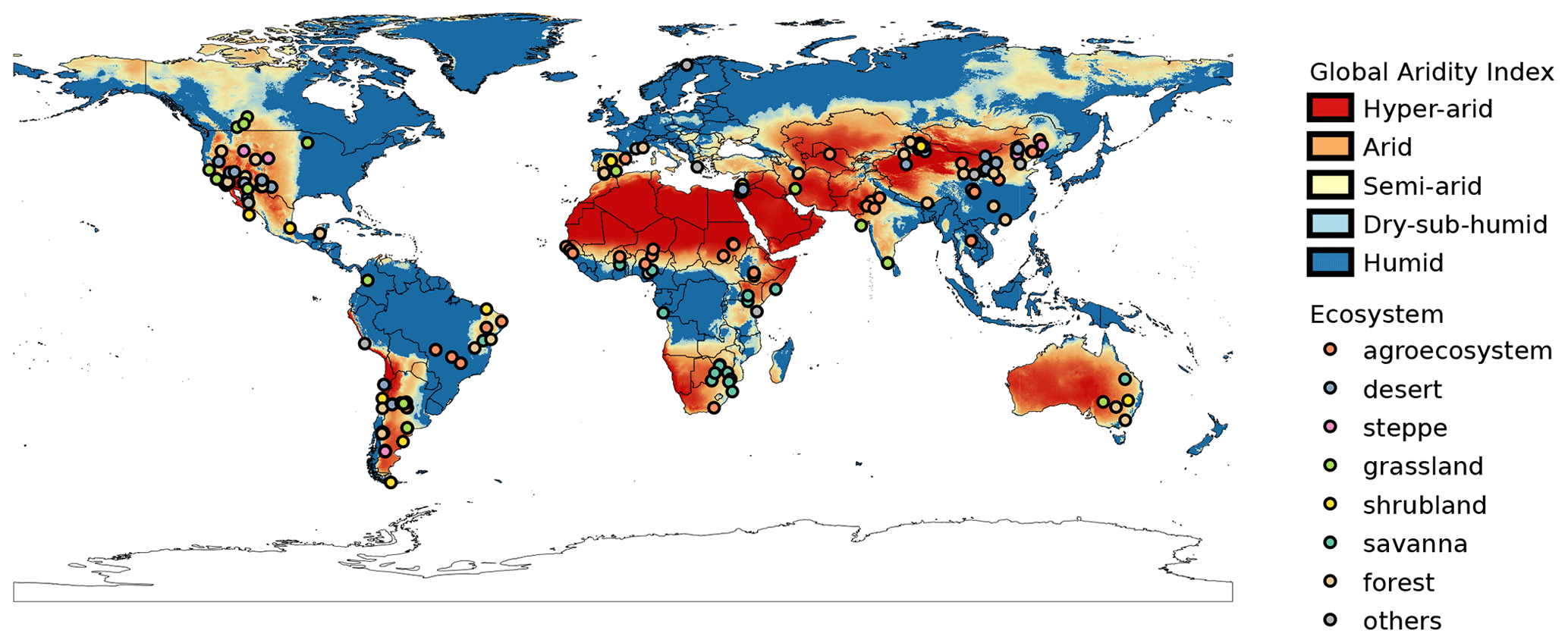
Figure 2 GAI map generated using data from the WorldClim 2 database. Hyper-arid: 0–0.03. Arid: 0.03–0.2. Semi-arid: 0.2–0.5. Dry sub-humid: 0.5–0.65. Humid: >0.65. Points represent study sites in the aridec database. Colors represent different ecosystems as reported in the original publications.

3 Results

3.1 Data overview

The 184 studies in the database included data for 212 unique study sites around the world. Twenty-four of these sites were repeated in two or more studies. According to the GAI, ∼3.6 % of sites were classified as hyper-arid (0–0.05), ∼35.9 % as arid (0.05–0.2), ∼43 % as semi-arid (0.2–0.5), ∼6 % as dry sub-humid (0.5–0.65), and ∼12 % as humid (>0.65). We recognize that humid sites do not classify as aridlands, but we included them nonetheless because these sites had marked dry seasons according to the original publications. A total of 33 countries was represented in our database. The top-five countries with the largest number of study sites were China (58 sites), USA (49 sites), Argentina (32 sites), Israel (22 sites), and Brazil (12 sites). Most sites in the database correspond to arid regions where the mean annual temperatures are above zero degrees Celsius, with a very low representativity of colder regions (Fig. 3)

Out of the 184 database entries, we retrieved 1752 series of litter mass loss over time. The oldest publication in the database is from 1975, and the newest is from 2021. Moreover, there has been a considerable growth in the number of publications per year (Fig. 4a). The study duration in the database ranged from 18 d to 10 years, with a median of 365 and a mean of 430 d (Fig. 4b). The number of sample harvests from the field went from 2 to 23, with a mean of ∼6 and a median of 5 (Fig. 4c). The sampling frequency ranged from 0.08 to 11.1 samples per month, with a median of 0.4 and a mean of 0.8 samples per month (Fig. 3d). Elevation at the study sites varied from −375 to 4000 m a.s.l., with median and mean values of 557 and ∼811 m a.s.l., respectively (Fig. 4e). The mean annual temperatures ranged from −0.45 to 29.5 ^∘C at the study sites with a mean value of 14.9 ^∘C and median of 15.6 ^∘C (Fig. 4f). The mean annual precipitation in aridec ranged from 2 to 1700 mm, with median and mean values of ∼375 and ∼494 mm, respectively (Fig. 4g). Out of all sites, 23 % were reported by the authors to be deserts, 17 % forests, 16 % agroecosystems, 12 % grasslands, 10 % shrublands, 10 % steppes, 8 % savannas, 2 % coastal ecosystems, and 2 % urban sites (Fig. 4h).

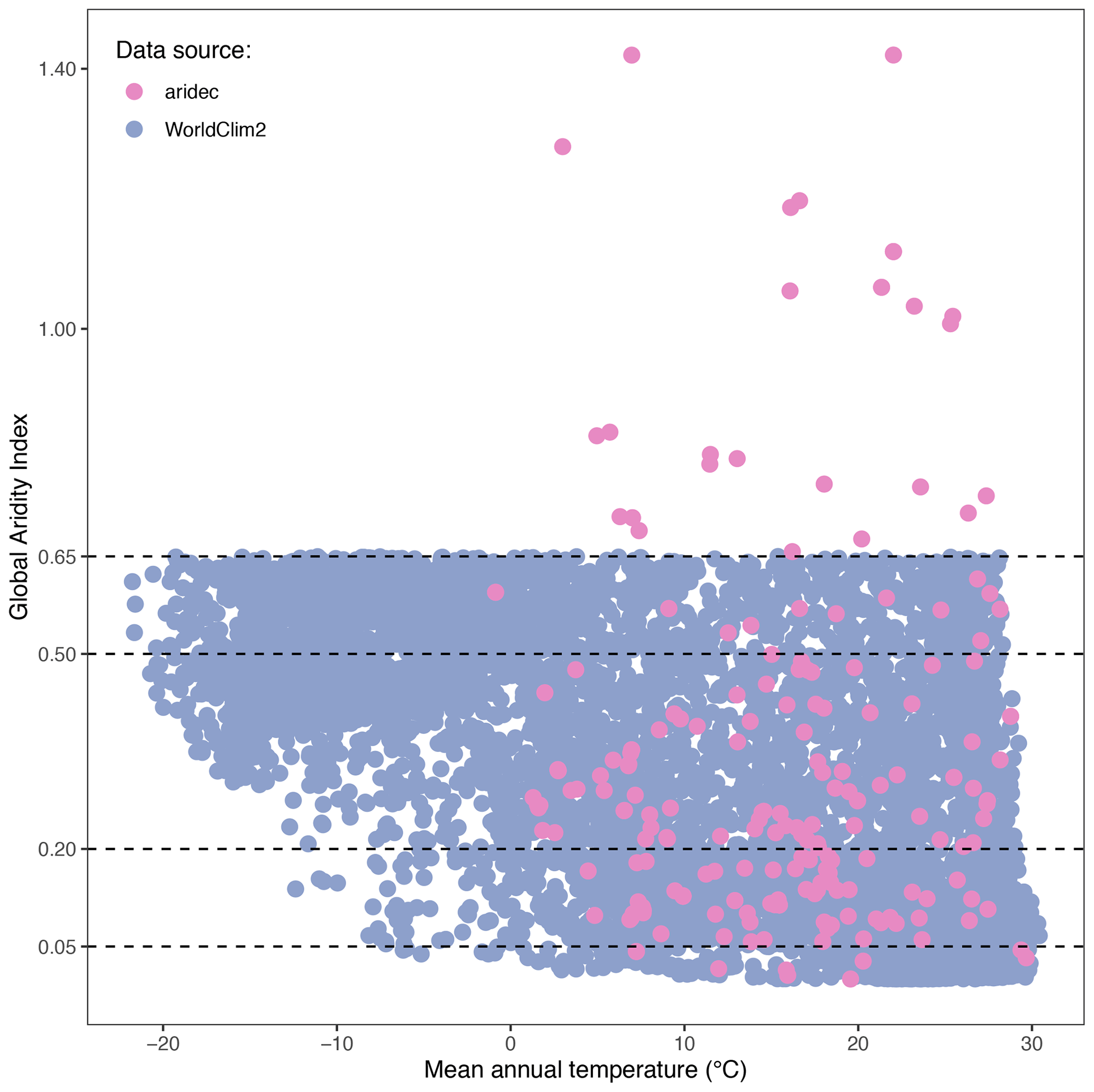
Figure 3 Climate representativity of the aridec database. GAI plotted against mean annual temperature (^∘C). WorldClim2 points were generated via a random sampling of 6793 pixels in QGIS. All data comes from the WorldClim2 database. Horizontal dashed lines represent the breaks in GAI between aridland categories: hyper-arid, 0–0.03; arid, 0.03–0.2; semi-arid, 0.2–0.5; dry sub-humid, 0.5–0.65; humid, >0.65.

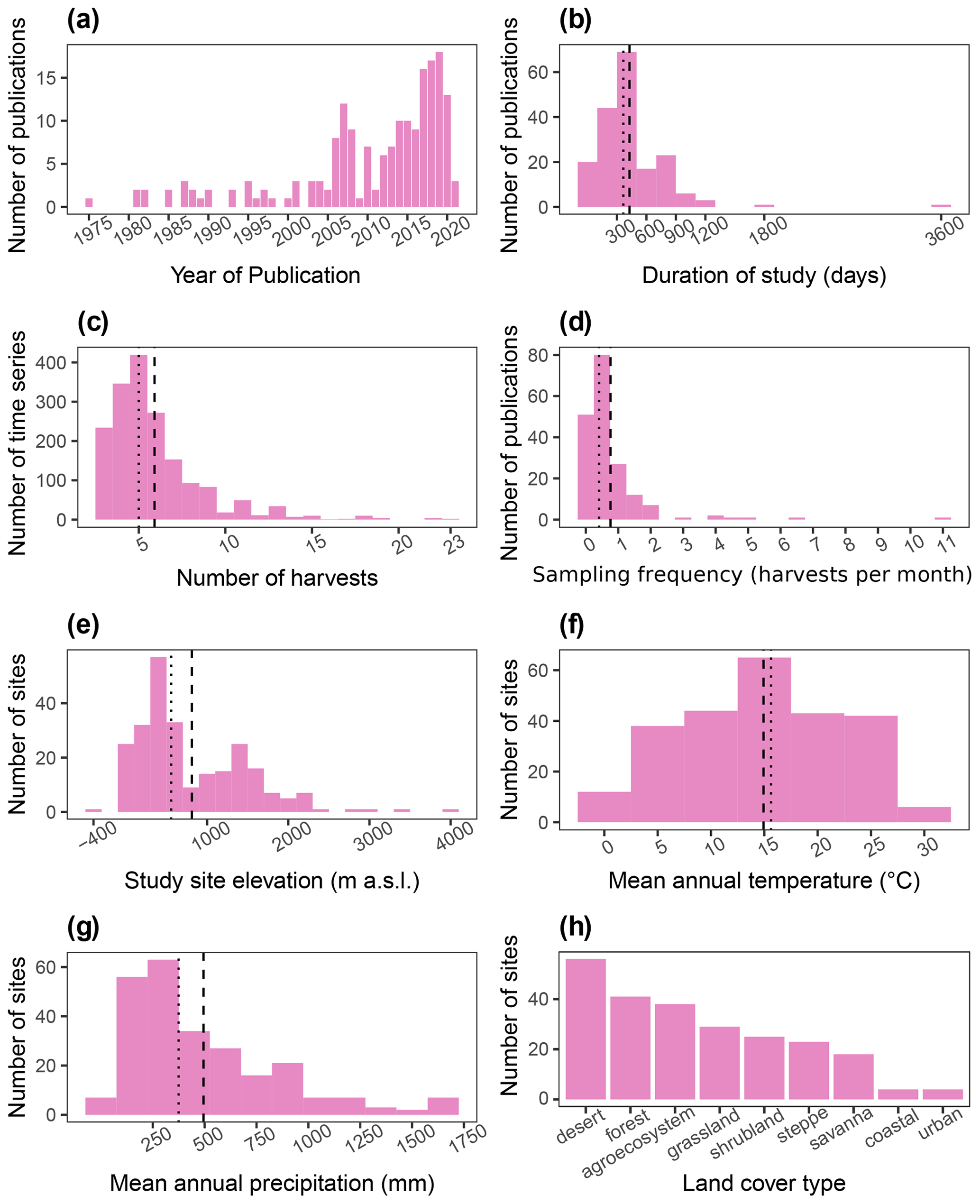
Figure 4 Aridec data overview including number of publications per year (a), study duration in days (b), number of sample harvests (c), study sampling frequency as number of samplings per month (d), study site altitude in m a.s.l. (e), mean annual temperature in ^∘C (f), mean annual precipitation in mm (g), and number of studies per type of land cover (h). Dashed lines represent the mean, and dotted lines represent the median in each panel.

3.2 Identifiability analysis

Figure 5 shows results from the first identifiability analysis carried out on a subset of 30 entries. Here, we can compare how entries with an equal number of time points behave under each model structure. For the two-pool parallel model structure, four parameter combinations were compared: a full three-parameter model and three alternative models with one restricted parameter each. There were 30 points for the full model with 62.1 % of values below the collinearity index γ=20 threshold, i.e., almost 40 % of the models were not identifiable. For the models restricted to two parameters, 95.6 % out of the 90 models compared were identifiable. When specifically looking at the model with a restricted p₁ value, 100 % of the models were identifiable. This was expected because usually the fewer the parameters to be estimated, the lower the collinearity in models.

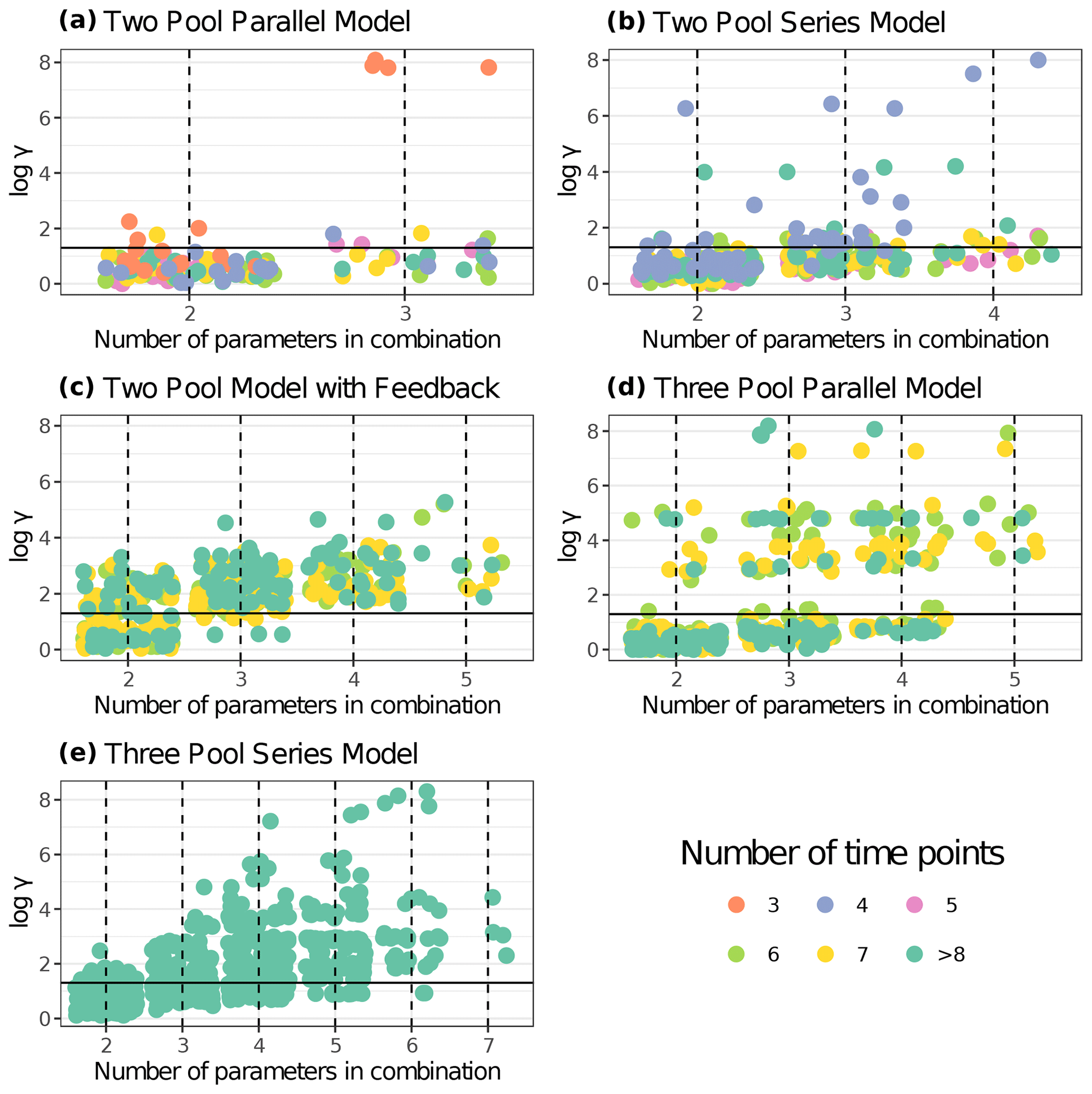
Figure 5 Collinearity index (γ) comparison for different model structures using entries from aridec. γ values were log₁₀ transformed, and horizontal lines at log₁₀(20) denote the maximum value of γ for a model to be considered identifiable. Infinite γ values were not plotted. Each panel shows data for a different model structure. The number of entries from the database used for each model structure is reported in Table 3. Each point represents γ for a model structure fitted for a specific dataset with different parameter combinations. The color scale for data points shows the number of data points in each dataset (i.e., the number of sampling dates plus the initial date). Values with >8 time points were grouped for easier interpretation. The number of model variants fitted for each model structure and database entry were n=30 for the two pool parallel model with all three parameters and n=90 with one restricted parameter (a); n=25 for the two pool series model with all four parameters, n=150 with two restricted parameters, and n=100 with one restricted parameter (b); n=15 for the two-pool model with feedback and all five parameters, n=150 with two and three restricted parameters, and n=75 with one restricted parameter (c); n=15 for the three pool parallel model with all five parameters, n=150 with two and three restricted parameters, and n=75 with one restricted parameter (d); n=5 for the three pool series model with all seven parameters, n=250 with five restricted parameters, n=300 with four restricted parameters, n=230 with three restricted parameters, n=115 with two restricted parameters, and n=35 with one restricted parameter (e).

The two-pool series model structure analysis included a full four-parameter model and ten alternative models with one or two restricted parameters each. From a total of 25 full parameter models, 48 % were identifiable according to their γ values. Out of 150 models with two restricted parameters, 94.7 % of models were identifiable, while for models with only one restricted parameter, 68.3 % of models were identifiable. When specifically checking for the collinearity index in models with a restricted p₁ parameter, 84.6 % of them were identifiable. The non-identifiable values in this last case corresponded to four entries with four time points each. That means that 100 % of models with >5 time points were identifiable for the restricted p₁ model version. This highlights the importance of having longer time series available for modeling.

The case of the two-pool model structure with feedback included a full parameter model and 24 other model variants with one, two, and three restricted parameters each. The analysis of 15 models with all five parameters showed 100 % of non-identifiable results. The results for the restricted model version with four parameters showed 100 % of non-identifiable models out of 75 data points, while only 4.7 % of the 150 data points with three parameters gave γ values lower than 20. The analysis of the restricted model version with two estimated parameters generated 57.3 % of identifiable results out of 150 models.

When testing for the three-pool parallel model structure, we used one full model with five parameters and 24 model variations comprising from two to four parameters each. None of the full model data points showed collinearity index values lower than 20. Out of the restricted four-parameter models only 34.7 % could be identifiable. When we specifically looked at the models where either p₁ or p₂ were fixed, none of them were identifiable. Restricted models with three parameters produced a 68 % of identifiable results. Further, restricted models that only had k values were not identifiable. Finally, 89.3 % of models restricted to two parameters were identifiable according to our analysis.

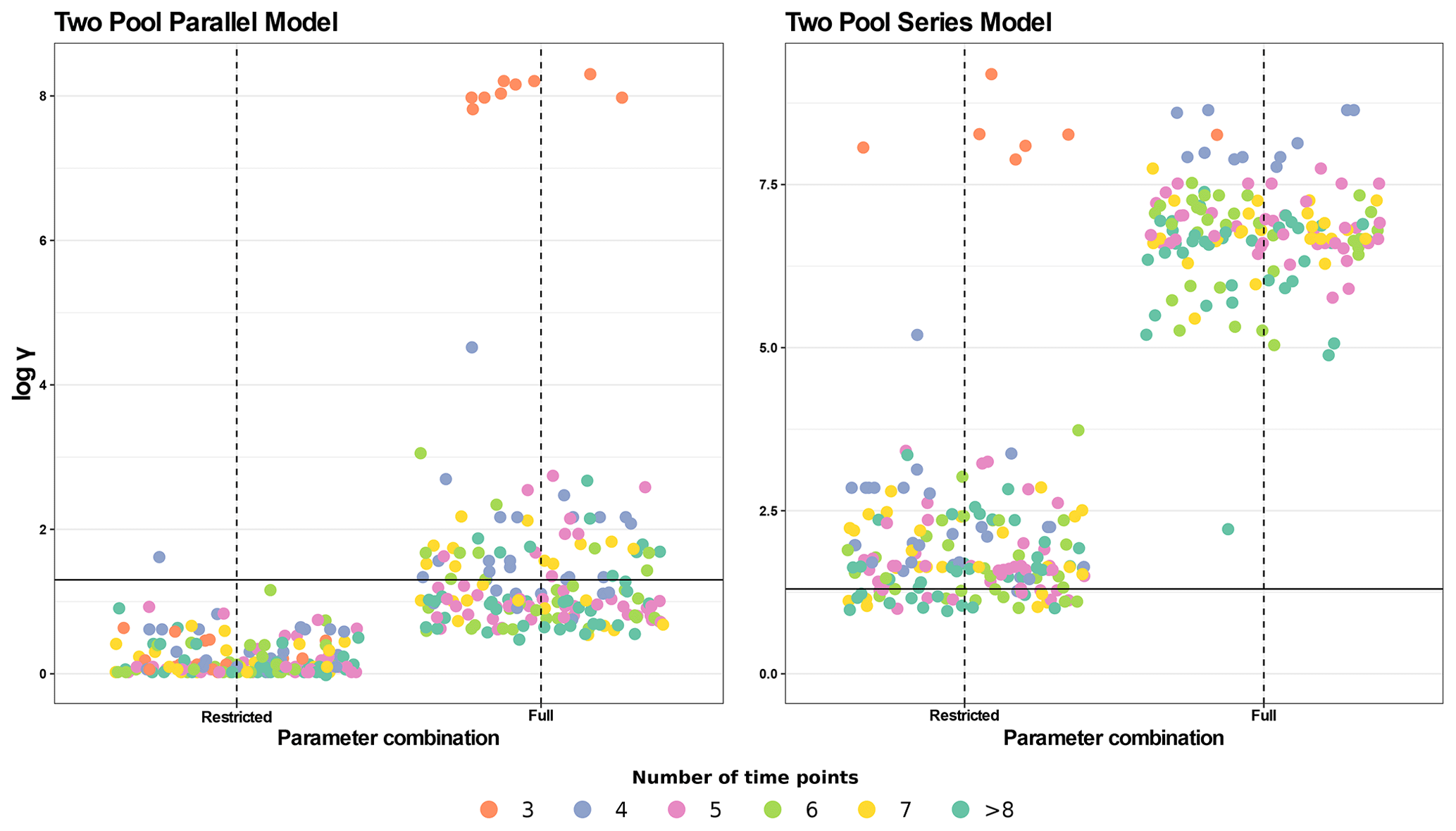
Figure 6 Collinearity index (γ) comparison for four different model structures using the entire database. The full parameter combination includes k₁, k₂, p₁, and a₁₂ (the latter only for the series model). The restricted parameter combination excludes p₁. γ values were log₁₀ transformed and horizontal lines at log₁₀(20) denote the maximum value of γ for a model to be considered identifiable. Infinite γ values were not plotted. Each panel shows data for a different model structure. Each point represents γ for a model structure fitted for a specific dataset with different parameter combinations (n=184, for each model structure). The color scale for data points shows the number of data points in each dataset (i.e., the number of sampling dates plus the initial date). Values with >8 time points were grouped for easier interpretation.

The last model structure analyzed was the three-pool series structure, which produced comparisons for models with all seven parameters, plus 118 other model variants with different restricted parameters. None of the models with all seven parameters were identifiable. Only 5.7 % of the models with six parameters were identifiable, none of which corresponded to the models where either p₁ or p₂ were fixed. Models restricted to five parameters produced 10.5 % of identifiable results. Specifically looking at models with both fixed p₁ and p₂, 100 % of those were not identifiable. Restricting models to four parameters generated 28 % of results with γ>20. Models with three estimated parameters produced 54.9 % of identifiable results. Lastly, 84.8 % of models restricted to only two parameters were identifiable.

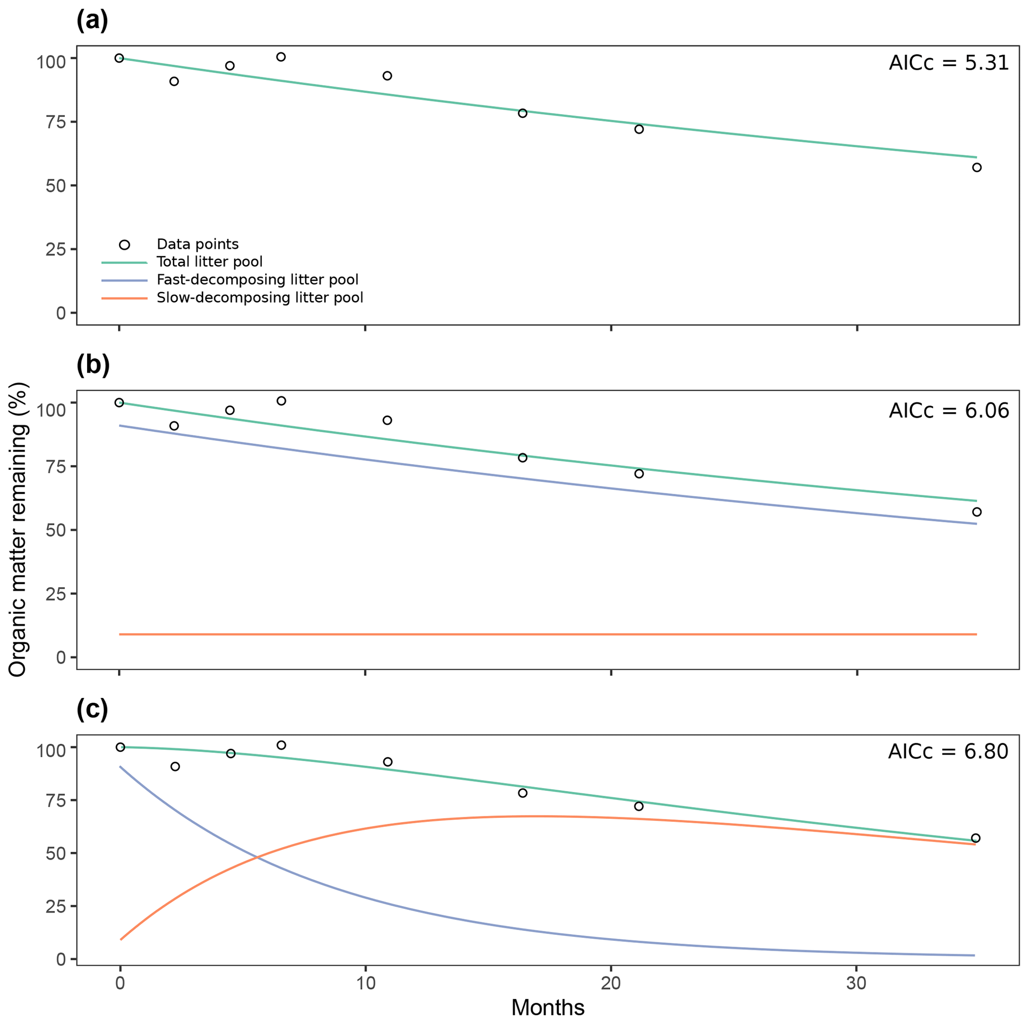
Figure 7 Comparison of three different decomposition model structures fitted with time series of organic matter loss from the Day2018 entry: one-pool model (a), two-pool model with a parallel structure (b), two-pool model with a series structure (c). AICc: Akaike Information Criteria, Bias Corrected.

Because two-pool parallel and series models with a fixed p₁ parameter showed the highest percentage of identifiable cases in this first analysis, we did a second test with the whole database for these models and for their respective full-parameter versions for comparison (Fig. 6). For the two-pool parallel model with the full set of parameters, 58.7 % of entries were identifiable, whereas restricting the p₁ parameter yielded 99.5 % of identifiable entries. For the more complex series models, the percentages of identifiable entries were much lower, with only 20.1 % for the restricted version and no identifiable cases for the version with a full set of parameters. Clearly, restricting the number of parameters to be estimated decreases collinearity, but the results are highly variable and dependent on each particular dataset.

3.3 Applied example

The previous analysis of the collinearity index (Fig. 6) shows that from the proposed model structures to be fitted, our data can, in most cases, be fitted to two pool parallel and series structure models with a restricted initial proportion of litter in pool 1, aside from single-pool models. Figure 7 shows the results from the simulation of the dynamics of organic matter loss from leaf litter fitted from the Day2018 entry. The one-pool model showed how a single reservoir of organic matter from leaf litter decomposed at a k rate of 0.0142 per month (Fig. 7a). At the end of the almost 3-year period, the remaining percentage of total organic matter was 61.02 %. The two-pool parallel model showed a fast decomposing organic matter pool with a k₁ of 0.0158 per month (Fig. 7b). This pool went from representing 91 % of total organic matter to 52.4 % after almost 3 years. On the other hand, the slow decomposing pool, which we defined as the initial lignin content of litter, had a value of k₂ of $\mathrm{1.5}\times {\mathrm{10}}^{-\mathrm{16}}$ per month. We defined this pool as 9 %, and it remained unchanged after 2 years, which was expected from a k₂ of nearly zero. Lastly, the two-pool series model showed a fast decomposing pool with a k₁ of 0.11 per month (Fig. 7c). This pool went from 91 % of total organic matter to 1.7 % at the end of the experiment. In this case, the slow decomposing pool had a k₂ of 0.02 per month. This model also had a transfer coefficient from the fast decomposing pool to the slow pool of 1 (i.e., 100 % of organic matter in the fast pool that decomposed in a month transformed into more recalcitrant forms, adding to the slow decomposing pool). Then, the slow decomposing pool went from 9 % at the start of the simulation to 54.08 % after almost 3 years. Judging by their AICc values, the three models were similarly supported by the data.

4 Discussion

4.1 The aridec database

The aridec database is a comprehensive database with a wide range of information on decomposition studies from aridlands worldwide, which includes litter mass loss data, litter traits, and experimental design information. Our exhaustive bibliographic search gave us close to 200 papers that fulfilled our criteria. Notably, we did not limit our work to studies published in English; aridec also includes papers in Spanish, Portuguese, and Mandarin. This widens the scope of our work to achieve a more inclusive database.

From a geographic perspective, study sites included in aridec cover most of the main aridlands of the world (Fig. 2). As expected, countries like China, USA, and Argentina had the largest number of studies, which might be related to the extension of aridlands in these countries, since China has 6.07×10⁶ km² of drylands (Huang et al., 2019), and around 40 % and 69 % of USA and Argentina territories are considered as drylands, respectively (Verbist et al., 2010; White and Nackoney, 2003). In contrast, some of the biggest deserts in the world, such as the Sahara, the Kalahari, the Australian Outback, and the Arabian desert are underrepresented, if not absent, in our database. Future efforts should focus on this information void, and the aridec database will be available to include these coming studies in our framework.

Study sites in the database represent a big part of the climate range where aridlands occur, from hyper arid deserts to dry sub-humid ecosystems (Fig. 2). Some of the study sites (∼12 %) were classified as humid according to the GAI. We chose to include them because those studies reported marked dry seasons at the study sites and focused on seasonal patterns of litter decomposition. The range of climatic variables such as mean annual temperature and precipitation, physical variables like altitude, along with land cover types are also very well represented in this database (Fig. 4). This wide representativity of climates in aridec is a crucial asset if the database is to be used to answer global-scale questions. Nonetheless, dry sub-humid lands but mainly hyper-arid deserts are the least represented in the database, suggesting more studies should be developed in these areas. Moreover, there is a void in the colder end of the climatic range of aridlands (Fig. 3). This might be related to the lack of sites in aridec of ecosystems like tundra where the GAI is mostly low, but a bibliographical search like ours could not retrieve the studies in those areas. There is clearly much room to expand our database and increase its potential applications.

One of the advantages of the aridec database is that its files are compatible with R and, specifically, with the SoilR library (Sierra et al., 2012). In addition to the fact that this database is an open-source and open-code project, there is huge potential for broadening the extent of the information in aridec and for developing code to work with it. Nonetheless, we should mention that the formats included in the database are not R-exclusive and can be used with most commonly available software. YAML files can be read and edited from any text processor, and CSV files can also be opened with any spreadsheet software. Although statistical analysis on R scripts cannot be used elsewhere, raw data itself can be freely processed with any statistical software.

The aridec database can be used on its own, but we recommend complementing our information with other publicly available databases to expand the application possibilities. Metadata are not always fully reported in publications, so it is possible to fill these gaps with climate and altitude data from databases like NASA Prediction of Worldwide Energy Resources (POWER; NASA Langley Research Center (LaRC)). Leaf litter traits are a big part of the database and are sometimes poorly reported in publications. A general source of litter traits data can be obtained upon request from the TRY database (Kattge et al., 2020). Another more specific source of information is NODdb, where nodulating-N-fixing plant genera are detailed (Tedersoo et al., 2018).

4.2 Model fitting within aridec

Based on our collinearity analyses (Figs. 5 and 6), we suggest that before fitting any models to our data, it is crucial to check the identifiability of the parameters with each database entry. We assume that all entries can be fitted to a one-pool model, since there is only one parameter to estimate. As for the more complex models, the situation is highly dependent on which data entry is being used. For instance, although most entries could be used to fit two-pool models with parallel and series structures, there are some exceptions. Another example can be seen in Fig. 5b, where one dataset of more than eight points was not identifiable for a model with all four parameters. Besides collinearity, the number of degrees of freedom will restrict which models can be fitted to the data so that these two aspects should be considered together. As models get more complex, we had to progressively exclude entries with less time points because they did not have enough degrees of freedom. As a concluding remark, the results in Figs. 5 and 6 are not to be interpreted as how those models perform in general but how they perform with the specific data in aridec. That is why we provide an R script in the database to test collinearity for individual datasets.

Moreover, in most cases, fitting these models is only possible by restricting the parameters estimated to only decomposition constants and transfer coefficients. We suggest restricting models to these parameters because it is more likely to find data on initial proportion of lignin or cellulose to be used as proxies for parameters p₁ or p₂. Not only might they be more difficult to find in the literature but estimating values for decomposition constants and transfer coefficients might altogether be a better use of this database. Further, we recognize that for some specific combinations of parameters and datasets, the more complex models might be identifiable (data points below the log₁₀(γ=20); Fig. 5).

Again, interconnection between datasets like aridec and others like TRY (Kattge et al., 2020) is a key workaround to the collinearity problem by providing data for parameter restriction (Sierra et al., 2015). We recognize that limitations in data available from field studies ultimately restrict our capability to fit more complex models (Brun et al., 2001). This limitation can have further implications if we consider the proportion of identifiable datasets per ecosystem type or level of aridity. For example, semi-arid and dry sub-humid ecosystems show the lowest proportion of identifiable datasets for a two-pool parallel model with all parameters (data not shown). This would lead to an under-representation of some aridlands because of a lack of suitable data available. Moving forward, new decomposition studies should consider making more measurements and including data on litter initial chemical quality, as well as expanding studies to less represented climates and ecosystems. This will allow for the detection and modeling of finer scaled dynamics of organic matter (see Appendix A).

The applied example in Fig. 7 serves as a glimpse of the potential of this database. Choosing which model to fit with decomposition data is not a minor task. For instance, none of the three models were supported as the best model from their AICc, which suggests that they must all be considered when making conclusions from this simulation (Anderson and Burnham, 2004). Whether a time series has a better fit with one model or another depends mostly on mass loss dynamics that were captured by the experimental design. While longer datasets can generally be fitted with more complex models, if the overall mass loss dynamics fit better for a one-pool model, higher model complexity will not be chosen using AIC. It is also to be considered that ecological theory may come into play here instead of applying purely statistical reasoning. As was pointed out recently, litter decomposition is not as much a process of “what is lost” but more of “what is left” (Prescott and Vesterdal, 2021). A balance between statistical fit and theoretical support should be found when choosing which model is best for each study case.

The aridec database is available for open access and download at http://github.com/AgustinSarquis/aridec (last access: 31 May 2022; Sarquis et al., 2022). Our hope is that newer studies on dryland litter decomposition will be added to the database by new collaborators (see Appendix A). It is important to follow our user guidelines to ensure consistency, all of which are available in the database itself. File templates for uploading new entries to the database are given, and further details can be found in them. Additionally, users will find in the database a README file, scripts to test file consistency and many examples on how to apply functions and to fit models using R code.

To our knowledge, the aridec database is unique. Other databases that focus on land C studies include the Soil Incubation Database (SIDb; Schädel et al., 2020), a peatland productivity and decomposition parameter database compiled by Natural Resources Canada (Bona et al., 2018), and the Chilean Soil Organic Carbon Database (CHLSOC; Pfeiffer et al., 2020). Although they all intend to assess questions related to C budgets in terrestrial ecosystems to some extent, not all of them present decomposition data (i.e., Pfeiffer et al., 2020). Moreover, only SIDb (Schädel et al., 2020) and aridec contain time series of organic matter loss. This is a unique asset that allows for future studies to make new assessments of decomposition without having to worry about inconsistencies in the calculation of k parameters. Finally, none of these other databases are centered around plant litter decomposition in aridlands like aridec.

The extent of the information included in aridec in addition to its open-science approach makes it a great platform for future collaborative efforts in the field of aridland biogeochemistry. In this sense, the main purpose of this database is to further our understanding of C dynamics at the earth system level. Complete datasets like aridec are necessary to test which model structures and parameters best explain decomposition processes and to help develop more realistic representations of the global C cycle in drylands (Luo et al., 2016). Further, additional parameters could be used to test the importance of mechanisms that are relevant in aridlands but are under-represented in the literature. Studies on processes like photodegradation (Adair et al., 2017) could be expanded to a wider geographical range and to soil processes thanks to the representation of sites in aridec using the SoilR framework (Sierra et al., 2012). Another potential application of our database is to combine ecological data with climatic data in earth system models, which is a promising framework to assess future global change stresses and their effects on the biosphere (Bonan and Doney, 2018).

5 Code availability

All scripts necessary to obtain figures in this publication are included in the database inside the “scripts” folder.

6 Data availability

Version 1.0.2 of aridec is publicly available at https://doi.org/10.5281/zenodo.6600345 (Sarquis et al., 2022). Documentation of the project and the R package are presented on the project's website (https://github.com/AgustinSarquis/aridec, last access: 31 May 2022). The database is open for reuse, and the usage license follows the GPL-3 license (https://opensource.org/licenses/GPL-3.0, last access: 9 February 2022). When using the database or R package, users should cite this definition publication and consider citing individual studies (publication or dataset).

7 Conclusions

The aridec database is a comprehensive database with a wide range of information on decomposition studies from aridlands worldwide. Study sites included in aridec cover most of the main aridlands of the world and represent well the range of climatic conditions that characterize aridlands. We found that although many studies have been conducted in aridlands, there is low representativity in cold arid regions, where new studies should be performed to obtain a more comprehensive understanding of decomposition in aridlands worldwide.

Our identifiability analysis showed that the information content in litter decomposition studies can only inform simple models with one or two pools. More complex models can be obtained for datasets with multiple data points, and a well characterized initial litter mass quality (such as lignin or cellulose content), which will result in low collinearity index values and allow for enough degrees of freedom.

One of the best assets of the aridec database is that its files are compatible with R and the SoilR package, making collaborative work more direct and approachable. Although our application suggestions are based on the use of the SoilR package, we recognize that other approaches might be suitable for the use of this database.

To our knowledge, the aridec database is unique, and the extent of the information included here in addition to its open-science approach makes it a great platform for future collaborative efforts in the field of aridland biogeochemistry.

Appendix A: Recommendations for future decomposition field studies

Compiling published studies for the database led us to come up with a set of recommendations that scientists working on field decomposition studies may take into consideration in order to incorporate future entries in aridec.

• Coordinates: from the database, 7.6 % of entries had errors in their site coordinates, and 8.7 % had no coordinates at all. This means that for 16.3 % of entries, we had to either look for coordinates in other publications or search for the approximate location on Google Earth. Exact coordinates are a must for a study to be incorporated in geospatially explicit databases. Since nearly half of the problematic entries corresponded to typographic errors, we recommend that authors and reviewers check for the correctness of coordinates. Further, we suggest providing coordinates as exact as possible and to avoid using vaguely broad coordinates (e.g., reporting coordinates of the closest town to the study site).

• Soil classification: out of all entries only 29.3 % reported soil taxonomy from the study site correctly. An additional 7.1 % of entries provided a classification for the soil, but they did not specify the classification system they used (i.e., FAO, WRB, or USDA). This is important because names of soil taxa are not always exclusive to a single classification system, and their definitions are most unlikely interchangeable (Hughes et al., 2017). For most studies this information might not be available, but for those where it is, we suggest reporting it. Otherwise, making inference from soil types would be impossible.

• Mesh transmittance: only 13.6 % of entries in aridec had measured the light transmittance of the mesh that they used to construct litter bags. Light interception by mesh can be very high: as much as 50 % of total radiation, photosynthetically active radiation, or ultra-violet radiation, as seen in our database. Considering the established importance of sunlight as a decomposition driver in aridland ecosystems (Austin et al., 2016), studies with mesh materials that block a significant proportion of light might be inducing unwanted effects and underestimating effects of photodegradation. We recommend, if possible, choosing high-transmittance materials (the highest in our database has 95 % transmittance of total radiation), measuring mesh transmittance and reporting these values in the corresponding publication.

• Sampling dates: the matter of choosing when to pick up samples from the field is complex. Ideally, the total amount of sampling dates and the amount of time between those dates should only depend on the hypothesis. The reality is that logistics has a huge impact on what scientists do, especially for field ecological studies. How researchers chose to set their sampling dates will determine the scale of the patterns that they will be able to detect from their experiments. For example, in some aridlands, where decomposition is very slow, litter might take years to fully decompose, and short experiments are not able to capture this part of the process. Most of the studies in aridec lasted around a year, with only a few studies lasting longer (Fig. 4b). Further, in some systems, leaching can have a big impact during the first days to weeks of decomposition, and more frequent sampling at the beginning of the experiment may allow us to detect this. In our database, most studies made measurements less than once a month (Fig. 4d), meaning that only monthly to yearly processes could be detected. These limitations extrapolate to modeling challenges; it is not possible to fit data to models that represent patterns that went undetected due to the study design. To accurately estimate decomposition rates (k) it is thought that litter at the last sampling date needs to have lost at least 50 % of mass. As such, this suggests that the number of samplings and extension in time of the study should reflect these goals. We suggest that researchers be aware of all these issues and also that they have enough pickups to actually be able to calculate the slopes of the relationships, which increases the power of inference enormously.

• Corrections of mass loss measurements: after collection from the field, in most cases, samples carry with them moisture and inorganic matter from the site. This can, of course, underestimate measurements of litter mass loss. Once in the laboratory, samples should be cleaned of any extraneous material and their moisture content measured. After this, a portion of each sample should be used to quantify the proportion of ashes (Harmon et al., 1999). This should also be done for samples that were not taken to the field and are used for measurements of initial litter traits. All mass loss analysis should be done on an oven-dried, ash-free basis.

• Time series: a large number of studies could not be included in aridec because they only published decomposition rates. As much as this is common practice, it limits the possibilities for incorporation into databases like ours and further analysis that might need temporal dynamics data as input. We suggest not only providing averaged values of mass loss over time, but also raw data as supplemental material. This helps bridge the reproducibility gap in ecological studies and represents a step forward to an open-science approach (Hampton et al., 2015).

• Initial litter quality: the characterization of litter chemical and physical traits at the beginning of experiments is an important tool for answering research-specific questions of decomposition studies. However, from our results, it was evident that these initial litter traits are also useful to decrease model collinearity (Fig. 6). Particularly, the initial content of litter components that constitute a big part of total mass like cellulose, acid detergent lignin, or water-soluble sugars can be used as proxies for the initial proportion of litter mass in pools of different decomposition rates. Unfortunately, not even half of the studies in aridec reported initial lignin content for each litter type. We managed to complete up to 48 % of lignin content data by averaging across database entries of the same species and by requesting data from TRY database. To our surprise, we only found lignin values for three out of the 236 litter types that we searched in the TRY database. This leads us to suggest that not only should authors measure and report these characteristics of interest, but they should also contribute their data to open-access databases from which other scientists can benefit.