A high-resolution inland surface water body dataset for the tundra and boreal forests of North America

Inland surface waters are abundant in the tundra and boreal forests of North America, essential to environments and human societies but vulnerable to climate changes. These high-latitude water bodies differ greatly in their morphological and topological characteristics related to the formation, type, and vulnerability. In this paper, we present a water body dataset for the North American high latitudes (WBD-NAHL). Nearly 6.5 million water bodies were identified, with approximately 6 million (∼90 %) of them smaller than 0.1 km². The dataset provides area and morphological attributes for every water body. During this study, we developed an automated approach for detecting surface water extent and identifying water bodies in the 10 m resolution Sentinel-2 multispectral satellite data to enhance the capability of delineating small water bodies and their morphological attributes. The approach was applied to the Sentinel-2 data acquired in 2019 to produce the water body dataset for the entire tundra and boreal forests in North America. The dataset provided a more complete representation of the region than existing regional datasets for North America, e.g., Permafrost Region Pond and Lake (PeRL). The total accuracy of the detected water extent by the WBD-NAHL dataset was 96.36 % through comparison to interpreted data for locations randomly sampled across the region. Compared to the 30 m or coarser-resolution water datasets, e.g., JRC GSW yearly water history, HydroLakes, and Global Lakes and Wetlands Database (GLWD), the WBD-NAHL provided an improved ability on delineating water bodies and reported higher accuracies in the size, number, and perimeter attributes of water body by comparing to PeRL and interpreted regional dataset. This dataset is available from the National Tibetan Plateau/Third Pole Environment Data Center (TPDC; http://data.tpdc.ac.cn, last access: 6 June 2022): https://doi.org/10.11888/Hydro.tpdc.271021 (Feng and Sui, 2020).

1 Introduction

Inland surface waters include various types of water bodies, including rivers and streams, large and small lakes, reservoirs, and ephemeral ponds. Inland surface water occupies only 2 % of the global land surface (Pekel et al., 2016), but it plays a critical role in terrestrial ecosystems. Surface water distribution varies across the landscape. More than 55 % of global surface waters are located in high latitudes in the Northern Hemisphere (>44^∘ N), and these northern high-latitude waters are generally small and densely clustered. The high latitudes have warmed faster than other regions, with annual surface temperatures increasing >1.4 ^∘C over the past century (IPCC, 2014). The temperature of the Arctic, in particular, has risen twice as fast as the average global temperature (Graversen et al., 2008; Johannessen et al., 2004; IPCC, 2007; Serreze and Francis, 2006; Li et al., 2020). This change in climate is driving changes in terrestrial ecosystems in the Arctic as well. For example, increases in vegetation productivity have been observed across the northern high latitudes (Forkel et al., 2016). Meanwhile, high-latitude water bodies have started changing since the early 1970s (Carroll et al., 2011; Carroll and Loboda, 2017; Cooley et al., 2019; Smith et al., 2005; Fayne et al., 2020; Nitze et al., 2020). Although some changes are seasonal, and therefore temporary, permanent changes have been reported, and small lakes in permafrost regions are found to be more vulnerable to permanent changes in water extent (Carroll and Loboda, 2017; Karlsson et al., 2014).

With observed rising temperatures (Biskaborn et al., 2019), permafrost thawing poses a threat to the stability of inland surface waters, especially in arctic lowland surface areas, where most of the water bodies could be thermokarst lakes (Jones et al., 2011; Olefeldt et al., 2016) and have strong interactions with permafrost in the regions. Thawing permafrost not only leads to the formation of lakes and ponds of various sizes, but also leads to the release of organic carbon in the form of carbon dioxide (CO₂) and methane (CH₄) (Serikova et al., 2019). Changes in lake formation may result in concomitant changes to the extent and connectivity of surface water bodies, which can greatly impact the sustainability of aquatic ecosystems.

The morphology of the water bodies could be shaped by the surrounding environment (Grosse et al., 2013; Laird et al., 2003; Schilder et al., 2013; Sharma et al., 2019; Carpenter, 1983; Higgins et al., 2021). Shoreline complexity affects lake ice formation (Sharma et al., 2019). Lake connectivity affects fish migration (Laske et al., 2019; McCullough et al., 2019), fish habitats, aquatic assemblages (Napiórkowski et al., 2019; Jiang et al., 2021), and water self-purification and accelerates water cycling (Glińska-Lewczuk, 2009; Vaideliene and Michailov, 2008; Xiong et al., 2017). The density of water bodies impacts fish density and biomass (Sandlund et al., 2016; van Zyll de Jong et al., 2017; King et al., 2021). The shape and distribution of water bodies reflect what led to the water body formation (Smith et al., 2007). Furthermore, information about lake area extent can improve Arctic land surface modeling (Langer et al., 2016; van Huissteden et al., 2011). For these reasons, it is critical to quantify high-latitude surface water extent, as well as characterize related morphological and topological features, including size and shape.

In the past, inland surface water was mapped at sub-hectare (i.e., 30 m) resolution using satellite data (Feng et al., 2015; Pekel et al., 2016; Pickens et al., 2020), and these data provided unprecedented information about the global extent of inland waters, including their spatial distribution and temporal changes. These datasets provide data that delineate the extent of large and moderate sizes of water bodies but underrepresent or fail to include the large number of small water bodies. Coarse-resolution datasets also lead to underrepresentation in delineating complex shorelines and the shapes of surface water bodies, making it difficult to derive their morphological and topological attributes. Existing datasets containing information that describe water body shapes, such as the Global Lakes and Wetlands Database (GLWD) (Lehner and Döll, 2004) and HydroLAKES (Messager et al., 2016) are limited to water bodies larger than 0.1 km². In spite of these limitations, these datasets provide valuable information for improving the precision of mapping inland waters. Detecting the extent of inland surface water at finer spatial scale boosts our ability to map small water bodies and improves the precision of delineating the shorelines of water bodies. This analysis then allows us to derive an inventory dataset of water bodies along with their morphological and topological attributes. The information allows scientists to analyze a water body as an object instead of a cluster of pixels, advancing our analysis and understanding of the water bodies' size, shoreline complexity, ecological effects, hydrological function, and vulnerability to natural and anthropogenic changes.

In this paper, we present a higher-resolution water body dataset for the North American high latitudes (WBD-NAHL). The dataset was derived by identifying the extent of inland waters using 10 m resolution Sentinel-2 multispectral data. The dataset provides the spatial extent and morphological attributes for each identified water body. It is the first inland water inventory dataset derived at this landscape scale with the capability of delineating inland surface waters as small as 0.001 km².

2 Spatial extent

The WBD-NAHL dataset covers all tundra and boreal forest biomes in North America (Fig. 1), with the exception of the Arctic Archipelago and Baffin Island due to their long time of snow or ice covering over water bodies. The topography of the tundra and boreal forest in North America is extremely diverse, varying from mountains and rolling hills to plateaus and flat coastal plains. The mountains of the North American Cordillera are covered by numerous mountain glaciers and also a large number of glacial lakes. A large number of thermokarst lakes were found in lowland tundra areas, e.g., the Yukon Delta and the Alaska North Slope (Olefeldt et al., 2016). The vast Canadian Shield also has a high density of lakes. The climate of this study region is characterized by long, cold winters and short, cool summers. The plants in the northern tundra include lichen, moss, grass, sedge, and shrub. The southern boreal forest is dominated by evergreen forests (Ritter, 2006). Lakes are widely distributed in the study region, and approximately 36 % of the land surface is covered by water (Messager et al., 2016). The number of lakes in this region accounts for 50 % of the global lakes, and the area of lakes accounts for 30 % of the global lakes in the region, indicating the region to be one of the richest areas of surface water bodies (Messager et al., 2016). Various types of lakes, including organic, fluvial, meteorite, volcanogenic, and anthropogenic lakes, are distributed in the study region and feature very different sizes and shapes (Dranga et al., 2017).

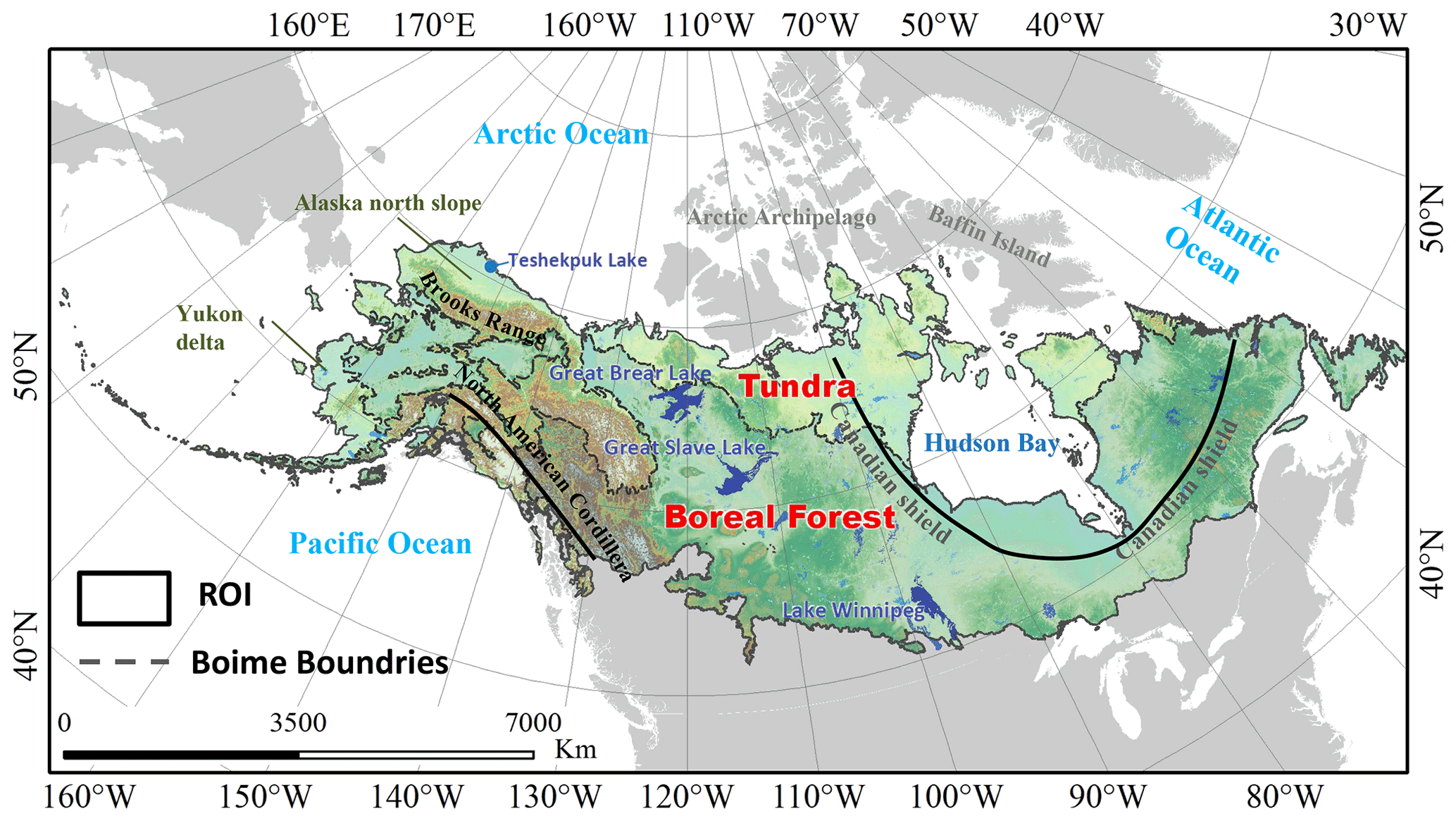
Figure 1 The extent of the study area, including the tundra and boreal biomes, in the North Americas continent, excluding the Arctic Archipelago and Baffin Island.

3 Data

3.1 Sentinel-2 A and B multi-spectral images

Sentinel-2 multi-spectral images were used to delineate surface water bodies in this study. Sentinel-2 A and B provide a short revisit cycle (2–3 d) in the high latitudes, which is critical for detecting surface water during the short, snow-free season in the region. Sentinel-2 images were obtained using the United States Geological Survey (USGS) EarthExplorer client–server interface (https://earthexplorer.usgs.gov/, last access: 7 April 2021).

Each Sentinel-2 image consists of 13 multispectral bands, including four bands at 10 m resolution, six bands at 20 m resolution, and three others at 60 m resolution. Sentinel-2 data are distributed as collections representing different processing levels. We selected the Sentinel-2 Collection 2 data, which provides spectral bands of surface reflectance after atmospheric corrections. The 10 m Sentinel-2 bands were used for water detection to maximize spatial precision for delineating small water bodies. The 20 m Sentinel-2 bands were resampled to 10 m resolution to match the higher-resolution bands. The “s2cloudless” (https://github.com/sentinel-hub/sentinel2-cloud-detector, last access: 7 April 2021) was applied to identify cloud-contaminated pixels, generating a probability of cloud and cirrus detection. This module includes a model generated by a convolutional neural network (CNN) trained with 6.4 million manually labeled samples. This model was validated to have 99 % accuracy for identifying clouds and 84 % accuracy for identifying cirrus in Sentinel-2 images (Zupanc, 2020).

3.2 Joint Research Centre (JRC) yearly water dataset

The JRC yearly water dataset (JRC GSW Yearly Water Classification History, v1.2, https://global-surface-water.appspot.com/, last access: 19 December 2020) (Pekel et al., 2016) provides a delineation of permanent water, non-water, and seasonal water for global inland surface waters. The dataset was produced using long-term Landsat images, including Landsat TM, ETM+, and OLI images acquired from 1984 to 2019. Permanent water in the dataset was identified as water cover throughout the entire year, and seasonal water is identified based on occurrence during a single year.

The JRC yearly water dataset provides a reasonably accurate delineation of water distribution for the period 1984–2019, but its precision is limited by the 30 m spatial resolution of Landsat data. The dataset's accuracy at high latitudes is affected by the relatively poor return cycle of Landsat (16 d), cloudiness, and long periods of snow and ice in the region each year. The JRC dataset was used as a reference to overcome these limitations and improve our ability to identify and monitor inland surface water bodies, particularly small water bodies. The permanent water class in the JRC dataset was used in this analysis, while the seasonal water was excluded due to its reportedly low accuracy (Meyer et al., 2020). The maximum extent of permanent water bodies for the time period 1984–2019 was processed to fill gaps in individual years, which were then used as the reference in this study.

3.3 Permafrost Region Pond and Lake (PeRL)

The Permafrost Region Pond and Lake (PeRL) dataset was produced through a circum-Arctic effort to map ponds and lakes from modern (2002–2013) high-resolution aerial and satellite imagery with a resolution of 5 m or finer, including imagery from GeoEye, QuickBird, WorldView-1/2, the KOMPSAT-2, and TerraSAR-X. The PeRL dataset includes 69 small maps representing a wide range of environmental conditions in tundra and boreal biomes (Muster et al., 2017). There are 14 maps mainly distributed in five regions of North America (Fig. 2). Because of the high-resolution data, the PeRL dataset is able to delineate water bodies as small as 10⁻⁷ km², which is valuable for validating satellite-derived water datasets for regions dominated by small water bodies.

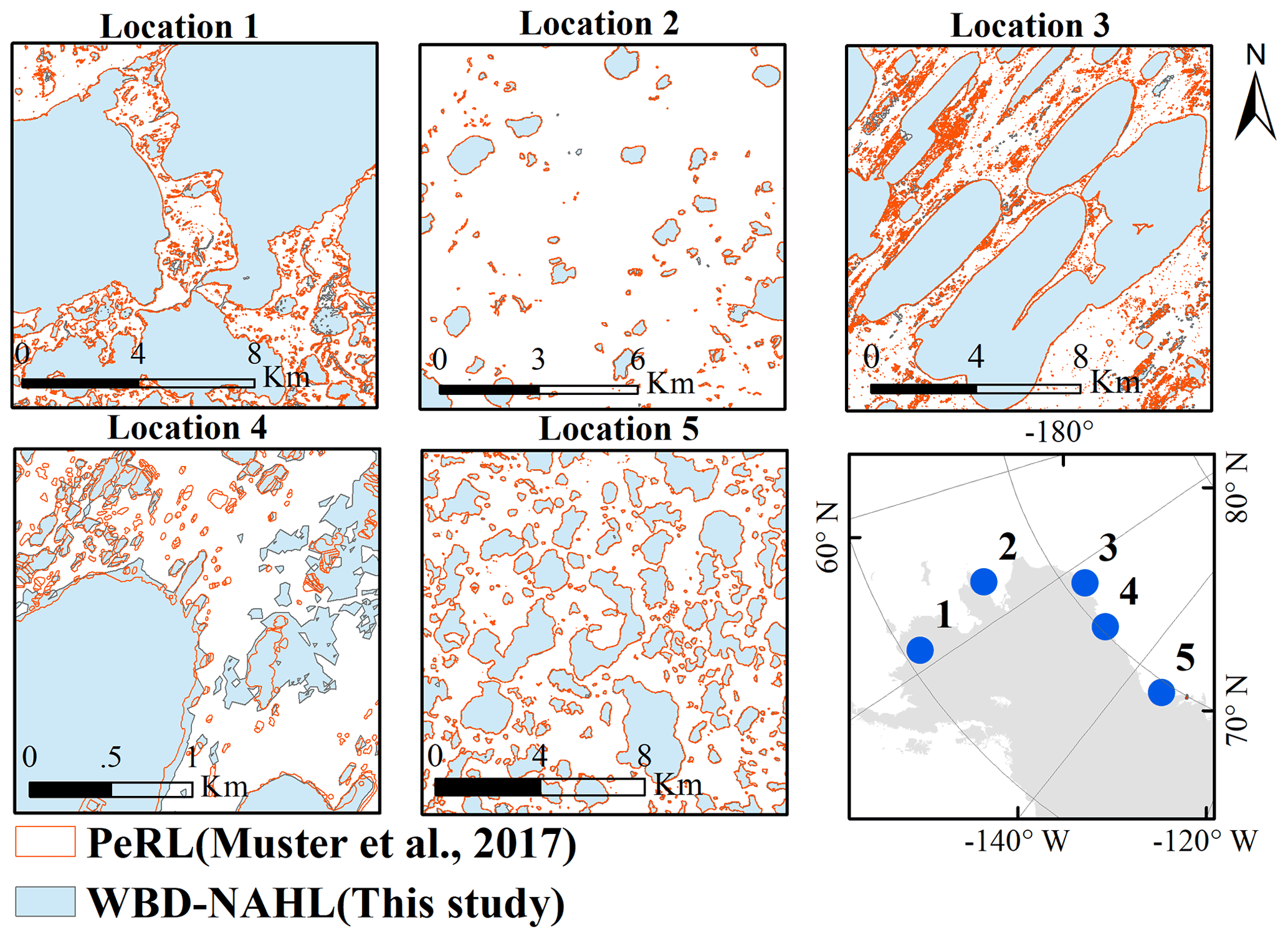
Figure 2 Water bodies identified in the WBD-NAHL (this study) and PeRL datasets (Muster et al., 2017) and the locations (blue dots) of the PeRL maps for the study region.

4 Methods

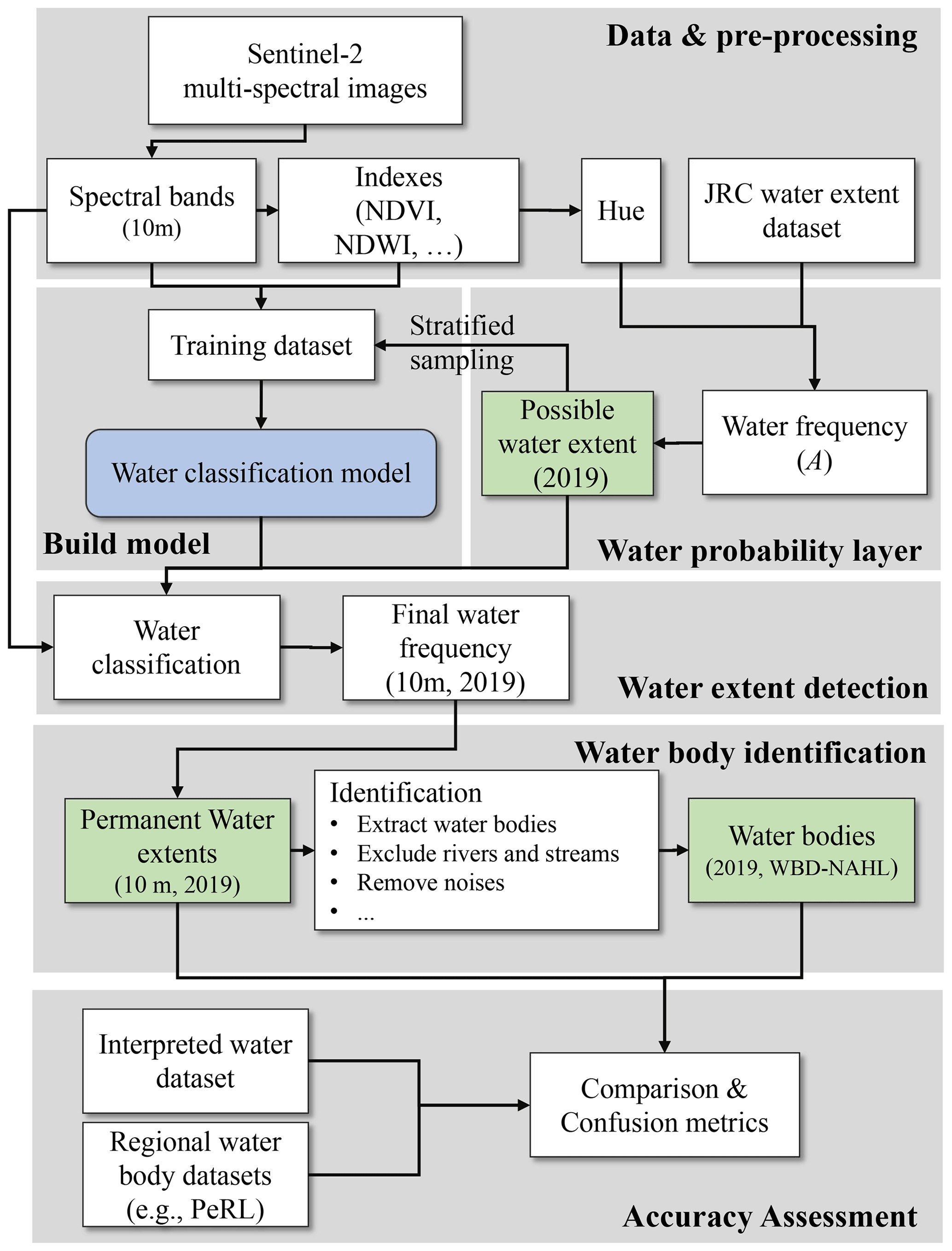
The 10 m resolution Sentinel-2 A and B multispectral data are the primary source used to identify small water bodies. An approach was developed to produce a water probability layer for 2019 by combining the water-sensitive indexes derived from the Sentinel-2 bands and the 30 m resolution JRC water dataset (Sect. 4.1). A machine learning model was trained to retrieve water extent from the Sentinel-2 images from possible water extent restricted by the water probability layer (Sect. 4.2) (Fig. 3). Water bodies were finally identified from the water extent using an object-based algorithm to produce the final water body inventory (Sect. 4.3).

Figure 3 Flowchart for processing water extent and identifying water bodies.

4.1 Water probability layer

A water probability layer was derived to represent the likelihood of a pixel to correspond to permanent water during the summer of 2019. The 10 m resolution water-sensitive indexes calculated from the Sentinel-2 multispectral bands were used as the main input. The other reference water dataset (e.g., the JRC water dataset) was adopted as a supplemental input and fused with the main input to produce the water probability estimate at each 10 m resolution pixel. To reduce effects of snow cover, Sentinel-2 A and B images acquired between June and September 2019 were selected to represent the relatively snow-free season in North American tundra and boreal biomes. The pixels in each Sentinel-2 image with an estimated cloud probability higher than 65 % were excluded to avoid the effects of cloud contamination.

During preprocessing, multiple water-sensitive indexes were derived from each Sentinel-2 image to enhance the ability to detect water (Fig. 3). To maximize the ability to separate water from non-water, especially vegetated land, three indexes were calculated to represent water and vegetation in each image: the Normalized-Difference Water Index (NDWI) (McFeeters, 1996), the Normalized Difference Vegetation Index (NDVI) (Carlson and Ripley, 1997), and the Modified Normalized-Difference Water Index (MNDWI) (Xu, 2006). The three indexes were calculated as follows.

$$\begin{array}{}\text{(1)}& {\displaystyle }\text{NDWI}=(B_{\text{green}}-B_{\text{nir}})/(B_{\text{green}}+B_{\text{nir}}),\text{(2)}& {\displaystyle }\text{NDVI}=(B_{\text{nir}}-B_{\text{red}})/(B_{\text{nir}}+B_{\text{red}}),\text{(3)}& {\displaystyle }\text{MNDWI}=(B_{\text{green}}-B_{\text{swir}})/(B_{\text{green}}+B_{\text{swir}}),\end{array}$$

where B_green, B_red, B_nir, and B_swir are green (band no. 3), red (band no. 4), near-infrared (band no. 8), and short-ware infrared (band no. 11), respectively. These bands have 10 m resolution except B_swir, which has 20 m resolution and was pan-sharpened using the à trous wavelet transform (ATWT) algorithm as recommended by Du et al. (2016). An HSV (hue–saturation–value) color space conversion was used to combine the three indexes and produce a final index for identifying water. The HSV color space conversion is a non-trigonometric pair of transformations from a linear red–green–blue (RGB) color space to a perceived color space (Danielson and Gesch, 2011). This method converts the three input bands into hue (color), saturation, and value components. The three indexes (NDWI, MNDWI, and NDVI) were scaled by 255, converted to a byte value type, combined into the RGB color space, and then converted to the HSV color space to derive a comprehensive index for identifying water.

Once the hue has been identified, an experimental threshold of <0.45 was applied to identify the water pixels. The same procedure was applied to derive temporal water extents from all selected Sentinel-2 images. All the water extents were then combined to calculate the water frequency (A_s) for the year. Potential water extent was then derived from the calculated water frequency data. The existing JRC water dataset provided complementary information for estimating possible water extent. The JRC permanent water records were resampled to 10 m resolution using the nearest-neighbor algorithm and combined with the Sentinel-2-derived water frequency dataset using a weighted linear combination:

$$\begin{array}{}\text{(4)}& A=W_{\mathrm{s}}\cdot A_{\mathrm{s}}+(\mathrm{1}-W_{\mathrm{s}})\cdot A_j,\end{array}$$

where A is the updated water frequency, and W_s is the weight for the Sentinel-2-derived water frequency (A_s), set to 0.85 to ensure that the 10 m measurements were the main input for the final water probability estimate. However, W_s was decreased to 0.65 in high-elevation pixels (elevation>1 km) to reduce the effect of snow and ice on the Sentinel-2-derived hue over mountains. A_j is the JRC permanent water record, which was set to 1.0 for permanent water and to 0.0 for others. The final, combined possible water extent was identified when A>0.5.

4.2 Water extent detection

Although the possible water extent estimated the likelihood of a pixel to correspond to water, confusion with shadow, ice, or cloud contamination in area with complex environments is still possible due to the limitations of water indexes with similar spectra (Isikdogan et al., 2017). A random forest model was trained with points collected through visual interpretations to further detect water within the areas indicated as possible water. To ensure the representation of water and other land covers that can easily be confused as water, five strata were introduced, i.e., water, glacier, mountain, vegetation, and cloud. Then, 250 points were randomly selected in each stratum, for a total of 1250 points (Fig. 4a).

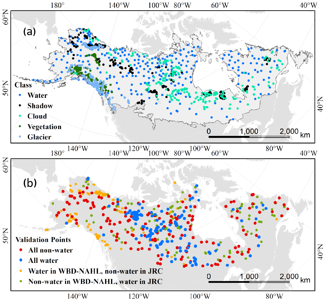
Figure 4 Training samples for random forest model building (a) and points identified for validating the accuracy of the detected water extent (b).

The five strata were established using reference datasets or customized rules. The glacier stratum was identified using the Global Land Ice Measurements from Space (GLIMS) dataset of 2017 (http://www.glims.org/, last access: 7 April 2021), which was a dataset of global glacier outlines including glacier area, geometry, surface velocity, and snow line elevation and was produced from the Advanced Spaceborne Thermal Emission and Reflection Radiometer (ASTER) and the Landsat Enhanced Thematic Mapper Plus (ETM+), as well as historical information derived from maps and aerial photographs. Vegetation was identified as areas with a positive mean NDVI value calculated from the June–September Sentinel-2 images. The cloud stratum was identified as having at least 20 % of mean cloud probability calculated from the selected Sentinel-2 images. The mountain shadow stratum was identified as any elevation higher than 1 km and slope greater than or equal to 3^∘. The water stratum was identified as the remaining area of possible water extent.

The selected points were interpreted by the team to provide training data. Although we only used Sentinel-2 images from June to September 2019, points were matched with a randomly selected image at the location during the time period, providing representation for possible temporal variation. Each point was visually labeled by an interpreter after examining the image. Metrics for visible bands (red, green, and blue), NDWI, MNDWI, NDVI, and hue were derived from each image to provide attributes for the point. These attributes were pooled to produce training data for building the machine learning model.

The scikit-learn Random Forest algorithm (Breiman, 2001) was adopted to build the model for surface water detection. This model was applied to the selected Sentinel-2 images to detect surface water pixels. The results were compiled temporally to produce a water frequency layer (f).

In this study, terrain shadows in the water frequency layer were removed with a terrain mask derived from the Global Multi-resolution Terrain Elevation Data (GMTED) (Danielson and Gesch, 2011). The mask was where the slope was greater than or equal to 7^∘ and the elevation was over 1 km. The elevation threshold was used to minimize the impact of the slope threshold on rivers in lowlands. The method using slope to identify terrain shadows was verified to be more effective than using hillshade (Carroll and Loboda, 2017).

4.3 Water body identification

Permanent water pixels were identified from the resulting water frequency layer (f) as being those pixels with at least 50 % occurrence between June and September. The resulting water pixels were then converted to vector polygons using the “Raster to Polygon” tool in ESRI ArcMap 10.2. These water polygons provided the preliminary surface water body records.

An array of geometry metrics was calculated for each water body polygon using ArcMap in the Canada_Lambert_Conformal_Conic projection (datum D_North_American_1983 and Spheroid GRS80). These metrics include area, perimeter, and a shape index (SI), which estimates the complexity of a water body polygon. The SI was calculated as

$$\begin{array}{}\text{(5)}& \text{SI}=P_{\text{wateri}}/P_{\text{circlei}},\end{array}$$

where P_wateri is the perimeter of the water body I, and P_circlei is the perimeter of a circle that has the same area as water body i. SI equals 1 when a polygon is a perfect circle and greater than 1 when the polygon has a complex irregular shape.

The derived water body morphological metrics (i.e., the SI and area) and the HydroRIVERS were used to identify rivers and streams in the WBD-NAHL water bodies. Rivers and streams tend to have long, narrow, and linear shapes. We applied area thresholds >5 km² and SI>10 in combination with visual examination to exclude large rivers and streams in WBD-NAHL. Considering the extreme difficulties in distinguishing small rivers and streams, water bodies that could possibly be rivers and streams were further identified by selecting long and linear water bodies (SI>3) located close to the rivers and streams (<100 m), as indicated by HydroRIVERS.

4.4 Quality assessment

The accuracy and uncertainty of WBD-NAHL were assessed at two levels, i.e., pixel water extent and derived water bodies, to provide a comprehensive evaluation of the dataset. We randomly selected eight square blocks with a size of 10 km by 10 km in the North American tundra and boreal region (Fig. 5). The selected blocks were visually interpreted by the team to identify all the water bodies within each using a high-resolution Google Earth image as reference for interpretation. Water body records from the PeRL were compared to the WBD-NAHL water bodies to assess the number of water bodies and spatial area of each. The interpreted dataset was also compared to the JRC-derived water body records for 2019 to assess its accuracy in terms of representing water bodies. The JRC dataset provides a water–non-water map at 30 m resolution, representing the distribution of water extent, but no information in the spatial relationship between pixels and water bodies was provided, and we derived water body records from the JRC dataset using the same algorithm described in Sect. 4.1.

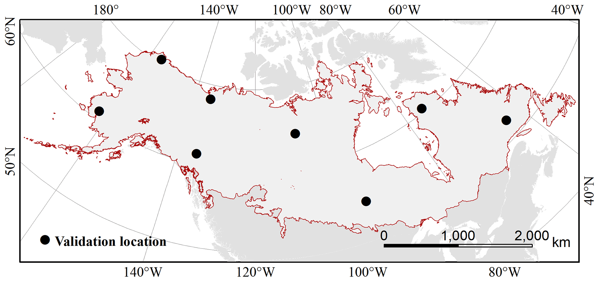
Figure 5 Locations of the five regions selected and interpreted for assessing the accuracy of the indicators of water bodies.

The 14 regional PeRL maps were compared to the WBD-NAHL water bodies. Although the PeRL maps were produced from high-resolution images acquired in 2002–2013, the maps show little temporal change compared to the WBD-NAHL dataset in the extents of the maps (Fig. 2), and these maps were adopted as references for evaluating the WBD-NAHL water bodies. The PeRL maps were produced from images with a resolution of 5 m or finer; we excluded all water bodies in PeRL smaller than 0.0003 km² to ensure comparability to the scale of the WBD-NAHL dataset.

The water extent derived from the Sentinel-2 images was assessed by manually comparing specific points between the WBD-NAHL dataset and the JRC surface water dataset. The points were collected using a stratified random sampling across the entire study region. To achieve higher sampling performance, the outcomes were divided into four strata that represent pixels that were agreed as water, disagreed as water, agreed as non-water, and disagreed as non-water. In each of the strata, 400 points were randomly selected from the dataset and manually assessed by examining the same point in the latest Google Earth image (Fig. 4b). The results from the 1600 points were compared to the derived water extent. The confusion matrix was calculated from the results.

The sampling weights were included in the calculation of the metrics as follows:

$$\begin{array}{}\text{(6)}& W_{\mathrm{s}}=A_{\mathrm{s}}/A_{\text{all}},\end{array}$$

where A_s is the area of stratum s, and A_all is the total area of the region.

The equations of the confusion metrics with weights are

$$\begin{array}{}\text{(7)}& {\displaystyle }\text{OA}=\sum _s^{\mathrm{4}}{W}_{\mathrm{s}}\cdot {\text{OA}}_{\mathrm{s}},\text{(8)}& {\displaystyle }\text{UA}=\sum _s^{\mathrm{4}}{W}_{\mathrm{s}}\cdot {\text{UA}}_{\mathrm{s}},\text{(9)}& {\displaystyle }\text{PA}=\sum _s^{\mathrm{4}}{W}_{\mathrm{s}}\cdot {\text{PA}}_{\mathrm{s}},\end{array}$$

where OA, UA, and PA are the overall accuracy, user's accuracy, and producer's accuracy of the entire dataset; OA_s, UA_s, and PA_s are the concomitant accuracies in stratum s; and W_s is the sampling weight of strata.

5 Results

5.1 Water bodies in tundra and boreal forests of North America

More than 6.47 million (6 474 051) surface water bodies were identified in the tundra and boreal forests of North America, while 90.3 % of these water bodies (5 844 921) were smaller than 0.1 km². Those water bodies covered more than 0.8×10⁶ km², ∼10.3 % of the study area (Fig. 6). The average size and perimeter of the identified water bodies were 0.12 km² and 1.01 km, respectively, and their average SI was 1.41.

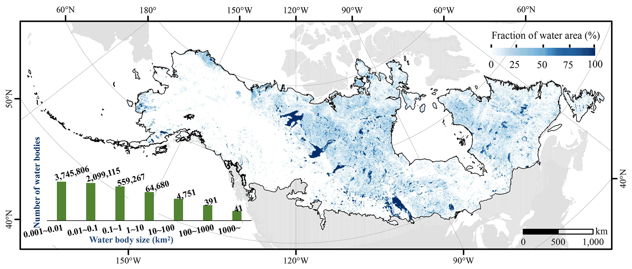
Figure 6 Percent of surface water (5 km×5 km grid) produced by aggregating the water extent for the tundra and boreal forests of North America as calculated using the WBD-NAHL dataset.

All of the morphological indicators, including area, perimeter, and SI, of the identified water bodies showed great heterogeneity across the region (Fig. 7). In general, the tundra biome consists of a large number of densely packed small water bodies with regular shapes. In contrast, the boreal forest biome consists of a large number of large water bodies with complex shapes. The number of identified water bodies in the tundra (3.24 million) and boreal forests (3.23 million) was nearly identical. However, the water extent in the boreal forest (0.57×10⁶ km²; 71 % of total water area) is more than twice that found in the tundra (0.23×10⁶ km²; 29 % of the total water area), indicating that the average size of water bodies in the boreal area is larger than in the tundra. This finding was confirmed by reviewing the water body perimeters for the two biomes. The average perimeter of water bodies in boreal forests was 1.2 km, compared to a much smaller 0.8 km average perimeter for water bodies in the tundra. The average SI for water bodies in the boreal was 1.45, longer than the 1.37 average SI for the tundra water bodies, suggesting that the boreal water bodies generally have much more complex shorelines, while the tundra water bodies are more circular.

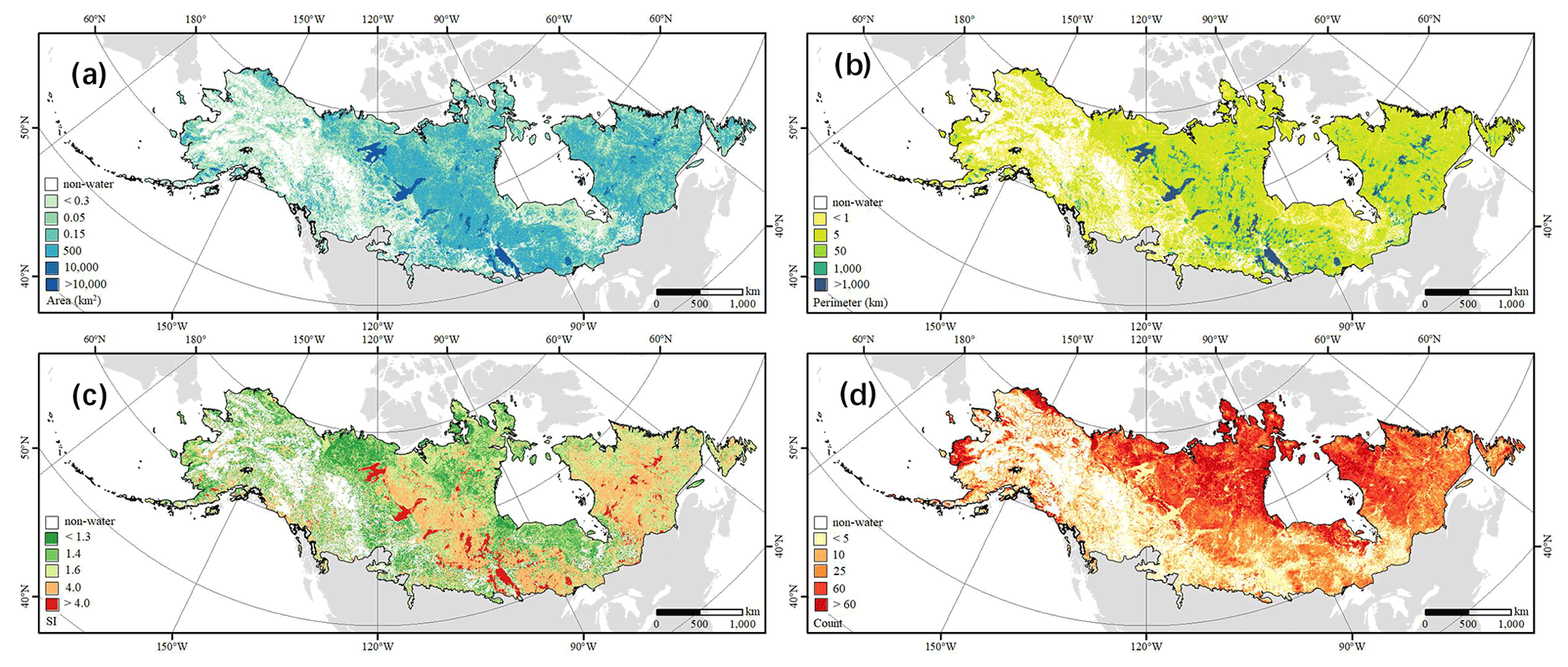
Figure 7 The aggregated distribution of area (a), perimeter (b), and SI (c) and the number (d) of the identified water bodies in the study area. The values at each 5 km×5 km pixel in the grid were calculated by selecting the intersecting water bodies and then either counting or calculating the mean of the targeted parameter (e.g., area, SI, and perimeter) of these selected water bodies.

Inland water in the region is mainly concentrated in the Canadian Shield, i.e., about 0.73×10⁶ km² of water (92 % of water extent in the study region). In addition, most large water bodies were located in the Canadian Shield, including 90 % of the identified large water bodies (sizes≥1 km²). The shorelines of the water bodies in the Canadian Shield were also more complex than those in other areas, especially south of the Laurentian Plateau near the Great Lakes.

5.2 Accuracy assessment

The overall accuracy of the WBD-NAHL's water extent was 96.36 %, while the producer's accuracy was 99.9 %, and the user's accuracy was 96.36 %. Misclassifications were primarily found in shadows of the Mackenzie Mountains, where the east–west high-elevation mountain range cast constant shadows on the northern slopes.

Both the JRC and WBD-NAHL datasets accurately identified the size of larger water bodies. For mixed water pixels, the area estimates of both datasets were more conservative than the reference data. However, the WBD-NAHL dataset performed better than the JRC. The advantage of the WBD-NAHL was demonstrated for smaller water bodies (Fig. 8). For small water bodies (size≤0.02 km²), the average area of the WBD-NAHL water bodies was 72 % of those manually digitized over high-resolution Google Earth images, compared to only 45 % with the water area detected by the JRC (Fig. 8a). For medium water bodies (between 0.02 and 0.05 km²), the average area of WBD-NAHL water bodies was about 85 % times that of manually digitized water bodies, compared to 67 % with the water area detected by the JRC (Fig. 8b). For water bodies larger than 0.05 km², the water areas of WBD-NAHL were highly consistent (98 %) with that of manually digitized, while the water area of JRC was slightly lower (about 87 %) for water bodies in the category (Fig. 8c).

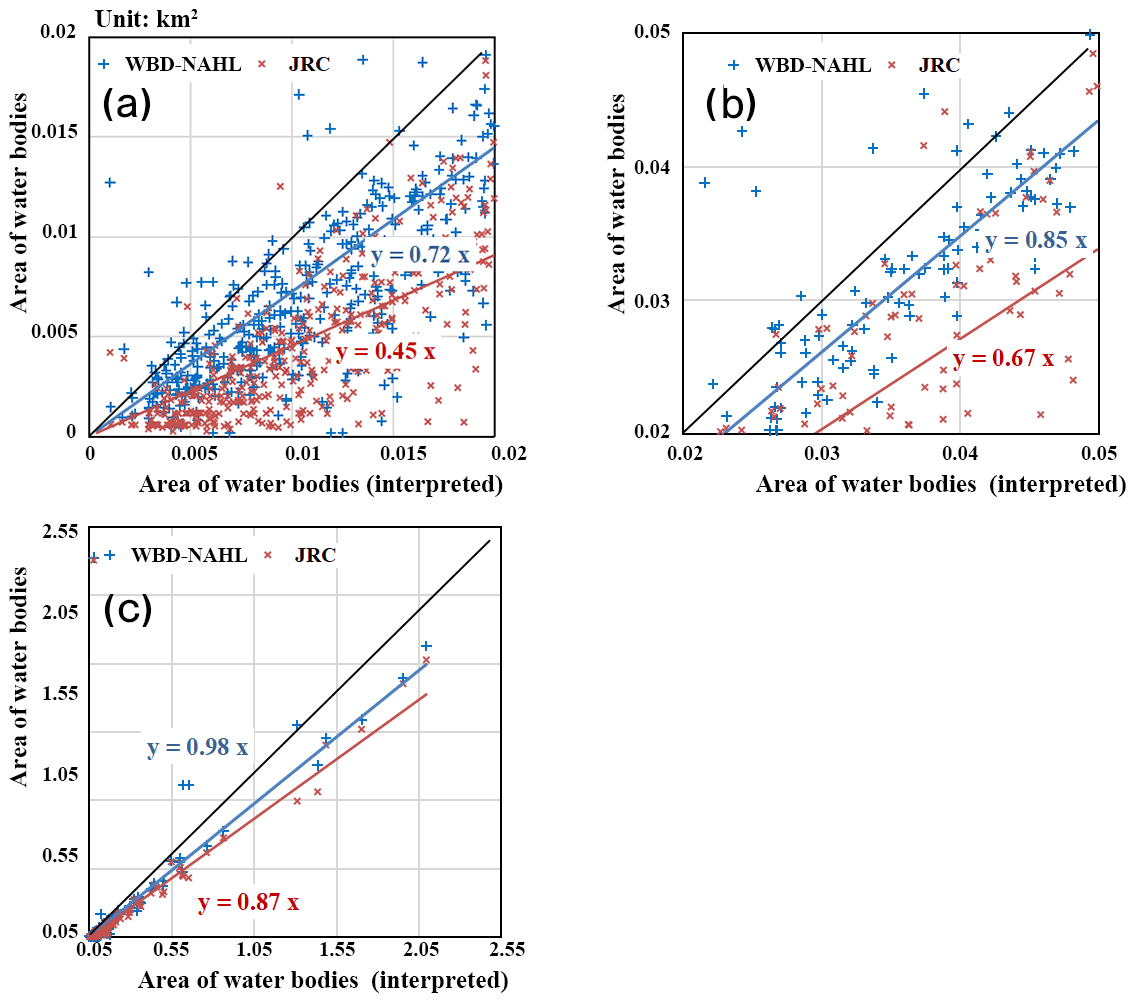
Figure 8 Comparisons of the water body area identified by the JRC, WBD-NAHL, and interpreted water maps. The 1:1 lines are in black. The red crosses represent the JRC water bodies, and the blue pluses represent the WBD-NAHL water bodies in comparison with the manually interpreted water bodies. The water bodies are compared in groups of sizes, i.e., (a) small water bodies with sizes <0.02 km², (b) medium water bodies with sizes between 0.02 and 0.05 km², and (c) large water bodies with sizes >0.05 km². The R² values for the WBD-NAHL and JRC identified water bodies were similar, i.e., 0.6 for small water bodies, 0.5 for medium water bodies, and 0.9 for large water bodies.

The comparison between the water bodies identified by WBD-NAHL and PeRL was largely consistent for the derived indicators of water area, perimeter, and number (Fig. 9). Linear correlations between the water bodies identified by WBD-NAHL and PeRL had R² higher than 0.99 for all three indicators. The slopes of the linear regressions indicated that the water area showed the least bias when compared to PeRL (slope=0.98), followed by the number of water bodies (slope=0.78), and finally the perimeter of the water bodies (slope=0.62).

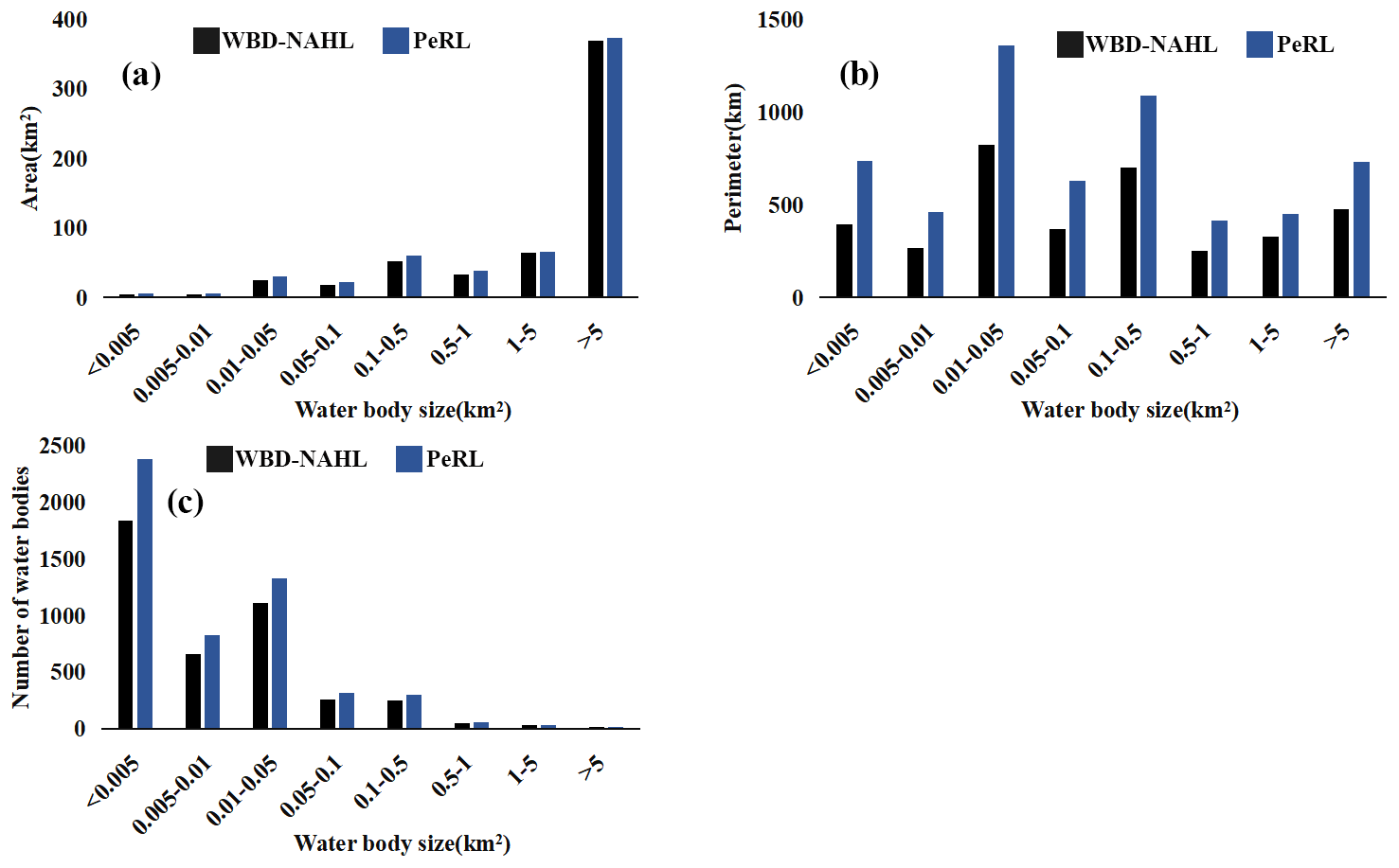
Figure 9 Area, perimeter, and number of water bodies identified by the PeRL and WBD-NAHL datasets.

6 Discussion

6.1 A high-resolution water body dataset for the continental tundra and boreal

The WBD-NAHL dataset provides the first known delineation of water bodies at 10 m resolution for the continental tundra and boreal forest of North America, which is one of the highest concentrations of the global inland water, especially the small-sized water bodies. The dataset not only maps the extent of inland water during 2019, but also identifies the water bodies and their morphological metrics, which are critical for understanding and modeling freshwater lentic ecosystems (Downing, 2009; Heathcote et al., 2015; Kuhn and Butman, 2021; MacIntyre et al., 2009; Muster et al., 2013). The WBD-NAHL dataset was produced using Sentinel-2 satellite data to take advantage of the high resolution and 2–3 d revisit time of Sentinel-2 satellites. Sentinel-2's revisit time allows the WBD-NAHL to have sufficient observations during the snow-free season, which is critical for mapping inland surface water in this high-latitude region with long periods of snow coverage.

The WBD-NAHL's 10 m resolution enabled detection of water bodies as small as 0.001 km². The validation showed that the WBD-NAHL dataset had high overall accuracy and significantly improved upon the ability of the existing global JRC water maps for detecting small water (e.g., smaller than 0.006 km²) than the existing global JRC water maps. These small water bodies consist of nearly half the total water bodies in the tundra and boreal forest regions of North America and generally experience faster cycling of water, material, and energy than larger water bodies (Winslow et al., 2014; Carroll et al., 2011; Messager et al., 2016). The improved WBD-NAHL dataset may provide more accurate inputs for hydrological estimates, which are vital components for understanding and modeling the pan-Arctic hydrological, biochemical, and energy cycling.

The higher resolution of WBD-NAHL also provides the ability to delineate the number, area, and shoreline complexity of water bodies. Our comparison confirmed that WBD-NAHL-derived water areas and shorelines were similar to those from the regional PeRL dataset with a resolution of 5 m or finer. Meanwhile, the number of water bodies identified in WBD-NAHL was consistent with that of other datasets, including HydroLAKES and GLWD (Fig. 10). The number of water bodies larger than 1 km² was roughly identical for WBD-NAHL, HydroLAKES, and GLWD. For water bodies between 0.1 and 1 km², WBD-NAHL and HydroLAKES reported similar numbers (Fig. 10), but the number reported by GLWD was considerably lower, suggesting that the omission error of GLWD was higher for water bodies smaller than 1 km², as noted by Lehner and Döll (2004). Unfortunately, both the HydroLAKES and GLWD datasets only provide records for water bodies larger than 0.1 km² (Messager et al., 2016; Lehner and Döll, 2004) and are thus missing records for what we estimate to be 90 % of the total number of water bodies in the region. The WBD-NAHL dataset is able to extend these indicators to much smaller water bodies than HydroLAKES and GLWD, providing a much more complete record of water bodies in the region. This estimate of the number and extent of small water bodies can improve our understanding of continental freshwater sources, stressing the importance of small water bodies in continental biochemical and energy cycling, potentially correcting a misconception that large lakes are most important (Downing, 2010).

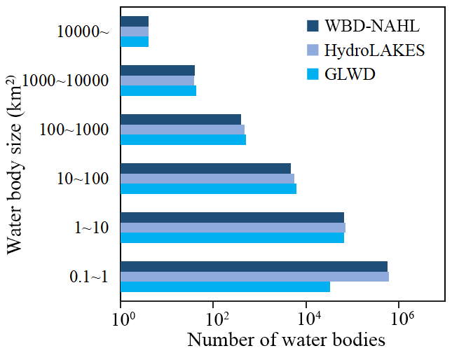
Figure 10 Comparing the number of water bodies identified by WBD-NAHL and other datasets based on size.

6.2 Distribution of the water bodies

An empirical power-law distribution was found between lake areas and lake numbers (Messager et al., 2016; Downing et al., 2006), and the distribution was applied to estimate the number of small lakes, which were used for estimating greenhouse gas emissions (Holgerson and RAymond, 2016). According to the power-law distribution and HydroLAKES, the number of water bodies larger than 0.1 km² was estimated to be about 798 895, which was close to the 629 130 water bodies reported by WBD-NAHL (Fig. 11). However, the number of water bodies sized between 0.1 and 0.01 km² was estimated to be about 10.2 million, 4.8 times higher than estimated by WBD-NAHL. Furthermore, the water bodies sized between 0.01–0.001 km² were estimated to be about 126.1 million, 33.6 times higher than what was estimated by WBD-NAHL, suggesting that the power-law distribution significantly overestimates the number of small lakes. A similar finding was reported by Cael and Seekell (2016). Estimating the number small water bodies using a power-law distribution could introduce considerable uncertainties in the estimation of the contribution of small water bodies to greenhouse gas emissions. Accurately identifying small water bodies could correct this overestimation and improve greenhouse gas emission estimates (Holgerson and Raymond, 2016).

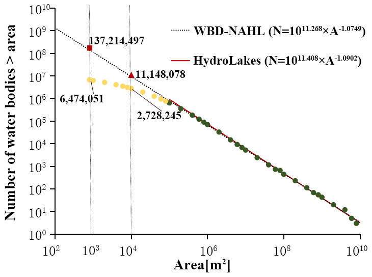
Figure 11 Distribution of the total numbers of water bodies in relation to the area of North American tundra and boreal forests water bodies. The circles represent the number of water bodies provided by WBD-NAHL. The black line is the power-law distribution modeled using water bodies >0.1 km² from WBD-NAHL. The red line is the power-law distribution modeled using HydroLAKES in the study region. The red triangle and square represent, respectively, the extrapolated number of water bodies >0.01 and >0.001 km² based on the power-law distribution modeled from HydroLAKES.

The largest and most complex water bodies are distributed primarily in the Canadian Shield. These lakes in the Canadian Shield formed through processes such as erosion and glaciation (Smith et al., 2007). Erosion and glaciation formed water bodies with complex shapes, which may contribute to the higher SI (1.48) reported by the WBD-NAHL for the region. During the most recent Wisconsin glaciation, the Canadian Shield was covered by the Laurentide Ice Sheet, a giant, 3 km thick expanse of ice. When the ice sheet retreated north, it carved out the five Great Lakes as well as thousands of small lakes throughout the Canadian Shield (Dyke and Prest, 1987). Currently, 92 % of the water extent in the tundra and boreal forests are distributed in this particular region. For example, the largest lake in the region – Great Bear Lake – has a surface area of 30 227 km² with a long, complex shoreline (the perimeter is 5705 km, and the SI of the lake is 9.3). It was formed by ice erosion during the Pleistocene (Johnson, 1975).

The tundra, on the other hand, has a large number of small, regularly shaped water bodies, which could be related to the thick peatland and thermokarst landscape. Over the past few decades, numerous thermokarst lakes have been experiencing dramatic changes, which are considered an indicator of permafrost degradation (Smith et al., 2005; Karlsson et al., 2012, 2014). The small thermokarst lakes were also found to experience stronger changes than larger lakes (Karlsson et al., 2014; Carroll and Loboda, 2017). Monitoring water extent without discriminating by lake size does not accurately reflect these changes in small lakes due to the area dominance of large lakes. Additionally, the small thermokarst lakes are the primary source of permafrost carbon emissions (Kuhn et al., 2018; Walter Anthony et al., 2016; Yvon-Durocher et al., 2017), and small water bodies were found to be a major source of uncertainty greenhouse gas emission estimates (Holgerson and Raymond, 2016). The WBD-NAHL dataset could provide critical information for investigating thermokarst lakes, especially small thermokarst lakes and ponds, and estimate their effects on carbon emission and permafrost sustainability in the tundra and boreal forests of North America. As reported by the analysis of WBD-NAHL, 3.24 million small water bodies were found in the tundra in 2019, with an average size of 0.07 km² and average SI of 1.37, much smaller than the SI of boreal lakes. Teshekpuk Lake is the largest thermokarst lake in the world and has a relatively smooth shoreline (SI=5.4), considerably smaller than the SI of Great Bear Lake in the boreal region (Markon and Derksen, 1994).

The biome-based analysis provided insights into the distribution of water body shapes across the study area; however, more complex relationships can be found between the shapes and the surface geology of the water bodies. For example, circular-shaped lakes can be found in regions with thick overburden – possibly as a result of being unglaciated, from aeolian deposits or from rising from the sea bottom through isostatic rebound. These circular-shaped lakes can be found in regions with thick moraines or widespread peatlands in the boreal Hudson Bay lowlands and the Mackenzie River Basin. The high-resolution WBD-NAHL could help further explore the distribution of water bodies by size and shape.

6.3 Limitations

The data and methods used to derive the 10 m resolution WBD-NAHL dataset are able to detect water bodies smaller than the 30 m resolution or coarser-resolution satellite-derived datasets but have difficulty identifying water bodies smaller than 0.001 km². This limitation can be further improved by incorporating higher-resolution satellite data, such as from Planet, WorldView, QuickBird, and Gaofen (Sun et al., 2020; Watson et al., 2016; Andresen and Lougheed, 2015). Limit errors in the satellite data provide substantial sources of uncertainty, including an inability to separate rivers and streams because the resolution is too coarse, bias in estimates of water extent resulting from temporal gaps in the data, and misclassifications resulting from spectral resolution. The misclassifications impacted by terrain (e.g., mountain shadows) still exist, even though they have been substantially reduced during data processing. Further processing may be possible to further reduce these errors.

The WBD-NAHL dataset was produced based on Sentinel-2 data acquired in the summer of 2019 and represents the distribution of surface water in the corresponding year. The mean total precipitation in 2019 in the region was 438.5 mm, which was close to the historical average from 2010 to 2019 (mean: 435.9 mm, standard deviation: 11.5 mm) (Huffman et al., 2019). Although 2019 can be considered a normal year of the past decade in terms of precipitation, the spatial extent of high-latitude water bodies, especially smaller water bodies, can still vary significantly both inter- and intra-annually locally. Nevertheless, it would be interesting to explore water bodies' changes using observations from multiple years. Further efforts can be carried out to produce an inland water dataset for multiple time periods using these methods to capture the seasonal and multi-year dynamics of inland water in the region. The WBD-NAHL dataset focused on the tundra and boreal forest regions of North America. The methodology can be extended to Eurasia to provide a complete representation of the biomes.

7 Data availability

This WBD-NAHL dataset can be accessed via the website of the National Tibetan Plateau/Third Pole Environment Data Center (TPDC; http://data.tpdc.ac.cn, 6 June 2022): https://doi.org/10.11888/Hydro.tpdc.271021 (Feng et al., 2020). The dataset is provided in ESRI Geodatabase format. The volume of this dataset is about 1.5 GB.

8 Conclusions

This study presents an inland surface water body dataset for the North American high latitudes. The WBD-NAHL dataset was generated using Sentinel-2 data with machine learning methods and an object-based algorithm. Three morphological metrics (area, perimeter, and SI) were calculated for each water body. The accuracy of the dataset was carefully assessed with respect to detecting inland surface water extent (or pixel level) and identifying water bodies. The dataset's overall accuracy for water extent reached 96.36 %. In addition, the WBD-NAHL showed a high consistency with high-resolution images in terms of water area, perimeter, and quantity.

To our knowledge, the WBD-NAHL dataset provided the most complete inventory of inland surface water bodies for the tundra and boreal forest regions of North America. Overall, 6.47 million water bodies were identified, covering 10.3 % of the region. Small water bodies dominate the region, as ∼90.3 % have an area smaller than 0.1 km². The WBD-NAHL dataset indicates that the tundra biome is dominated by densely distributed small water bodies with regular shapes (the average SI was 1.37), while the boreal forest biome is dominated by large water bodies with complex shapes (the average SI was 1.45). The WBD-NAHL dataset is expected to be able to provide supporting data for modeling hydrologic, biochemical, and energy cycling in these areas.