the Creative Commons Attribution 4.0 License.
the Creative Commons Attribution 4.0 License.
 | 10 Jan 2022
EUREC4A's Maria S. Merian ship-based cloud and micro rain radar observations of clouds and precipitation
Claudia Acquistapace
Richard Coulter
Susanne Crewell
Albert Garcia-Benadi
Rosa Gierens
Giacomo Labbri
Alexander Myagkov
Nils Risse
Jan H. Schween
As part of the EUREC4A field campaign, the research vessel Maria S. Merian probed an oceanic region between 6 to 13.8∘ N and 51 to 60∘ W for approximately 32 d. Trade wind cumulus clouds were sampled in the trade wind alley region east of Barbados as well as in the transition region between the trades and the intertropical convergence zone, where the ship crossed some mesoscale oceanic eddies. We collected continuous observations of cloud and precipitation profiles at unprecedented vertical resolution (7–10 m in the first 3000 m) and high temporal resolution (1–3 s) using a W-band radar and micro rain radar (MRR), installed on an active stabilization platform to reduce the impact of ship motions on the observations. The paper describes the ship motion correction algorithm applied to the Doppler observations to extract corrected hydrometeor vertical velocities and the algorithm created to filter interference patterns in the MRR observations. Radar reflectivity, mean Doppler velocity, spectral width and skewness for W-band and reflectivity, mean Doppler velocity, and rain rate for MRR are shown for a case study to demonstrate the potential of the high resolution adopted. As non-standard analysis, we also retrieved and provided liquid water path (LWP) from the 89 GHz passive channel available on the W-band radar system. All datasets and hourly and daily quicklooks are publically available, and DOIs can be found in the data availability section of this publication. Data can be accessed and basic variables can be plotted online via the intake catalog of the online book “How to EUREC4A”.
- Article
(10682 KB) - Full-text XML
- BibTeX
- EndNote


Clouds and precipitation in the tropics are crucial for radiative budget and are responsible for climate prediction uncertainties (Bony and Dufresne, 2005). From 19 January to 19 February 2020, the “EUREC4A: A Field Campaign to Elucidate the Couplings Between Clouds, Convection and Circulation” campaign (Bony et al., 2017) took place in the Atlantic waters southeast of Barbados to test hypotheses on trade wind cumuli cloud feedbacks. Stevens et al. (2021) describe how the campaign's initial scope greatly expanded towards additional research questions, extending the campaign area and the number of scientific platforms involved. To understand the factors influencing rain formation, study the evolution of mesoscale oceanic eddies and their impact on air–sea interactions, and produce a dataset that can stand as a benchmark for future model evaluations and satellite retrievals became complementary goals of the enlarged campaign. Within EUREC4A, the Ocean-Atmosphere component (EUREC4A-OA, https://eurec4a.eu/overview/eurec4a-oa/, last access: 18 December 2021) was granted two research vessels (R/Vs) in the Atlantic sea southeast of Barbados to monitor the oceanic processes induced by large-scale oceanic eddies.
The R/V Maria Sybilla Merian (MS Merian) was deployed in the southern part of the EUREC4A domain to investigate how mesoscale oceanic eddies impact oceanic circulation and their role in cloud and precipitation formation. The collaboration with the ARM Mobile Facility 2 (https://www.arm.gov/capabilities/observatories/amf, last access: 20 December 2021) equipped the R/V with a comprehensive suite of remote sensing instrumentation that could track each stage of the precipitation life cycle. A micro rain radar (MRR) and a cloud radar (W-band) were installed on a stabilization platform: while the W-band radar is sensitive to a wide range of atmospheric scatterers from tiny cloud drops to raindrops, the MRR can adequately describe the sub-cloud layer's rain evolution. The 89 GHz passive channel available in the W-band radar system allowed us to characterize the columnar amount of liquid water, and integrated water vapor was retrieved only in clear-sky conditions by means of a linear regression with co-located radiosoundings. All W-band and MRR radar variables are listed in Sect. 2.1 and 2.2.
The collaboration with ARM and the use of their stabilization unit allowed the compensation for ship motion and for the first time made it possible to obtain essential Doppler observations at unprecedented spatial and temporal resolution of the entire precipitation life cycle.
This radar suite represents one of the most advanced remote sensing setups for measuring trade wind precipitation in and below the cloud. Ground-based cloud radar remote sensing has been used for a long time to monitor the vertical structure of clouds and precipitation (Bretherton et al., 2010; Lamer et al., 2015; Leon et al., 2008; Kollias et al., 2007), as well as on ships (Zhou et al., 2015). In recent years, the potential of new observables like the Doppler spectra's skewness to detect precipitation forming in the cloud (Kollias et al., 2011b, a; Luke and Kollias, 2013; Acquistapace, 2017) was demonstrated for fixed ground-based sites. However, shipborne cloud radar Doppler measurements have not been exploited yet. A first analysis of the unique dataset of trade wind cumulus clouds and precipitation collected with the MRR and the W-band radar on MS Merian is presented. Considering typical sea wave periods of 9 s, to obtain Doppler observations at sea, integration times have to be chosen shorter than 1 s (Chris Fairall, personal communication, 2020). In the paper, we document how specific choices on the integration times of the instruments were made, describing the measurement sampling strategy regarding spatial and temporal resolution.
The synergistic usage of the dataset collected on the R/V will be crucial for tackling precipitation life cycle detection using a multiscale approach based on the additional measurements on board not presented here: a water vapor Raman lidar and a wind lidar from the University of Hohenheim; a cloud kite from the Max Planck Institute for Dynamics and Self-Organization of Göttingen (http://www.lfpn.ds.mpg.de/MCO/ck.html, last access: 18 December 2021), that is a 250 m3 balloon able to fly up to 2500 m for in situ observations of cloud and raindrop size distributions; 3D wind profiles; and eddy dissipation rates. When combining the W-band radar and the co-located in situ observations from the cloud kite, a detailed description of the precipitation process and unique reference data for high-resolution model runs become available. The high vertical (7–10 m) and temporal (1–3 s) resolution adopted by all the active remote sensing instrumentation below 2500 m will constitute an essential benchmark for future satellite missions like EarthCARE (Illingworth et al., 2015), providing a detailed description of the atmospheric layer closer to the surface that is and will be the most critical region to detect from satellites (Lamer et al., 2020). The 1-month precipitation data collected during the campaign also represent a vital evaluation dataset for Global Precipitation Measurement (GPM) mission performance at sea in the subtropics for shallow convection precipitation (Hou et al., 2014). The stabilization platform worked for approximately 65 % of the time, while for 35 % of the time it did not, and we considered ship motion corrections for both situations. Similar methods have been derived for airplane-based measurements with Doppler measurements (see, e.g., Bange et al., 2013). The track followed by the R/V MS Merian allows us to characterize the latitudinal dependency on the cloud fields when moving from the subtropics towards the inter-tropical convergence zone and understand the impact of the sea surface temperature heterogeneities on the boundary layer (Laxenaire et al., 2018). We collected some lessons learned during the EUREC4A campaign with the hope of encouraging and facilitating future deployments of active remote sensing instruments on ships, given the strategic importance that such data might have.
The paper is organized as follows. Section 2 describes the experimental setup and the instrument characteristics. Section 3 provides details on the data processing and on the removal of the interference pattern from the data, assessing the impact of the ship motion correction algorithm. Section 4 describes a case study of trade wind cumulus clouds and precipitation. We describe how to access data and processing scripts in Sect. 5, while Sect. 6 briefly collects the lessons learned and Sect. 7 summarizes the work.

Figure 1Instrument deployment on the R/V MS Merian. (a) View of the top deck (so-called Peildeck): the hydraulic unit is visible on the right in the metal box, connected via multiple cables to the stabilization platform. (b) The MRR (left) and the W-band radar (right) fixed using two metal bars on the stabilization platform. (c) Position of the instrument deployment with respect to the motion reference unit (MRU) on the MS Merian: side view (left) and front view (right).
We positioned the radar equipment on the R/V's top deck at around 20 m above sea level, as far as possible from the influence of sea spray (Fig. 1). The W-band radar and the MRR were mounted on the stabilization platform using two metal bars. To limit vibrations, we installed rigid support between the MRR's pole and the W-band radar. At installation, we synchronized the internal clocks of the computers controlling the radar equipment with the ship navigation system clock. Despite this effort, the time stamp synchronization suffered from a drift of the clocks with respect to the Global Positioning System (GPS) time of the ship's inertial system variable between 1 and 4 s that we had to consider in the correction of the data for ship motions. From 19 January to 19 February 2020, the R/V MS Merian sailed over a vast oceanic region spanning from 6 to 13.8∘ N and from 51 to 60∘ W (see Fig. 2). We launched 118 radiosondes and collected 38 descents to provide temperature (T), pressure (P), and humidity (q) profiles during the whole campaign (Stephan et al., 2021). This database was used to build a retrieval for integrated water vapor from the single passive 89 GHz channel available on the W-band radar. In the following, we will first describe the two radars followed by the stabilization platform, and we will describe the motion reference unit (MRU) and the ship reference system.
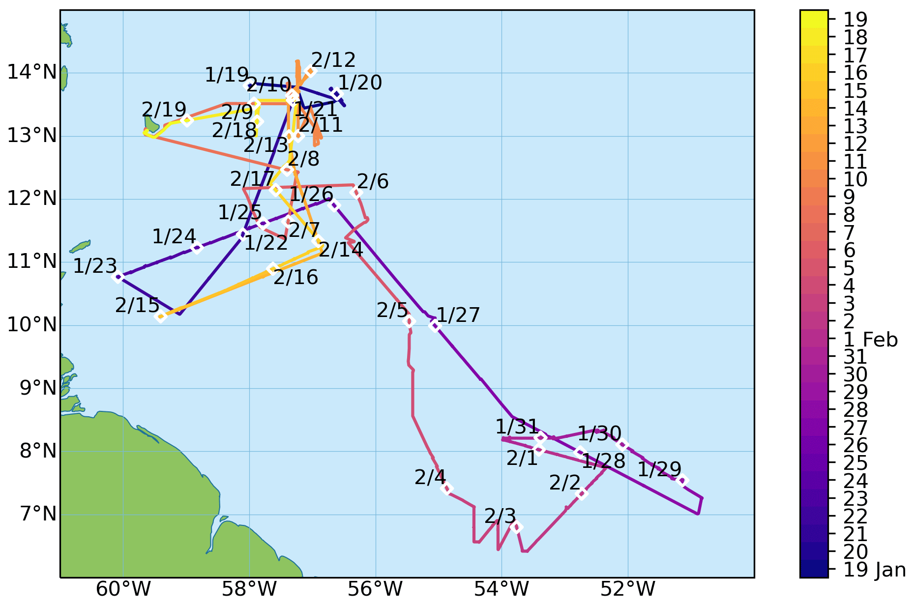
Figure 2Ship track of the R/V MS Merian during the EUREC4A campaign, from 19 January to 19 February 2020.
2.1 W-band radar
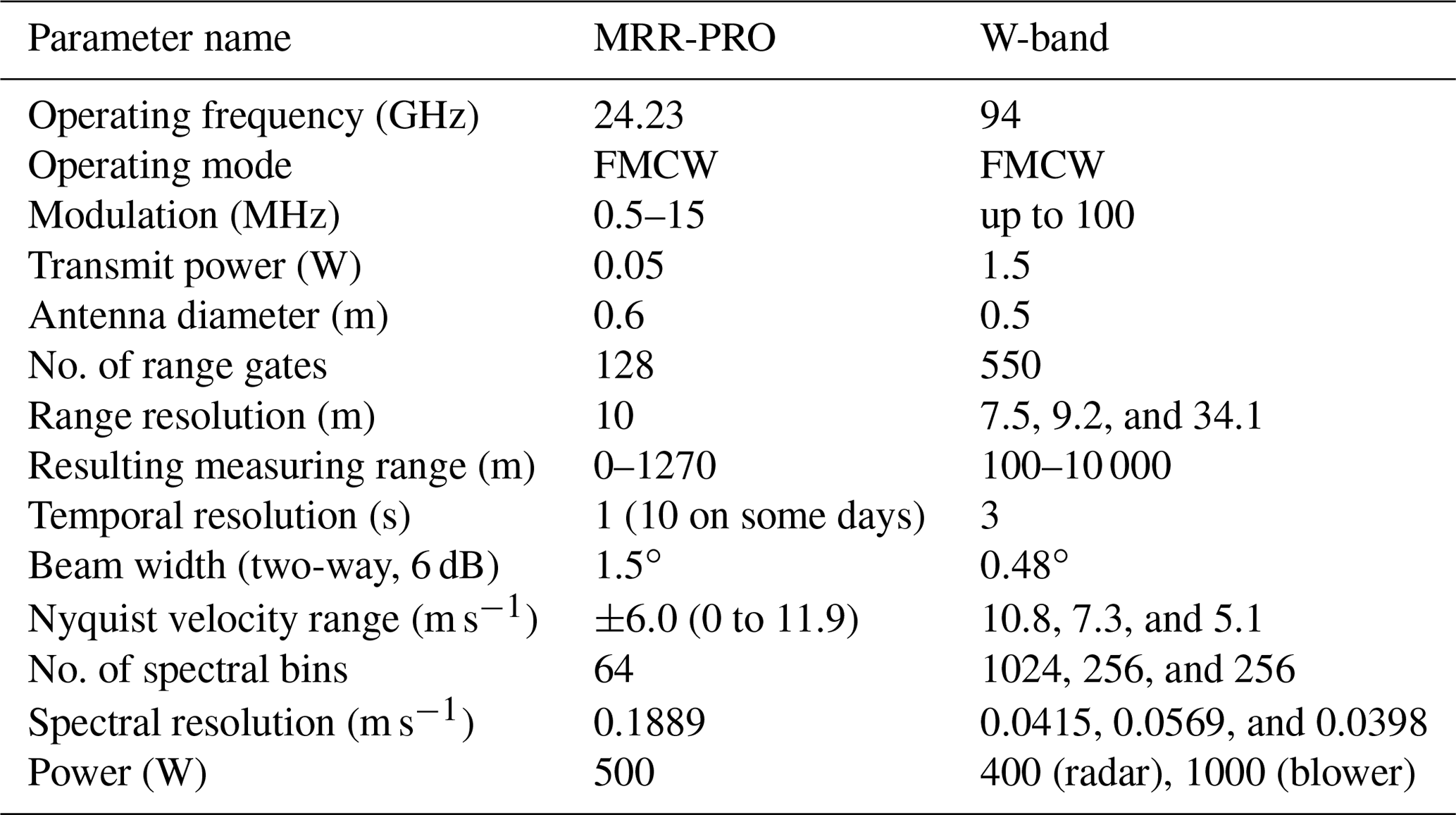
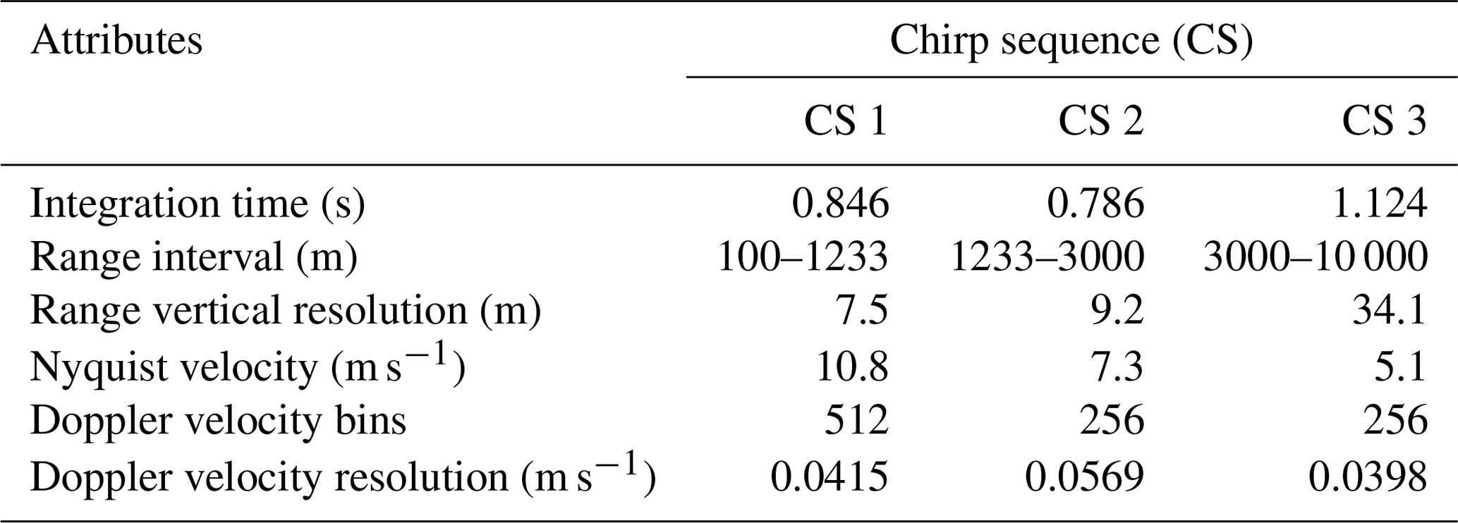
The W-band radar is a frequency-modulated continuous-wave (FMCW) 94 GHz dual-polarization radar equipped with a radiometric channel at 89 GHz and is manufactured by Radiometer Physics GmbH (RPG), Germany. The small diameter of its antennas (0.5 m), one to transmit and one to receive, and its compactness (Table 1) make it a well-suited instrument to be deployed in complex environments. Küchler et al. (2017) provided an extended description of the radar performance, hardware, calibration, and signal-processing procedures. We calibrated the receiver of the W-band radar after installing it in the position shown in Fig. 1. To protect the hydrophobic radome from hydrometeors, the radar is equipped with a blower for both antennas. The blower is able to produce a thin airflow with up to 20 m s−1 over the antenna radomes (Küchler et al., 2017). Users can set different range resolutions at different altitudes by providing the necessary parameters to the so-called “chirp table”, i.e., a table storing all the frequency modulation settings. Table 2 shows the chirp table definition adopted for this measurement campaign. We defined the chirp table to have a high vertical resolution below the inversion layer to focus on shallow cumulus clouds (Table 2). This choice resulted in reaching a maximum detectable range of 10 000 m to focus on high vertical resolution of the boundary layer clouds and the inability to measure high cirrus clouds. The range resolution from the sea level to 1233 m was 7.5 m, while it was 9.2 m between 1233 and 3000 m. Between 3000 and 10 000 m the range resolution was 34.1 m. We chose integration times of 0.846 s for heights smaller than 1233 m, 0.786 s between 1233 and 3000 m, and 1.124 s between 3000 and 10 000 m to make the ship motion correction effective. The total sampling time required to measure a full profile resulted in around 3 s.
The embedded passive channel operates at 89 GHz with a bandwidth of 2 GHz and measures the calibrated brightness temperature (TB). In the W-band, atmospheric gases are relatively transparent. The absorption coefficient of atmospheric gases in the lower troposphere is of the order of 1 dB km−1 (Ulaby et al., 1981). In contrast, cloud liquid water produces a strong attenuation (≈1 dB km−1 g−1 m3; Ulaby et al., 1981) in this frequency band. Since the passive measurements are sensitive to the presence of liquid water, the TB measured at 89 GHz can be used in a retrieval of liquid water path (LWP) (Küchler et al., 2017). The cloud radar continuously runs a statistical retrieval developed by the radar manufacturer. The retrieval is based on an artificial neural network (ANN), which approximates values of LWP for a given set of the observed TBs, surface temperature, relative humidity, pressure, and day of the year. For the ANN training, a dataset of atmospheric profiles was used. Since the ship was moving around Barbados during the campaign, data from several surrounding stations were combined in the dataset. The dataset consisted of three radiosonde stations and one ERA-Interim reanalysis column (Dee et al., 2011). For more details on the ANN and the dataset used for it, please refer to Appendix A and Table A1.
We obtained integrated water vapor (IWV) estimates by applying a single-channel retrieval in clear-sky cases, defined as profiles where all W-band radar reflectivity values are smaller than −50 dBz. The retrieval is based on the quadratic regression between the 89 GHz brightness temperatures and the IWV estimated with the radiosoundings. We selected all radiosoundings with relative humidity smaller than 97 % in the entire profile launched when no cloud base was detected by the wind lidar on board MS Merian. The IWV results from integrating the profile of specific humidity over height and is associated with the mean 89 GHz brightness temperature calculated over 1 min after the radiosonde launch.
The W-band radar data collected during the EUREC4A campaign have been post-processed using a software package that includes processing and de-aliasing of compressed and polarized spectra. The code is an update and a subsequent restructuring of the first program version provided by Küchler et al. (2017), and it is available at https://github.com/igmk/w-radar/tree/new_output_structure (last access: 23 December 2021). No liquid attenuation correction has been applied to the data yet. The post-processing routine produces as output a technical data file including all radar specific variables and a physical data file, available in two versions. One version (compact), structured as daily files, includes
-
radar moments (equivalent reflectivity factor (from now on called reflectivity), mean Doppler velocity negative towards the ground, Doppler spectral width, Doppler spectrum skewness, Doppler spectrum kurtosis);
-
coordinates (time, height, latitude, longitude);
-
integrated variables (liquid water path, brightness temperature at 89 GHz);
-
surface variables collected by the meteo station attached to the radar (wind speed and direction, pressure, temperature, rainfall rate, and humidity);
-
general parameters (file code/version number, compression flag).
The other version (complete radar data), organized in hourly files, includes all the previous variables plus additional radar variables like the Doppler spectrum, the bin mean noise power, and the sensitivity limit. In addition to the standard processing, we derived and added the mean Doppler velocity field corrected for ship motions to the variables listed above in both versions of the files. The compact version has been enhanced with Climate and Forecast (CF) conventions (https://cfconventions.org/, last access: 23 December 2021) to allow online plotting using the EUREC4A book (https://howto.eurec4a.eu/intro.html, last access: 23 December 2021). Section 3.1 and 3.2 describes the post-processing applied to the data, and Sect. 5 explains the available data products.
2.2 Micro rain radar
The micro rain radar (MRR) deployed on the R/V MS Merian is a vertically pointing frequency-modulated continuous-wave (FMCW) Doppler radar operating at 24.23 GHz, produced by the Meteorologische Messtechnik GmbH (Metek) (Peters et al., 2002) and owned by the University of Leipzig. The instrument deployed was the latest version of the MRR, the so-called MRR-PRO, with an antenna diameter of 0.6 m (Fig. 1), and comes with a factory calibration. Table 1 contains the main technical characteristics of the MRR-PRO and the specific settings adopted during the campaign. During the course, we observed interference of the instrument with the stabilization platform device. For this reason, we post-processed the data independently instead of relying on the postprocessing of the manufacturer. Initially the pre-processing converts the Doppler velocity range and performs the de-aliasing. Then, the interference is filtered out. The next step is to calculate the correction for ship motions for each time stamp and shift the Doppler spectra of the correction amount. Details on the ship motion correction algorithm and the interference filter are provided in Sect. 3.2 and 3.4, respectively. Finally, all variables are derived by standard post-processing of the shifted spectra. The variables are reflectivity considering only liquid drops, equivalent reflectivity non-attenuated, equivalent reflectivity attenuated, hydrometeor fall speed, spectral width, skewness and kurtosis of the Doppler spectra, liquid water content, rainfall rate, rain drop size distribution, raindrop diameter weighted over mean mass, time, height, latitude, and longitude. Attenuation due to precipitation has been taken into account. More details on the derivation of the MRR-PRO variables can be found in Garcia-Benadi et al. (2020). Files are then structured in daily files, and CF conventions are applied to make file readability easier. For the rest of the paper we refer to equivalent reflectivity non-attenuated as simply reflectivity.
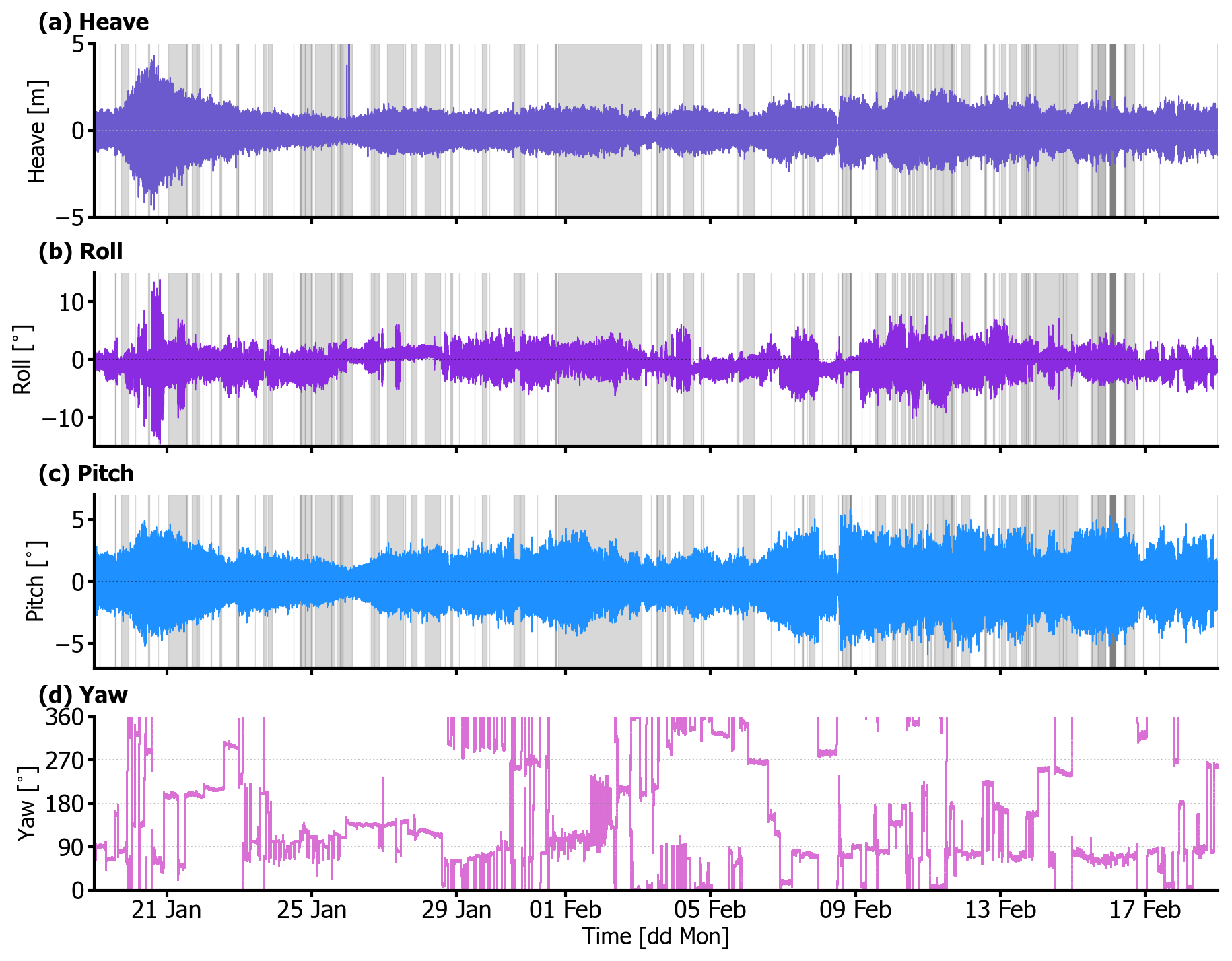
Figure 3Time series of (a) heave, (b) roll, (c) pitch, and (d) yaw of the R/V MS Merian MRU unit during the EUREC4A campaign, from 19 January to 19 February 2020. Grey areas represent the periods of time in which the stabilization platform did not work.
2.3 ARM AMF-2 stabilization platform
The stabilization platform from the US Atmospheric Radiation Measurement (ARM) program Mobile Facility 2 (AMF2) was deployed on the R/V MS Merian to reduce the impact of ship motions on the Doppler zenith pointing observations (Coulter and Martin, 2016). The system, built by Sarnicola Systems, is an active stabilization system; i.e., it compensates for the ship motions by adapting the position of the table surface correspondingly so that the radar stays in a zenith pointing position. It requires 120 V power and ethernet connection to a computer in a sealed container to be operational. A hydraulic power unit (HPU) (the cubic metal box on the right in Fig. 1a) must be within 600 cm of the table and weighs approximately 182 kg. The HPU supplies hydraulic fluid to manipulate the length of three legs positioned below the table's surface such that the table can compensate for a large range of roll and pitch angles of the ship. More information on the stabilization platform can be obtained at https://www.arm.gov/capabilities/instruments/s-table (last access: 23 December 2021). Ship and table motion are monitored by two roll–pitch sensors, one located on the ship deck and the other in the center of the table itself. A predictive computer routine uses these values to maintain the table in a geopotential level orientation at a constant height above the ship's surface. Thus the table compensates for the rotational motions around the long axis of the ship (roll) and the short axis of the ship (pitch). Stabilization platform data revealed that the table did not work for approximately 35 % of the time. The longest interval in which the stabilization platform was not working occurred between 1 and 5 February, when a connection cable was badly damaged and had to be exchanged. Around 17 February, we finally fixed the stabilization platform, and in the last 2 d the stabilization platform worked continuously. Overall, we encountered the roughest sea conditions at the beginning of the campaign, and we had relatively calm sea conditions afterwards (Fig. 3). It must be noted that the stabilization platform can compensate for the rotation of the ship, but it can not compensate for the vertical movements along the vertical axis (e.g., heave) and the translations which occur because the ship rotates around its center of mass while the instruments are located elsewhere (see Sect. 3).
2.4 Motion reference unit (MRU) and ship reference system
When deploying a radar on a ship, vertical velocity measurements have to be corrected for ship motions, i.e., roll, pitch, yaw, and heave (Fig. 3). Roll and pitch variations cause the radar beam to be off-zenith and vertical range to vary with time, heave variations in time cause a vertical velocity offset and the vertical range to vary with time, and the ship drift in the horizontal plane described by surge and sway may also have components in the direction of the radar beam if the radar is looking in any direction tilted from the vertical relative to ocean. In this work, we will not calculate the surge and sway motions because we assume them to be negligible compared to the other terms.
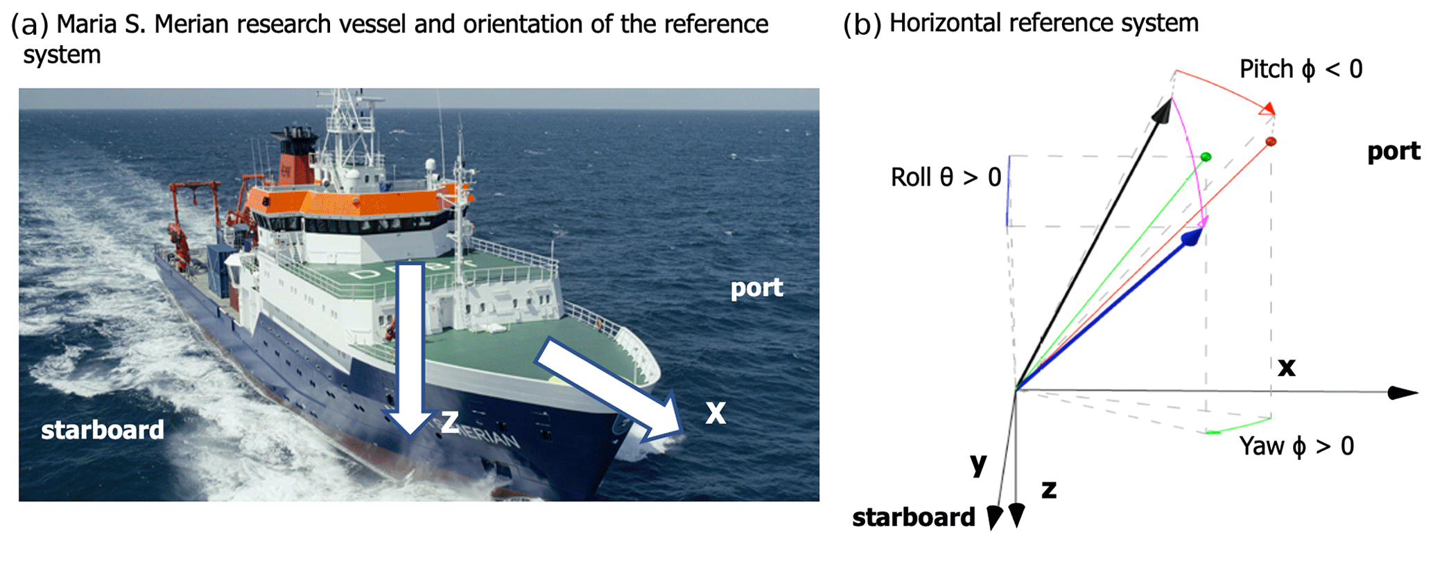
Figure 4(a) Port and starboard with respect to the R/V MS Merian. (b) Position of the radar and its tilting due to ship motions expressed in terms of roll, pitch, and yaw of the ship. The original position is represented by a black vector (arrow), and the position after the movement is given by a blue arrow. The angle representing the rotation from the initial to the final position is η, the angle between the blue and the black arrows. The roll, pitch, and yaw in which it can be decomposed are shown in blue, red, and green, respectively. The solid red and green lines ending in filled circles of the same color represent the vector position after undergoing the rotations due first to pitch and then to yaw. The application of the rotation with respect to roll would then bring the black array on the blue one. The sign with respect to the conventions indicated in the text is reported in the figure.
All rotation angles are measured by the motion reference unit (MRU) on the ship with a time resolution of 1 s. The MRU is a Kongsberg “Seapath 320” system manufactured by Kongsberg SeaTex AS. The sensor uses two single-frequency 12-channel GPS receivers for position and heading and provides roll, pitch, yaw, and heave with an accuracy of 0.03∘, 0.03∘, 0.075∘, and 0.05 m, respectively (from https://www.ldf.uni-hamburg.de/en/merian/technisches/dokumente-tech-merian/handbuch-merian-eng.pdf, last access: 23 December 2021). The MRU is mounted at the ship's center of gravity to clearly separate between translatory and rotational movements of the ship. As the radars are not at the ship's center of gravity, rotational movements of the ship lead to translation of the instruments. To calculate these movements, it is necessary to know the position of the instruments with respect to the MRU. They were determined as vectors in the ship's coordinate system as follows (Figs. 4 and 1c).
In the MRU sensor's conventions, roll angle is positive when port goes up, pitch angle is positive when bow goes up, and yaw angle is positive clockwise from the heading angle. The yaw of the ship is given as the angle clockwise from north and refers to the x axis of the ship system. Finally, the coordinate for heave is negative for upward directions. The angle η is the angle between the initial position of the radar r (black vector in Fig. 4) and its final position r′ (blue vector) after a given motion due to the ship; η can be decomposed in terms of roll θ, pitch ϕ, and yaw ψ (Fig. 4). The 35 % of the time in which the stabilization platform blocked itself in a random position is represented as grey areas in Fig. 3.
This section describes the corrections applied to the data to obtain the final reference dataset. Section 3.1 describes the drift problem in time between the radar and the ship clock that both radar datasets undergo. Synchronization of the two is thus necessary before applying any ship motion correction. Section 3.2 shows how to calculate the ship motion correction term for both radar datasets, and Sect. 3.3 assesses the correction algorithm. Finally, Sect. 3.4 shows how to filter interference for MRR-PRO data.
3.1 Tackling time drift between ship and radar time stamps
At the beginning of the campaign, we synchronized the ship and radar clock. However, the ship and radar clock cumulated a time lag ΔT that varies with time between 1 and 4 s. To calculate the time-varying ΔT, we use the heave rate time series and the time series of the mean Doppler velocity averaged over the cloudy range gates of each radar profile (see Sect. 3.3 for more details on why to use the heave rate time series). For stationary radars, i.e., radars not moving in time, the mean Doppler velocity (vd) measures the mean velocity of the hydrometeors in the radar volume with respect to the radar that results as superposition of the air motion and the sedimentation speed of the drops. The average of vd over the cloud geometrical thickness fluctuates around zero in non-precipitating regions, because the sedimentation speed of cloud droplets is negligible, and updrafts and downdrafts present in the cloudy column are averaged out. In precipitation regions instead (for example in Fig. 5 after 06:17:07 UTC), it becomes more and more negative, because of a larger and persistent downdraft. When the radar is moving (like on the ship), additionally tracks the radar motion (Fig. 5).
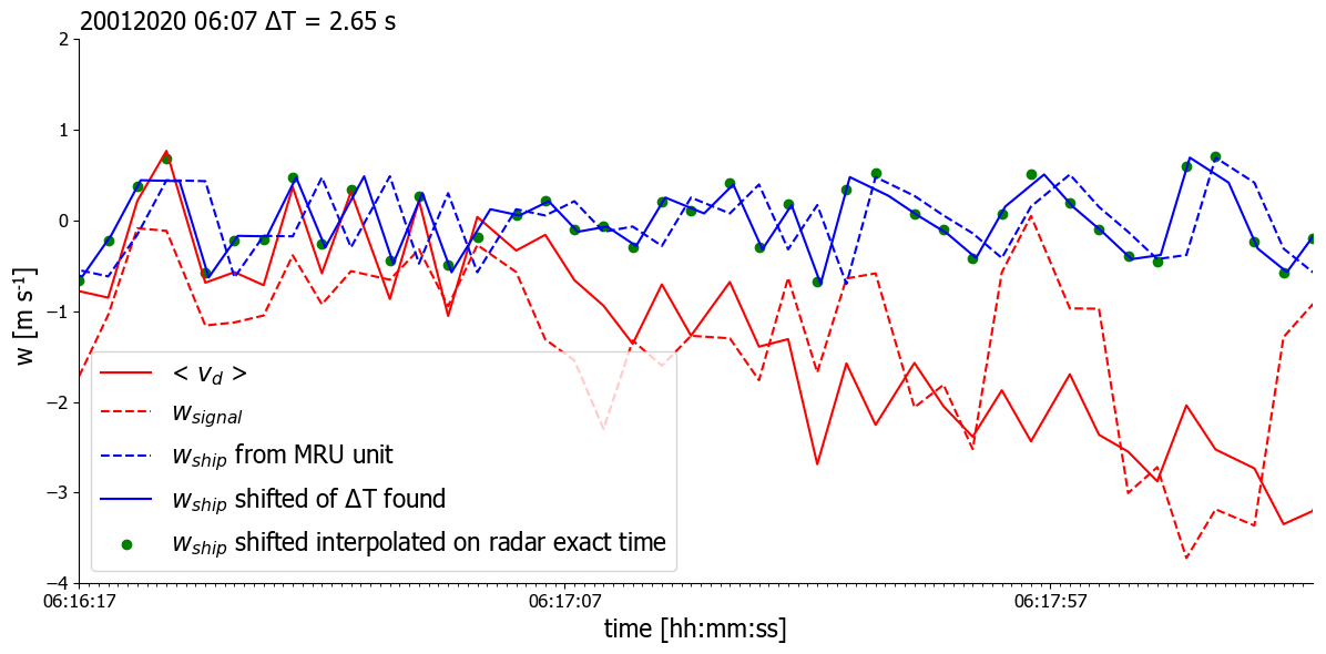
Figure 5Example of time shift application calculated to obtain the best matched correction for ship motion from the 20 January 2020 over 2 min between 6:16:17 and 6:17:57 UTC. The dashed blue line represents the vertical velocity measured by the ship wship. The dashed red line is the mean Doppler velocity recorded by the radar at 1230 m, while the solid red line represents , the mean Doppler velocity obtained by averaging together all cloudy pixels in each radar profile. The solid blue line represents the ship velocity after applying the time shift of ΔT=2.65 s, and the green dots represent the values of wship finally used for correcting for ship motion. They are obtained by cubic interpolation of the shifted ship velocity (solid blue line) on the radar time stamps. In fact, they correspond to the values of the red lines, as expected after interpolation. In the first 7 s of the time series, a short train of three waves is clearly visible that matches the radar observed mean Doppler velocity values much better after the time shift.
By comparing the heave rate (dashed blue line) and time series (solid red line in Fig. 5), we can derive the time lag ΔT. Cloud droplets have a vertical speed whyd. The ship moves vertically due to waves with wheave. To a first approximation, we can neglect additional contributions from the rotational movements of the ship (for the full vectorial equation see treatment in Sect. 3.2). The radar measures Doppler velocity vd with respect to the instrument on the ship; hence . Whereas whyd may vary with height due to up- and downdrafts in the cloud, wheave is the same within one time step for all range gates. We average over all cloudy range gates within one time step to get . By doing so we partly remove the turbulent variation in whyd, whereas wheave remains unaffected. From the ship's MRU we have a time series , whose time stamp might be shifted against the radar time series. We calculate the variance var(Δvd) of the difference Δvd between and over a time span of 10 min for different time shifts dt. By doing so we get
where . Ship movements wheave and whyd are not correlated; i.e., the covariance term should become zero. The equation then results in
For an optimal time shift dt, which we call ΔT, the variance of the difference dwheave should become minimal (close to zero), and accordingly var(Δvd) is minimal.
We then applied the resulting time lag ΔT to the ship data and interpolated this shifted series to the exact radar time, obtaining the best correction term for each time stamp. We iterated the procedure for every radar chirp sequence since they all have different time stamps. Only after matching the time series of data from the ship and data from the radar could we apply the ship motion correction.
3.2 Derivation of the ship motion's correction formula
In the following we will derive the equations to remove ship movements from the observed radar Doppler velocities with and without a working stabilization platform. The algorithm applies to both radars. The only difference is that while for the W-band radar the correction was applied to the mean Doppler velocity, for the MRR-PRO the whole Doppler spectrum is shifted by the correction. We will adopt bold notation for vectors, i.e., , where vi represents the components of the vector v along the various axes.
The ship's coordinate system is defined by a right-handed system with unit vectors , in direction of the bow, towards starboard, and perpendicular to the decks downwards (Fig. 4). With the ship moving in the waves, this coordinate system is rotated by roll and pitch angles. This rotation is described by a rotational matrix R (see Eq. C4 in Appendix C). By applying the R to unit vectors of the ship system, we get a coordinate system with pointing vertically downward in the direction of earth gravitational acceleration g and vectors and horizontally pointing in the direction of the ship's bow and starboard, respectively. We call this system the horizontal coordinate system (Fig. 4). is the pointing direction of the axis of the horizontal coordinate system and points downward.
The radar observes Doppler velocities relative to its own movement along its radar beam, and they are positive for movements away from the radar, i.e., upward for a vertical-pointing instrument. The Doppler velocity measured by the radar is the projection of the particle's velocity vector on the radar line of sight. Therefore, the component of the velocity vector of the hydrometeors wsignal measured by the radar is positive when hydrometeors move upwards. The pointing direction of the radar in the horizontal system is denoted as . During times when the stable table is working, it is ( pointing upwards, pointing downwards). The velocity observed by the radar is the relative velocity between hydrometeors (vhydr) and the movement of the radar (vradar) projected onto the pointing direction of the radar () that is
where all vectors are given in the horizontal coordinate system, and the dot represents the scalar product. The movement of the hydrometeors can be decomposed in the horizontal system into a component along the vertical axis and one in the horizontal plane:
where the term vhydr,s is the hydrometeor fall speed in the horizontal reference system (z component), and vwind,s is the horizontal wind vector in the horizontal reference system (for the derivation, see Appendix B). Hence, we get
Now solving Eq. (4) for vhydr,s that is the hydrometeors' fall speed in the horizontal reference system, we get
In the case of a working stabilization platform, the radar pointing vector is exactly upwards, and accordingly the scalar product is equal to −1 as is pointing downwards. In the limit of a non-moving ship we get , where the opposite sign is given by the fact that the ship reference system has an opposite z direction to the one in the radar convention. Finally in the common definition with falling hydrometeors having negative velocities, we get
The pointing direction of the radar in Eq. (5) changes depending on whether the stabilization platform is working or not.
-
If the stabilization platform is working perfectly, we assume that .
-
If the stabilization platform is not working, the pointing vector of the radar moves with the ship coordinate system. Accordingly has to be rotated with the ship's rotation matrix R in the horizontal system, and we get . The table typically got stuck at an arbitrary position, and thus the radar points in an arbitrary direction. We reconstruct this direction by taking roll and pitch at time t0 just before the table got stuck and assuming that the radar was pointing vertically at this moment. Orientation of the radar in the ship system is thus , which then translates to , where R−1 is the inverse matrix of R (see Appendices C and D for more details).
The velocity vector vradar in Eq. (2) is composed of various contributions to the motion:
where the velocities that add up to the radar movement are as follows.
-
The translation velocity vector vtrans depends on the translation movements of the ship: heave, surge, and sway (we neglect the surge and sway contribution), and it is given by (see Appendix E for the derivation).
-
The course velocity vector vcourse is due to the travel of the ship along its course, and it is given by , where ψ is the yaw and vs is the magnitude of the ship velocity vector (see Appendix E for the derivation).
-
The rotation velocity vector vrot describes the movement due to the rotation of the ship (roll, pitch, yaw) and the fact that the instruments are not deployed in the center of rotation but at distances rMRR-PRO and rW-band from it. Its expression is (Appendix C for the derivation of the full expression).
3.3 Application of the correction and additional smoothing
When the table is working and the radar is pointing vertically, all horizontal vector components vanish, and the expression of the corrected hydrometeor velocity reduces to
where and are the z components of the vectors vtrans and vrot. In this case, for calculating the velocity terms we need roll, pitch, and heave rate. All these data are provided by the ship navigation system. Angles of roll and pitch are necessary because the rotation of the ship moves the radar vertically. Course (yaw and speed) is not necessary as it is a horizontal component not seen by the vertical-looking radar.
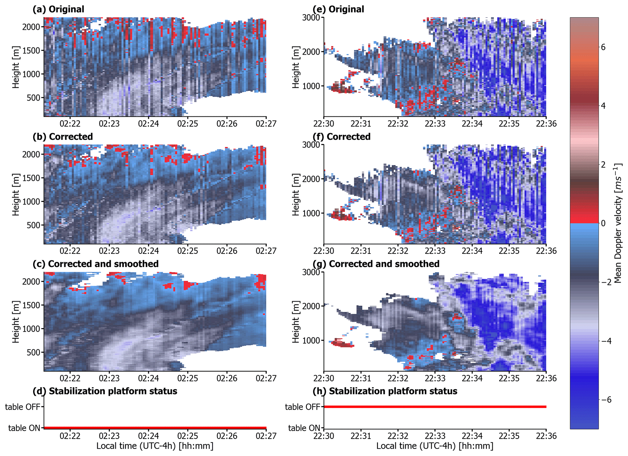
Figure 6On the left is an example of the ship motion correction algorithm applied when the stabilization platform was working, on 20 January 2020 from 02:21 to 02:27 LT (UTC−4h) for the W-band radar data with de-aliasing applied: (a) original mean Doppler velocity field without any correction algorithm applied, (b) mean Doppler velocity after application of the correction from ship motions, (c) mean Doppler velocity after application of correction from ship motions and smoothing (running mean over 9 s), and (d) status of the stabilization platform. On the right is another example when the stabilization platform did not work, on 12 February 2020 between 22:30 and 22:36 LT: (e) original mean Doppler velocity field without any correction algorithm applied, (f) mean Doppler velocity after application of the correction from ship motions, (g) mean Doppler velocity after application of correction from ship motions and smoothing (running mean over 9 s), and (h) status of the stabilization platform.
When the table is not working, the pointing vector of the radar is not vertical most of the time and may have a horizontal component (scalar products of with horizontal vector components do not vanish). Accordingly, course of the ship and horizontal wind may contribute to the signal. We therefore need the additional parameters yaw and speed of the ship and the horizontal wind above. The first two are provided by the ship's navigation system. For the wind we used the output of dedicated ICON simulations run (Daniel Klocke, personal communication, 2020) over the EUREC4A domain to extract the horizontal wind profiles at the closest time and place of the ship, corresponding to the time when the table was not working. This type of correction affected 35 % of the total measurement time. The low time resolution of the model output compared to the observations made this correction less accurate than the one applied for the 65 % of the data in which the stabilization platform worked correctly.
An example of the application of the correction for ship motions when the stabilization platform is working is visible in Fig. 6a–d, for the case of 20 February 2020 between 02:22 and 02:27 LT (local time), with especially strong waves (compare with Fig. 3).
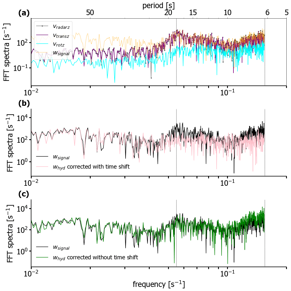
Figure 7(a) Fast Fourier transform (FFT) of the vertical component of vradar and of its translational (purple) and rotational (cyan) components for 1 h of data collected at a cloudy range gate located at 1605 m from the radar (all terms along z in Eq. 7). The FFT highlights two main wave periods around 6 and 17 s, indicated by dashed vertical lines. In the total radar velocity along z (black dotted line), the contribution of the rotational component is minor compared to the contribution of the translational component (heave). (b) Comparison of the FFT of the uncorrected mean Doppler velocity (black) measured by the radar and of the FFTs of the corrected mean Doppler velocity with time shift applied. The two main wave peaks disappeared in the corrected signal (pink line). (c) Same as the middle panel, but with the corrected mean Doppler velocity calculated without applying the time shift. In this case, the wave frequencies are not removed from the corrected signal (green line).
When comparing the original (Fig. 6a) to the corrected mean Doppler velocity field (Fig. 6b), one can quickly notice that many of the intense and frequent vertical bars disappear, providing a more homogeneous and continuous field. However, the correction cannot entirely remove the disturbances, as shown in Fig. 6b by some visible vertical bars remaining despite the correction. Some possible reasons for the mismatch observed are the distance between the MRU sensor and the radar equipment, especially considering that we measured the radar equipment's position by hand. We also assume that the stabilization platform keeps the radar perfectly in zenith, but it is hard to quantify the accuracy of such a hypothesis since a small error in the zenith alignment can produce disturbances. Moreover, the time lag quantification ΔT can be unprecise due to the reinitialization of the chirp generator of the W-band radar. Such time is random and adds an unknown uncertainty to the time stamps assigned to the measurements. Finally, the coarse temporal resolution of the MRU data makes an interpolation to the radar data necessary. Figure 5 nicely shows the rapidly changing wship, which misses the real minima and maxima due to its coarse temporal resolution, making an interpolation challenging. We applied a running mean over three time stamps (i.e., over a 9 s time interval) to account for these limitations (Fig. 6c). The final signal obtained shows an almost continuous field in mean Doppler velocity.
Figure 6e–g show the correction performance when the table did not work, on 12 February between 22:30 and 22:36 LT. Even if the final smoothing (Fig. 6g) improves the vd pattern compared to the field obtained when applying the correction algorithm only (Fig. 6f), overall the performance is worse than in Fig. 6a–c, and vertical stripes are markedly visible in all fields. We also applied the time shift and the ship motion correction to the MRR-PRO data, obtaining similar results as will be shown in Sect. 3.4.
Figure 7 for 1 h shows the impact of the time matching and of the correction applied to the signal in the frequency space. The heave rate is the main contributor to the vertical motion of the radar (Fig. 7a), as described by looking at a cloudy range gate. The rotational components are approximately 1 order of magnitude smaller because the instruments are not too far from the center of mass of the ship, and the rotation of the ship does not move the instrument much along the vertical. For this reason, it represents the vertical velocity of the ship due to the waves, as previously stated. The frequencies of the waves at approximately 6 and 17 s (highlighted by the vertical dashed bars in Fig. 7) are visibly removed in the FFT spectra of the corrected mean Doppler velocity only if the time shift is applied (compare Fig. 7b and c). Finally, the increase in the spectra towards the Nyquist frequency, between 0.1 and 0.5 Hz, indicates that there are higher frequencies above 0.5 Hz, folded back into this interval. Such frequencies do play a role that is not resolved by MRU or by the radar itself. The final smoothing over the 9 s time window removes the high-frequency components, and it is thus crucial to obtain a better signal-to-noise ratio. However, the 9 s smoothing degrades the average horizontal resolution of the Vhyd,mean by a factor of 9. For an average ship speed of 3 m s−1, the resolution would change from 3 to 27 m, resulting in a slightly higher resolution than the vertical 30 m one. However, daily maximum speeds for the ship can also reach 9 m s−1, thus producing a coarser resolution.
3.4 Removal of interference patterns and correction for ship motions for MRR-PRO dataset
The MRR-PRO electronics interfered with the ship instrumentation and with the stabilization platform electronics during the whole campaign. To be able to use the data collected, we removed the interference patterns using a noise removal mask. The interference draws periodical disturbances with peak intensity decreasing with height. Since the interference peaks are larger than the mean noise level calculated using the Hildebrand–Sekhon method by the manufacturer's processing (Hildebrand and Sekhon, 1974), multiple small peaks appear in the MRR-PRO spectra. The mean Doppler velocity and the spectral width of such noise spectra are random, depending on which noise peak is the highest (Fig. A1).
The MRR-PRO dataset produced by the software of the manufacturer is initially processed with the MRR-PRO post-processing tool (Garcia-Benadí et al., 2021). The algorithm allows us to obtain de-aliased Doppler spectra over a physically realistic Doppler velocity range. For data with 5 or 10 s integration time, this tool is sufficient to remove the interference pattern. No ship motion correction can be applied to those data because their integration time is larger than or similar to the typical wave period (see Fig. 7a), and Doppler variations due to heave motions are smoothed out. We resampled the data collected from 19 to 25 January 2020 with 5 s to 10 s integration time, to reduce the impact of ship motions completely.
The post-processing of the data collected with 1 s integration time, i.e., from 25 January to 19 February 2020, is more complex. For the 1 s resolution data, the tool from Garcia-Benadí et al. (2021) cannot remove the interference patterns as it did for the 10 s integration time dataset. Hence, to obtain Doppler spectra without interference, we applied a noise removal mask (interference filter in Fig. 8) based on specific conditions.
-
We calculated for each spectrum the prominence of all its spectrum peaks, i.e., each peak's ability to stand out from the surrounding baseline of the signal. Then, we derived the difference between the maximum and minimum prominence and calculated their difference (ΔP). The difference is tiny for spectra containing only interference patterns and no signal from hydrometeors, while it is significantly larger for a Doppler spectrum detecting hydrometeor backscattering (see for reference in Fig. A1). Spectra affected by interference patterns were removed by selecting spectra with ΔP>1 mm6mm−3, where the threshold value of 1 was determined empirically.
-
In addition, we posed a condition on the spatial continuity of mean Doppler velocity (mdv) in the lowest 600 m. The mdv obtained from spectra affected by interference shows very large random absolute values. Doppler spectra detecting hydrometeors produce continuous mdv field in space. We discarded all profiles where the difference of consecutive mdv values along the profile shows more than eight abrupt peaks (threshold decided empirically).
-
We apply a spatial filtering to remove spurious noisy pixels: the filters exclude all pixels where ΔP>1 that have fewer than three adjacent neighbors fulfilling the same condition.
It is almost impossible to distinguish the signal due to hydrometeors from the one due to interference in the reflectivity field Ze of the original dataset. However, after applying the noise removal mask the hydrometeor signal becomes clearly visible (Fig. 8a and b). The time correction (see Sect. 3.1) and post-processing tool from Garcia-Benadí et al. (2021) were then applied to remove the time lag ΔT and de-alias and obtain a physically realistic Doppler velocity range for all Doppler spectra above the noise level (Anti-aliasing in Fig. 8). Then, ship motion correction derived with the calculations presented in section 3.2 is applied and all the main MRR-PRO variables of interest are derived from the corrected Doppler spectra. Figure 8d shows a hook rain structure visible, possibly caused by downdraft wind mixing. The vortex structure was not visible in the original data (Fig. 8c) and emerged from the noise after applying the correction on the mean Doppler velocity field.
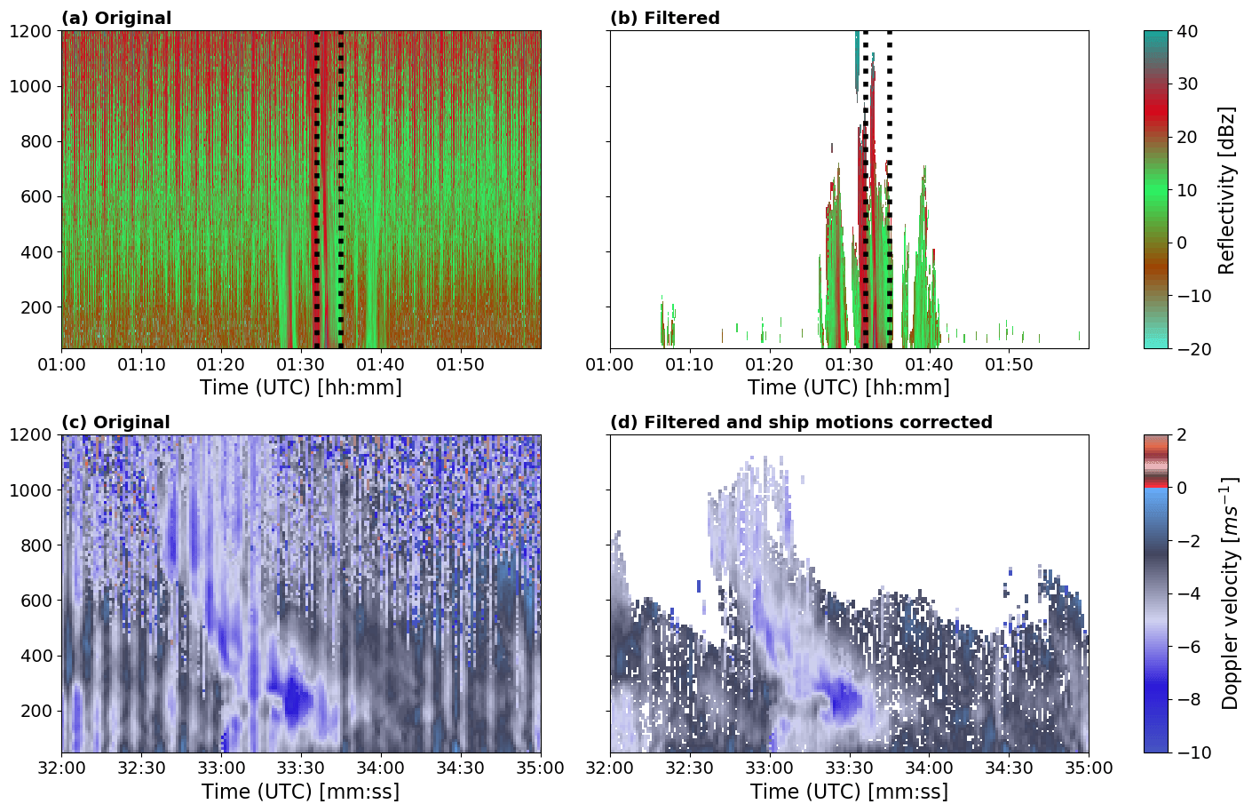
Figure 8(a) MRR-PRO attenuated reflectivity on 13 February 2020 at 01:00 UTC after manufacturer processing, without any additional interference filtering or ship motion correction. (b) Same as (a), but with the noise removal mask applied. (c) MRR-PRO mean Doppler velocity without any correction over a 2 min time interval selected from the time interval shown in (a) between 01:32 and 01:35 UTC and (b) and highlighted with dashed black lines. Vertical stripe structures are visible due to ship motions. (d) Same as (c) but with interference removed and time shift and ship motion corrections applied to the data. The striped structure present in (c) almost entirely disappeared.
To give an overview of the meteorological conditions encountered on each of the 32 d of campaign, Table 3 lists the daily mean atmospheric temperature (T2m), rain rate (RR), liquid water path (LWP), relative humidity (RH), and pressure (P) for each day of the campaign. They are collected at the radar base, which is approximately 20 m a.s.l. (above sea level).
Table 3Daily mean values of the main surface variables observed on the MS Merian during the EUREC4A campaign: T2m is the air temperature 2 m above the radar base, which is approximately 20 m a.s.l. (above sea level), RR is the rain rate. The liquid water path (LWP) is derived from the collocated 89 GHz channel microwave radiometer, and RH and P are the relative humidity and air pressure from a weather station positioned next to the radar equipment.
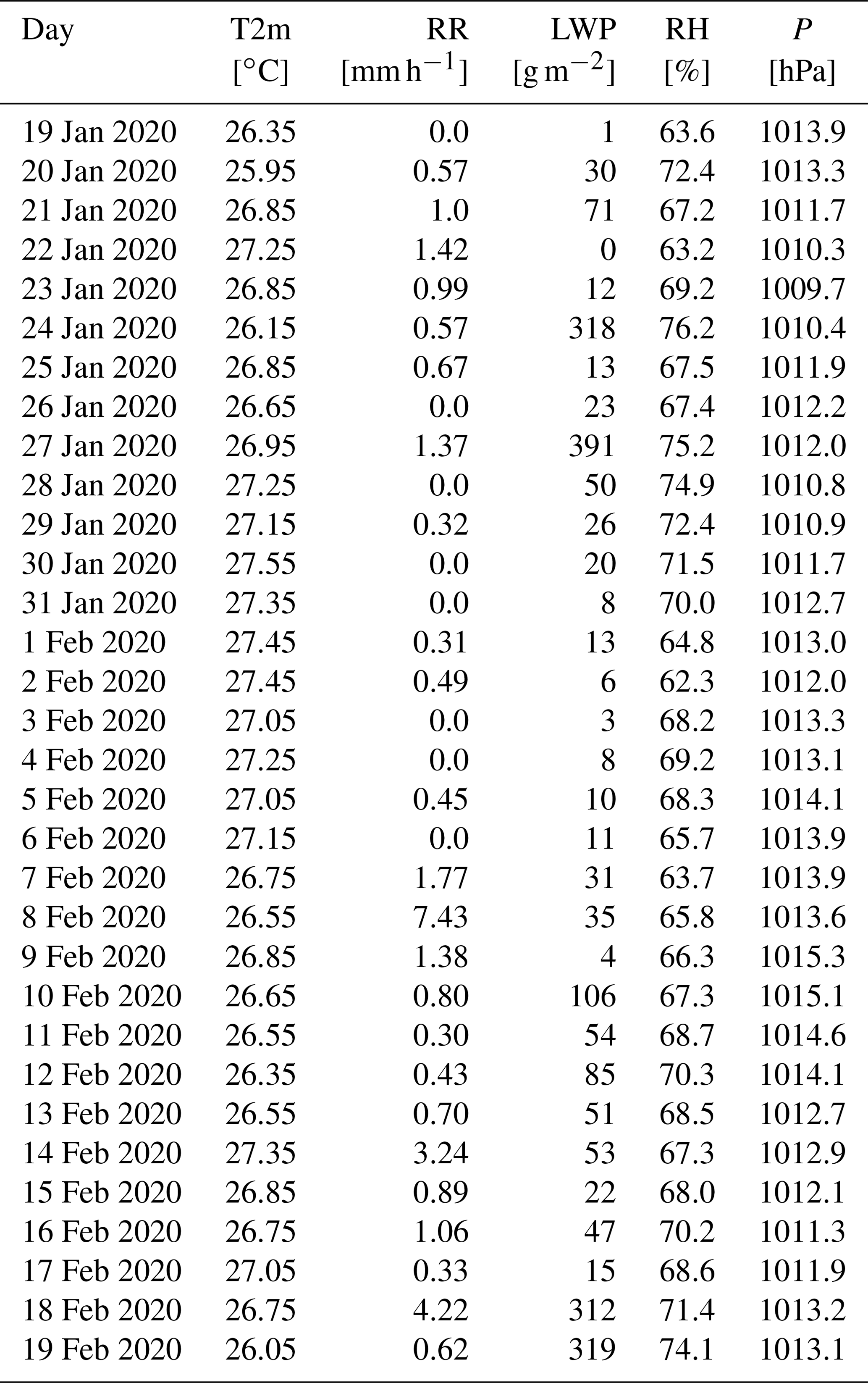
Figure 9 shows that the vast majority of the encountered liquid clouds have a LWP smaller than 100 g m−2, with a median value of 11 g m−2 in agreement with Schnitt et al. (2017), who sampled the region between 10 and 20∘ N and −40 and −60∘ W in December 2013. Noise and gain drifts in the passive channel of the radar lead to positive LWP retrieved values even in clear-sky conditions. These data have a median and standard deviation of 1.2 and 5.4 g m−2, respectively, which are within the retrieval uncertainty (about 30 g m−2). The standard deviation of the clear-sky distribution can be considered a sort of uncertainty of the LWP values retrieved with the neural network algorithm and can be used to correct the LWP values, as done in Jacob et al. (2019).
We compared the obtained IWV values with the IWV retrieved from GNSS by Bosser et al. (2021). The mean of the IWV retrieved from W-band radar single-channel retrieval is 31.7 kg m−2, the median is 32.3 kg m−2, and the standard deviation of the distribution is 5.15 kg m−2. The bias between the mean value of the IWV distribution from W-band and the IWV distribution from GNSS is 3.4 kg m−2, which is consistent with the bias estimated with ground-based GNSS stations reported in Fig. 9 of Bosser et al. (2021). The spread between the GNSS and the radar-derived values of IWV can be due to the strongly varying bias component that affects the GNSS IWV estimations from MS Merian (Bosser et al., 2021), as well as to limitations in the IWV single-channel retrieval.

Figure 9LWP distribution for cloudy (blue) and clear-sky (red) conditions, for the whole campaign.
To show the full potential of the collected radar dataset, we display one case study of an extended precipitating cloud field occurring on 12 February 2020 from 15:00 to 17:00 UTC in the trade wind alley at about 13.5∘ N and 57∘ W. On that date, the ship encountered a cloud system identifiable as a flower type (Bony et al., 2020) using the corrected reflectances from Moderate Resolution Imaging Spectroradiometer (MODIS) TERRA (Platnick et al., 2003), with a diameter between 200 and 250 km that generated precipitation during the afternoon (Fig. 10c). When comparing the signals observed by the W-band radar (Fig. 10a) and the MRR-PRO (Fig. 10b), the different sensitivities of the two instruments become evident: while the W-band is capable of detecting cloud and precipitating hydrometeors, the MRR-PRO is sensitive to larger raindrops only. The interference patterns reduced the ability of the MRR-PRO to detect precipitation in a way that it is difficult to quantify. The W-band radar system collected echoes in the first 2200 m, showing the complex internal structure of the clouds. The cloud base detected from the W-band radar ranges between 750 and 1250 m and does not exactly correspond with the lifting condensation level (LCL) values (black solid line in Fig. 10a and b) obtained for this case, while in non-precipitating conditions LCL is higher. Cloud top ranged between 1700 and 2100 m.
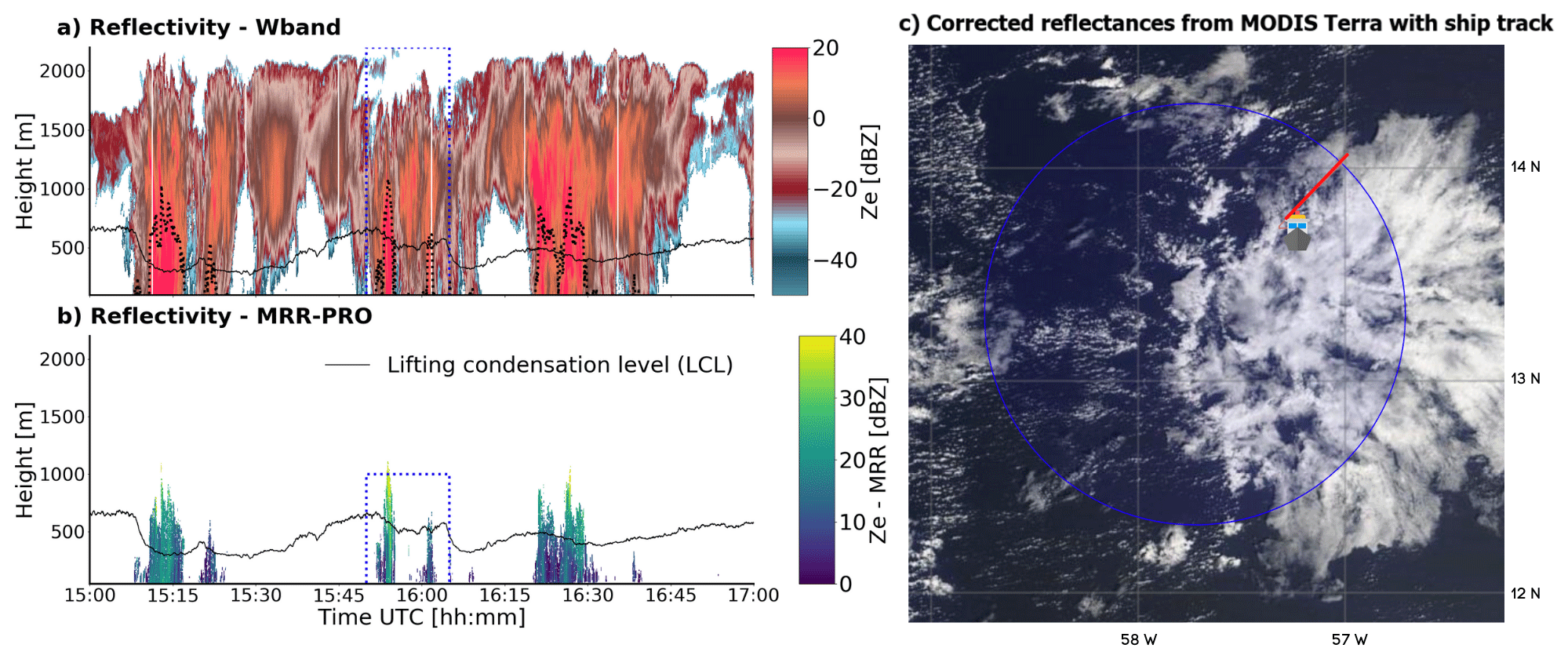
Figure 10Overview of the selected case study of 12 February 2020 between 15:00 and 17:00 UTC: (a) radar reflectivity from W-band radar. The black solid line represents the lifting condensation level calculated using the surface variables, while the black dotted line shows the highest detected signal from the MRR-PRO. The red dashed box represents the area shown in Fig. 11. (b) Attenuated reflectivity from MRR-PRO. (c) Ship track on top of the corrected reflectance from MODIS Terra, displaying the flower cloud occurring in the area. The corrected reflectance from MODIS is a product that uses the bands 3 (479 nm, red), 6 (1652 nm, green), and 7 (2155 nm, blue) produced in near-real time (NRT) to provide natural-looking images. The blue circle represents the orbit of the HALO aircraft. The image was taken at 16:03 UTC. Source: https://observations.ipsl.fr/aeris/eurec4a/Leaflet/index.html (last access: 23 December 2021).
The high-vertical-resolution mode for the W-band radar (7 m up to 1230 and 9 m from 1230 to 3000 m) detected distinctive features in the radar moments (Fig. 11a–d). Filaments of higher reflectivity between 15:53 and 15:55 UTC at around 800 m (Fig. 11a) suggest a correlation of the size of the drops with air motions; Fig. 11b displays clear areas in the cloud where larger mean Doppler velocities are associated with heavy rain. The spectral width field (Fig. 11c) also benefits from the high temporal and spatial resolution. It shows patterns that suggest a correlation between large reflectivities and mean Doppler velocity values as well as large spectral width values. Finally, the skewness field shows patches of positive and negative skewness emerging from the noise. Further analysis of the Doppler spectra in precipitation is necessary to interpret these patches and exploit the skewness signatures (Acquistapace et al., 2019).
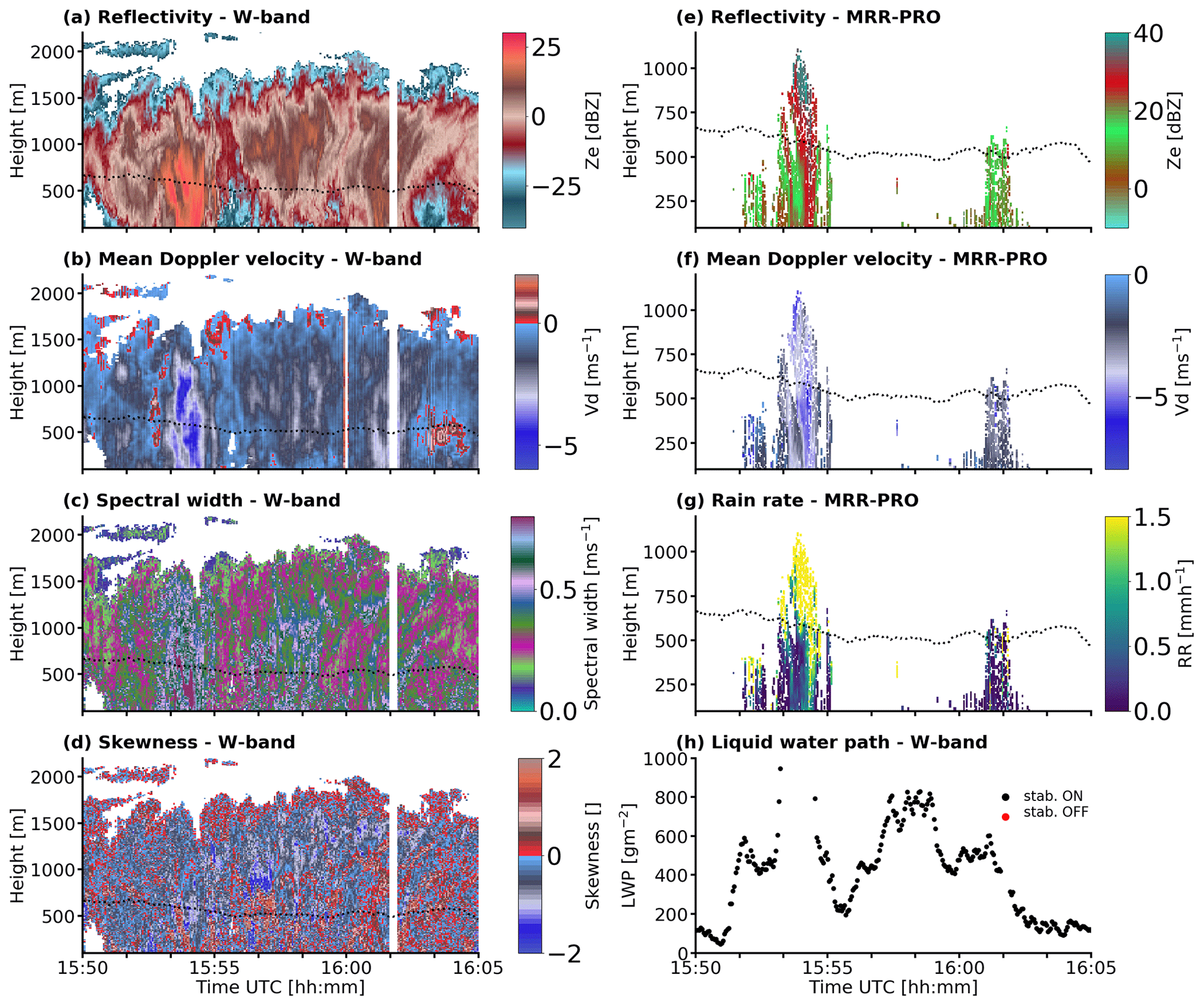
Figure 11Details of the case study shown in Fig. 10 for W-band variables (a) reflectivity, (b) mean Doppler velocity, (c) spectral width, and (d) skewness and for MRR-PRO variables (e) attenuated reflectivity, (f) mean Doppler velocity, and (g) spectral width. LWP and stabilization platform status are displayed in (h).
Also, for the MRR-PRO, the high vertical and time resolution allowed us to reveal relevant structures in the lower precipitation field. Despite the small gaps caused by the filtering of the interference, the reflectivity (Fig. 11e) shows a decrease in the Ze values with decreasing altitude possibly due to evaporation and/or shear. The case study highlights a large variability of fall speeds in the lowest 300 m, possibly connected with sub-cloud layer dynamics. The fall speed field can also trace such dynamics, like the vortex structure in Fig. 8d. Also, the rainfall rate shows a substantial decrease as rain approaches the ground during the selected case study (Fig. 11g). During the case study the stabilization platform worked continuously and the LWP registered high values and saturated (LWP > 1000 g m−2) under rainy conditions. Note that values above 1000 g m−2 should not be considered reliable because of contamination due to rain.
The data presented in this paper can be accessed at the AERIS repository and in the ARM database in NetCDF format, under https://doi.org/10.25326/235 (Acquistapace et al., 2021c). This DOI was assigned to the new version of the dataset, produced after fixing a bug in the standard post-processing script and correcting the LWP neural network dataset. In the dataset the following applies.
-
Technical radar variables were removed and stored in hourly technical files that can be accessed upon email request to the paper's corresponding author.
-
A Doppler velocity variable has been added to facilitate the usage of the Doppler spectrum variable.
-
A compact data version (including radar moments and geolocation) has been produced following CF conventions. The data are included in the Eurec4a book “How to EUREC4A”, which is an online and interactive Jupyter book (Jupyter is an interactive development environment supporting several programming languages; https://jupyter.org, jupyter, 2021). Data can be accessed via the intake catalog (https://github.com/eurec4a/eurec4a-intake, GitHub, 2021). The book and the intake catalog are living documents, continuously updated and developed further by the EUREC4A community. More details can be found in the section Accessing EUREC4A's HALO data of Konow et al. (2021). Some example codes on how to read the data and plot basic quantities are available for users. More support will be added here in the future.
An auxiliary dataset used for correcting for ship motions can be found at https://doi.org/10.25326/156 (Acquistapace et al., 2021b). together with the outdated version of the radar data.
The MRR-PRO data can be accessed at the AERIS repository and in the ARM databases (https://doi.org/10.25326/233) (Acquistapace et al., 2021a). Data are organized in daily NetCDF files. Also, this dataset follows CF conventions and is included in the EUREC4A intake catalog with example codes for basic operations with the data.
Finally, the code used for post-processing the W-band radar data is published on GitHub (https://github.com/ClauClouds/w-radar, Bravo Aranda et al., 2021). The post-processing software for MRR-PRO data is published in Garcia-Benadí et al. (2021). The code for ship motion correction and interference filtering and for deriving the plots of the paper can be accessed at Zenodo https://doi.org/10.5281/zenodo.5714474 (Acquistapace et al., 2021d). All the data are visualized in hourly and daily plots on the quicklook browser https://bit.ly/3xLkb9b (Acquistapace and Pschera, 2021). For improving the data visualization (Zeller and Rogers, 2020), we created color palettes using the Colorgorical tool (Gramazio et al., 2017), and we used them for all plots of the quicklook browser as well as for many of the graphics of this publication.
As underlined in the introduction, we experienced various challenges deploying active remote sensing instruments on the MS Merian research vessel. For encouraging and facilitating future deployments on ships, we collected some issues we encountered that future technological developments could solve.
The ship motion correction algorithm described here has also been tested on the radar data collected on the Meteor research vessel, where the ship navigation system data used 0.1 s (10 Hz) time resolution. We noticed that increasing the time resolution of the ship position data from 1 to 10 Hz is beneficial for the ship motion correction. Spectral analysis of the data from MS Merian indicates that there are components of the ship movement at frequencies above 0.5 Hz which had to be filtered out by a simple gliding average smoothing operator. We therefore recommend using 10 Hz for future campaigns.
A significant limitation to the exactness of the correction came from the need to synchronize the radar clocks with the GPS time from the ship. This is necessary to assign the right correction to be used for the measurements. The synchronization problem is a well-known issue for aircraft measurements, and more research is needed to tackle this point. At least for ship purposes, a possible solution could come from including a high-resolution sensor in the radar that can tell the radar inclination and heave for each radar partial chirp sequence time stamp with high precision. Currently W-band radar position data (inclination and elevation) are provided with the time resolution of the total sampling time, which is approximately 3 s and is too poor for an effective correction of ship motions.
Finally, we strongly recommend a preliminary test phase to the campaign, as we did in this work. The time spent before the campaign in testing the instruments allowed us to take care and solve small details that could have strongly affected the measurement quality, like the vibration of the pole or the best setup for the computer connections on board the R/V. We experienced interference problems on the ship. Interference is always hard to detect and to solve, but we recommend making some test measurements with all instruments and checking the raw data obtained. In our case, the MRR-PRO interference was not visible on the quicklooks of the control system, but it significantly impacted the observations. In a test phase, interference could be tackled and possibly solved.
This paper presents the W-band and MRR-PRO dataset collected on the MS Merian research vessel during the EUREC4A campaign between 19 January and 19 February 2020. We installed and operated two radars on the stabilization platform deployed on the ship with the collaboration of the ARM AMF2. The suite of instruments constituted an advanced setup for studying the precipitation life cycle in the tropical region and the first deployment of Doppler instrumentation on the R/V MS Merian. The ship sampled a broad oceanic region between 6 to 13.8∘ N and 60 to 51∘ W. The data collected provide a precious characterization of the trade region and the transition from the trades to the intertropical convergence zone. The ship sampled some mesoscale oceanic eddies, which are circular fronts of sea surface temperature anomalies caused by oceanic turbulence, locally impacting near-surface wind, cloud properties, and rainfall (Frenger et al., 2013). The collected observations will provide vital information to understand the impact of sea surface heterogeneities on the marine boundary layer.
We developed an algorithm to correct the Doppler observations from ship motions and successfully applied it to the W-band dataset. The algorithm initially calculated the time shift between the radar time stamps and the ship navigation system time to identify the radar position with respect to the motion reference unit as best as possible. It then applies the correction term to the mean Doppler velocity. For the MRR-PRO data, in addition to the ship motion correction algorithm, we also developed advanced post-processing techniques to filter out interference problems between the MRR-PRO and the stabilization platform. We first removed the interference pattern, and then we applied the correction directly to the Doppler spectra. Then, we used the standard post-processing to derive the moments and the other rain-related variables from the corrected Doppler spectra.
The corrected fields remove most of the typical striped pattern due to heave motion in the mean Doppler velocity (W-band) and fall speed (MRR-PRO) that ship motions cause to Doppler measurements. The correction for ship motion was applied to the entire dataset. However, for 35 % of the data, the stabilization platform did not work. We corrected this data subset using the horizontal wind profile extracted from NWP ICON-LEM model runs and horizontal ship velocity.
A unique feature of the dataset is the high temporal and vertical resolution: the time resolution is 3 s (W-band) and 1 s (MRR-PRO). Below 3000 m, i.e., where most of the cumulus liquid clouds develop, the range resolution of the W-band is 9 or 7 m, while that of the MRR-PRO is 10 m. The profiles of the W-band radar moments detected with unprecedented detail showed characteristic patterns that will be explored in future works, especially for what concerns the spectral width and skewness. MRR-PRO variables like the fall speed contain important detailed information on the dynamical evolution of the rain in the sub-cloud layer and its interaction with the dynamics. We exploited the passive 89 GHz channel available on the W-band radar to retrieve LWP in cloudy conditions and IWV in clear-sky situations. The LWP retrieval is a neural network retrieval provided by the radar manufacturer, while the IWV is derived from a single-channel quadratic regression between the 89 GHz brightness temperatures obtained in clear sky and the IWV measured by the radiosoundings launched at the exact times. We assessed the IWV retrieval by comparing it to the IWV estimations obtained by GNSS (Bosser et al., 2021). We found a bias of 3.4 kg m−2, in agreement with what was reported in Bosser et al. (2021).
The high resolution of the collected datasets and the possibility of synergies with the other instrumentation on board, i.e., Raman lidar, wind lidar, and cloud kite, make the described observations a benchmark dataset for future analysis as model studies and evaluations, comparing satellite retrievals and process studies. We made the data public and accessible on the AERIS and the ARM database platforms to achieve these purposes. Moreover, we also made the data accessible online via the EUREC4A intake catalog, and hourly and daily quicklooks are available online for browsing into the data.
Future work will focus on improving the quality of the correction: when the wind-lidar-corrected dataset from MS Merian is published, it will provide horizontal wind profiles for the entire campaign and thus allow us to obtain a better correction for the 35 % of the dataset collected when the stabilization platform did not work.
This appendix describes the neural network retrieval developed to retrieve LWP from the single passive channel at 89 GHz of the W-band radar, exploiting radiosoundings launched in the region of the campaign. The dataset consisted of the three radiosonde stations collocated in Grantley Adams International Airport (Barbados), the international airport of “Le raizet” (Guadeloupe), and Piarco International Airport (Trinidad) and the one location from the ERA-Interim reanalysis (see Table A1). All available profiles from January 1994 to December 2016 were used. In total, there were 41 588 profiles. We used 29 111 (70 %) randomly chosen profiles for the ANN training and 10 % of the dataset for the validation. We used the remaining 20 % for the retrieval evaluation (test dataset). For each profile, we calculated the LWP following Löhnert and Crewell (2003). A radiative transfer model was used to simulate TB values at 89 GHz. The absorption of oxygen and water vapor was calculated according to Rosenkranz (Rosenkranz, 1998, 1999). The absorption by liquid water was calculated using the Rayleigh scattering approximation and the model from Liebe et al. (1991) and Liebe et al. (1993).
We used as input variables for the ANN training the simulated brightness temperatures (TB), day of the year, near-surface temperature, relative humidity, and pressure. The values of temperature, relative humidity, and pressure closest to the surface were taken from profiles. The calculated LWP was used as the target variable. The input and the target variables were normalized using the min–max function. The ANN consists of two layers: a hidden layer with five neurons and an output layer with one neuron. The hyperbolic tangent is used as an activation function for all neurons. The standard error backpropagation algorithm was used for the training. After the training, we evaluated the retrieval using the test dataset. The retrieval root-mean-square error (RMSE) is 33 g m−2. During the radar operation, the ANN uses TBs measured by the passive channel and measurements of the surface temperature, relative humidity, and pressure from the weather station.
Table A1Information about the radiosonde stations (data taken from https://ruc.noaa.gov/raobs/intl/, last access: 23 December 2021) and the ERA-Interim data point used for the retrieval of LWP using neural networks.

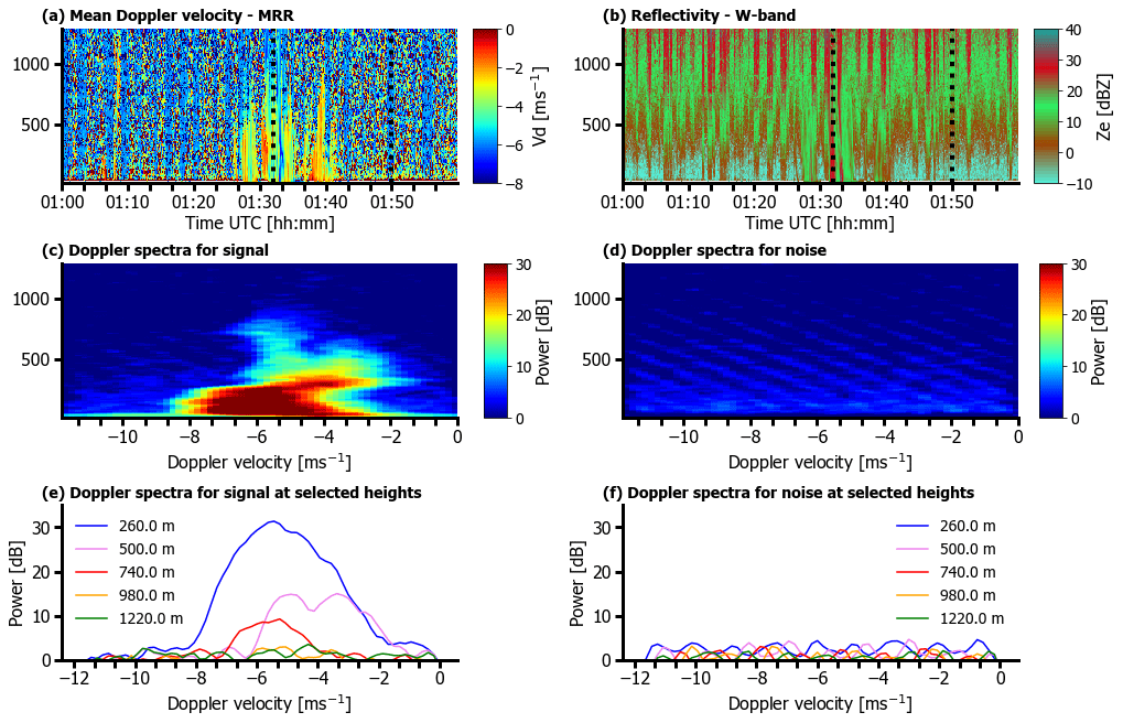
Figure A1Interference in the MRR-PRO data: (a) mean Doppler velocity for one selected hour. The black vertical lines correspond to the selected times for plotting the spectra shown in panels (c)–(f). (b) Same for reflectivity. (c) Height spectrogram of MRR-PRO Doppler spectra collected at 01:33:00 UTC during rain. (d) Same for Doppler spectra collected at 01:50:00 UTC, in the noise. (e) Doppler spectra collected along the vertical selected profile for rain at various heights. (f) Doppler spectra collected along the vertical selected profile for noise, at various heights.
In the Earth reference system, the horizontal wind vector in absolute coordinates is given with the zonal component towards the east and the meridional component towards north, and it represents the direction where the wind is coming from. If it has a speed vwind,E and a direction indicated by α clockwise from north, it can be written in Cartesian coordinates as
After applying the rotational matrix of ship motions, the horizontal coordinate system (see Fig. 4) has
-
an x axis to the yaw of the ship, horizontal, perpendicular to the gravity acceleration g;
-
a y axis to the starboard of the ship, right side, horizontal, perpendicular to g;
-
a z axis downward in the direction of g.
If yaw ψ is indeed given relative to heading, the equations describing the wind in the horizontal reference system are
because the horizontal coordinate system is rotated clockwise by ψ−90, and the y axis of the ship has the opposite direction with respect to the Earth reference system.
Let us define η the rotation angle resulting from ship motions. The rotation matrix R* associated with a generic rotation η is the product of the rotation matrices associated with the roll, pitch, and yaw, in the way the angles provided by the MRU sensor on the ship are defined. The prescribed order for the MS Merian is roll (θ), pitch (ϕ), and yaw (ψ). The general expression for the rotation matrix is hence given by , where A is the rotation matrix for the roll, B is the rotation matrix for the pitch, and C is the rotation matrix for the yaw. The expressions for A, B, C are
The expression for R* is
The term ψ is necessary only when the stabilization platform gets stuck, and we ignore it when stabilization platform works. We call R the rotational matrix obtained when neglecting ψ, which applies for 65 % of the data. Rotational movement of the ship leads to translational movement of the instrument because it is not located in the center of mass of the ship. The location of the radar with respect to the center of mass at any moment of the rotation is .
The vector rrot does not contain ψ because we ignore yaw when the table is working. The velocity variations in the stabilizing system with respect to the MRU are described by the derivative with respect to time of the vector , that is , with x, y, and z the coordinates of the radar location vector on the ship.
Adopting the point as a symbol for the temporal derivative, the rotational velocity results in
When the stable table stops working, it leaves the table and thus the instrument in an arbitrary orientation denoted by a fix vector in the (rolling and pitching) ship system. This vector can be transformed to the horizontal system by multiplication with rotation matrix R* (see Appendix C) as :
where can be calculated from the position in which the table was when it got stuck. The stabilization platform angles at the time t0 when the table got stuck can be obtained as follows. For the roll
for the pitch
and for the yaw:
where θtbl,S(tfinal), ϕtbl,S(tfinal), and ϕtbl,S(tfinal) are the last recorded positions of the stable table relative to the ship's deck as recorded in the raw data files of the stabilization platform. tfinal is the closest time of the ship time series to the time t0 when the table got stuck, when there was a record of ship data. The point vector can then be obtained as
where the inverse rotational matrix is calculated as , where A−1, B−1, and C−1 are the rotational matrices associated with the roll, pitch, and yaw angles of the table at the time t0: , , and . The expressions of the matrices A−1, B−1, and C−1 can be obtained from the expressions of A, B, and C by using negative angles.
The final expression for the pointing direction is
where is provided by the definitions above.
The course vector vcourse is determined by the ship velocity vs and its yaw ψ. We decided to calculate the ship velocity by deriving the UTM coordinates given by the MRU-GPS system of the ship with respect to time. We hence get
The translation vector vtrans that the ship undergoes has three components.
-
Heave is the variation in the z position due to the waves and it is provided by the MRU system. Its projection along the radial beam might be of the order of the hydrometeor fall speed.
-
Surge and sway are the short-term variations in the position in the x and y directions compared to the ship velocity slowly varying term. They are not provided by the MRU system but can be derived from the ship velocity data by applying a short time averaging. We will neglect their contribution since it should be small as long as the point vector does not deviate more than 10∘ from the vertical direction.
We can then write
where is the unit vector , and the heave velocity results in being positive downwards.
The corresponding author created a short video from the campaign that was approved by the ship board and is available online at the following link: https://www.youtube.com/watch?v=EdWNS77qMNA (Acquistapace, 2021).
CA took care of the data curation, the funding acquisition and the project administration for the deployment of the instruments on the ship. She also developed the software used for the post-processing and prepared the paper original draft. JHS was involved for methodology and conceptualization of the post-processing algorithms. NR and GL were involved in the data visualization. AM helped to specify observational settings for the W-band radar, applied and described the LWP retrieval developed by RPG, and assisted in checking W-band radar data. AGB was involved in the programming and the execution of the MRR-PRO post-processing while RG took care of the programming and the execution of the standard W-band radar data processing. SC initiated the deployment of the instrumentation and provided constructive feedback on the paper structure and organization. RC provided supporting algorithms to operate the stabilization platform and covered a supervision role in the execution of the mentioned codes. All co-authors reviewed and edited the paper to finalize it for publication.
The contact author has declared that neither they nor their co-authors have any competing interests.
Publisher's note: Copernicus Publications remains neutral with regard to jurisdictional claims in published maps and institutional affiliations.
This article is part of the special issue “Elucidating the role of clouds–circulation coupling in climate: datasets from the 2020 (EUREC4A) field campaign”. It is not associated with a conference.
We acknowledge the Deutsche Forschungsgemeinschaft for their support of the project “Precipitation life cycle in trade wind cumuli” (https://gepris.dfg.de/gepris/projekt/437320342, last access: 23 December 2021).
We gratefully acknowledge the support by the SFB/TR 172 “ArctiC Amplification: Climate Relevant Atmospheric and SurfaCe Processes, and Feedback Mechanisms (AC)3” funded by the DFG (Deutsche Forschungsgemeinschaft).
This article is partially based upon work from COST Action PROBE, supported by COST (European Cooperation in Science and Technology), https://www.cost.eu/ (last access: 23 December 2021).
We want to thank Rainer Haseneder-Lind, Annika Daehne, the ARM team, and Steven M. Bormet for their fantastic support and collaboration in the testing phase of the installment of the stabilization platform on the ship in Emden (DE) and during the campaign. We also thank Heike Kalesse-Los and Johannes Rötthenbacher for deploying the MRR-PRO on the MS Merian and for the fruitful discussion in the development phase of the correction algorithm.
We would also like to acknowledge the ship crew for the brilliant support offered in the installation of the equipment on board MS Merian and for facing all the technical issues encountered during the campaign. We thank Daniel Klocke, for running ICON simulations that were used for correcting the radar data from ship motions. Finally, we thank Markus Ritschel for the fruitful discussions on board MS Merian on how to implement the correction for ship motions. We thank the scientific crew on board MS Merian for the collaborations developed on board, with a special thanks to Eberhard Bodenschatz for finally fixing the stabilization platform. We thank Juan Antonio Bravo Aranda and Lukas Pfitzenmaier for the work done to develop the post-processing radar MATLAB software tool that was used in this work. Finally we thank the reviewers for the comments that improved the paper.
This research has been supported by the Deutsche Forschungsgemeinschaft (Individual proposal, project number 437320342).
This paper was edited by Silke Gross and reviewed by Martin Hagen and two anonymous referees.
Acquistapace, C.: Investigation of drizzle onset in liquid clouds using ground based active and passive remote sensing instruments, doctoral thesis, University of Cologne, Cologne, Germany, available at: http://kups.ub.uni-koeln.de/7932/ (last access: 23 December 2021), 2017. a
Acquistapace, C.: One month in the middle of the ocean, doing research: how does it look like?, Youtube, available at: https://www.youtube.com/watch?v=EdWNS77qMNA, last access: 23 December 2021. a
Acquistapace, C. and Pschera, A.: Quicklook browser for data visualization, University of Cologne, available at: https://bit.ly/3xLkb9b, last access: 23 December 2021. a
Acquistapace, C., Löhnert, U., Maahn, M., and Kollias, P.: A new criterion to improve operational drizzle detection with ground-based remote sensing, J. Atmos. Ocean. Tech., 36, 781–801, https://doi.org/10.1175/JTECH-D-18-0158.1, 2019. a
Acquistapace, C., Garcia-Benadi, A., Schween, J. H., Haseneder-Lind, R., Roettenbacher, J., Klocke, D., Kalesse-Los, H., Bormet, S., and Coulter, R. L.: MRR-PRO radar dataset, EUREC4A [data set], https://doi.org/10.25326/233, 2021a. a
Acquistapace, C., Risse, N., Schween, J. H., Haseneder-Lind, R., Roettenbacher, J., Klocke, D., Kalesse-Los, H., Bormet, S., Coulter, R. L., Myagkov, A., and Rose, T.: W band radar dataset, EUREC4A [data set], https://doi.org/10.25326/156, 2021b. a
Acquistapace, C., Risse, N., Schween, J. H., Haseneder-Lind, R., Roettenbacher, J., Klocke, D., Kalesse-Los, H., Bormet, S., Coulter, R. L., Myagkov, A., and Rose, T.: W band radar dataset (V2), EUREC4A [data set], https://doi.org/10.25326/235, 2021c. a
Acquistapace, C., Labbri, G., and Risse, N.: Codes for ship motion corrections, data analysis and plots related to essd-2021-265, Zenodo [code], https://doi.org/10.5281/zenodo.5714474, 2021d. a
Bange, J., Esposito, M., Lenschow, D. H., Brown, P. R. A., Dreiling, V., Giez, A., Mahrt, L., Malinowski, S. P., Rodi, A. R., Shaw, R. A., Siebert, H., Smit, H., and Zöger, M.: Measurement of Aircraft State and Thermodynamic and Dynamic Variables, in: Airborne Measurements for Environmental Research, chap. 2, edited by: Wendisch, M. and Brenguier, J., Wiley online library, 7–75, https://doi.org/10.1002/9783527653218, 2013. a
Bony, S. and Dufresne, J.-L.: Marine boundary layer clouds at the heart of tropical cloud feedback uncertainties in climate models, Geophys. Res. Lett., 32, L20806, https://doi.org/10.1029/2005GL023851, 2005. a
Bony, S., Stevens, B., Ament, F., Bigorre, S., Chazette, P., Crewell, S., Delanoë, J., Emanuel, K., Farrell, D., Flamant, C., Gross, S., Hirsch, L., Karstensen, J., Mayer, B., Nuijens, L., Ruppert, J. H., Sandu, I., Siebesma, P., Speich, S., Szczap, F., Totems, J., Vogel, R., Wendisch, M., and Wirth, M.: EUREC4A: A Field Campaign to Elucidate the Couplings Between Clouds, Convection and Circulation, Surv. Geophys., 38, 1529–1568, https://doi.org/10.1007/s10712-017-9428-0, 2017. a
Bony, S., Schulz, H., Vial, J., and Stevens, B.: Sugar, Gravel, Fish, and Flowers: Dependence of Mesoscale Patterns of Trade-Wind Clouds on Environmental Conditions, Geophys. Res. Lett., 47, e2019GL085988, https://doi.org/10.1029/2019GL085988, 2020. a
Bosser, P., Bock, O., Flamant, C., Bony, S., and Speich, S.: Integrated water vapour content retrievals from ship-borne GNSS receivers during EUREC4A, Earth Syst. Sci. Data, 13, 1499–1517, https://doi.org/10.5194/essd-13-1499-2021, 2021. a, b, c, d, e
Bravo Aranda, J., Gierens, R., Küchler, N., Pfitzenmaier, L., and Mech M.: Repository for RPG W-band radar data post-processing, Github [code], https://github.com/ClauClouds/w-radar, last access: 23 December 2021. a
Bretherton, C. S., Wood, R., George, R. C., Leon, D., Allen, G., and Zheng, X.: Southeast Pacific stratocumulus clouds, precipitation and boundary layer structure sampled along 20∘ S during VOCALS-REx, Atmos. Chem. Phys., 10, 10639–10654, https://doi.org/10.5194/acp-10-10639-2010, 2010. a
Coulter, R. L. and Martin, T. J.: Report on the Second ARM Mobile Facility (AMF2) Roll, Pitch, and Heave (RPH) Stabilization Platform: Design and Evaluation, Tech. Rep. DOE/SC-ARM-TR-166, DOE ARM Climate Research Facility, Pacific Northwest National Laboratory, Richland, WA, https://doi.org/10.2172/1253916, 2016. a
Dee, D. P., Uppala, S. M., Simmons, A. J., Berrisford, P., Poli, P., Kobayashi, S., Andrae, U., Balmaseda, M. A., Balsamo, G., Bauer, P., Bechtold, P., Beljaars, A. C. M., v. d. Berg, L., Bidlot, J., Bormann, N., Delsol, C., Dragani, R., Fuentes, M., Geer, A. J., Haimberger, L., Healy, S. B., Hersbach, H., Hólm, E. V., Isaksen, L., Kållberg, P., Köhler, M., Matricardi, M., McNally, A. P., Monge-Sanz, B. M., Morcrette, J.-J., Park, B.-K., Peubey, C., d. Rosnay, P., Tavolato, C., Thépaut, J.-N., and Vitart, F.: The ERA-Interim reanalysis: configuration and performance of the data assimilation system, Q. J. Roy. Meteorol. Soc., 137, 553–597, https://doi.org/10.1002/qj.828, 2011. a
Frenger, I., Gruber, N., Knutti, R., and Münnich, M.: Imprint of Southern Ocean eddies on winds, clouds and rainfall, Nat. Geosci., 6, 608–612, https://doi.org/10.1038/ngeo1863, 2013. a
Garcia-Benadi, A., Gonzalez, S., Udina, M., Codina, B., and Georgis, J.-F.: Precipitation Type Classification of Micro Rain Radar Data Using an Improved Doppler Spectral Processing Methodology, Remote Sens., 12, 4113, https://doi.org/10.3390/rs12244113, 2020. a
Garcia-Benadí, A., Bech, J., Gonzalez, S., Udina, M., and Codina, B.: A New Methodology to Characterise the Radar Bright Band Using Doppler Spectral Moments from Vertically Pointing Radar Observations, Remote Sens., 13, 4323, https://doi.org/10.3390/rs13214323, 2021. a, b, c, d
GitHub: eurec4a/eurec4a-intake, https://github.com/eurec4a/eurec4a-intake, last access: 23 December 2021. a
Gramazio, C. C., Laidlaw, D. H., and Schloss, K. B.: Colorgorical: Creating discriminable and preferable color palettes for information visualization, IEEE T. Visualiz. Comput. Graph., 23, 521–530, https://doi.org/10.1109/TVCG.2016.2598918, 2017. a
Hildebrand, P. H. and Sekhon, R. S.: Objective Determination of the Noise Level in Doppler Spectra, J. Appl. Meteorol., 13, 808–811, https://doi.org/10.1175/1520-0450(1974)013<0808:ODOTNL>2.0.CO;2, 1974. a
Hou, A. Y., Kakar, R. K., Neeck, S., Azarbarzin, A. A., Kummerow, C. D., Kojima, M., Oki, R., Nakamura, K., and Iguchi, T.: The Global Precipitation Measurement Mission, B. Am. Meteorol. Soc., 95, 701–722, https://doi.org/10.1175/BAMS-D-13-00164.1, 2014. a
Illingworth, A. J., Barker, H. W., Beljaars, A., Ceccaldi, M., Chepfer, H., Clerbaux, N., Cole, J., Delanoë, J., Domenech, C., Donovan, D. P., Fukuda, S., Hirakata, M., Hogan, R. J., Huenerbein, A., Kollias, P., Kubota, T., Nakajima, T., Nakajima, T. Y., Nishizawa, T., Ohno, Y., Okamoto, H., Oki, R., Sato, K., Satoh, M., Shephard, M. W., Velázquez-Blázquez, A., Wandinger, U., Wehr, T., and v. Zadelhoff, G.-J.: The EarthCARE Satellite: The Next Step Forward in Global Measurements of Clouds, Aerosols, Precipitation, and Radiation, B. Am. Meteorol. Soc., 96, 1311–1332, https://doi.org/10.1175/BAMS-D-12-00227.1, 2015. a
Jacob, M., Ament, F., Gutleben, M., Konow, H., Mech, M., Wirth, M., and Crewell, S.: Investigating the liquid water path over the tropical Atlantic with synergistic airborne measurements, Atmos. Meas. Tech., 12, 3237–3254, https://doi.org/10.5194/amt-12-3237-2019, 2019. a
jupyter: https://jupyter.org, last access: 23 December 2021. a
Kollias, P., Clothiaux, E. E., Miller, M. A., Albrecht, B. A., Stephens, G. L., and Ackerman, T. P.: Millimeter-Wavelength Radars: New Frontier in Atmospheric Cloud and Precipitation Research, B. Am. Meteorol. Soc., 88, 1608–1624, https://doi.org/10.1175/BAMS-88-10-1608, 2007. a
Kollias, P., Rémillard, J., Luke, E., and Szyrmer, W.: Cloud radar Doppler spectra in drizzling stratiform clouds: 1. Forward modeling and remote sensing applications, J. Geophys. Res.-Atmos., 116, D13201, https://doi.org/10.1029/2010JD015237, 2011a. a
Kollias, P., Szyrmer, W., Rémillard, J., and Luke, E.: Cloud radar Doppler spectra in drizzling stratiform clouds: 2. Observations and microphysical modeling of drizzle evolution, J. Geophys. Res.-Atmos., 116, D13203, https://doi.org/10.1029/2010JD015238, 2011b. a
Konow, H., Ewald, F., George, G., Jacob, M., Klingebiel, M., Kölling, T., Luebke, A. E., Mieslinger, T., Pörtge, V., Radtke, J., Schäfer, M., Schulz, H., Vogel, R., Wirth, M., Bony, S., Crewell, S., Ehrlich, A., Forster, L., Giez, A., Gödde, F., Groß, S., Gutleben, M., Hagen, M., Hirsch, L., Jansen, F., Lang, T., Mayer, B., Mech, M., Prange, M., Schnitt, S., Vial, J., Walbröl, A., Wendisch, M., Wolf, K., Zinner, T., Zöger, M., Ament, F., and Stevens, B.: EUREC4A's HALO, Earth Syst. Sci. Data, 13, 5545–5563, https://doi.org/10.5194/essd-13-5545-2021, 2021. a
Küchler, N., Kneifel, S., Löhnert, U., Kollias, P., Czekala, H., and Rose, T.: A W-Band Radar–Radiometer System for Accurate and Continuous Monitoring of Clouds and Precipitation, J. Atmos. Ocean. Tech., 34, 2375–2392, https://doi.org/10.1175/JTECH-D-17-0019.1, 2017. a, b, c, d
Lamer, K., Kollias, P., and Nuijens, L.: Observations of the variability of shallow trade wind cumulus cloudiness and mass flux, J. Geophys. Res.-Atmos., 120, 6161–6178, https://doi.org/10.1002/2014JD022950, 2015. a
Lamer, K., Kollias, P., Battaglia, A., and Preval, S.: Mind the gap – Part 1: Accurately locating warm marine boundary layer clouds and precipitation using spaceborne radars, Atmos. Meas. Tech., 13, 2363–2379, https://doi.org/10.5194/amt-13-2363-2020, 2020. a
Laxenaire, R., Speich, S., Blanke, B., Chaigneau, A., Pegliasco, C., and Stegner, A.: Anticyclonic Eddies Connecting the Western Boundaries of Indian and Atlantic Oceans, J. Geophys. Res.-Oceans, 123, 7651–7677, https://doi.org/10.1029/2018JC014270, 2018. a
Leon, D. C., Wang, Z., and Liu, D.: Climatology of drizzle in marine boundary layer clouds based on 1 year of data from CloudSat and Cloud-Aerosol Lidar and Infrared Pathfinder Satellite Observations (CALIPSO), J. Geophys. Res.-Atmos., 113, D00A14, https://doi.org/10.1029/2008JD009835, 2008. a
Liebe, H. J., Hufford, G. A., and Manabe, T.: A model for the complex permittivity of water at frequencies below 1 THz, Int. J. Infrared Millimet. Waves, 12, 659–675, https://doi.org/10.1007/BF01008897, 1991. a
Liebe, H. J., Hufford, G. A., and Cotton, M. G.: Propagation modeling of moist air and suspended water/ice particles at frequencies below 1000 GHz, Environmental Science, Chemistry, in: AGARD, Atmospheric Propagation Effects Through Natural and Man-Made Obscurants for Visible to MM-Wave Radiation, Electromagnetic Wave Propagation Panel Symposium, 17–20 May 1993, Palma de Mallorca, Spain, p. 11, SEE N94-30495 08-32, 1993. a
Löhnert, U. and Crewell, S.: Accuracy of cloud liquid water path from ground-based microwave radiometry 1. Dependency on cloud model statistics, Radio Sci., 38, 8041, https://doi.org/10.1029/2002RS002654, 2003. a
Luke, E. P. and Kollias, P.: Separating Cloud and Drizzle Radar Moments during Precipitation Onset Using Doppler Spectra, J. Atmos. Ocean. Tech., 30, 1656–1671, https://doi.org/10.1175/JTECH-D-11-00195.1, 2013. a
Peters, G., Fischer, B., and Andersson, T.: Rain observations with a vertically looking Micro Rain Radar (MRR), Boreal Environ. Res., 7, 353–362, 2002. a
Platnick, S., King, M., Ackerman, S., Menzel, W., Baum, B., Riedi, J., and Frey, R.: The MODIS cloud products: algorithms and examples from Terra, IEEE T. Geosci. Remote, 41, 459–473, https://doi.org/10.1109/TGRS.2002.808301, 2003. a
Rosenkranz, P. W.: Water vapor microwave continuum absorption: A comparison of measurements and models, Radio Sci., 33, 919–928, https://doi.org/10.1029/98RS01182, 1998. a
Rosenkranz, P. W.: Correction to “Water vapor microwave continuum absorption: A comparison of measurements and models”, Radio Sci., 34, 1025–1025, https://doi.org/10.1029/1999RS900020, 1999. a
Schnitt, S., Orlandi, E., Mech, M., Ehrlich, A., and Crewell, S.: Characterization of Water Vapor and Clouds During the Next-Generation Aircraft Remote Sensing for Validation (NARVAL) South Studies, IEEE J. Select. Top. Appl. Earth Obs. Remote Sens., 10, 3114–3124, https://doi.org/10.1109/JSTARS.2017.2687943, 2017. a
Stephan, C. C., Schnitt, S., Schulz, H., Bellenger, H., de Szoeke, S. P., Acquistapace, C., Baier, K., Dauhut, T., Laxenaire, R., Morfa-Avalos, Y., Person, R., Quiñones Meléndez, E., Bagheri, G., Böck, T., Daley, A., Güttler, J., Helfer, K. C., Los, S. A., Neuberger, A., Röttenbacher, J., Raeke, A., Ringel, M., Ritschel, M., Sadoulet, P., Schirmacher, I., Stolla, M. K., Wright, E., Charpentier, B., Doerenbecher, A., Wilson, R., Jansen, F., Kinne, S., Reverdin, G., Speich, S., Bony, S., and Stevens, B.: Ship- and island-based atmospheric soundings from the 2020 EUREC4A field campaign, Earth Syst. Sci. Data, 13, 491–514, https://doi.org/10.5194/essd-13-491-2021, 2021. a
Stevens, B., Bony, S., Farrell, D., Ament, F., Blyth, A., Fairall, C., Karstensen, J., Quinn, P. K., Speich, S., Acquistapace, C., Aemisegger, F., Albright, A. L., Bellenger, H., Bodenschatz, E., Caesar, K.-A., Chewitt-Lucas, R., de Boer, G., Delanoë, J., Denby, L., Ewald, F., Fildier, B., Forde, M., George, G., Gross, S., Hagen, M., Hausold, A., Heywood, K. J., Hirsch, L., Jacob, M., Jansen, F., Kinne, S., Klocke, D., Kölling, T., Konow, H., Lothon, M., Mohr, W., Naumann, A. K., Nuijens, L., Olivier, L., Pincus, R., Pöhlker, M., Reverdin, G., Roberts, G., Schnitt, S., Schulz, H., Siebesma, A. P., Stephan, C. C., Sullivan, P., Touzé-Peiffer, L., Vial, J., Vogel, R., Zuidema, P., Alexander, N., Alves, L., Arixi, S., Asmath, H., Bagheri, G., Baier, K., Bailey, A., Baranowski, D., Baron, A., Barrau, S., Barrett, P. A., Batier, F., Behrendt, A., Bendinger, A., Beucher, F., Bigorre, S., Blades, E., Blossey, P., Bock, O., Böing, S., Bosser, P., Bourras, D., Bouruet-Aubertot, P., Bower, K., Branellec, P., Branger, H., Brennek, M., Brewer, A., Brilouet, P.-E., Brügmann, B., Buehler, S. A., Burke, E., Burton, R., Calmer, R., Canonici, J.-C., Carton, X., Cato Jr., G., Charles, J. A., Chazette, P., Chen, Y., Chilinski, M. T., Choularton, T., Chuang, P., Clarke, S., Coe, H., Cornet, C., Coutris, P., Couvreux, F., Crewell, S., Cronin, T., Cui, Z., Cuypers, Y., Daley, A., Damerell, G. M., Dauhut, T., Deneke, H., Desbios, J.-P., Dörner, S., Donner, S., Douet, V., Drushka, K., Dütsch, M., Ehrlich, A., Emanuel, K., Emmanouilidis, A., Etienne, J.-C., Etienne-Leblanc, S., Faure, G., Feingold, G., Ferrero, L., Fix, A., Flamant, C., Flatau, P. J., Foltz, G. R., Forster, L., Furtuna, I., Gadian, A., Galewsky, J., Gallagher, M., Gallimore, P., Gaston, C., Gentemann, C., Geyskens, N., Giez, A., Gollop, J., Gouirand, I., Gourbeyre, C., de Graaf, D., de Groot, G. E., Grosz, R., Güttler, J., Gutleben, M., Hall, K., Harris, G., Helfer, K. C., Henze, D., Herbert, C., Holanda, B., Ibanez-Landeta, A., Intrieri, J., Iyer, S., Julien, F., Kalesse, H., Kazil, J., Kellman, A., Kidane, A. T., Kirchner, U., Klingebiel, M., Körner, M., Kremper, L. A., Kretzschmar, J., Krüger, O., Kumala, W., Kurz, A., L'Hégaret, P., Labaste, M., Lachlan-Cope, T., Laing, A., Landschützer, P., Lang, T., Lange, D., Lange, I., Laplace, C., Lavik, G., Laxenaire, R., Le Bihan, C., Leandro, M., Lefevre, N., Lena, M., Lenschow, D., Li, Q., Lloyd, G., Los, S., Losi, N., Lovell, O., Luneau, C., Makuch, P., Malinowski, S., Manta, G., Marinou, E., Marsden, N., Masson, S., Maury, N., Mayer, B., Mayers-Als, M., Mazel, C., McGeary, W., McWilliams, J. C., Mech, M., Mehlmann, M., Meroni, A. N., Mieslinger, T., Minikin, A., Minnett, P., Möller, G., Morfa Avalos, Y., Muller, C., Musat, I., Napoli, A., Neuberger, A., Noisel, C., Noone, D., Nordsiek, F., Nowak, J. L., Oswald, L., Parker, D. J., Peck, C., Person, R., Philippi, M., Plueddemann, A., Pöhlker, C., Pörtge, V., Pöschl, U., Pologne, L., Posyniak, M., Prange, M., Quiñones Meléndez, E., Radtke, J., Ramage, K., Reimann, J., Renault, L., Reus, K., Reyes, A., Ribbe, J., Ringel, M., Ritschel, M., Rocha, C. B., Rochetin, N., Röttenbacher, J., Rollo, C., Royer, H., Sadoulet, P., Saffin, L., Sandiford, S., Sandu, I., Schäfer, M., Schemann, V., Schirmacher, I., Schlenczek, O., Schmidt, J., Schröder, M., Schwarzenboeck, A., Sealy, A., Senff, C. J., Serikov, I., Shohan, S., Siddle, E., Smirnov, A., Späth, F., Spooner, B., Stolla, M. K., Szkółka, W., de Szoeke, S. P., Tarot, S., Tetoni, E., Thompson, E., Thomson, J., Tomassini, L., Totems, J., Ubele, A. A., Villiger, L., von Arx, J., Wagner, T., Walther, A., Webber, B., Wendisch, M., Whitehall, S., Wiltshire, A., Wing, A. A., Wirth, M., Wiskandt, J., Wolf, K., Worbes, L., Wright, E., Wulfmeyer, V., Young, S., Zhang, C., Zhang, D., Ziemen, F., Zinner, T., and Zöger, M.: EUREC4A, Earth Syst. Sci. Data, 13, 4067–4119, https://doi.org/10.5194/essd-13-4067-2021, 2021. a
Ulaby, F., Moore, R., and Fung, A.: Microwave remote sensing: Active and passive. Volume 1 – Microwave remote sensing fundamentals and radiometry, Artech House, available at: https://ntrs.nasa.gov/citations/19820039342 (last access date: 23 December 2021), 1981. a, b
Zeller, S. and Rogers, D.: Visualizing Science: How Color Determines What We See, EOS, available at: https://eos.org/features/visualizing-science-how-color-determines-what-we-see (last access: 23 December 2021), 2020. a
Zhou, X., Kollias, P., and Lewis, E. R.: Clouds, Precipitation, and Marine Boundary Layer Structure during the MAGIC Field Campaign, J. Climate, 28, 2420–2442, https://doi.org/10.1175/JCLI-D-14-00320.1, 2015. a
- Abstract
- Introduction
- Experimental setup and data processing
- Data processing
- Characteristics of trade wind cumulus clouds and precipitation
- Data availability
- Lessons learned
- Conclusions
- Appendix A: LWP retrieval using neural network
- Appendix B: Calculation of the wind speed in the horizontal reference system vwind,s
- Appendix C: Calculation of the rotation vector vrot
- Appendix D: Calculation of and
- Appendix E: Calculation of vcourse and vtrans
- Video supplement
- Author contributions
- Competing interests
- Disclaimer
- Special issue statement
- Acknowledgements
- Financial support
- Review statement
- References