the Creative Commons Attribution 4.0 License.
the Creative Commons Attribution 4.0 License.
 | 06 Jul 2022
A new digital elevation model (DEM) dataset of the entire Antarctic continent derived from ICESat-2
Xiaoyi Shen
Chang-Qing Ke
Yubin Fan
Lhakpa Drolma
Antarctic digital elevation models (DEMs) are essential for fieldwork, ice motion tracking and the numerical modelling of the ice sheet. In the past 30 years, several Antarctic DEMs derived from satellite data have been published. However, these DEMs either have coarse spatial resolution or aggregate observations spanning several years, which limit their further scientific applications. In this study, the new generation satellite laser altimeter Ice, Cloud, and Land Elevation Satellite-2 (ICESat-2) is used to generate a new Antarctic DEM for both the ice sheet and ice shelves. Approximately 4.69 × 10⁹ ICESat-2 measurement points from November 2018 to November 2019 are used to estimate surface elevations at resolutions of 500 m and 1 km based on a spatiotemporal fitting method. Approximately 74 % of Antarctica is observed and the remaining observation gaps are interpolated using the normal kriging method. The DEM is formed from the estimated elevations in 500 m and 1 km grid cells, and is finally posted at the resolution of 500 m. National Aeronautics and Space Administration (NASA) Operation IceBridge (OIB) airborne data are used to evaluate the generated Antarctic DEM (hereafter called the ICESat-2 DEM) in individual Antarctic regions and surface types. Overall, a median bias of −0.19 m and a root-mean-square deviation of 10.83 m result from approximately 5.2 × 10⁶ OIB measurement points. The accuracy and uncertainty of the ICESat-2 DEM vary in relation to the surface slope and roughness, and more reliable estimates are found in the flat ice sheet interior. The ICESat-2 DEM is comparable to other DEMs derived from altimetry, stereophotogrammetry and interferometry. Similar results are found when comparing to elevation measurements from kinematic Global Navigation Satellite System (GNSS) (GPS and the Russian GLONASS) transects. The elevations of high accuracy and ability of annual updates make the ICESat-2 DEM an addition to the existing Antarctic DEM groups, and it can be further used for other scientific applications. The generated ICESat-2 DEM (including the map of uncertainty) can be downloaded from National Tibetan Plateau Data Center, Institute of Tibetan Plateau Research, Chinese Academy of Sciences at https://data.tpdc.ac.cn/en/disallow/9427069c-117e-4ff8-96e0-4b18eb7782cb/ (last access: 27 June 2022) (Shen et al., 2021a, https://doi.org/10.11888/Geogra.tpdc.271448).
- Article
(14717 KB) - Full-text XML
- BibTeX
- EndNote


Knowledge of the detailed surface topography in Antarctica is essential for fieldwork, ice motion tracking (Bamber et al., 2000) and the numerical modelling of the ice sheet (Cornford et al., 2015). Digital elevation models (DEMs) of Antarctica, for example, can be used for presenting the topography of ice sheets and ice shelves and thus provide a crucial reference for ice dynamics and glacier velocities (Wesche et al., 2007; Slater et al., 2018), which is necessary for Antarctic mass balance monitoring and potential sea level rise contribution estimation (Ritz et al., 2015; Mengel et al., 2018).
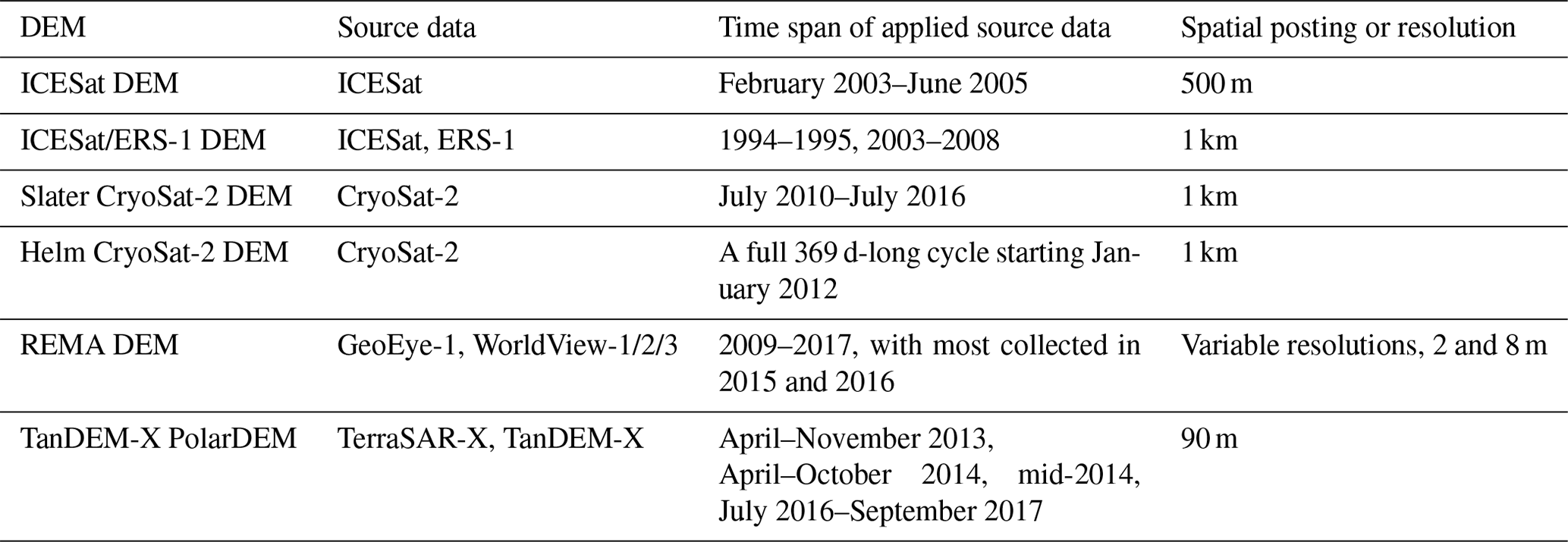
Due to the remoteness of Antarctica, most of the previously published Antarctic DEMs were derived from satellite or airborne data, e.g. elevation measurements from radar altimeters (Fricker et al., 2000; Helm et al., 2014; Slater et al., 2018), laser altimeters (DiMarzio et al., 2007), a combination of radar and laser altimeters (Bamber et al., 2009), stereophotogrammetry (Korona et al., 2009; Cook et al., 2012; Howat et al., 2019) and interferometry (Wessel et al., 2021). The currently available continent-scale Antarctic DEMs include one DEM derived from ICESat (hereafter called the ICESat DEM, DiMarzio et al., 2007), one based on the combination of ICESat and ERS-1 elevation measurements (hereafter called the ICESat/ERS-1 DEM, Bamber et al., 2009), two DEMs derived from CryoSat-2 (hereafter called the Helm CryoSat-2 DEM, Helm et al., 2014 and Slater CryoSat-2 DEM, Slater et al., 2018), one DEM derived from stereophotogrammetry using GeoEye-1 and WorldView-1/2/3 imageries (hereafter called the Reference Elevation Model of Antarctica, REMA, DEM, Howat et al., 2019), and one DEM derived from Interferometric Synthetic Aperture Radar (InSAR) using TerraSAR-X and TanDEM-X data (hereafter called the TanDEM-X PolarDEM, Wessel et al., 2021).
All these DEMs provide reasonable elevation estimates for Antarctica; however, some flaws still cannot be totally avoided. The coverage of ICESat is limited in ice sheet margins due to its coarse across-track resolution, hence for ICESat DEM most of the elevations in ice sheet margins were interpolated based on the neighbouring data. Although the ICESat/ERS-1 DEM improves the data coverage by combining the measurements from ICESat and ERS-1 elevations, this DEM aggregates observations spanning several years due to the different time spans (1994–1995 for ERS-1 and 2003–2008 for ICESat) of these two satellite altimeter datasets. This issue also exists with the REMA DEM and TanDEM-X PolarDEM, where multiyear satellite imageries were used. Different from the abovementioned DEMs, the Slater CryoSat-2 DEM was derived based on a model fitting method by using 7-year CryoSat-2 data (from July 2010 to July 2016). This method can quantify the measured elevation fluctuations due to interannual variations, and can provide a DEM for each month during the time span of applied data; however, although the radar penetration depth of the CryoSat-2 Ku-band into snowpack can be corrected either empirically or theoretically using a waveform fitting approach (Davis, 1996, 1997), the spatial and temporal variations of radar penetration depth are still difficult to account. As multitemporal and large-scale satellite radar altimeter data are usually used, the accuracy of estimated elevations is reduced. A similar problem also exists with the Helm CryoSat-2 DEM and TanDEM-X PolarDEM (the penetration depth of the X-band into snow may be several metres, Fischer et al., 2020; Dehecq et al., 2016).
The new generation satellite laser altimeter Ice, Cloud, And Land Elevation Satellite-2 (ICESat-2) of the National Aeronautics and Space Administration (NASA), which was launched on 15 September 2018, provides near-global (up to 88∘ S) and dense land ice elevation measurements in an accurate repeated cycle of 91 d by using a multibeam (6 beams in 3 pairs that work at 532 nm) laser altimeter (i.e. Advanced Topographic Laser Altimeter System, ATLAS, Neumann et al., 2019). The narrow footprint (approximately 17 m with a spatial interval of 0.7 m) and 3 pairs of beams (2 beams in 1 pair can determine the local slope) enable a fine-scale measurement of Antarctic surface heights even in steep regions. Hence, ICESat-2 can be expected to provide a new Antarctic DEM on a fine scale.
Here, we use a 1-year time series (from November 2018 to November 2019) of ICESat-2 elevation measurements to generate a new Antarctic DEM that covers both the ice sheet and ice shelves (hereafter called the ICESat-2 DEM). The applied data, DEM generation method and quality control criteria are presented in Sect. 2. Furthermore, we present the map of the ICESat-2 DEM and construct an accuracy evaluation by comparing it to the elevation measurements from the NASA Operation IceBridge (OIB) airborne mission and kinematic GPS and the Russian Global Navigation Satellite System (GLONASS) (GNSS) transects in Sect. 3. The performances of the ICESat-2 DEM and six currently available Antarctic DEMs are compared in Sect. 4, Sect. 5 provides the data availability and Sect. 6 summarizes the conclusions of this study.
2.1 ICESat-2 data
The ICESat-2 ATL06 land ice elevation product (version 3, Smith et al., 2019) from November 2018 to November 2019 is used. This product provides land ice elevation measurements at a spatial resolution of 20 m after correcting instrument-specific biases (i.e. corrections for transmit-pulse shape and first-photon bias, Neumann et al., 2019); here, only ATL06 data with good quality (according to the surface signal confidence metric from ATL06 data, i.e. those for which atl06_quality_summary equals zero) are used to generate the DEM. For the data collected over Antarctic ice shelves, corrections for ocean tide and inverse barometer effects are also applied (Egbert et al., 1994; Egbert and Erofeeva, 2002; Padman et al., 2002). Elevation measurements from all six beams are used to produce the densest surface height coverage. Although the signal energies of strong and weak beams are different, all six beams provide centimetre-scale elevation measurements, and the biases of two beams in one pair are less than 2 cm for flat regions (Brunt et al., 2019) and 5 cm for steep surfaces (Shen et al., 2021b). Thus, the effect of elevations estimated from weak beams is negligible.
2.2 NASA OIB airborne data and kinematic GNSS data
Elevation measurements from the OIB airborne mission in Antarctica are used here to evaluate the accuracy of the ICESat-2 DEM on a continental scale, including in the stable ice sheet interior and active marginal ice shelves. Surface heights from OIB airborne missions are measured by the Airborne Topographic Mapper (ATM), a conically scanning laser altimeter (at 532 nm) with a swath width of 140 m and footprint size of 1–3 m. The elevation measurement accuracy of the ATM is approximately 10 cm or better (Kurtz et al., 2013). Here, the IceBridge ATM L2 Icessn elevation, slope and roughness (V002) product (Studinger, 2014) is used, and a data filter (Young et al., 2008; Kwok et al., 2012; Studinger, 2014) is applied to remove abnormal values due to geolocation errors or cloud cover. To reduce the effect of interannual changes of surface elevations on DEM evaluation, the time difference between applied OIB airborne data and ICESat-2 DEM should be less than 1 year. Thus, OIB airborne data in October and November 2018 and October and November 2019 in Antarctica (Fig. 1) are chosen to evaluate the accuracy of the ICESat-2 DEM. In order to provide a comprehensive and more robust evaluation of the ICESat-2 DEM, OIB data in areas of low elevation change (i.e. ice sheet interior) from 2009 to 2017 are also used additionally (Fig. 1). The CryoSay-2 low rate mode (LRM) mask in Antarctica (which was designed for flat ice sheet interior measurements) is used to extract the regions of low elevation change. The CryoSat Geographical Mode Mask (V4.0, updated in 19–26 August 2019) at https://earth.esa.int/eogateway/news/cryosat-geographical-mode-mask-4-0-released (last access: 27 June 2022) is used. The averaged elevation change rate in the OIB data locations used is −0.0074 ± 0.0821 m yr−1 from 2003 to 2019, according to elevation change rate estimates from Smith et al. (2020). Hence, we assume that in these areas the effect of the elevation change on the DEM evaluation can be ignored. Besides, common OIB data in these areas from 2009 to 2019 (Fig. 1) are used to provide a robust and reasonable comparison between ICESat-2 DEM and previously published DEMs (see Sect. 2.3).
In addition, elevation records from kinematic GNSS observations (Schröder et al., 2017) in areas of low elevation change are also used for an additional DEM elevation comparison (Fig. 1). These GNSS profiles were measured in the region from the Vostok Station (106.8∘ E, 78.5∘ S) to the East Antarctic coast from 2001 to 2015 and an averaged offset of 4.9 cm was found compared to OIB airborne data in November 2013. A detailed introduction to the data collection, data processing method and accuracy evaluation can be found in Schröder et al. (2017).
Although OIB and GNSS data in the low elevation change areas and OIB data with a small time difference (< 1 year) compared to ICESat-2 DEM are used for DEM evaluation, the effect of the time difference between the DEM and evaluation data still needs to be considered. Here, we adjust the changes of ICESat-2 DEM elevation values which occur during the time difference between these two sets of data, the trend values are derived from Smith et al. (2020) and we assume the constant elevation change rates, the corresponding adjustments are calculated and applied for the DEM values in the locations of OIB and GNSS measurements before comparisons.

Figure 1Maps of the OIB airborne data in October and November 2018 and October and November 2019 (red), from 2009 to 2019 in ice sheet interior (blue). Map of the GNSS transects from 2001 to 2015 in Antarctica (yellow). The dashed lines show the boundary of the region where we assume there is low elevation change, which is the mode mask boundary of CryoSat-2 LRM data in Antarctica.
Table 1Detailed introduction to six previously published Antarctic DEMs, including the source data, time span of the source data, spatial posting or resolution.
2.3 Previously published Antarctic DEMs
The six previously published Antarctic DEM products are compared to the ICESat-2 DEM, i.e. ICESat DEM (DiMarzio et al., 2007), ICESat/ERS-1 DEM (Bamber et al., 2009), Helm CryoSat-2 DEM (Helm et al., 2014), Slater CryoSat-2 DEM (Slater et al., 2018), REMA DEM (Howat et al., 2019) and TanDEM-X PolarDEM (Wessel et al., 2021), as shown in Sect. 4. Detailed information concerning these DEMs is provided in Table 1, and all DEMs have been referenced to the WGS84 ellipsoid.
2.4 ICESat-2 DEM generation method
2.4.1 Surface elevation and uncertainty estimation
To separate the various contributions (i.e. local surface terrain and elevation change), following Slater et al. (2018) a model fitting method is applied here. The elevation is estimated using a quadratic function based on the local surface terrain and a time term (Eq. 1). This function is fitted in each grid (at resolutions of 500 m and 1 km, see following subsection) by using an iterative least-squares fit to all the included elevation measurements. By considering the surface elevation fluctuations and sub-annual changes, this method tends to obtain more accurate elevation estimates (Flament and Rémy, 2012; McMillan et al., 2014).
where E is the surface elevation derived from ICESat-2 measurement points, x and y are the local surface terrain respectively (i.e. the geographical locations), t is the time term, and is the DEM value in May 2019.
This method suits the ICESat-2 orbit cycle, which samples dense ground tracks comparing to previous satellite altimeters, more measurement points are included in the grid cell and the estimated elevations are more robust. It is possible for a quadratic form to model the topography at the resolutions of 500 m and 1 km and smaller elevation residuals can be found than using a simple linear fit (Flament and Remy, 2012). In addition, the model fitting method can provide the estimation of elevation change rate (a5), and the estimate agrees well with accurate elevation change estimations from the crossover points method (Moholdt et al., 2010), which provides an addition reference for the research of ice dynamics and mass balance.
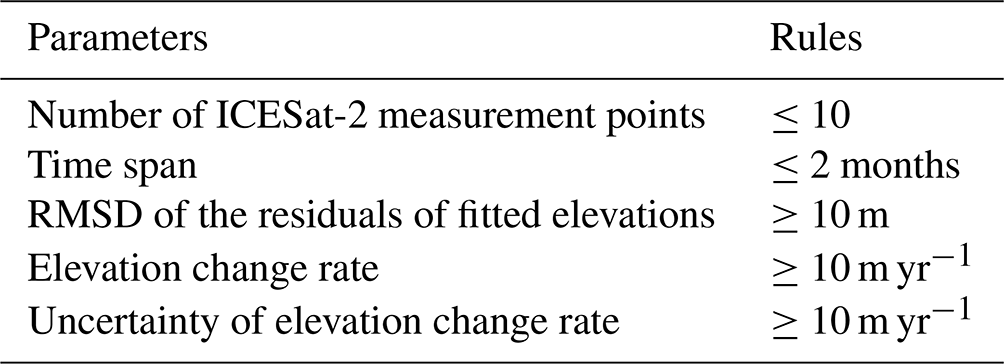
To reduce the effect of any poor fit the quality control criteria listed in Table 2 are performed, which includes the number of ICESat-2 measurement points used, the time span of the data used, the root-mean-square deviation (RMSD) of the residuals of fitted elevations, the elevation rate of change and the uncertainty. These criteria are constructed for all grid cells, and thus, there are some elevation gaps in the initial DEM. The remaining gaps are filled by using ordinary kriging interpolation (semi-variogram model: spherical, nugget: 0, sill: 1 652 285.953, radius: 10 km), which is widely used for generating previous DEMs (Helm et al., 2014; Slater et al., 2018). During the interpolation process, a search radius of 10 km is applied to obtain neighbouring measurement points. Similar estimation models have also been used in previous studies (Moholdt et al., 2010; Flament and Remy, 2012; McMillan et al., 2014; Konrad et al., 2017; Slater et al., 2018), and the evaluation in Sect. 3.2 also demonstrates its validity.
Table 2Quality control criteria applied to remove the unrealistic elevations due to the poor fitting performances in each grid cell.
The performance of this surface fit method is also affected by the spatial distribution and number of ICESat-2 measurement points. After quality control, 4.69 × 10⁹ ICESat-2 measurement points from November 2018 to November 2019 that cover all of Antarctica are used. An adequate number of ICESat-2 measurement points in one grid cell is required to generate valid elevation estimates. Figure 2 shows the distribution of the numbers of ICESat-2 measurement points used in individual grid cells (at the resolution of 500 m), which indicates a latitude-dependent pattern. Each grid cell contains approximately 118 ICESat-2 measurement points on average. In the ice sheet interior, the large coverage of ICESat-2 measurement points provides a complete surface height observation. In the low latitude region, the numbers of ICESat-2 measurement points are relatively small, the proportion of observed grid cells is reduced, and the representativeness is also reduced. Additionally, the performance of the surface fit method also depends on the time span of the input data, i.e. it should be noted that whether 1 year of ICESat-2 data can be used to obtain a satisfied fitting performance. Here we find that the elevation change rate map based on 1-year ICESat-2 data (i.e. a5 in Eq. 1) has a similar pattern to that from Smith et al. (2020), which estimated the elevation change rate from 2003 to 2019 based on ICESat and ICESat-2 data, indicating that 1 year of data can also provide the reasonable elevation change rates and thus the surface fit method used here is reliable.
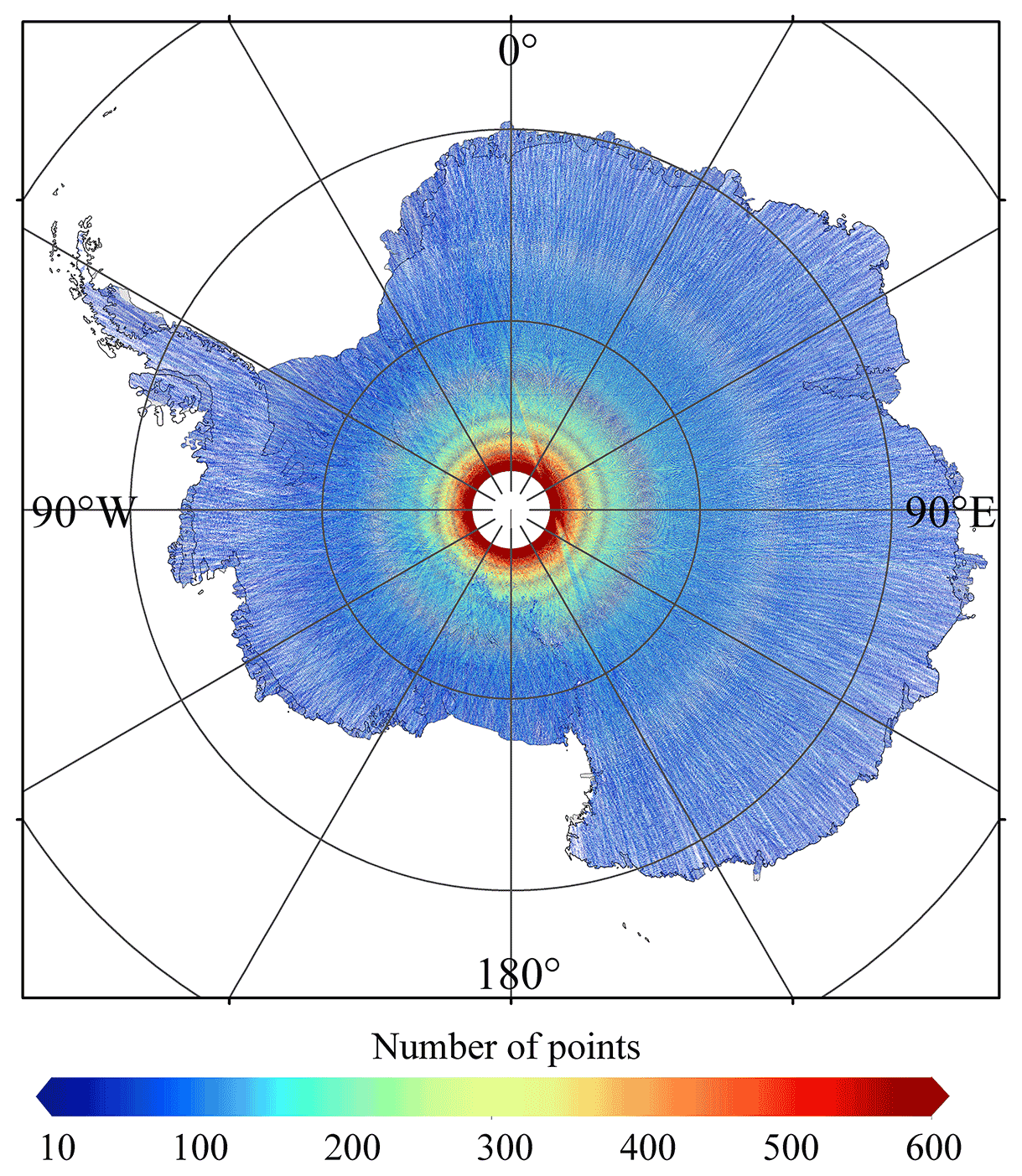
Figure 2Map of the numbers of valid ICESat-2 measurement points in each 500 m grid cell. The numbers of ICESat-2 measurement points in 1 km grid cells are resampled to the resolution of 500 m.
Uncertainties in DEM are calculated based on the approach described in Helm et al. (2014). The OIB elevation data are used as the reference and the elevation differences due to the time difference between OIB data and DEM are corrected based on the elevation change rates from Smith et al. (2020). The DEM uncertainty is then calculated from surface slope, roughness, number of data points used(N) and the elevation standard deviation (SD). Due to the difference in methods we calculate the DEM uncertainty for observed and interpolated grid cells. The surface slope and roughness are directly derived from the ICESat-2 DEM, the slope in one grid cell is derived as the maximum rate of change in elevation from that cell to its eight neighbours, the roughness is derived from the elevation difference between DEM and the smoothed DEM (by applying a 3 × 3 median filter). For observed grid cells, N is the number of data points in each grid cell used for elevation estimation; for interpolated grid cells, N is derived by counting all data points within the search radius of 10 km, which is the radius used for elevation interpolation and SD is the standard deviation of elevations of these data points. The differences between DEM and OIB elevations are calculated and firstly binned with reference to surface slope. The slope is divided into 200 bins with an interval of 0.01∘ (from 0 to 2∘), the median and standard deviation are calculated for each bin. This processing method is also applied for the other 3 parameters, an interval of 0.05 m for surface roughness, 250/500 (observed/interpolated grid cells) for N and 0.25 m for SD. For each distribution a 2-order polynomial is fitted by using the standard deviations of the elevation differences for each bin. The corresponding coefficients are listed in Table 3. This kind of polynomial order ensures a good and robust fitting performance, including for the small elevation differences in flat regions. Finally, the DEM uncertainty is calculated as follows:
where u is the DEM uncertainty, wi is the weighting factor, ui is the uncertainty for each uncertainty source, si is the scaling factor, σ is the standard deviation of the difference between the data and the polynomial fit and bi 0–3 are the coefficients for each polynomial fit (as listed in Table 3). When deriving the ICESat-2 DEM uncertainty estimation, the uncertainty from ICESat-2 measurements is not considered because the effect of ICESat-2 measurement bias is limited (< 5 cm, Brunt et al., 2019; < 14 cm, Shen et al., 2021b).
Table 3Fitting coefficients and weights used for the DEM uncertainty estimation.
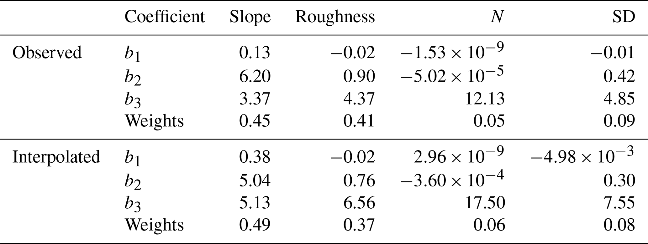
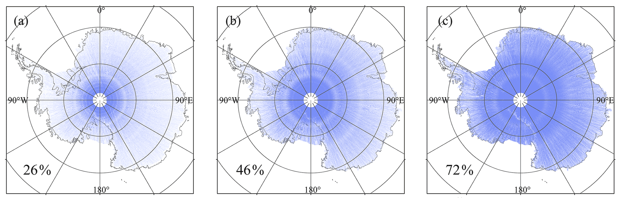
Figure 3Maps of the observed grid cells of DEMs at the spatial resolution of 250 m (a), 500 m (b) and 1 km (c). The observed grid cells are coloured in blue and the overall coverage of each DEM in Antarctica is also included.
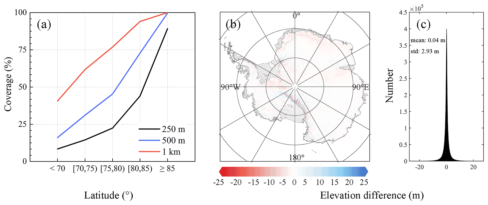
Figure 4(a) Spatial coverage of observed grid cells in the five latitude ranges when three spatial resolutions, i.e. 250 m (black), 500 m (blue) and 1 km (red), are applied. (b) Map of the elevation difference of DEMs at the resolutions of 1 km and 500 m. (c) Histograms of the elevation difference of DEMs at the resolutions of 1 km and 500 m, the average and standard deviation values are also included.
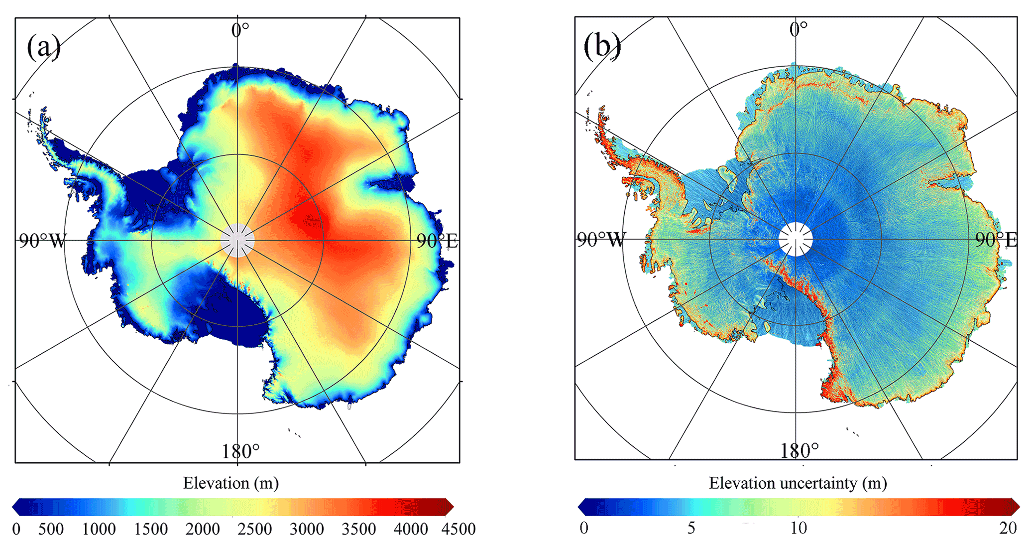
Figure 5(a) A new DEM of Antarctica at a posting of 500 m derived from ICESat-2, which covers both the ice sheet and ice shelves with the southern limit of 88∘ S. (b) Map of the ICESat-2 DEM elevation uncertainty.
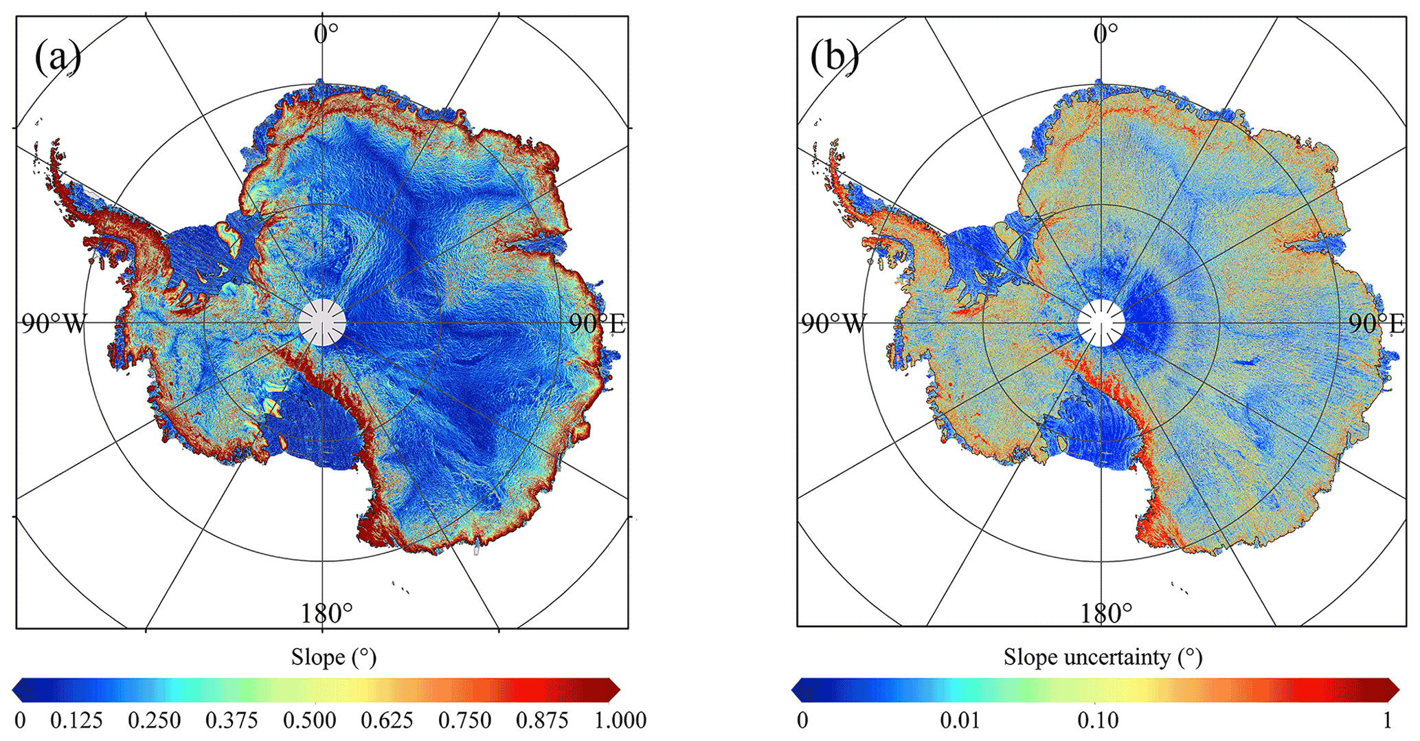
Figure 6(a) Map of the surface slope of Antarctica derived from the ICESat-2 DEM. (b) Map of the ICESat-2 DEM surface slope uncertainty. The uncertainty is estimated based on the propagation of elevation uncertainty.
2.4.2 Choice of DEM resolution
The selection criterion for DEM resolution is to present the detailed pattern of elevations and ensure enough spatial coverage of observed elevations (a smaller resolution tends to cause more observed elevation gaps). Although a much finer scale (e.g. 250 m) can reveal a more detailed elevation pattern, this contributes to more gaps among observed elevations. The overall spatial coverage of observed elevations when applying 250 m, 500 m and 1 km resolutions (which are usually applied in the Antarctic DEM) are 26 %, 46 % and 72 %, respectively. High latitude areas always have higher observed elevation coverages; in lower latitudes there are still some 250 m grid cells with estimated elevations (Fig. 3); however, 250 m DEM only has 26 % coverage. The detailed variations in the spatial coverages of observed grid cells at different latitudes at variable spatial resolutions (250 m, 500 m and 1 km, which are usually applied in the Antarctic DEM) are shown in Fig. 4a. A reliable grid size is 500 m, which provides denser spatial coverage of the observed elevations but a single resolution cannot obtain ideal spatial coverage, especially in low latitude areas. To increase the coverages of observed elevations as much as possible, referring to Slater et al. (2018), two spatial resolutions are used to estimate the surface elevations from ICESat-2, i.e. elevations are estimated at resolutions of 500 m and 1 km. The observation gaps in the 500 m DEM are filled by the resampled 1 km DEMs (resampled to the 500 m DEM). The addition of DEMs at 1 km greatly increases the observation coverage, the overall spatial coverage is approximately 74 %, and the remaining gaps are filled using ordinary kriging interpolation. Although two resolutions are applied, 1 km and interpolated elevations are both resampled to the posting of 500 m to provide a consistent DEM dataset; hence, the final ICESat-2 DEM is posted at a resolution of 500 m.
The application of two resolutions may include additional effects, i.e. different grid cell resolutions tend to present different elevation estimates. Here, we compare the elevation difference at the overlapped areas in Antarctica at different spatial resolutions (Fig. 4b). The elevation values become lower when a larger spatial resolution is applied, which acts as a running mean. Although applying different spatial resolutions affects the elevation values, an averaged elevation difference of 0.04 ± 2.93 m can be found (Fig. 4c), which is relatively small compared to the estimated elevations. In addition, this method can increase the coverage of observed elevations, and observed elevations tend to be more reliable than interpolated elevations (as shown in Sect. 3.2).
Finally, in order to remove additional elevation outliers in the generated DEM, a 3 standard deviation filter (3 × 3) is firstly applied. Visual inspection indicates that only a small number of anomalous elevations remain and these are further removed by using a 3 × 3 median filter. These quality assurance filters ensure the elevation pattern of the final DEM is smoothed and reasonable.
2.4.3 DEM evaluation method
The ICESat-2 DEM and previously published DEMs are resampled to the OIB and GNSS data locations and the differences for evaluation are calculated to reduce the effect of resolution differences between various DEMs. Four indexes are used to evaluate the DEM performance, including median deviation (MeD), median absolute deviation (MeAD), standard deviation (SD) and RMSD. The corresponding calculation equations are listed as follows:
where δi is the bias of ICESat-2 DEM and OIB or GNSS elevation, MD is the mean deviation and n is the number of the matched grid cells.
3.1 General attributes of ICESat-2 DEM
The effective time stamp of the ICESat-2 DEM is May 2019, which is halfway between November 2018 and November 2019. The ICESat-2 DEM provides a complete surface elevation reference for Antarctica, which illustrates higher elevations in the ice sheet interior and lower values in marginal ice shelves (Fig. 5). Negative elevations can be found in the ice shelves, especially in the Ross Ice Shelf. The local slope shows a pattern similar to the DEM, and undulated slopes are found in areas with rugged terrain, such as the Antarctic Peninsula and Transantarctic Mountains (Fig. 6). Both elevation and slope uncertainties show topography-dependent patterns, and larger values tend to be found at rugged areas, which may be related to the local surface conditions (i.e. slope and roughness). Larger elevation uncertainties can be found for interpolated grid cells than for observed ones, which is due to the difference in methods when deriving the surface elevations.
According to the shaded relief map of Antarctica derived from the ICESat-2 DEM (Fig. 7), obvious topographical patterns and flat terrain can be found in the mountain environments and ice sheet interior, respectively. On the Antarctic Peninsula, the ice shelf limit is visually identified from the shaded relief map (Fig. 7b). Other large-scale terrain features, e.g. subglacial lakes and floating ice shelves, can also be visually detected (Fig. 7c and d).
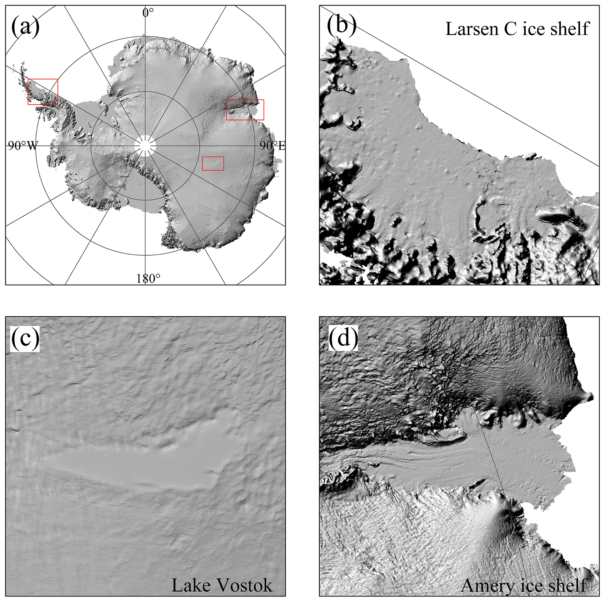
Figure 7(a) Shaded relief map of Antarctica derived from the ICESat-2 DEM. The detailed maps of the Larsen C ice shelf, Lake Vostok and Amery ice shelf are shown in (b), (c) and (d), respectively, and their locations are also shown in (a) by red rectangular boxes.
Two spatial resolutions are used in the ICESat-2 DEM, and the distributions of three kinds of grid cells (interpolated and observed at resolutions of 500 m and 1 km) show obvious latitude-dependent patterns. Regardless of whether at the basin scale or regional scale, more elevations at higher resolutions tend to be located in high-altitude areas, while elevations at lower or interpolated resolutions are mostly located in low-altitude regions (Fig. 8).
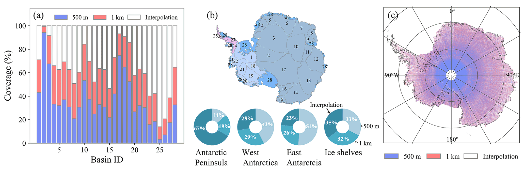
Figure 8(a) Coverage of observed grid cells at 500 m and 1 km and interpolated grid cells in 27 drainage basins of ice sheets (Zwally et al., 2012) and ice shelves. The boundaries and basin index (ID) of 27 ice sheet drainage basins (numbers 1–27) and ice shelves (number 28) are shown in (b). The coverages of observed (at two spatial resolutions) and interpolated grid cells in the Antarctic Peninsula, West Antarctica, East Antarctica and ice shelves are also shown in (b). Map of the selected grid cell resolution for deriving the ICESat-2 DEM in all grid cells at a spatial resolution of 500 m (c). Elevation values derived from 1 km and interpolation (i.e. 1 km) are resampled to a resolution of 500 m.
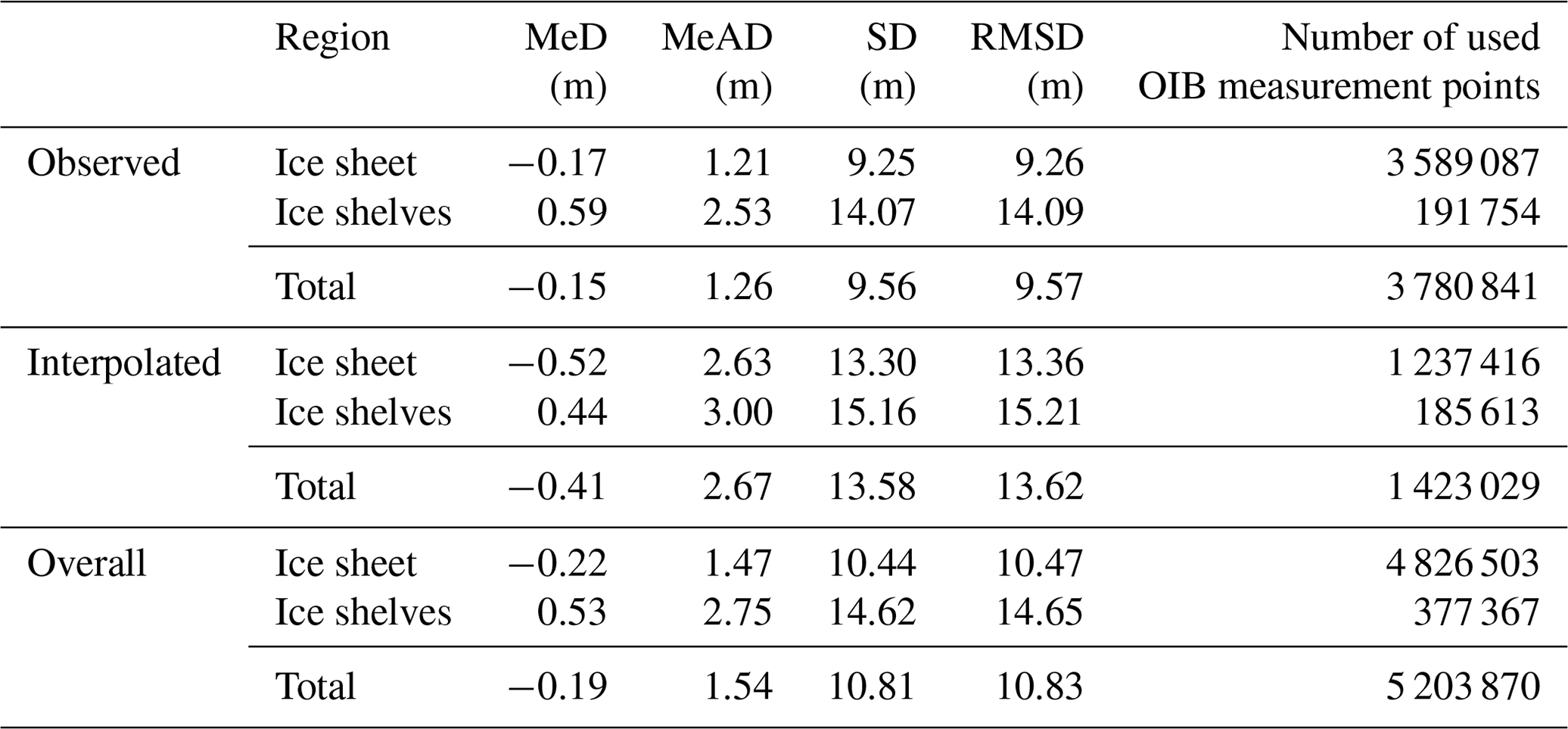
Table 4Comparisons between the ICESat-2 DEM and OIB airborne elevation measurements (including data in areas of low elevation change from 2009 to 2017 and data in the Antarctica from 2018 to 2019) in observed and interpolated areas for individual regions (i.e. the ice sheet and ice shelves). MeD: median deviation, MeAD: median absolute deviation, SD: standard deviation, RMSD: root-mean-square deviation.
3.2 Evaluation of ICESat-2 DEM by comparing to OIB airborne data
In total, approximately 5.2 × 10⁶ OIB measurement points that cover both the steep and flat regions (Fig. 1) are chosen to evaluate the ICESat-2 DEM. Generally, a MeAD of 1.54 m and an RMSD of 10.83 m are found for ICESat-2 DEM compared to OIB surface heights (Table 4). Ice sheet elevations are more accurate than those estimated for ice shelves, which may be due to a higher percentage of high-slope areas in ice shelves observed by OIB data than in ice sheets.
We also evaluate the elevation performance for observed and interpolated grid cells (Table 4). Generally, the bias of observed elevations is smaller than that of interpolated elevations in both ice sheets and ice shelves, which indicates that the observed elevations tend to be more accurate than those estimated from interpolation. Larger biases will be included in the ICESat-2 DEM if the coverage of interpolated elevations is high, hence the elevation gaps in the 500 m DEM are firstly filled by the resampled 1 km DEM to reduce the coverage of interpolated elevations. The accuracy of the ICESat-2 DEM has an obvious relationship with local terrain conditions, and the bias increases when the slope or roughness becomes larger, which is visible for three surface types (Table 5) and different surface slope conditions (Fig. 9). The bias in rocks is obviously larger than those for snow or firn and blue ice areas (BIAs), which is mainly due to the local terrain condition, as they are mostly located in the Transantarctic Mountains and the Antarctic Peninsula, while snow, firn and BIAs tend to have flat surface terrain; hence, they have a smaller bias. While in the low-slope regions, the ICESat-2 DEM shows good agreement with both the OIB and GNSS data, in the large-slope areas, larger biases occur (Fig. 9).
Table 5Comparison between the ICESat-2 DEM and OIB airborne elevation measurements (including data in areas of low elevation change from 2009 to 2017 and data in the Antarctica from 2018 to 2019) with respect to three surface types, i.e. snow or firn, blue ice areas (BIAs) and rocks. The surface type data are obtained from Hui et al. (2017).
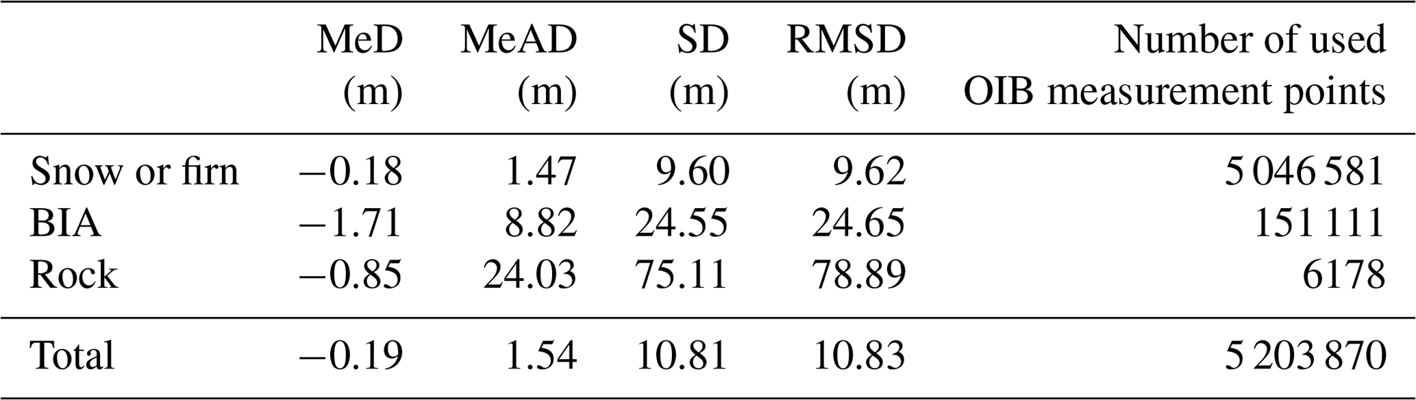
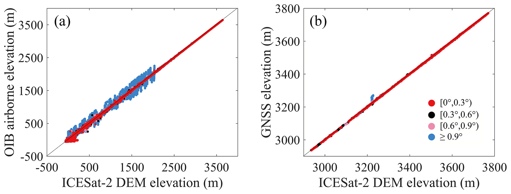
Figure 9Scatter plots of ICESat-2 DEM elevation and OIB airborne elevation (a) and GNSS elevation (b). The surface slopes are distinguished in different colours, as shown in the figure legend.
Although OIB airborne data provide an independent evaluation of the generated DEM, they still cannot present a comprehensive comparison. Most of the OIB airborne data were obtained in ice sheet margins or mountain environments, with high slopes and low elevations. Approximately 78 % of the OIB elevations used were less than 1500 m, and 76 % of the observed surface slopes from the OIB mission were less than 1∘, while the corresponding percentages from the ICESat-2 DEM are 36 % and 91 %, respectively. The OIB airborne data applied cannot completely represent the slope and elevation distributions of the Antarctic DEM; hence, the real accuracy of the ICESat-2 DEM is biased and may be higher.
In order to evaluate the DEM performance in more detail, the elevations along two OIB tracks in the flat ice sheet interior and rough ice sheet margins are shown in Fig. 10. In the ice sheet interior where surface slopes are small (Fig. 10a), elevation differences of approximately 5 m can be found (the median elevation difference for ICESat-2 DEM is −0.13 ± 0.19 m). The elevation differences are further reduced when the surface slopes become smaller. While at the Pine Island Glacier where surface slopes are large (Fig. 10b), elevation differences of approximately 20 m can be found in the undulating terrains (the median elevation difference is −0.01 ± 4.58 m). Overall, ICESat-2 DEM has better performances in the flat regions than steep areas. Regions of low surface slope represent the majority of Antarctic ice sheet, hence most elevations from ICESat-2 DEM have smaller elevation biases.
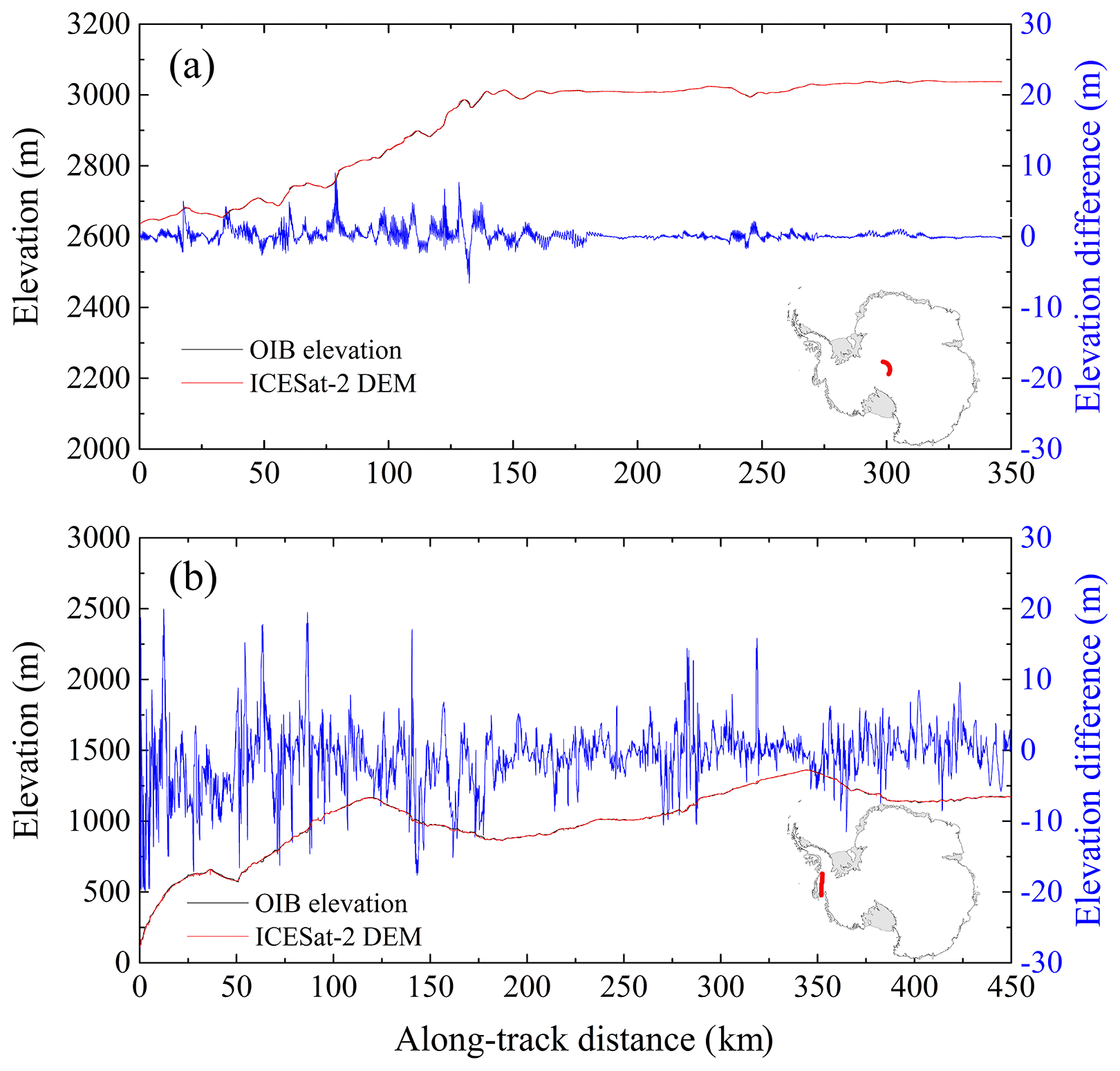
Figure 10Differences between the ICESat-2 DEM and OIB elevations along two OIB flight paths in (a) ice sheet interior and (b) Pine Island Glacier. ICESat-2 DEM elevations are in red, OIB elevations are in black, and the elevation differences between ICESat-2 DEM and OIB elevations are in blue. Locations of the two OIB flight paths are shown in red in the inserted figures of Antarctica.

Figure 11Elevation differences between the ICESat-2 DEM and six previously published DEMs, i.e. ICESat DEM (a), ICESat/ERS-1 DEM (b), Helm CryoSat-2 DEM (c), Slater CryoSat-2 DEM (d), REMA DEM (e) and TanDEM PolarDEM (f).
Additionally, by comparing to the OIB or GNSS elevation data (see Sect. 4), we can estimate the actual ICESat-2 DEM uncertainty as the SD of the differences to OIB or GNSS elevation data. In the estimated uncertainty map (Fig. 5b), a median value of 5.84 ± 5.29 m can be found. The SD of differences to OIB data shows a value of 10.44 m (Table 4, including plenty of measurements in ice sheet margins), while in the ice sheet interior a value of 3.26 m is found (Table 6). Considering the data coverage and surface slope difference, the estimated uncertainty values can represent the SDs from what is given as OIB, which means that the provided uncertainty estimates are reliable. A small SD value of 1.59 m can be found when comparing to the GNSS data (Table 7), which were obtained in the regions of low slope and may be due to the resolution and measurement accuracy differences between airborne and GNSS data; hence the ICESat-2 DEM uncertainty map may be slightly overestimated and can be assumed as the upper limit.
Table 6Comparisons between the ICESat-2 DEM, ICESat DEM, ICESat/ERS-1 DEM, Helm CryoSat-2 DEM, Slater CryoSat-2 DEM, REMA DEM, TanDEM PolarDEM and OIB airborne elevation measurements in areas of low elevation change from 2009 to 2019.
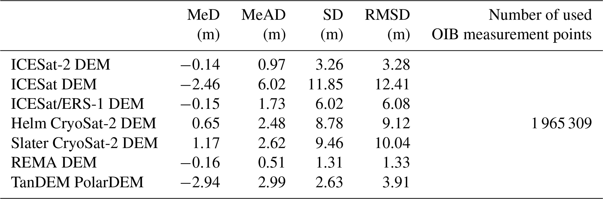

Figure 12Median differences between seven DEMs and OIB airborne elevation measurements in areas of low elevation change from 2009 to 2019 with respect to surface slope (a) and roughness (b). The upper and lower lines in each box indicate the 25th and 75th percentiles, the whiskers indicate the 5th and 95th percentiles, and the central horizontal line indicates the median difference.
When compared to the altimeter-derived DEMs, the elevation difference rises when the surface slope becomes larger, especially in mountainous environments (e.g. Transantarctic Mountains and Antarctic Peninsula, Fig. 11). This may be due to their differences in spatial resolution and measurement accuracy; this effect is considerably reduced when the local terrain is flatter (e.g. ice sheet interior). Compared to the REMA DEM and TanDEM PolarDEM, smaller elevation differences can be found in both the flat ice sheet interior and steep mountains and marginal ice sheets. REMA DEM and TanDEM PolarDEM have much smaller spatial resolutions and better performances and similar elevations indicate the reliability of ICESat-2 DEM in mountain environments. In particular, the ICESat-2 DEM shows a generally higher surface height than the TanDEM PolarDEM, which is assumed to be caused by the penetration depth of the X-band (TerraSAR-X and TanDEM-X) into snowpack (Dehecq et al., 2016; Fischer et al., 2020). Here it should be noted that the time differences between these DEMs can still cause the uncertainties in the DEM comparison.
To indicate a general comparison between the ICESat-2 DEM and other DEMs, OIB airborne data in areas of low elevation change from 2009 to 2019 are used to evaluate individual DEMs and the same evaluation method applied for the ICESat-2 DEM is used (as described in Sect. 2.2). The evaluation result shows that the ICESat-2 DEM has a reliable performance and is comparable to other DEMs derived from altimetry, stereo-photogrammetry and interferometry (Table 6).
The median differences in surface slope and roughness for these seven DEMs illustrate that all the elevation biases become more uncertain with increasing slope and roughness (Fig. 12). The REMA DEM always has more stable performances than the ICESat-2 DEM, as stereo-photogrammetry can generate more consistent elevation estimations at the regional scale than altimetry. A similar situation occurs for the TanDEM PolarDEM when slopes are > 1.5∘. Nevertheless, the ICESat-2 DEM is comparable to both the REMA DEM and TanDEM PolarDEM when slopes are less than 1∘, which occupies 91 % of Antarctica north of 88∘ S.
Here, kinematic GNSS data from 2001 to 2015 in the ice sheet interior are used to construct an additional DEM comparison. The comparison method and adjustment for time difference are the same as for OIB data. As surfaces in the interior of East Antarctica are flat, better performances for all DEM except TanDEM PolarDEM are found than those based on OIB airborne data. Similarly, ICESat-2 DEM has a reliable performance and is comparable to other DEMs (Table 7). Additionally, the accuracy of the ICESat-2 DEM may be related to the surface slope (Fig. 9b); however, as the terrain conditions of GNSS measurement points are relatively flat, this relationship is not obvious. It should be noted that the spatiotemporal coverages of the OIB and GNSS data used are limited here and they cannot provide an unbiased evaluation for ICESat-2 DEM and other DEMs. Hence the comparisons above only give a general reference for the performances and cannot be used as the quantitative accuracy evaluation.
Table 7Comparisons between the ICESat-2 DEM, ICESat DEM, ICESat/ERS-1 DEM, Helm CryoSat-2 DEM, Slater CryoSat-2 DEM, REMA DEM, TanDEM PolarDEM and GNSS elevation data in areas of low elevation change from 2001 to 2015.

Compared to other DEMs, the elevation change rate can be obtained when deriving the ICESat-2 DEM, which provides an additional reference for ice topography and mass balance estimation. Additionally, in previous studies several years of altimeter data are needed to derive the DEM in Antarctica. Due to the high-density measurements of ICESat-2, 13 months of ICESat-2 data can be used to generate a DEM for Antarctica and the performance is comparable to other DEMs, indicating that the ICESat-2 DEM can be updated annually. This study demonstrates the feasibility and reliability of using 1-year ICESat-2 data to derive the Antarctic DEM and provides a reference for the processing scheme of DEM (e.g. in higher resolution, regularly updated) based on ICESat-2 in future.
The generated ICESat-2 DEM (including the map of uncertainty) can be downloaded from the National Tibetan Plateau Data Center, Institute of Tibetan Plateau Research, Chinese Academy of Sciences at https://data.tpdc.ac.cn/en/disallow/9427069c-117e-4ff8-96e0-4b18eb7782cb/ (last access: 27 June 2022) (Shen et al., 2021a, https://doi.org/10.11888/Geogra.tpdc.271448).
A new DEM for Antarctica with a posting of 500 m is presented based on the surface height measurements from ICESat-2 by using a model fitting method. This DEM has an elevation measurement that accounts for 74 % of Antarctica, and the remaining 26 % is estimated based on the ordinary kriging method. The accuracy of the ICESat-2 DEM is evaluated by comparing it to the independent airborne data from the OIB mission. Overall, the ICESat-2 DEM shows a median bias of −0.19 m and an RMSD of 10.83 m, and these accuracies are compromises for DEM values from surface fits and interpolation. A median bias of −0.15 m and an RMSD of 9.57 m are found for areas where elevations are derived from ICESat-2 measurements, and they increase to −0.41 and 13.62 m, respectively, for interpolated elevations. The accuracy decreases when the surface slope or roughness increases; thus, larger biases occur for steep rocks, and flat snow or firn and blue ice areas have smaller elevation differences.
Compared to DEMs derived from satellite altimeters (i.e. the ICESat DEM, ICESat/ERS-1 DEM, Helm CryoSat-2 DEM, and Slater CryoSat-2 DEM), larger differences are found in regions with high slopes, which is due to their resolution difference, while smaller elevation differences compared to the REMA DEM and TanDEM PolarDEM support the reliability of the ICESat-2 DEM. Based on the OIB airborne data and kinematic GNSS transects, the ICESat-2 DEM shows reliable performance and is comparable to other DEMs, which further demonstrates the reliability of the ICESat-2 DEM.
Here 13 months of ICESat-2 data are used to generate the Antarctic DEM and the evaluation results show that the corresponding DEM is reasonable and valid. This means that the ICESat-2 DEM can be provided in a sustainable way, i.e. this DEM can be updated annually and thus accumulated on an annual basis. Additionally, reasonable elevation change rates can also be obtained when deriving the DEM. The combination of the derived DEMs and elevation change rates can be further used for the references of fieldwork planning, ice motion tracking, numerical modelling of ice sheets and the mass balance estimation. More importantly, these data can be provided on an annual basis, which has a large application potential for Antarctic research especially under climate warming.
XS and YF developed the related algorithm, generated and evaluated the ICESat-2 DEM; LD constructed the comparison to previously published DEM products; CQK supervised this work.
The contact author has declared that neither they nor their co-authors have any competing interests.
Publisher's note: Copernicus Publications remains neutral with regard to jurisdictional claims in published maps and institutional affiliations.
We thank all the data providers for their data. We thank the editors and reviewers for their constructive comments which helped to improve this manuscript.
This research has been supported by the National Natural Science Foundation of China (grant nos. 41976212, 41830105) and the Natural Science Foundation of Jiangsu Province (grant no. BK20210193).
This paper was edited by Baptiste Vandecrux and reviewed by Veit Helm and two anonymous referees.
Bamber, J., Vaughan, D., and Joughin, I.: Widespread complex flow in the interior of the Antarctic ice sheet, Science, 287, 1248–1250, https://doi.org/10.1126/science.287.5456.1248, 2000.
Bamber, J. L., Gomez-Dans, J. L., and Griggs, J. A.: A new 1 km digital elevation model of the Antarctic derived from combined satellite radar and laser data – Part 1: Data and methods, The Cryosphere, 3, 101–111, https://doi.org/10.5194/tc-3-101-2009, 2009.
Brunt, K., Neumann, T., and Smith, B.: Assessment of ICESat-2 ice sheet surface heights, based on comparisons over the interior of the Antarctic ice sheet, Geophys. Res. Lett., 46, 13072–13078, https://doi.org/10.1029/2019GL084886, 2019.
Cook, A. J., Murray, T., Luckman, A., Vaughan, D. G., and Barrand, N. E.: A new 100-m Digital Elevation Model of the Antarctic Peninsula derived from ASTER Global DEM: methods and accuracy assessment, Earth Syst. Sci. Data, 4, 129–142, https://doi.org/10.5194/essd-4-129-2012, 2012.
Cornford, S. L., Martin, D. F., Payne, A. J., Ng, E. G., Le Brocq, A. M., Gladstone, R. M., Edwards, T. L., Shannon, S. R., Agosta, C., van den Broeke, M. R., Hellmer, H. H., Krinner, G., Ligtenberg, S. R. M., Timmermann, R., and Vaughan, D. G.: Century-scale simulations of the response of the West Antarctic Ice Sheet to a warming climate, The Cryosphere, 9, 1579–1600, https://doi.org/10.5194/tc-9-1579-2015, 2015.
Davis, C. H.: Temporal change in the extinction coefficient of snow on the Greenland ice sheet from an analysis of Seasat and Geosat altimeter data, IEEE T. Geosci. Remote, 34, 1066–1073, https://doi.org/10.1109/36.536522, 1996.
Davis, C. H.: A robust threshold retracking algorithm for measuring ice-sheet surface elevation change from satellite radar altimeters, IEEE T. Geosci. Remote, 35, 974–979, https://doi.org/10.1109/36.602540, 1997.
Dehecq, A., Millan, R., Berthier, E., Gourmelen, N., Trouvé, E., and Vionnet, V.: Elevation changes inferred from TanDEM-X data over the Mont-Blanc area: Impact of the X-band interferometric bias, IEEE J. Sel. Top. Appl., 9, 3870–3882, https://doi.org/10.1109/JSTARS.2016.2581482, 2016.
DiMarzio, J., Brenner, A., Schutz, R., Shuman, C. A., and Zwally, H. J.: GLAS/ICESat 500 m laser altimetry digital elevation model of Antarctica., Boulder, Colorado USA, National Snow and Ice Data Center [data set], Digital media, https://doi.org/10.5067/K2IMI0L24BRJ, 2007.
Egbert, G. D. and Erofeeva, S. Y.: Efficient inverse modeling of barotropic ocean tides, J. Atmos. Ocean. Tech., 19, 183–204, https://doi.org/10.1175/1520-0426(2002)019<0183:EIMOBO>2.0.CO;2., 2002.
Egbert, G. D., Bennett, A. F., and Foreman, M. G.: TOPEX/POSEIDON tides estimated using a global inverse model, J. Geophys. Res.-Oceans, 99, 24821–24852, https://doi.org/10.1029/94JC01894, 1994.
Fischer, G., Papathanassiou, K. P., and Hajnsek, I.: Modeling and Compensation of the Penetration Bias in InSAR DEMs of Ice Sheets at Different Frequencies, IEEE J. Sel. Top. Appl., 13, 2698–2707, https://doi.org/10.1109/JSTARS.2020.2992530, 2020.
Flament, T. and Rémy, F.: Dynamic thinning of Antarctic glaciers from along-track repeat radar altimetry, J. Glaciol., 58, 830–840, https://doi.org/10.3189/2012JoG11J118, 2012.
Fricker, H. A., Hyland, G., Coleman, R., and Young, N. W.: Digital elevation models for the Lambert Glacier–Amery Ice Shelf system, East Antarctica, from ERS-1 satellite radar altimetry, J. Glaciol., 46, 553–560, https://doi.org/10.3189/172756500781832639, 2000.
Helm, V., Humbert, A., and Miller, H.: Elevation and elevation change of Greenland and Antarctica derived from CryoSat-2, The Cryosphere, 8, 1539–1559, https://doi.org/10.5194/tc-8-1539-2014, 2014.
Howat, I. M., Porter, C., Smith, B. E., Noh, M.-J., and Morin, P.: The Reference Elevation Model of Antarctica, The Cryosphere, 13, 665–674, https://doi.org/10.5194/tc-13-665-2019, 2019.
Hui, F., Kang, J., Liu, Y., Cheng, X., Gong, P., Wang, F., Li, Z., Ye, Y., and Guo, Z.: AntarcticaLC2000: The new Antarctic land cover database for the year 2000, Sci. China Earth Sci., 60, 686–696, https://doi.org/10.1007/s11430-016-0029-2, 2017.
Konrad, H., Gilbert, L., Cornford, S. L., Payne, A., Hogg, A., Muir, A., and Shepherd, A.: Uneven onset and pace of ice-dynamical imbalance in the Amundsen Sea Embayment, West Antarctica, Geophys. Res. Lett., 44, 910–918, https://doi.org/10.1002/2016GL070733, 2017.
Korona, J., Berthier, E., Bernard, M., Rémy, F., and Thouvenot, E.: SPIRIT. SPOT 5 stereoscopic survey of polar ice: reference images and topographies during the fourth International Polar Year (2007–2009), ISPRS J. Photogramm. Remote Sens., 64, 204–212, https://doi.org/10.1016/j.isprsjprs.2008.10.005, 2009.
Kurtz, N. T., Farrell, S. L., Studinger, M., Galin, N., Harbeck, J. P., Lindsay, R., Onana, V. D., Panzer, B., and Sonntag, J. G.: Sea ice thickness, freeboard, and snow depth products from Operation IceBridge airborne data, The Cryosphere, 7, 1035–1056, https://doi.org/10.5194/tc-7-1035-2013, 2013.
Kwok, R., Cunningham, G. F., Manizade, S. S., and Krabill, W. B.: Arctic sea ice freeboard from IceBridge acquisitions in 2009: Estimates and comparisons with ICESat, J. Geophys. Res.-Oceans, 117, C02018, https://doi.org/10.1029/2011JC007654, 2012.
McMillan, M., Shepherd, A., Sundal, A., Briggs, K., Muir, A., Ridout, A., Hogg, A., and Wingham, D.: Increased ice losses from Antarctica detected by CryoSat-2, Geophys. Res. Lett., 41, 3899–3905, https://doi.org/10.1002/2014GL060111, 2014.
Mengel, M., Nauels, A., Rogelj, J., and Schleussner, C.-F.: Committed sea-level rise under the Paris Agreement and the legacy of delayed mitigation action, Nat. Commun., 9, 1–10, https://doi.org/10.1038/s41467-018-02985-8, 2018.
Moholdt, G., Nuth, C., Hagen, J. O., and Kohler, J.: Recent elevation changes of Svalbard glaciers derived from ICESat laser altimetry, Remote Sens. Environ., 114, 2756–2767, https://doi.org/10.1016/j.rse.2010.06.008, 2010.
Neumann, T. A., Martino, A. J., Markus, T., Bae, S., Bock, M. R., Brenner, A. C., Brunt, K. M., Cavanaugh, J., Fernandes, S. T., and Hancock, D. W.: The Ice, Cloud, and Land Elevation Satellite–2 Mission: A global geolocated photon product derived from the advanced topographic laser altimeter system, Remote Sens. Environ., 233, 111325, https://doi.org/10.1016/j.rse.2019.111325, 2019.
Padman, L., Fricker, H. A., Coleman, R., Howard, S., and Erofeeva, L.: A new tide model for the Antarctic ice shelves and seas, Ann. Glaciol., 34, 247–254, https://doi.org/10.3189/172756402781817752, 2002.
Ritz, C., Edwards, T. L., Durand, G., Payne, A. J., Peyaud, V., and Hindmarsh, R. C.: Potential sea-level rise from Antarctic ice-sheet instability constrained by observations, Nature, 528, 115–118, https://doi.org/10.1038/nature16147, 2015.
Schröder, L., Richter, A., Fedorov, D. V., Eberlein, L., Brovkov, E. V., Popov, S. V., Knöfel, C., Horwath, M., Dietrich, R., Matveev, A. Y., Scheinert, M., and Lukin, V. V.: Validation of satellite altimetry by kinematic GNSS in central East Antarctica, The Cryosphere, 11, 1111–1130, https://doi.org/10.5194/tc-11-1111-2017, 2017.
Shen, X., Ke, C.-Q., and Fan, Y.: A digital elevation model of Antarctica derived from ICESat-2 (May 2019), National Tibetan Plateau Data Center [data set], https://doi.org/10.11888/Geogra.tpdc.271448, 2021a.
Shen, X., Ke, C.-Q., Yu, X., Cai, Y., and Fan, Y.: Evaluation of Ice, Cloud, And Land Elevation Satellite-2 (ICESat-2) land ice surface heights using Airborne Topographic Mapper (ATM) data in Antarctica, Int. J. Remote Sens., 42, 2556–2573, https://doi.org/10.1080/01431161.2020.1856962, 2021b.
Slater, T., Shepherd, A., McMillan, M., Muir, A., Gilbert, L., Hogg, A. E., Konrad, H., and Parrinello, T.: A new digital elevation model of Antarctica derived from CryoSat-2 altimetry, The Cryosphere, 12, 1551–1562, https://doi.org/10.5194/tc-12-1551-2018, 2018.
Smith, B., Fricker, H. A., Holschuh, N., Gardner, A. S., Adusumilli, S., Brunt, K. M., Csatho, B., Harbeck, K., Huth, A., and Neumann, T.: Land ice height-retrieval algorithm for NASA's ICESat-2 photon-counting laser altimeter, Remote Sens. Environ., 233, 111352, https://doi.org/10.1016/j.rse.2019.111352, 2019.
Smith, B., Fricker, H. A., Gardner, A. S., Medley, B., Nilsson, J., Paolo, F. S., Holschuh, N., Adusumilli, S., Brunt, K., Csatho, B., Harbeck, K., Markus, T., Neumann, T., Siegfried, M. R., and Zwally, H. J.: Pervasive ice sheet mass loss reflects competing ocean and atmosphere processes, Science, 368, 1239–1242, https://doi.org/10.1126/science.aaz5845, 2020.
Studinger, M.: IceBridge ATM L2 Icessn Elevation, Slope, and Roughness, version 2. Boulder, Colorado USA, National Snow and Ice Data Center [data set], Digital media, https://doi.org/10.5067/CPRXXK3F39RV, 2014.
Wesche, C., Eisen, O., Oerter, H., Schulte, D., and Steinhage, D.: Surface topography and ice flow in the vicinity of the EDML deep-drilling site, Antarctica, J. Glaciol., 53, 442–448, https://doi.org/10.3189/002214307783258512, 2007.
Wessel, B., Huber, M., Wohlfart, C., Bertram, A., Osterkamp, N., Marschalk, U., Gruber, A., Reuß, F., Abdullahi, S., Georg, I., and Roth, A.: TanDEM-X PolarDEM 90 m of Antarctica: generation and error characterization, The Cryosphere, 15, 5241–5260, https://doi.org/10.5194/tc-15-5241-2021, 2021.
Young, D. A., Kempf, S. D., Blankenship, D. D., Holt, J. W., and Morse, D. L.: New airborne laser altimetry over the Thwaites Glacier catchment, West Antarctica, Geochem. Geophy. Geosy., 9, Q06006, https://doi.org/10.1029/2007GC001935, 2008.
Zwally, H. J., Giovinetto, M. B., Beckley, M. A., and Saba, J. L.: Antarctic and Greenland Drainage Systems, NASA's Goddard Space Flight Center: Cryospheric Sciences Laboratory, Digital media, https://earth.gsfc.nasa.gov/cryo/data/polar-altimetry/antarctic-and-greenland-drainage-system (last access: 27 June 2022), 2012.