Historical and future weather data for dynamic building simulations in Belgium using the regional climate model MAR: typical and extreme meteorological year and heatwaves

Increasing temperatures due to global warming will influence building, heating, and cooling practices. Therefore, this data set aims to provide formatted and adapted meteorological data for specific users who work in building design, architecture, building energy management systems, modelling renewable energy conversion systems, or others interested in this kind of projected weather data. These meteorological data are produced from the regional climate model MAR (Modèle Atmosphérique Régional in French) simulations. This regional model, adapted and validated over Belgium, is forced firstly, by the ERA5 reanalysis, which represents the closest climate to reality and secondly, by three Earth system models (ESMs) from the Sixth Coupled Model Intercomparison Project database, namely, BCC-CSM2-MR, MPI-ESM.1.2, and MIROC6. The main advantage of using the MAR model is that the generated weather data have a high resolution (hourly data and 5 km) and are spatially and temporally homogeneous. The generated weather data follow two protocols. On the one hand, the Typical Meteorological Year (TMY) and eXtreme Meteorological Year (XMY) files are generated largely inspired by the method proposed by the standard ISO15927-4, allowing the reconstruction of typical and extreme years, while keeping a plausible variability of the meteorological data. On the other hand, the heatwave event (HWE) meteorological data are generated according to a method used to detect the heatwave events and to classify them according to three criteria of the heatwave (the most intense, the longest duration, and the highest temperature). All generated weather data are freely available on the open online repository Zenodo (https://doi.org/10.5281/zenodo.5606983, Doutreloup and Fettweis, 2021) and these data are produced within the framework of the research project OCCuPANt (https://www.occupant.uliege.be/ (last access: 24 June 2022)​​​​​​​ – ULiège).

1 Introduction

On a global scale, the warmest (SSP5-8.5) scenario from the IPCC last assessment report (IPCC, 2021) suggests a temperature increase of +5 ^∘C by 2100. However, the regions of the world will not warm up at the same speed or intensity. Some regions, such as the poles, will warm faster and to higher levels than equatorial regions (Lee et al., 2021). Over the temperate regions, such as western Europe, the temperature is expected to increase between +1 and +5 ^∘C in 2100, depending on the climate models and greenhouse gas emission scenarios used (Termonia et al., 2018; RMI, 2020; IPCC, 2021).

Moreover, IPCC (2021) affirm that extreme events will become more probable and more intense. In particular, the maximum temperature is expected to increase faster (sometimes up to twice) than the mean temperature (Seneviratne et al., 2021). Over western-central Europe, maximum temperatures are projected to increase up to +7 ^∘C for a global increase of +5 ^∘C (Seneviratne et al., 2021).

More concretely, in the summer, hot extremes (including heatwaves) are already increasing and will continue to strengthen with global warming, both in intensity and frequency (Suarez-Gutierrez et al., 2020; Seneviratne et al., 2021; Dunn et al., 2020). The consequences of these heatwaves will affect human health (Fouillet et al., 2006), agriculture, the comfort and health of life inside buildings (Bruffaerts et al., 2018; Sherwood and Huber, 2010; Buysse et al., 2010), and the energy demand, especially for cooling systems (Larsen et al., 2020). This is what motivated some previous studies in Belgium to represent the energy needs for heating and cooling under average and extreme weather conditions (Ramon et al., 2019).

Energy efficiency and living comfort are precisely what motivates the ULiège OCCuPANt project (Impacts Of Climate Change on the indoor environmental and energy PerformAnce of buildiNgs in Belgium during summer, https://www.occupant.uliege.be/, last access: 24 June 2022), in which climate data are involved. The OCCuPANt project aims to evaluate the energy performance and vulnerability of building inhabitants in the context of climate change. Acquiring reliable current and future climate data is vital in any study related to climate change and defines its quality (Pérez-Andreu and al., 2018).

The purpose of this data set is to propose meteorological data coming from a fine-resolution regional climate model over Belgium and neighbouring regions. These data will then be used to anticipate future climate changes, which will influence both the production of heating and cooling demands as well as the electrical grids on larger scales. These changes will require innovations in building design and systems, which will necessarily take time. Thus, the more they are anticipated, the better we will find solutions. The use of a regional model allows the building of spatially and temporally continuous and homogeneous past and future meteorological data, according to different warming scenarios for some Belgian cities. This regional model is fed by the ERA-5 reanalysis model (Hersbach et al., 2020) to simulate the past climate (1980–2020), and also by three different Earth system models (ESMs) from the Sixth Coupled Model Intercomparison Project (CMIP6) database (Wu et al., 2019; Tatebe et al., 2019; Gutjahr et al., 2019) to obtain different future projections and associated uncertainties for the same scenario SSP5-8.5.

The future climate data are very useful to predict the variations in heating and cooling demands in buildings. The characterisation of a minimum outdoor temperature under future scenarios is necessary to estimate the heating and cooling season needs. This can result in rethinking building designs and making them resilient against the impact of climate change. For instance, in the heating-dominated region of Belgium, the concept of building design focuses more on heat retention to decrease heating energy use during the winter. However, warming weather conditions in the last decades meant that this design concept caused significant overheating problems during the summer. Therefore, it is necessary to predict the future performance of buildings and adapt them to the variations in outdoor weather conditions. Designing cooling systems that can last for 100 years is challenging. However, it is possible to increase the preparedness of buildings for climate change through passive design strategies, the use of active heating/cooling systems, or both. Both active and passive solutions may need regular replacements over the building's lifespan.

For each city, considered period, model, and scenario, two synthetic files (in CSV format) are generated, largely inspired by the method in ISO-15927-4. These are a Typical Meteorological Year (TMY) file and an eXtreme Meteorological Year (XMY) file. In addition to these synthetic files, files focused on heatwaves are also generated, namely, a file for the most intense heatwave event, one for the warmest heatwave, one for the longest heatwave, and one containing all the heatwaves detected within a specific period. These files are described in detail in the Methodology section.

2 Methodology

2.1 MAR model and area of interest

The regional climate model used in this study is the Modèle Atmosphérique Régional model (hereafter MAR) in its version 3.11.4 (Kittel, 2021). The main role of MAR is to downscale a global model or reanalysis to get weather outputs at a finer spatial and temporal resolution (Fig. 1). As shown in Fig. 1, MAR is a 3-dimensional atmospheric model coupled to a 1-dimensional transfer scheme between the surface, vegetation, and atmosphere (Ridder and Gallée, 1998). The MAR model also includes an urban island module, which modifies the city grid points to simulate an urban heat island through a modification of the surface albedo (fixed to 0.1) and an absence of vegetation, which influence the thermal and humidity exchanges between soil and atmosphere. Initially, the MAR model was developed for both Greenland (Fettweis et al., 2013) and Antarctica ice sheets (Agosta et al., 2019; Kittel et al., 2021). However, it has recently been successfully adapted to temperate regions such as Belgium (Fettweis et al., 2017; Doutreloup et al., 2019; Wyard et al., 2021). In the framework of this study, MAR is initially forced every 6 h at its lateral boundaries (temperature, wind, and specific humidity) by the reanalysis ERA5 (hereafter called MAR-ERA5), which is available at a horizontal resolution of ∼ 31 km (Hersbach et al., 2020). Different kinds of observations (in situ weather observations, radar data, satellites, etc.) are 6-hourly assimilated into ERA5 to be closest to the observed climate. In this way, the simulations of MAR-ERA5 can be considered as the closest simulation to the current observed climate.

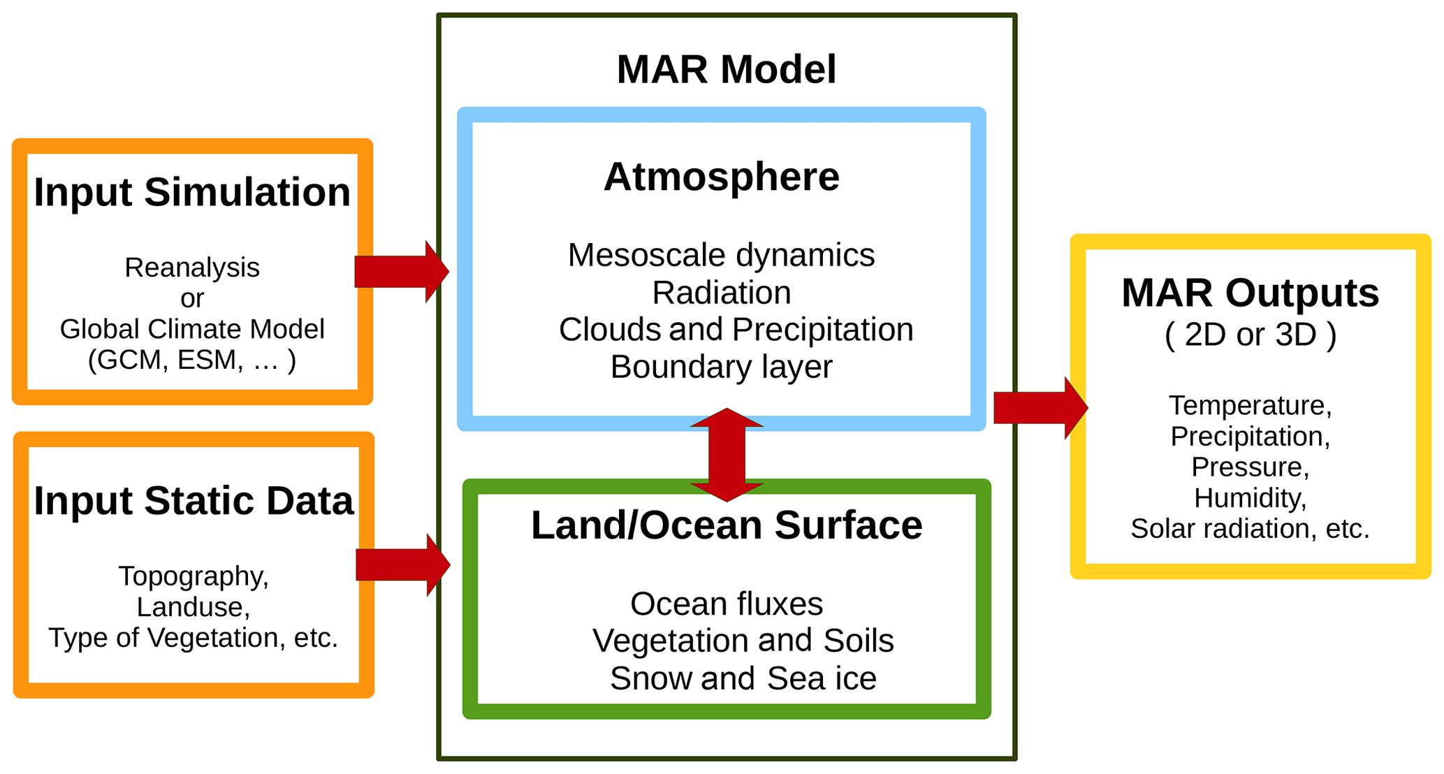
Figure 1 Workflow of the MAR model. The MAR model (black box) needs to be forced by a reanalysis model or global model (upper orange box) and by static data (lower orange box). The result of the MAR simulation gives meteorological variables in two or three dimensions (yellow box).

Then, the MAR model has been forced every 6 h by three ESMs from the CMIP6 database (Eyring et al., 2016). These ESMs do not contain any observational data and represent only an evolution of the average and interannual variability of the climatic parameters over long periods. These models contain two characteristic periods: one in the past from 1980 to 2014 (hereafter called the “historical” scenario) and another in the future from 2015 to 2100 according to different SSP scenarios (SSP5-8.5, SSP3-7.0, and SSP2-4.5). The selection and description of each of these ESMs and a comparison with MAR-ERA5 over the historical period are presented in the next section.

The atmospheric variables used to force MAR every 6 h at each vertical level are temperature, surface pressure, wind, specific humidity, and the sea surface temperature over the North Sea from both ERA5 reanalysis (from 1980 to 2020) and the three ESMs (from 1980 to 2100). The spatial resolution of MAR is 5 km over an integration domain (120 × 90 grid cells) centred over Belgium, as shown in Fig. 2, to build hourly outputs.

Figure 2 Model topography (colour background and dashed black line, both in metres above sea level), localisation of cities (black letters) used in this dataset for Belgium, and localisation of neighbouring countries (in red letters).

The choice of 12 cities is motivated, on the one hand, by the size of the cities which must be sufficient to show a temperature increase compared to the neighbouring countryside and, on the other hand, to best represent the climate spatial variability observed in Belgium. For example, the city of Oostende is strongly influenced by the thermal inertia of the sea, while the city of Arlon has a more continental climate.

2.2 Forcing models and MAR simulations

2.2.1 Choice of representative Earth system models

The Sixth Coupled Model Intercomparison Project (CMIP6; Eyring et al., 2016) database contains about 30 ESMs from many scientific institutes around the world. For practical reasons, we cannot regionalise all these ESMs. Thus, we had to select a few representative ESMs for our region of interest, western Europe.

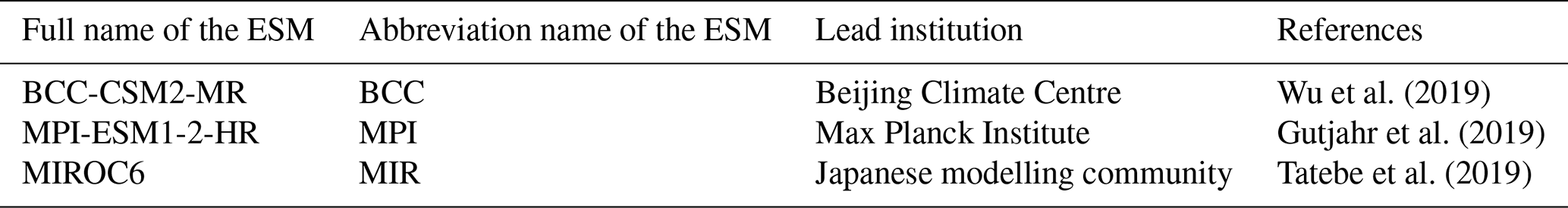
Our choice was based on two criteria. The first criterion is that the ESM should represent (with the lowest possible bias) the main atmospheric circulation in the free atmosphere over western Europe by evaluating the geopotential height at 500 hPa and the temperature at 700 hPa during summer and winter, with respect to ERA5 over 1980–2014 based on the skill score method developed by Connolley and Bracegirdle (2007). After selecting the ESMs that meet this first criterion, the second criterion is to choose three ESMs representing the CMIP6 models spread in 2100 for the same scenario (SSP5-8.5 here). Namely, we keep only three ESMs (see Table A1): BCC-CSM2-MR (Wu et al., 2019), MPI-ESM.1.2 (Gutjahr et al., 2019), and MIROC6 (Tatebe et al., 2019). The ESM BCC-CSM2-MR simulates warming close to the ensemble mean of the 30 ESMs for the 2100 horizon using the SSP5-8.5 scenario, the ESM MIROC6 simulates larger warming than the ensemble mean, and the ESM MPI-ESM.1.2 simulates lower warming than the ensemble mean by 2100. The use of these three models allows us to obtain a first approximation of the uncertainty from ESMs without having to downscale all 30 available models of CMIP6.

2.2.2 Future socio-economic scenarios

Shared Socio-economic Pathways (SSPs; Riahi et al., 2017) are scenarios of global socio-economic evolution projected to 2100. These SSPs are used to develop greenhouse gas (GHG) emission scenarios associated with different climate policies and are used to force each future ESM. There are three main scenarios, namely SSP2-4.5 (intermediate GHGs), SSP3-7.0 (high GHGs) and SSP5-8.5 (very high GHGs), causing global warming for 2100 to increase respectively. For more details about these scenarios, we refer to Riahi et al. (2017). Finally, it should be noted that the historical scenario mentioned in Sect. 2.1 is forced by the greenhouse gas concentrations observed over the period of 1980–2014.

For the same practical reasons that led us to choose only three ESMs out of the 30 available models, we cannot afford to calculate every SSP scenario of each ESM. However, as the ESMs cannot represent general circulation changes (Eyring et al., 2021), the use of one scenario or another will not cause more blocking anticyclones leading to more persistent heatwaves, for example. Thus, whichever scenario is used will only reflect temperature changes in relation to its GHG concentrations. Hence, only the SSP5-8.5 scenario has been calculated and the other scenarios (SSP3-7.0 and SSP2-4.5) are derived from the MAR simulations forced by the ESMs using the SSP5-8.5 scenario, since the warming rates from lower scenarios are included in the scenario SSP5-8.5, but for a different earlier time period. Thus, for each scenario (SSP3-7.0 and SSP2-4.5), the equivalent warming period in the SSP5-8.5 scenario has been found according to these three steps:

1. The raw 2 m annual mean temperature of each ESM and each scenario has been aggregated over Belgium to the horizon 2100.

2. For each ESM, the equivalent 20-year period from the SSP5-8.5 scenario has been chosen as the period with the closest mean and the closest interannual variability of the 2 m annual temperature, compared to the future 20-year period (i.e. 2021–2040, 2041–2060, …) from the two other scenarios (SSP3-7.5 and SSP2-4.5).

3. Once the equivalent warming period has been identified, the data of this period are extracted out of the SSP5-8.5-forced MAR simulations for both SSP3-7.5 and SSP2-4.5 scenarios.

For example, the data of MAR-MPI for SSP3-7.0 over 2081–2100 are the outputs of MAR-MPI using SSP5-8.5 over the period 2066–2085.

This method is open to discussion for several reasons. Firstly, the climate does not react in a linear way to an increase of GHG flowing through the different SSP scenarios. Moreover, with an equal warming rate, but different periods, the earth, atmosphere and ocean systems will not have the same (spatial and temporal) responses due to their inertia. Despite these precautions, this methodology allows us, on the one hand, to derive a quick estimation without additional computer time. On the other hand, it remains valid as a first approximation, especially since the most interesting weather variable in this study is temperature, which is, by construction, the least sensitive to these issues.

2.2.3 Evaluation of the MAR simulations

To verify that these ESM-forced MAR simulations can be used to anticipate future periods, it is necessary to evaluate them over the overlapping period between the ERA5 reanalyses and the historical scenario (namely, 1980–2014). The aim is to determine if they can represent the average and climate variability over the Belgian territory for this period as observed (i.e. ERA5 in our case). So, we compare the three MAR simulations forced by the three ESMs with the MAR simulation forced by the ERA5 reanalyses. As the most important variable for this database is the temperature at 2 m above ground level (a.g.l.) and an important secondary variable is the incoming solar radiation, the mean and standard deviation of these data over the period 1980–2014 and over the Belgian territory are compared in Table 1 and Fig. 3. These values are compared on an annual scale and on a summer scale since the OCCuPANt project focuses on heatwaves.

Table 1 Comparison of MAR-ERA5 (i.e. MAR forced by the reanalysis ERA5) with MAR-BCC (i.e. MAR forced by BCC-CSM2-MR), MAR-MPI (i.e. MAR forced by MPI-ESM.1.2), and MAR-MIR (i.e. MAR forced by MIROC6) to mean temperature at 2 m above ground level and mean incoming solar radiation over Belgium's territory during 1980–2014 (mean value ± standard error).

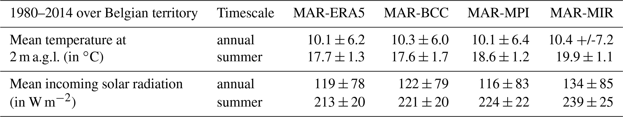
Figure 3 Annual mean temperature (in ^∘C​​​​​​​, lower lines) and annual summer temperature (in ^∘C, upper lines) of MAR forced by ERA5 reanalysis (in black lines between 1980 and 2020), MAR-BCC (i.e. MAR forced by BCC-CSM2-MR in red lines), MAR-MPI (i.e. MAR forced by MPI-ESM.1.2 in blue lines), and MAR-MIR (i.e. MAR forced by MIROC6 in green lines) between 1980 and 2100 according to the scenario SSP5-8.5. The average is computed here over the whole integration domain, excluding the ocean.

The results of this comparison presented in Table 1 indicate that the incoming solar radiations and temperature at 2 m a.g.l. values proposed by the three MAR simulations forced by the ESMs are mostly close to the average simulated by MAR-ERA5, with (not statistically significant) biases between MAR forced by the ESMs and MAR-ERA5 lower than the standard deviation (i.e. the interannual variability) of MAR-ERA5. We can also note that the interannual variability of the MAR simulations forced by the ESMs is close to the interannual variability of the MAR-ERA5 simulation. We can then conclude that the MAR simulations forced by the ESMs can represent the mean climate simulated by MAR-ERA5 and its interannual variability with success, except MAR-MIR, which significantly overestimates temperature and solar radiation in summer. Knowing that MAR-MIR simulated the largest warming in 2100, this simulation needs to be considered as the extreme climate we could have.

2.3 Generating the Typical Meteorological Year and eXtreme Meteorological Year files

The Typical Meteorological Year (TMY) and the eXtreme Meteorological Year (XMY) are data sets that are widely used by building designers and others to model renewable energy conversion systems (Wilcox and Marion, 2008). The TMYs are the synthetic years (on an hourly basis) constructed by representative typical months (Barnaby and Crawley, 2011), which are selected by comparing the distribution of each month within the long-term (minimum of 10 years) distribution of that month for the available observations or modelled data (using Finkelstein–Schafer statistics (Finkelstein and Schafer, 1971). The XMY is the extension of the TMY weather data and is formed by selecting the most deviating (i.e. extreme) months over a certain data set instead of typical months (Ferrari and Lee, 2008). There are many methods to reconstruct this kind of weather file (Ramon et al., 2019), but for this study, a protocol for the construction of these typical years has been developed based on the ISO15927-4 (European Standard, 2005) and is described briefly below.

The method consists of reconstituting each month of the typical (extreme) year with the most typical (extreme) month present in the considered period for a considered city. The comparison is essentially based on two variables, namely, temperature at 2 m a.g.l. and incoming solar radiation. The choice of these two climatic parameters is related to the fact that they both influence the comfort inside the buildings. Therefore, we generate files with the typical year according to the temperature at 2 m a.g.l. and a typical year according to the incoming solar radiation.

Here are the steps to find the most typical (extreme) month for each climatic parameter:

1. Converting an hourly file into a daily file: from all the hourly data from all the same calendar months available within the selected period, the daily mean of the climatic parameter is computed.

2. Selecting the typical (extreme) month: for each calendar month, the percentile 50 (95) of the climatic parameter is calculated over the studied period to find the month that is the closest to the 50 percentile (95) of this climatic parameter.

3. Extracting hourly data of this typical (extreme) month: finally, the hourly weather values of this typical (extreme) month are stored in the file of the typical (extreme) year.

The hourly weather variables available in the TMY and XMY files are described in Table 2.

Table 2 Name, level, and units of all weather variables used in the produced weather files.

2.4 Definition of a heatwave and generating heatwave event files

In Belgium, heatwaves are officially defined by two definitions: a retrospective one and a prospective one. The retrospective heatwave is defined as periods of at least five consecutive days with a maximum temperature higher than 25 ^∘C, of which, at least 3 days within this period has a maximum temperature higher than 30 ^∘C (RMI, 2020). The prospective heatwave is a period with a predicted minimum temperature of 18.2 ^∘C or more and a maximum temperature of 29.6 ^∘C or higher, both for three consecutive days (Brits et al., 2009).

However, these definitions are static and do not consider the local climate of each region. For example, in the highlands (with altitudes above 300 m in Fig. 2) where it is on average colder, these heatwave criteria are not necessarily met, even though this region also experiences a heatwave. Moreover, when comparing the different ESMs, this fixed heatwave definition criterion could induce artefacts, since each ESM has its own variability and biases over the current climate. For these reasons, we have used the statistical definition of a heatwave from Ouzeau et al. (2016), computed for each MAR pixel regardless of its basic climate and each ESM independently of its own internal variability.

The calculation method, according to Ouzeau et al. (2016), is as follows and it is illustrated in Fig. 4:

• For the period 1980–2014 (which corresponds to the “historical” scenario in the ESMs), for each pixel and each MAR simulation, we calculate three thresholds defined by three percentiles of the daily mean temperature: Sint = 95th​​​​​​​ percentile, Sdeb = 97.5th percentile, and Spic = 99.5th percentile.

• A heatwave is detected when the daily mean temperature reaches Spic. The duration of this event is the number of days between the first day when the daily mean temperature is equal to or greater than Sdeb, and either when the daily mean temperature falls below Sint or when the daily mean temperature falls below Sdeb for at least three consecutive days.

• In this data set, we add a condition compared to Ouzeau et al. (2016), which is that the minimum duration of the heatwave must be at least five consecutive days, otherwise the heatwave event is not considered as such.

Once the heatwave events (called HWE hereafter) are detected, we can characterise them according to three criteria:

1. the duration, which is the number of consecutive days of the HWE;

2. the maximal daily mean temperature reached during the HWE;

3. the global intensity, which is calculated by the cumulative difference between the temperature and the Sdeb threshold during the HWE, divided by the difference between Spic and Sdeb.

The hourly data provided in each HWE file are the same as for the TMY and XMY files (see section above). For each period, each city, each scenario, and each forcing, four files are created:

• a file containing hourly weather data for the longest HWE;

• a file containing the hourly weather data of the HWE characterised by the highest daily average temperature;

• a file containing the hourly weather data of the HWE characterised by the highest intensity;

• a file that concatenates all the hourly weather data of all the HWEs present in a period, for each city, each scenario, and each MAR model.

Finally, the HWE files contain only the period corresponding to a heatwave event. However, depending on the purpose of the users, the effects of a heatwave can also be dependent on the period preceding and/or following it. Thus, a suggestion for users could be to combine HWE files with files of typical or extreme years in order to obtain simulations of a normal year with one or more heatwaves. We have not built these files so that users can decide whether to combine these files or not, and to prepare them according to their own constraints and interests.

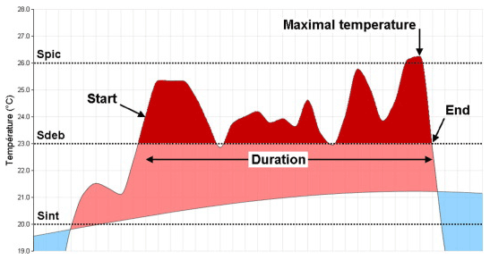
Figure 4 Figure and legend from Ouzeau et al. (2016): characterisation of a heatwave from a daily mean temperature indicator over France (example of a time series from 30 June to 5 August 1983). Duration (start and end), maximal temperature, and global intensity (red area of the plot). Temperatures above (below) the climatological line (1981–2010 reference period) are represented by the pink (blue) area. (For an interpretation of the references to colour in this figure legend, the reader is referred to Ouzeau et al., 2016).

3 The data set

3.1 Data availability

The data described in this article can be freely accessed on the Zenodo open-access repository: https://doi.org/10.5281/zenodo.5606983 (Doutreloup and Fettweis, 2021). As the files are numerous, each zipped folder contains all the data for each city concerned with this data set.

3.2 Structure of each file

All files are in a CSV format and are comma-separated. The file names are formatted in such a way that they contain all the information about the origin of the file. Each file name is composed as follows:

• for TMY or XMY: CityName_Type_Period_Scenario_MARmodel_ClimaticParameter.csv;

• for heatwaves: CityName_Type_Period_Scenario_MARmodel.csv;

with

• city name: the name of the city considered in this file;

• type: the nature of this file, namely, TMY (typical meteorological year), XMY (extreme meteorological year), HWE-HI (most intense heatwave event), HWE-HT (warmest heatwave event), HWE-LD (longest heatwave event), and HWE-all (all heatwave events);

• period: the time period considered;

• scenario: the IPCC scenario of the ESM considered, namely, “hist”, “SSP5-8.5”, “SSP3-7.0”, and “SSP2-4.5” (note that for MAR-ERA5, the name of the scenario is set by default to “hist” even if the ERA5 forcing does not contain any scenario);

• MAR model: the version of MAR used, namely, MAR-ERA5, MAR-BCC, MAR-MPI or MAR-MIR.

For TMY and XMY files, the header is composed of the task number (which is a reference number for internal use in the OCCuPANt project), the name of the city, and the name of the different variables accompanied by their unit. For HWE files, the header is composed of the task number (same remark as above), the name of the city, the characterisation of the heatwave (longest, warmest, and most intense) accompanied by its period, and the name of the different variables accompanied by their unit. Then comes the weather data with the time variable in the first column. Weather data are in universal time and leap year mode for the MAR-ERA5 and in no-leap year mode for MAR-BCC, MAR-MPI, and MAR-MIR.

A short example of how to select the desired data and files, as well as an example of how to use them, is provided in Appendix A for Liège-City.

4 Conclusion

The goal of this data set is to provide formatted and adapted meteorological data for specific users who work in building designing, architecture, building energy management systems, modelling renewable energy conversion systems, or other people interested in this kind of data. These weather data are derived from the regional climate MAR model. This regional model, adapted and validated over Belgium, is forced by a reanalysis and three ESMs. On the one hand, MAR is forced by the ERA5 reanalysis to represent the closest climate to reality. On the other hand, MAR is forced by three ESMs from the CMIP6 database, namely, BCC-CSM2-MR, MPI-ESM.1.2, and MIROC6. The main advantage of using the MAR model is that the generated weather data at a high resolution are spatially and temporally homogeneous.

The generated weather data follow two protocols. Firstly, the TMY and XMY meteorological data are generated largely inspired by the method proposed by the standard ISO15927-4, allowing the reconstruction of typical and extreme years, while keeping the plausible variability of the meteorological data. Secondly, the meteorological data concerning heatwaves (HWE) are generated according to the method proposed by Ouzeau et al. (2016) to detect the heatwave events and classify them according to three criteria of the heatwave. The OCCuPANt project, in which this paper is included, aims to identify the highest temperature, the longest heatwave duration, and the most intense heatwave event. Finally, all generated weather data are open source and freely available on the open repository Zenodo (https://doi.org/10.5281/zenodo.5606983, Doutreloup and Fettweis, 2021).

Appendix A: Example for Liège city

The Liège folder contains 596 files. This is a huge amount of files, so to find your way around, we suggest the following method for TMY and XMY files:

1. choose a typical or extreme year, i.e. select XMY for an extreme year;

2. choose the parameter that determines the typical or extreme year (TT for temperature and SWD for incoming solar radiation), i.e. if you want a year with extreme incoming solar radiation (i.e. sunshine), you should select SWDbased;

3. choose the reference period, i.e. 2085–2100 for the end of the century;

4. choose the socio-economic scenario, i.e. “ssp585” for a world that continues to use fossil fuels according to the SSP5-8.5 scenario;

5. choose one of the 3 MAR models, i.e. MAR-BCC for the MAR model forced by BCC-CSM2-MR;

6. finally, the choice is made for the file:

   Liège-City_XMY2085-2100_ssp585_MAR-BCC_SWDbased.csv.

This file selection method is a proposal, but each user is free to develop their own method and, of course, the user can use several files to compare them. For example, if the user wants to compare typical and extreme temperatures for the end of the century and for the two selected parameters with MAR-BCC, the user gets Fig. A1. Figure A1 clearly shows that the extreme year temperature based on temperature is much higher than the typical year temperature. On the other hand, the extreme year temperature based on incoming solar radiation is much lower – especially in January – than the typical year temperature, because extreme radiation in winter usually means cold weather.

Table A1 Full name, abbreviation name, lead institution, and references of the Earth system model (ESM) used in this study.

The method is almost identical for the heatwave files, except that there are no parameters to determine the typical and extreme years; instead, the user has to choose if they want to look at the longest, the most intense, the hottest, or all heatwaves present within the period. Therefore, if the user wants to compare the longest heatwave (HWE-LD) over the same period and for the same model and scenario as the example above, the user must choose the file: Liège-City_HWE-LD_2085-2100_ssp585_MAR-BCC.csv

Figure A2 compares the temperature evolution during the warmest heatwave, obtained from each of the MAR-BCC, MAR-MPI, and MAR-MIR simulations. The header of each file shows the warmest daily average temperature, namely, 37.2 ^∘C for MAR-BCC, 35.3 ^∘C for MAR-MPI, and 37.8 ^∘C for MAR-MIR. However, it can be seen in Fig. A2 that the hourly temperatures obviously rise much higher than these daily average values and, in this case, rise to ∼ 44 ^∘C for MAR-BCC and MAR-MIR, and ∼ 42 ^∘C for MAR-MPI.

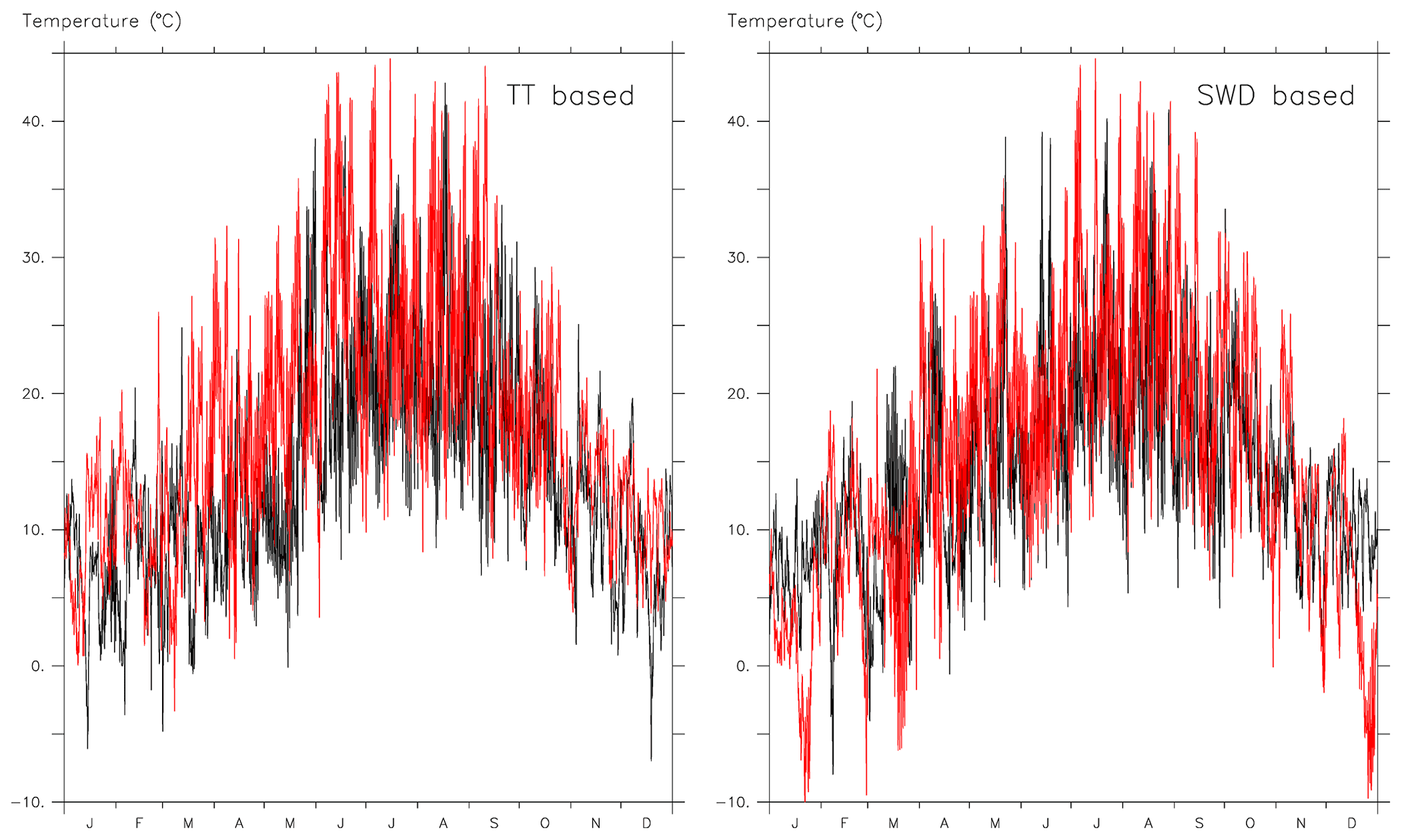
Figure A1 Typical (black) and extreme (red) temperature for Liège city, simulated by MAR forced by BCC-CSM2-MR, with the scenario SSP5-8.5 for the period 2085–2100. The typical/extreme months are based on temperature (left) and incoming solar radiation (right). These data are extracted from these files: Liège-City_TMY2085-2100_ssp585_MAR-BCC_TTbased.csv, Liège-City_XMY2085-2100_ssp585_MAR-BCC_TTbased.csv, Liège-City_TMY2085-2100_ssp585_MAR-BCC_SWDbased.csv, and Liège-City_XMY2085-2100_ssp585_MAR-BCC_SWDbased.csv.​​​​​​​

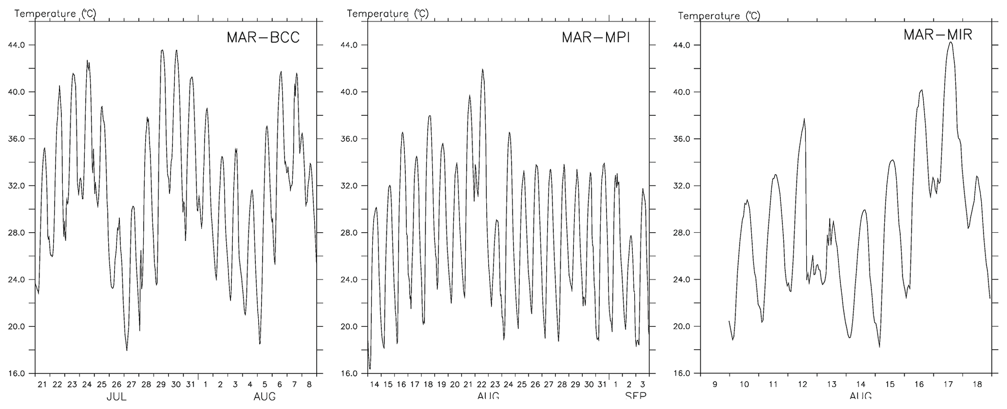
Figure A2 Temperature during warmest heatwave events for Liège city simulated by MAR-BCC (i.e. MAR forced by BCC-CSM2-MR), MAR-MPI (i.e. MAR forced by MPI-ESM.1.2), and MAR-MIR (i.e. MAR forced by MIROC6), with the scenario SSP5-8.5 for the period 2085–2100. These data are, respectively, extracted from these files: Liège-City_HWE-HT_2085-2100_ssp585_MAR-BCC.csv, Liège-City_HWE-HT_2085-2100_ssp585_MAR-MPI.csv, and Liège-City_HWE-HT_2085-2100_ssp585_MAR-MIR.csv.​​​​​​​