the Creative Commons Attribution 4.0 License.
the Creative Commons Attribution 4.0 License.
 | 27 Jan 2022
PAPILA dataset: a regional emission inventory of reactive gases for South America based on the combination of local and global information
Paula Castesana
Melisa Diaz Resquin
Nicolás Huneeus
Enrique Puliafito
Sabine Darras
Darío Gómez
Claire Granier
Mauricio Osses Alvarado
Néstor Rojas
Laura Dawidowski
The multidisciplinary project Prediction of Air Pollution in Latin America and the Caribbean (PAPILA) is dedicated to the development and implementation of an air quality analysis and forecasting system to assess pollution impacts on human health and economy. In this context, a comprehensive emission inventory for South America was developed on the basis of the existing data on the global dataset CAMS-GLOB-ANT v4.1 (developed by joining CEDS trends and EDGAR v4.3.2 historical data), enriching it with data derived from locally available emission inventories for Argentina, Chile, and Colombia. This work presents the results of the first joint effort of South American researchers and European colleagues to generate regional maps of emissions, together with a methodological approach to continue incorporating information into future versions of the dataset. This version of the PAPILA dataset includes CO, NOx, NMVOCs, NH3, and SO2 annual emissions from anthropogenic sources for the period 2014–2016, with a spatial resolution of 0.1∘ × 0.1∘ over a domain that covers 32–120∘ W and 34∘ N–58∘ S. The PAPILA dataset is presented as netCDF4 files and is available in an open-access data repository under a CC-BY 4 license: https://doi.org/10.17632/btf2mz4fhf.3 (Castesana et al., 2021). A comparative assessment of PAPILA–CAMS datasets was carried out for (i) the South American region, (ii) the countries with local data (Argentina, Colombia, and Chile), and (iii) downscaled emission maps for urban domains with different environmental and anthropogenic factors. Relevant differences were found at both country and urban levels for all the compounds analyzed. Among them, we found that when comparing PAPILA total emissions versus CAMS datasets at the national level, higher levels of NOx and considerably lower levels of the other species were obtained for Argentina, higher levels of SO2 and lower levels of CO and NOx for Colombia, and considerably higher levels of CO, NMVOCs, and SO2 for Chile. These discrepancies are mainly related to the representativeness of local practices in the local emission estimates, to the improvements made in the spatial distribution of the locally estimated emissions, or to both. Both datasets were evaluated against surface concentrations of CO and NOx by using them as input data to the WRF-Chem model for one of the analyzed domains, the metropolitan area of Buenos Aires, for summer and winter of 2015. PAPILA-based modeling results had a smaller bias for CO and NOx concentrations in winter while CAMS-based results for the same period tended to deliver an underestimation of these concentrations. Both inventories exhibited similar performances for CO in summer, while the PAPILA simulation outperformed CAMS for NOx concentrations. These results highlight the importance of refining global inventories with local data to obtain accurate results with high-resolution air quality models.
- Article
(2850 KB) - Full-text XML
- BibTeX
- EndNote


South America (SA) is a region of complex political and social contrasts, fluctuating economies, and the highest inequality levels worldwide (The World Bank, 2019). Demographically, SA is a region with a growing population and an increasing trend towards urban agglomeration and the demand for goods and services (Huneeus et al., 2020a). Regarding energy use, SA has significantly low coal consumption levels and a higher share of hydroelectricity in comparison with other world regions (IEA, 2020). The use of alternative fuels, such as biomass or waste, is usually not well covered by national statistics, and therefore global information does not accurately represent the sectoral mix of fuels consumed in the different countries. Road transport in the region is characterized by a fleet older and in poorer operating and maintenance conditions than that circulating in developed countries. Moreover, the use of motorcycles has increased in the region, being of particular concern in some cities such as Lima and Bogotá (Romero et al., 2020; Ortegon-Sanchez and Oviedo Hernandez, 2016). In addition to diesel oil and gasoline, different fuels are consumed for road transport in the region: compressed natural gas (CNG) covers a significant fraction of fuel use by passenger vehicles in Argentina, a high share of liquefied petroleum gas (LPG) is used in Peru, while pure ethanol and gasoline–ethanol blends are broadly used by flex fuel vehicles in Brazil (Belincanta et al., 2016). Adding to this diversity, legislation on sulfur content in fuels is very restrictive in some countries such as Chile and Colombia and much more flexible, particularly concerning diesel oil used by trucks and off-road vehicles, in others (Huneeus et al., 2020a). With respect to land use, SA is one of the least densely populated places in the world, although it is highly urbanized (United Nations, 2015). This often implies poor or lacking information on the level and spatial distribution of some anthropogenic activities. This is the case, for example, for the extended use of wood and waste for cooking and for heating in colder zones of the region, e.g., southern Chile (Villalobos et al., 2017). Another relevant land use characteristic is the sustained trend of increasing harvested land areas largely due to conversion from forests to agricultural lands (The World Bank, 2020), and partly as a consequence of rising temperatures and changes in rainfall patterns, resulting in a shift of the agricultural border as has occurred in Argentina (Barros and Camilloni, 2016). Lastly, a unique feature of the region concerns hotspots of sulfur dioxide identified by the Ozone Monitoring Instrument (OMI) satellite sensor. For SA they are attributable mainly to volcanoes and the smelting of sulfides of copper and other metal ores in Chile and Peru, differing remarkably from other regions worldwide where these hotspots are mainly emitted by thermal power plants and oil and gas activities (Fioletov et al., 2016).
These regional particularities have direct consequences not only on the level and chemical profiles of the pollutants discharged to the atmosphere, but also on the specific locations where these emissions occur and on the population exposed to their environmental and health effects. Assessing the impact of atmospheric emissions as well as designing mitigation strategies requires reliable atmospheric emissions inventories (AEIs), which include spatially disaggregated emissions covering the entire region of interest in a transparent and consistent way in terms of emission sources and estimation methodologies (Kuenen et al., 2014). There is a wide range of global AEIs covering SA for different species and periods that meet the mentioned requirements. Some of the AEIs worth mentioning include the Emissions Database for Global Atmospheric Research (EDGAR) (Janssens-Maenhout et al., 2019; EDGAR, 2021), the Evaluating the Climate and Air Quality Impacts of Short-Lived Pollutants (ECLIPSE) (Stohl et al., 2015), the Community Emissions Data System (CEDS) (Hoesly et al., 2018), the integrated assessment model Greenhouse gas – Air pollution Interactions and Synergies (GAINS) (Klimont et al., 2017), or the Copernicus Atmosphere Monitoring Service datasets (CAMS) (Granier et al., 2019).
Across the region, government efforts on AEIs are mainly focused on greenhouse gases (GHGs) in line with the international commitments under the United Nations Convention on Climate Change (UNFCCC). The regional community of GHG inventory compilers has grown remarkably in the last 2 decades and in many cases has helped to improve the collection of activity data including specific areas of national statistics systems. In parallel, research groups in SA have built inventories of ozone precursors and particles to be used as input data to air quality models. Links between several of these groups have recently been strengthened by the creation of a regional initiative focused on the construction of inventories of species not covered by governments in their reports to the UNFCCC (Huneeus et al., 2017, 2020a).
Completeness in terms of species, represented sectors, and time series is a strength of global AEIs while locally developed inventories seldom fully cover all three aspects. On the other hand, although the most current versions of global AEIs accurately reflect the emissions from sectors for which regional information is well documented in global statistics, they may miss some specificity and accuracy associated with local practices and technologies that are often better represented in local AEIs (Huneeus et al., 2020a). From this, it is plausible to assume that better emission estimates would be obtained by enriching the comprehensive global AEIs with locally generated information. This mosaic approach is an idea that has been successfully applied in the framework of the Task Force on Hemispheric Transport of Air Pollution (HTAP), an international cooperative effort to improve the understanding of the intercontinental transport of air pollution across the Northern Hemisphere. In this context, the HTAP_v2.2 air pollutant grid maps were developed combining available regional information within a complete global dataset (Janssens-Maenhout et al., 2015) and have been widely used even outside of HTAP.
This work presents what to our knowledge constitutes the first AEIs from anthropogenic sources covering the continental SA region, which combines local available information with a global database in a proper and rigorous way. For this purpose, the dataset CAMS-GLOB-ANT v4.1 (Granier et al., 2019), developed by joining CEDS trends and EDGAR v4.3.2 historical data, was used as a basis (hereinafter CAMS dataset), enriching it with locally developed inventories available in the literature until 2019 and selecting those with national coverage and with availability of data for the period and species of interest. The dataset presented in this work, hereinafter called PAPILA, focuses on the group of species known as reactive gases, given their relevance in atmospheric chemistry as precursors of O3 and PM2.5: carbon monoxide (CO), nitrogen oxides (NOx), non-methane volatile organic compounds (NMVOCs), ammonia (NH3), and sulfur dioxide (SO2) (Sharma et al., 2017). Due to the availability of data in the local AEIs and the completeness of the sectors represented, the 2014–2016 period was selected for this first version of the PAPILA dataset, including local information from the continental areas of Argentina (Puliafito et al., 2017; Castesana et al., 2018), Chile (Mazzeo et al., 2018; Gallardo et al., 2018), and Colombia (IDEAM, 2017). In addition, a comparison of the performance of both AEIs (PAPILA and CAMS) is presented using near-surface CO and NOx mixing ratios simulated by the Weather Research and Forecasting-Chemistry (WRF-Chem) model (Grell et al., 2005) at a high spatial resolution (3 km) against in situ observations made in Buenos Aires during February–March and August–September 2015.
This work was carried out within the framework of the Prediction of Air Pollution in Latin America and the Caribbean (PAPILA, 2020) and Emission Inventories in South America (EMISA, 2020) projects. PAPILA combines, for the first time, an ensemble of state-of-the-art models, high-resolution emission inventories, space observations, and surface measurements to provide real-time forecasts and analysis of regional air pollution in the Latin American and the Caribbean regions. Thus, an important aspect of the project is the development of appropriate and consistent surface emission inventories as input data for air quality models. The EMISA initiative was created to lay the foundations for constructing robust and transparent inventories of the same set of species that have been consistently estimated across South American countries using the same methodological approach. Local information on emissions was gathered from the countries that participate in the EMISA project: Argentina, Brazil, Chile, Colombia, and Peru. Relevant research groups in Brazil and Peru have developed emission inventories for different cities (Policarpo et al., 2018; Dos Santos Lucon and Moutinho Dos Santos, 2005; Vivanco and Andrade, 2006; Romero et al., 2020; Dawidowski et al., 2014); however as far as we know they have not developed inventories covering the entire countries for the species included in this study. Since national territories are the common administrative entities that can be exchanged with the global inventory, the local information on emissions from these countries was not included in this first version of the combined dataset. However, this work is expected to be the starting point for the preparation of comprehensive emission inventories in South America enriched with local information. For this purpose, we include a flow chart with the general methodology that we have applied in combining local information with a global dataset.
The paper is organized as follows. Section 2 describes, for each country, the approach and sources of information used to develop the PAPILA dataset and also discusses the application of this inventory in an air quality model. Section 3 provides the main differences of PAPILA and CAMS datasets for SA and other smaller domains and the results of the air quality simulations. Section 4 provides a description of the data availability, and finally Sect. 5 presents the main conclusions of this work.
2.1 PAPILA dataset overview
The PAPILA dataset is a collection of CO, NOx, NMVOCs, NH3, and SO2 inventories of annual emissions from anthropogenic sources in South America for the period 2014–2016. The inventories are presented as netCDF4 files, one for each species gridded with a spatial resolution of 0.1∘ × 0.1∘ covering the domain 32–120∘ W and 34∘ N–58∘ S. Each file contains 12 variables corresponding to the emissions in Tg yr−1 from the following categories, which are organized and denominated using the nomenclature given by CAMS: thermal power plants (ENE); residential and commercial combustion (RES); road transportation (TRO); non-road transportation (TNR); fugitive emissions (FEF); industries, including fuel consumption in manufacturing industries and construction, refineries, industrial processes, and solvent and other product use, (IND); agricultural soils (AGS); agricultural livestock (AGL); domestic and international navigation (SHP); waste (including solid waste, wastewater, and incineration) (SWD); and the sum of all categories (SUM). This grouping of categories was carried out following the CAMS sectoral disaggregation, except for the use of solvents, reported under IND in the PAPILA dataset. To be consistent with the base inventory (CAMS-GLOB-ANT v4.1) used for our mosaic inventory, aviation emissions were not included in this first version of the PAPILA dataset. Agricultural fires were removed to allow the use of the inventories together with fire products such as GFEDv3 (van der Werf et al., 2010), FINN v1 (Wiedinmyer et al., 2011), and GFAS v1 (Kaiser et al., 2012), avoiding double counting of these fires. It is worth mentioning that by “sum of all categories” we refer to all those included in PAPILA, both for the presentation of our results and for comparative purposes with CAMS. A broader description of the activities contemplated under each category is presented in Table A1 in Appendix A, together with the equivalences with the IPCC 1996 reporting code.
The PAPILA dataset (Castesana et al., 2021) combines surface emissions from the comprehensive CAMS dataset with local information of those countries that, at the time of development of this emission inventory, had emission estimates of the mentioned species and covering the entire national territory: Argentina, Chile, and Colombia. That information was collected and assessed in terms of species, emission categories, and spatial coverage, selecting the most appropriate and representative data for each country, as described in the following subsections and summarized in Fig. 1.
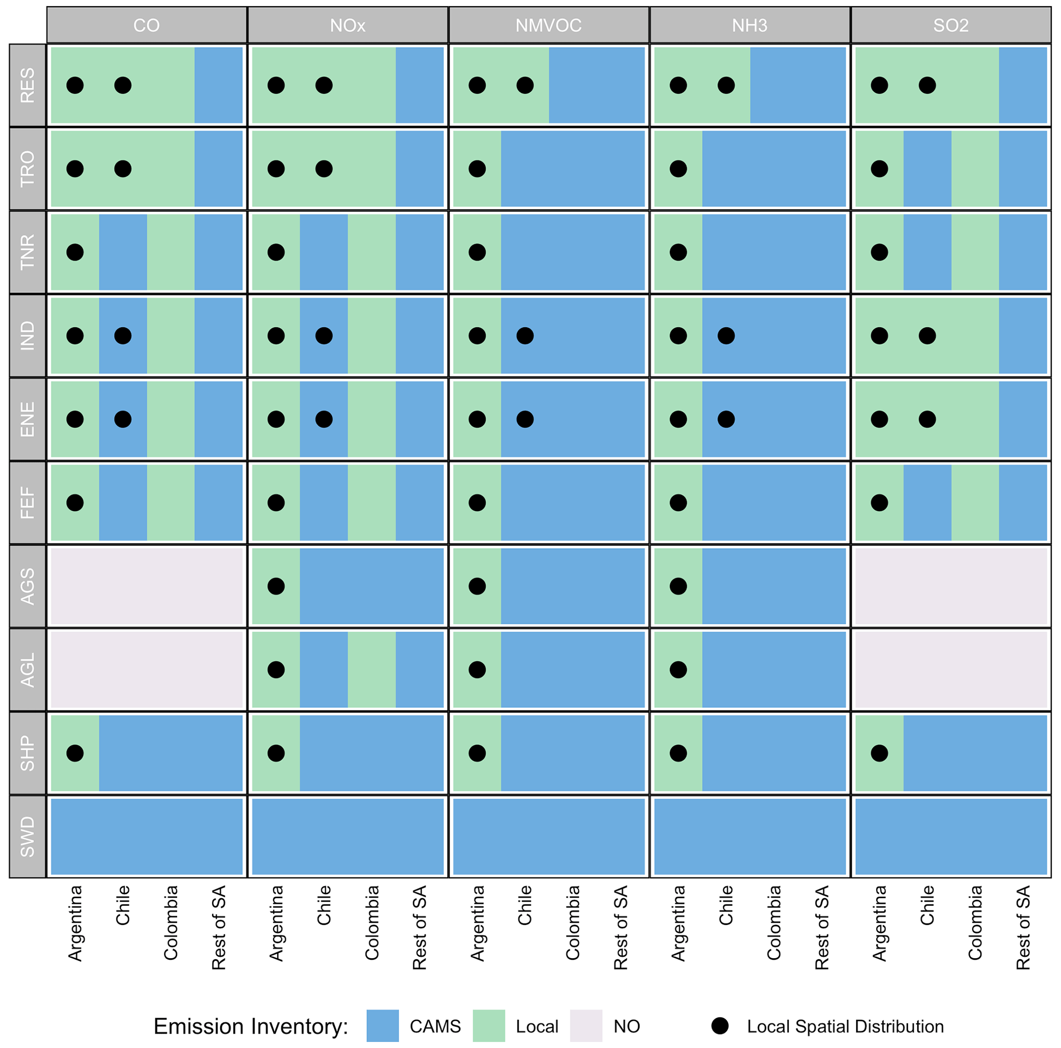
Figure 1Local and global information on emissions and their spatial disaggregation included in the PAPILA dataset, by species, category, and country. ENE: thermal power plants; RES: residential, commercial, and other combustion; TR: road transportation; TRN: non-road transportation; FEF: fugitive emissions; IND: industrial process; AGS: agricultural soils; AGL: agriculture livestock; SHP: domestic and international navigation; SWD: waste. CAMS refers to the global dataset CAMS-GLOB-ANT v4.1, and “Rest of SA” refers to the rest of the countries of the South American region. NO: not occurring.
2.2 Designing and building the PAPILA dataset
Figure 2 presents a flow chart of the general methodology applied in combining local information with CAMS. Data from Argentina, Chile, and Colombia were assessed in terms of species availability. In addition, and as described in the next subsections, the transparency on the methodology applied in emission estimates and the representativeness and completeness of emission categories were revised in line with the CAMS emission reporting system. For those species and/or categories with an absence of local data, the CAMS inventory was used to fill the gaps.
One of the challenges of combining different local inventories into a common regional database is bringing them to a single, uniform, and homogeneous grid. For this purpose, it was necessary to resolve all conflicts arising from cells shared by more than one country or coastal cells. To be consistent with the base inventory used in this work, this problem was solved using the country and continent masks applied by CAMS (CIESIN and CIAT, 2005), which are created at 0.1∘ resolution assigning a unique country value for each cell.
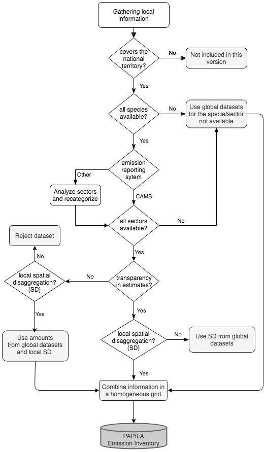
Figure 2Flow chart illustrating the general methodology applied to combine local information with the global dataset CAMS-GLOB-ANT v4.1.
2.2.1 Argentina
Spatially disaggregated emission inventories for all the species included in this work are available for Argentina. They cover all categories except SWD. Emissions from the categories ENE, RES, TRO, TNR, FEF, IND, and SHP were taken from the GEAA inventory (Puliafito et al., 2017), which consists of a high-resolution (0.025∘ × 0.025∘) inventory of 2014 annual emissions. For each category, GEAA covers
-
(i) for energy industries the precise location of power plants, plus fuel consumption by technology and by fuel of each utility;
-
(ii) for residential and commercial sources spatially distributed fuel consumption estimated using energy use by province and census-based population maps;
-
(iii) for road transportation fleet composition and fuel consumption by refueling stations, geographically distributed considering road maps by type and distance to the refueling stations;
-
(iv) for off-road transportation emissions from railways, with fuel consumption data, geographically distributed with rail maps;
-
(v) for fugitive emissions including those from refining, storage, venting, and flaring and those from distribution of oil products and natural gas, annual data from national statistics, spatially distributed with the exact location of the facilities;
-
(vi) for inland navigation (namely, domestic plus international navigation on the continental area of Argentina) fuel consumption spatially distributed with the geographical identification of the berths, routes and port boundaries.
The GEAA inventory has been updated for this work including emissions from IND, which were not covered in the published version (Puliafito et al., 2017). These emissions include (i) those from fuel consumption and from the production process itself for the main industries, disaggregated by fuel and spatially distributed with the precise location of each facility, and (ii) those from fuel consumption of small industries, whose consumption is known by activity and by district, and whose spatial disaggregation of emissions was carried out using the population density of each district as a proxy. We noted that a different allocation of fugitive emissions from the distribution of oil products and natural gas (mainly consisting of NMVOCs) exists between CAMS and the Argentinean inventory: CAMS includes these emissions under the IND category (see Table A1, Appendix A) while they are reported under FEF in the Argentinean inventory. This does not imply omission or double counting of emissions.
To construct the PAPILA inventory, this new version of GEAA was updated to 2015 and 2016 by applying CEDS trends by emission categories. Final emissions were adapted to a homogeneous grid of 0.1∘ × 0.1∘ and combined with local agricultural inventories described below and with the CAMS information on emissions from SWD and from SHP outwards from the Argentine coast.
Ammonia emissions from agricultural activities were taken from the 2000–2012 estimates by Castesana et al. (2018). The time series was updated to the period 2014–2016 by applying the methodology and local activity data sources detailed in the cited work. The rest of the studied species emitted from activities under AGL and AGS (i.e., NOx and NMVOCs) were estimated according to the 2016 methodology of the European Monitoring and Evaluation Program (EMEP, 2017), following the general expression
where Ei is the emission amount of the species i, AD is the activity data, and EFi represents the emission factor of the species i related to that activity. Both the activity data and their spatial distribution were based on the previous work by Castesana et al. (2018, 2020), while the emission factors were those suggested by the EMEP according to the level of detail described for each activity in Table 1. These emissions have been estimated ad hoc to be included as part of the PAPILA dataset. Since they have not been published thus far, interested readers may find a more complete description of the results in Appendix A, including resulting emissions from fertilizers, crop production, and animal excreta (dairy and beef cattle, poultry, swine, sheep, goats, horses, and other livestock). Consistent with the referenced studies cited above, emissions from managed excreta are reported as AGL, and those deposited in pasture during animal grazing are reported under AGS. Resulting inventories of annual emissions from agricultural activities spatially disaggregated at the district level were converted to grids with a 0.1∘ × 0.1∘ resolution.
Table 1Level of detail of the EMEP 2016 methodology applied in estimating NOx and NMVOC emissions from agricultural activities in Argentina.

* There is no EMEP Tier 2 method. Emissions from grazing (deposited on pasture) are reported as agricultural soils. NO: not occurring. AGS: agricultural soils. AGL: agricultural livestock.
2.2.2 Chile
Annual Chilean emissions were taken from the CR2-MMA dataset (CR2-MMA, 2018), based on the works of Gallardo et al. (2018) and Mazzeo et al. (2018). This dataset is presented with a spatial resolution of 0.01∘ × 0.01∘ and includes 2014 emissions of reactive gases, GHGs, and particles, reported under the following aggregation: industries (which include emissions from energy), urban and non-urban road transportation (which only includes CO and NOx for reactive gases), residential consumption, and agricultural and forest fires.
Emission from industrial sources corresponds to the compilation of self-declared estimates by each facility to the Chilean Repository of Emissions and Pollutants Transport. Neither the methodology nor the emission factors used to estimate these emissions could be traced. For the particular case of SO2, the local methodology for the emission estimates is based on sulfur content in fuels and in mass balances in copper production processes, which constitute the main SO2 emitter activity in Chile (González-Rojas et al., 2021). For this reason, and assuming that the information on sulfur content handled locally is reliable, we have included the spatially distributed emissions as estimated in Chile in our dataset. For the rest of the species, we decided to exclusively adopt the spatial distribution and the share of the locally reported emissions and distributed the CAMS estimates by weighing them on the CR2-MMA spatial distribution as follows:
where represents the emissions of species i and category j assigned to the cell grid k, N is the total number of grid cells covering the country, Elocal represents the emissions locally estimated, and ECAMS is the corresponding estimate from the global database.
Emission estimates from residential sources in the CR2-MMA dataset cover only firewood combustion for all species considered in our work (Mazzeo et al., 2018). According to local experts, one of the most relevant aspects of air quality in the coldest regions in southern Chile is the presence of CO, NMVOCs, and particles from burning of firewood in households. Although this practice is included under the residential category of global inventories, the corresponding estimated emissions do not seem to be consistent with the magnitude of the air pollution situation observed at the local level (Huneeus et al., 2020b). In addition, by downscaling global inventories in the metropolitan region of Santiago (Chile's central region), Huneeus et al. (2020a) found out that residential emissions were strongly overestimated in global databases and attributed this inaccuracy to the use of population density as a proxy for the spatial distribution. Residential emissions from firewood burning are less relevant in the more temperate northern areas where air pollution is mostly linked to emissions of SO2 and particles from the metal industry (Huneeus et al., 2020b). From this and assuming that (i) residential firewood burning is a predominant source in the southern region and (ii) in central and northern regions this work improves the representation of the diversity of sources and local practices for the other fuel combustion categories, we have decided to replace the residential emissions of CAMS with those of the CR2-MMA, at the risk of underestimating residential emissions in the central and northern regions by omitting those from fuels other than firewood (see Sect. 3.1).
Local estimates of CO and NOx emissions from urban and non-urban road transportation were aggregated and reported in the PAPILA dataset under the TRO category. Given that the magnitudes and the spatial distribution of emissions from ENE and IND (including use of solvent) are reported in an aggregate way in the Chilean inventory, we decided to report them under the IND category. Emissions taken from CR2-MMA were extrapolated to 2015 and 2016 by applying CEDS trends (Hoesly et al., 2018) and projected to a 0.1∘ × 0.1∘ grid. Emissions from categories and species not estimated by the local inventory were taken from the CAMS inventory.
2.2.3 Colombia
For the purpose of the PAPILA dataset, the only available information for Colombia was the emission estimates of CO, NOx, and SO2 at the national level from all the categories of interest, except agricultural soils. These estimates were developed for the Third National Communication of Colombia to the UNFCCC, covering the period 2010–2014 (IDEAM, 2017). Annual emissions from Colombia were extrapolated to 2015 and 2016 by applying linear regression forecast using the local time series and disaggregated using the spatial distribution of sources of the CAMS inventory as follows:
where variables and indexes are those described in Eq. (2).
Although in this context the country reports CO, NOx, and SO2 emissions from SWD, CAMS reports them as zero. The latter precluded the spatial assignment of the locally estimated emissions, and for this reason it was decided to take the SWD category from CAMS.
2.3 Comparison of local and global datasets
A spatial analysis was performed following a similar approach to Trombetti et al. (2018) in their work on spatial inter-comparison of top-down emission inventories in European urban areas, in which the analysis was made in terms of normalized emission values by a group of categories and for different urban domains in order to become independent of emission levels and to show the relative contribution of a certain group of emission activities in different areas. Since in our work we are interested in comparing only two inventories without losing sight of the differences in terms of magnitude, we have adapted this approach by comparing normalized emissions by category and urban domain, normalizing them with respect to those from the CAMS dataset, as shown in Eq. (4). In this way, we were able to compare both datasets in relative terms and without losing information on the shares of each group of categories and the differences in the emission levels of each dataset.
where and are the normalized emissions and the emission levels, respectively, of the species i and group of categories J corresponding to the dataset d and the area (region, country, or urban domain) covered by the total number N of cell grids k.
For this analysis, we grouped categories as ENE + IND, RES, TRO, and “others”, and applied the analysis to (i) the SA region, (ii) countries with local data (Argentina, Chile, and Colombia), and (iii) urban domains from those countries that have implemented their own methodologies for the spatial distribution of emissions. Urban domains were selected seeking to represent a wide variety of environmental and anthropogenic factors. In Chile, we have chosen three regions with different air quality concerns: Antofagasta (northern region) with a strong presence of mining activity; Osorno (southern region), a cold region where firewood burning dominates residential emissions; and the metropolitan region of Santiago (central region, hereinafter Santiago) with a mix of emission sources and a strong presence of road transport. In Argentina, we have chosen three urban domains where relevant research groups are located, hoping that this analysis would contribute to these activities. Those sites are the metropolitan area of Buenos Aires (to facilitate reading, hereinafter Buenos Aires), which is a coastal city and one of the main megacities in South America; Bahía Blanca (B. Blanca), which is a port city with an important industrial park; and Mendoza, one of the most important cities in the country that borders the Andes mountain range. A broader description of the studied areas is included in Table A3 and Fig. A1 of Appendix A.
2.4 WRF-Chem simulations: case study in Buenos Aires
The performance of the PAPILA dataset in comparison with CAMS can be assessed using both inventories as input data of a regional model, implemented in the whole domain where local data have been integrated into the global dataset. This vast region, which includes the tropical Andes in Colombia, the dry Andes in southern Chile, and the Argentinean plateau towards the Atlantic coast, is characterized by diverse topographic features and vegetation patterns. In order to capture the differences in boundary layer process and surface energy budget in the whole area, a high-resolution model is needed, set up in each area where the main changes between the PAPILA and CAMS datasets have been made. As a first step of this verification exercise, here we present a study focused on Buenos Aires, using the Weather Research and Forecasting Chemistry regional model version 4.1.2 (WRF-Chem v4.1.2). This megacity is strongly influenced not only by mobile and residential sources, but also by the presence of four big thermal power plants, an important industrial park, and an international port. Simulations were conducted using the model over three nested domains with the highest horizontal resolution of 3 km centered in Buenos Aires. Two time periods were selected to cover summer (from 7 February to 5 March 2015) and winter (from 26 August to 17 September 2015) to assess the role of the emission estimates from the two inventories in the simulated air pollutant concentrations in the different seasons.
2.4.1 Model description and simulation configuration
WRF-Chem is a fully coupled online chemistry transport model that simultaneously predicts weather and atmospheric composition (Grell et al., 2005). The simulations were done over three nested domains. The lowest-resolution domain (d01) has a grid size of 18 km × 18 km (15–57∘ S, 51–78∘ W), and the highest-resolution domain (d03) has a 3 km × 3 km grid covering the metropolitan region of Buenos Aires and the surroundings. The coverage of the domains can be seen in Fig. A2. All the simulations conducted in this study were performed using a spin-up time of 2 weeks.
Lambert-conformal projections were used. The physical parameterizations adopted for the three domains were (a) the Thompson scheme (Thompson et al., 2008) for microphysics, (b) the Grell 3D scheme for cumulus parameterization, (c) The Yonsei University scheme for boundary layer processes, (d) the MM5 similarity scheme for surface processes, and (e) the RRTMG scheme to compute long- and shortwave radiation. The chemistry in these simulations was modeled using the GOCART bulk aerosol scheme for aerosol-phase chemistry along with RADM2 for gas-phase chemistry. The initial and boundary conditions were taken from the NCEP Final Operational Global Analysis data (FNL), available at a resolution of 1∘ every 6 h (NOAA, 2000).
The FINN fire database was used for fire emissions (Wiedinmyer et al., 2011), the MEGAN biogenic database was used for biogenic emissions (Guenther et al., 2006), and sea salt emissions from GOCART were also included.
Reported annual emissions in 2015 from the two inventories were processed to produce hourly-resolved emissions at the resolution of each of the domains. Since the PAPILA dataset only includes reactive gases, for aerosol emissions the ones of the CAMS simulation were used: EDGAR v4.3.2 global emission database for PM2.5 and PM10 and CAMS v4.1 for organic carbon (OC), BC, and volatile organic compounds (VOCs). However, the results presented in this article will only cover the species included in the PAPILA inventory.
For ENE, TRO, and RES, monthly emission patterns were defined to breakdown total annual emissions into monthly fluxes (see Fig. A2). Emissions from other categories were evenly distributed throughout the year. The RES monthly cycle was established from the reports on natural gas consumption reported in national statistics (ENARGAS, 2021) for residential and commercial activities in Buenos Aires. This profile shows a maximum during winter linked to the increase in residential heating. Similarly, the TRO monthly cycle was defined from the total fossil fuel consumption from the road transport reported in the statistics for the entire country (Secretaría de Energía, 2021). For ENE, the same source of data was used to obtain monthly fossil fuel sales for thermal power plants in Buenos Aires Province. Weekly cycles taken from PREP-CHEM (Freitas et al., 2011) were applied to the resulting total monthly emission fluxes. The diurnal cycles were adapted from those reported by Wang et al. (2010), focusing on reproducing Buenos Aires traffic patterns observed in the two monitoring stations: Parque Centenario and Córdoba. With this approach, the best configuration obtained with the simulations includes 3-hourly emission patterns: one related to diesel vehicle emissions, defined using PM observations, and the other associated with gasoline car emissions in winter and in summer, defined with the measured concentrations of CO and NOx.
2.4.2 Model evaluation
The highest-resolution model outputs using these two emission inventories were evaluated against CO and NOx ground-based observations from the available monitoring stations in Buenos Aires (see locations of the sites in Fig. A2). Air pollutant data from the Environmental Protection Agency of Buenos Aires (APRA) include hourly measurements of NOx and CO at two sites, Córdoba (34.60∘ S, 58.39∘ W) and Parque Centenario (34.61∘ S, 58.44∘ W). Córdoba's site is located in a commercial area with high vehicular flow and very low incidence of stationary sources while Parque Centenario is located in a residential area next to an arboreal space with medium vehicular flow and also very low incidence of stationary sources. As the air quality database is at an hourly resolution, the model was also sampled every hour.
The model evaluation was mainly focused on the effects of enriching the CAMS inventory with local inventories on the simulated air pollutant concentrations. For this purpose, median and percentiles for the entire period were evaluated. Also, mean daily concentrations were calculated to inspect whether model performance of both inventories was consistent and satisfactory. Well-accepted statistical measures such as normalized mean bias (NMB), normalized mean gross error (NMGE), and the fraction of predictions within a factor of 2 (FAC2) were used (Wang et al., 2021). These statistical metrics were calculated using the following expressions:
where Sk and Ok are the simulated and observed hourly average concentrations, respectively, and N is the total number of observations. The model was sampled at each measuring location using grid interpolation and compared with the ground-based observations for the calculation of statistical performance metrics.
Table 2 reports the resulting 2015 annual emissions of CO, NOx, NMVOCs, NH3, and SO2 corresponding to the sum of all categories in the PAPILA dataset, for different domains: South America, Argentina, Buenos Aires, Bahía Blanca, Mendoza, Chile, Santiago, Antofagasta, Osorno, and Colombia, in comparison with the corresponding emissions levels from CAMS. In addition, Fig. 3 depicts the shares of each group of categories (ENE + IND, RES, TRO, and others) to the total emissions of each species and for all the aforementioned domains. They are expressed in a normalized way with respect to the sum of all categories here analyzed in CAMS for each corresponding species and domain. In this way, the emissions of each species in CAMS correspond to the sum of the share of each group of categories, adding up to a total of 1.00. On the other hand, the shares of each category in PAPILA can be compared with those in CAMS and add up to a total greater or less than 1.00 according to the differences in the sum of all the categories indicated in Table 2.
The spatial distribution of 2015 annual emissions of CO, NOx, NMVOCs, NH3, and SO2 is shown in Fig. 4 for the sum of all categories. In addition, this figure includes maps with the differences between PAPILA and CAMS datasets for each species, depicting the differences in terms of intensity and location of emission sources. For comparative purposes, emissions from agricultural fires have been subtracted from the sum of all categories in the CAMS database.
In what follows results are presented firstly by species, highlighting the most relevant aspects of the 2015 emission (Sect. 3.1). Then, surface concentrations of CO and NOx obtained from the use of the PAPILA dataset as input information in a chemical transport model in Buenos Aires, compared to those obtained using CAMS, are presented (Sect. 3.2). The section ends with an analysis of the local aspects that may have generated the difference between both emission databases (Sect. 3.3).
Table 2Summary of annual emissions by domain for 2015 (Gg yr−1).
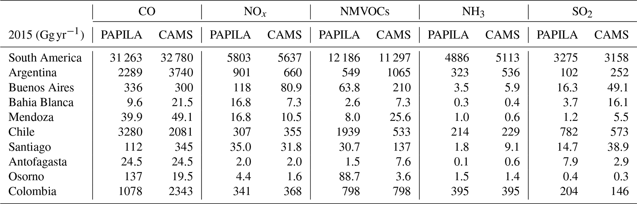
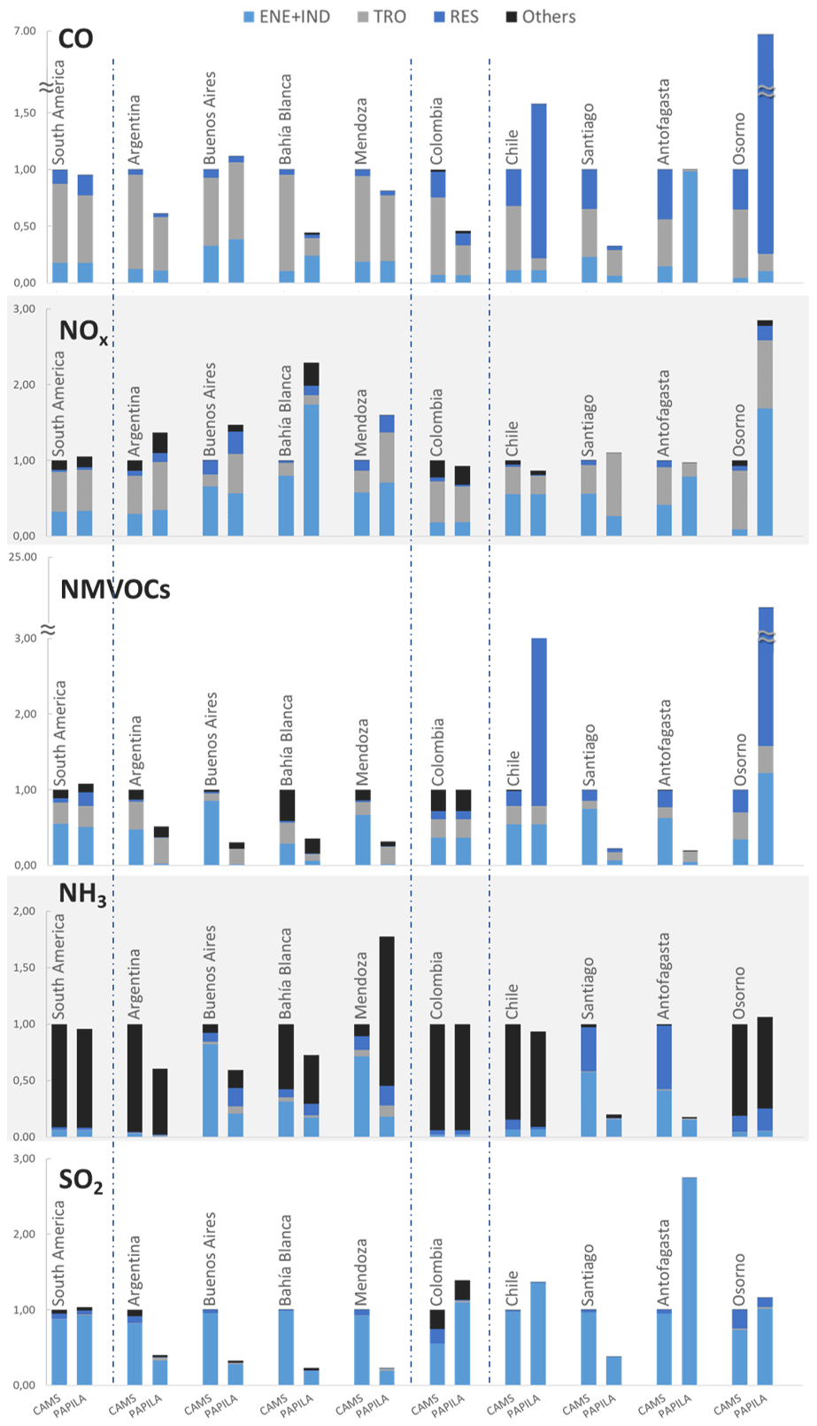
Figure 3Normalized breakdown of PAPILA emissions compared with the CAMS inventory by domain and category group for 2015. Total CAMS emissions for each domain equal to 1. ENE + IND: energy and industries; RES: residential and commercial combustion; TRO: road transportation; others: non-road transportation, fugitive emissions, agricultural soils, agriculture livestock, navigation, and waste.
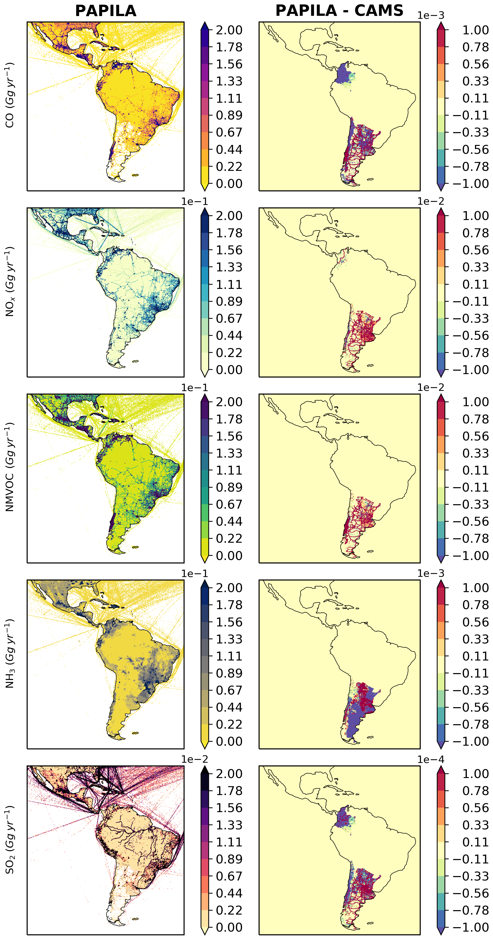
Figure 4(left) Spatial distribution of 2015 PAPILA emissions (Gg yr−1) and (right) difference between PAPILA and CAMS inventories by species in 2015.
3.1 Local–global comparison by species
3.1.1 Carbon monoxide
Local estimates of CO for Argentina and Colombia presented lower CO annual emissions than those in CAMS; the largest differences occurred under the TRO category. Although the local estimates for TRO in Chile also showed significantly smaller levels, this difference was masked in the total CO national estimates by the larger emissions from the residential category, even after having omitted CO emissions from fuel combustion other than firewood. Lower CO PAPILA emissions in Argentina (−39 %) and Colombia (−54 %) were compensated for by larger PAPILA emissions in Chile (58 %). According to the CAMS dataset these three countries are only responsible for 25 % of the total SA emissions, and hence the impact of the changes introduced in this work on total SA is very limited. This same situation occurs with the other species, for which it is found that these three countries are only responsible for 20 %–25 % in the case of NOx, NMVOCs, and NH3 and 31 % for SO2 (Table 2). However, when analyzing the impact on these three countries together, and even when these countries compensate for each other, a difference with CO CAMS emissions of −19 % is observed.
At the urban level, in the Buenos Aires domain PAPILA emission estimates were 12 % higher than those from CAMS; this difference was mainly associated with higher local emissions from TRO and ENE + IND, even with lower emissions from RES. In the same way, Mendoza and B. Blanca exhibited lower CO total levels, mainly associated with differences in TRO and to a lesser extent in RES. In B. Blanca, this difference masked the larger emissions by a factor of 5 in the local estimates of ENE + IND with respect to the global dataset. By downscaling the B. Blanca urban domain, we identified the absence of emissions from shipping activities in the global inventory. While emissions from SHP within the continental area were estimated locally, offshore emissions were taken from CAMS, which reports zero emissions for this region. In this domain, emissions from navigation activities are a concern since its port activity is almost as relevant as that of the international port of Buenos Aires (Ports, 2021). Although the absence of this source was not reflected in this comparative analysis, it is relevant to point out that it could lead to underestimation of surface concentrations when modeling air quality in the region.
In Santiago, local estimates of total emissions were almost 70 % lower than global ones; this difference is attributable to the two locally estimated categories that were included in this work (TRO, RES) but also to ENE + IND, categories for which we used a combination of the CAMS emission estimates with national information of location and emission shares. In Antofagasta, although total emissions levels from both datasets were similar, there were substantial differences in the contributions by category: emissions from ENE + IND are almost 7 times larger in PAPILA than in CAMS, and while RES and TRO emissions are negligible in the local estimates, according to global estimates they contribute to almost 90 % of the domain's emissions. On the contrary, in Osorno local estimates for the sum of all categories were 7 times larger than those in CAMS, emissions coming almost entirely from residential firewood burning.
3.1.2 Nitrogen oxides
Local estimates of national NOx emissions for Chile and Colombia were lower by 13 % and 7 %, respectively, than those in CAMS. In both countries, mainly responsible for these differences was the TRO category and to a lesser extent the lower emissions of RES, which in the case of Chile were due in part to the omission of the burning of fossil fuels in this category. In Colombia the difference was partially offset by considerably higher emissions from TNR. Local estimates for Argentina resulted in higher total NOx emissions (37 %) with very different sector contributions to this difference. The contributions by category (from highest to lowest) were TRO, ENE, AGS, and RES, partially offset by lower emissions from IND. All in all, estimated NOx emissions with local data for the three countries together were 12 % higher than those reported by CAMS.
As seen in Fig. 3, all urban domains showed higher local emissions, except Antofagasta with a barely noticeable difference. In B. Blanca, the most relevant differences were the larger emissions in ENE + IND and SHP, a category for which CAMS reported zero emissions while according to the local data it represented 12 % of the domain's emissions, despite the omission of the international port as a source of emission. Relevant larger emissions existed for TRO, ENE, and RES in Buenos Aires and Mendoza, together with significantly smaller emissions from IND. The larger emissions from other categories in Buenos Aires and B. Blanca are mainly attributable to SHP, and although the impact of other categories on the total budget in these domains was negligible, local estimates showed considerably higher levels than CAMS for emissions from agricultural activities and FEF, a category for which the global database attributed zero emissions in the three urban domains.
In Santiago, local emission estimates were slightly higher than those from CAMS, a difference mainly attributable to larger emissions from TRO, partially offset by smaller emissions in ENE + IND. In Antofagasta, by contrast, the larger emissions from the ENE + IND categories were almost completely masked by smaller TRO emissions. Local emissions from RES were strongly underestimated in these two domains where according to CAMS data, RES is a minor emission source. In Osorno, local estimates of total emissions exceeded those of CAMS by a factor of almost 3, with ENE + IND being the categories with the greatest contribution to this difference and to a lesser extent TRO and RES. It is worth mentioning that the differences observed in ENE + IND in Chilean urban domains are exclusively associated with the local information on the spatial distribution and shares of NOx emissions, and not with a local estimate of the magnitudes.
3.1.3 Non-methane volatile organic compounds
Local estimates of NMVOC emissions for Argentina were 48 % lower; this difference is mainly attributable to IND (which in this work includes solvent production and use). CAMS did not report NMVOC emissions from agricultural activities (either livestock nor soils) for any country in South America, while the local estimates for Argentina showed that 11 % of the NMVOC emissions came from these activities. PAPILA estimates of RES emissions in Chile (the only category locally estimated) exceeded those of CAMS by more than an order of magnitude, which was reflected in a total emission level 3 times larger for the country. Although Argentina partially compensates for the difference introduced by Chile's local data, considering both countries jointly, the changes made resulted in larger emissions by 56 %.
Local estimates showed important differences in total emissions for the three Argentinean domains (around 60–70 % lower than CAMS), with IND being the main contributor. Smaller emissions from FEF were observed in B. Blanca and Mendoza while TRO contributed to these differences in the first domain and counteracted them in the second. In Buenos Aires emissions from FEF and TRO were considerably larger than those in CAMS. Even when estimates from RES in PAPILA were around 80 % lower than those of CAMS, they exhibited less of an impact on the differences between the two datasets and on the total emissions in each domain.
Local estimates for Santiago and Antofagasta were significantly smaller (around 80 %) than the global ones; the difference is mainly attributable to the adopted local information on locations and emission shares for ENE + IND. On the contrary, local estimates for Osorno showed emissions more than 24 times larger than those of CAMS, almost exclusively attributed to the incorporation of local information on firewood consumption in the RES category in cold areas of the country.
3.1.4 Ammonia
Similarly to NMVOCs, the only two countries with local data on NH3 are Chile and Argentina. At the national level, the inclusion of local information is reflected in differences of −7 % of NH3 emissions in Chile (only attributable to RES) and −40 % in Argentina, where smaller emissions from AGS were mainly responsible for that difference, partially offset by larger emissions from AGL. These two categories represent the main sources of NH3 emissions in the country with a contribution of 72 % from soils and 24 % from livestock, according to the local estimates. Smaller emissions in local estimates of Argentina and Chile were reflected in a difference with CAMS of −30 % of the emissions of both countries together.
Although the impact of emissions from urban domains on the total levels of each country was negligible (around 1 %), big differences were found at the category level between the two datasets. In Mendoza, local estimates resulted in larger emissions by around 70 % in total levels, mainly attributable to larger emissions from agricultural activities partly countered by substantially lower emissions from IND. In B. Blanca, the difference in total levels was around −30 %, mainly attributable to ENE and AGS, while in Buenos Aires the difference was around −40 %, where the main contribution to this difference was IND, partially offset by larger emissions from TRO, RES, and other categories such as SHP and AGL. Locally estimated emissions from RES were larger in the three urban domains.
Both Antofagasta and Santiago showed smaller total emissions by around 80 % as a result of relocating ENE + IND emission sources, and replacing emissions from RES by the local inventory. In Osorno, slightly larger local estimates from RES and IND were observed. However, as in the case of urban domains in Argentina, the contribution of each domain to the total emissions in Chile was negligible.
3.1.5 Sulfur dioxide
Local estimates of SO2 emissions in Argentina were 60 % lower than those by CAMS for the sum of all categories, with IND, ENE, and RES being the main contributors to that difference (and SHP to a lesser extent), while TRO emissions were considerably higher (around a factor of 8) in local estimates. For this country, these larger CAMS emissions were associated with the sulfur content adopted, mainly from solid fuels, since the national mineral coal has a lower sulfur content (370 kg SO2 Tj−1) than those imported (1100 kg SO2 Tj−1), and because the national imported ratio presented high variability between 2011 and 2015 (TCN, 2015). Colombia showed larger emissions from ENE, IND, and TRO, partially offset by lower emissions from RES in the local estimates, and although negligible at the national level the emissions from FEF were significantly higher than in CAMS. As in Argentina, the sulfur content in the coal used was highly variable, due to the different sulfur levels that the country's coal fields present. In the same way as Colombia, Chile showed larger emissions from the sum of all categories as a consequence of the inclusion of local data in ENE + IND, differences mainly related with sulfur emissions from the relevant copper mining activities that take place along the country, which were not fully covered by CAMS. The lower TRO emissions reported by CAMS for Argentina and Colombia seem to be related in part to the methodology used for projections, which assumes a sustained reduction in sulfur content from 2012 to 2015. Nevertheless, this reduction did not occur in any of the countries: while prior to 2012 Colombia introduced strong restrictions to fuel quality, in Argentina these restrictions for the fuels used by heavy-duty trucks (the main emitters) did not take place. Although the differences introduced by the local data for Chile and Colombia are partially offset by Argentina, all these together result in larger emissions by 12 %.
Local estimates in Buenos Aires showed smaller emissions by 67 %, mainly associated with lower emissions from IND and RES (80 %–90 %), the latter with less impact on the totals. This situation may be related to the fact that the proportion of sulfur-emitting industries in Buenos Aires is lower than in the rest of the country. Also with little impact, and offsetting these aforementioned differences, increases were observed in estimates from thermal power plants, inland navigation, and transportation (TRO and TRN). Both B. Blanca and Mendoza showed smaller emissions by 77 %, mainly attributable to ENE in the first case and IND and RES in the second, where at the same time an increment in emissions from ENE was observed. Although the contribution of the TRO to the total emissions was minor in the urban domains of the country, the larger emissions estimated locally with respect to CAMS are particularly noticeable.
Santiago showed a difference in local estimates of around −62 % mainly attributable to ENE + IND, while the result of having included local estimates of emissions from these categories in Antofagasta was reflected in total levels of SO2 almost 3 times larger than in CAMS. In these two domains, local estimates attributed to ENE + IND a contribution of more than 99 % of total emissions. In Osorno, although local emission estimates for RES were lower than CAMS, total emissions in the domain were 16 % larger than in global estimates as a consequence of the difference in emissions from ENE + IND.
3.2 Case study: model evaluation and results
Table 3 summarizes the overall model performance of PAPILA and CAMS-based results for hourly CO and NOx concentrations for the Buenos Aires case study. For the winter period, PAPILA-based results had lower normalized mean error than CAMS-based results; the negative bias was larger for the CAMS emission run, exceeding more than 12 % in all cases for both CO and NOx except for NOx in Parque Centenario. FAC2 was also better in PAPILA simulation. Differences in the concentrations resulting from both runs were consistent with those exhibited between the inventories. In terms of CO emissions, PAPILA dataset emissions were 12 % higher than CAMS, with road transportation being mainly responsible followed by industry and residential sources. On the other hand, NOx emissions were 46 % higher in PAPILA, with significant discrepancies in emissions mainly from TRO followed by ENE and IND. Emissions in Buenos Aires are typically lower in summer because of decreasing traffic levels, no heating requirements, and less use of liquid fuels by thermal power plants, which burn almost exclusively natural gas during the warmer period. Lower emissions levels coupled with favorable meteorological conditions for air pollutant dispersion result in lower concentration levels in summer. Thus, the results for the summer simulations were not as conclusive as for winter simulations. NMB was still negative with CAMS emissions, consistent with winter period results and better FAC2 for PAPILA's run. Therefore, this highlights the importance of having accurate inventories, especially for winter when the highest emissions and worst dispersion conditions occur.
Table 3Summary of statistical metrics used for evaluating model performance to simulate surface CO and NOx concentrations in PAPILA and CAMS experiments for both sites. The inventory with the best performance for each metric in each period is shown in bold.
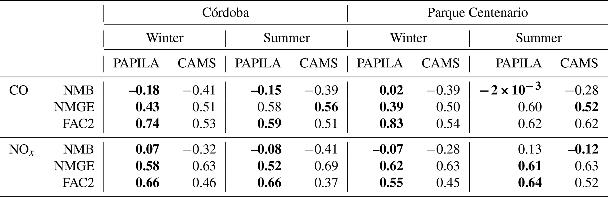
NMB: normalized mean bias; NMGE: normalized mean gross error; FAC2: fraction of predictions within a factor of 2.
Figure 5 shows the median and percentiles for CO and NOx hourly concentrations. The site Parque Centenario (residential) was better reproduced by the model with both inventories compared to Córdoba (commercial area with high traffic flow), especially in winter where the traffic flow in the city has a greater influence on the dynamics of these pollutants. However, we must also highlight that the Córdoba monitoring station is located in a corner with high traffic flow, and the sampling is at 2 m high. Therefore, the measurements may be capturing an overestimation of the real average activity in the area.

Figure 5Boxplots of hourly CO and NOx at both sites for summer and winter simulations. The dots represent the average value, the thick lines represent the medians for each period, the vertical hinges represent data points between the 25th and 75th percentiles, and the whiskers represent data points between the 5th and 95th percentiles. CO concentrations are in parts per million and NOx in parts per billion.
Scatter plots of daily mean concentrations using the PAPILA inventory (Fig. 6) depicted a good agreement between observations and model results, in winter more than in summer for CO and the other way around for NOx. Concentrations estimated with the CAMS inventory tend to be underestimated in all cases.
All in all these results show a better agreement between observations and simulations using PAPILA than CAMS to represent surface concentrations of CO and NOx in Buenos Aires. However, these emission improvements do not fully explain the underestimations of the model, especially for CO concentrations with respect to measured data.
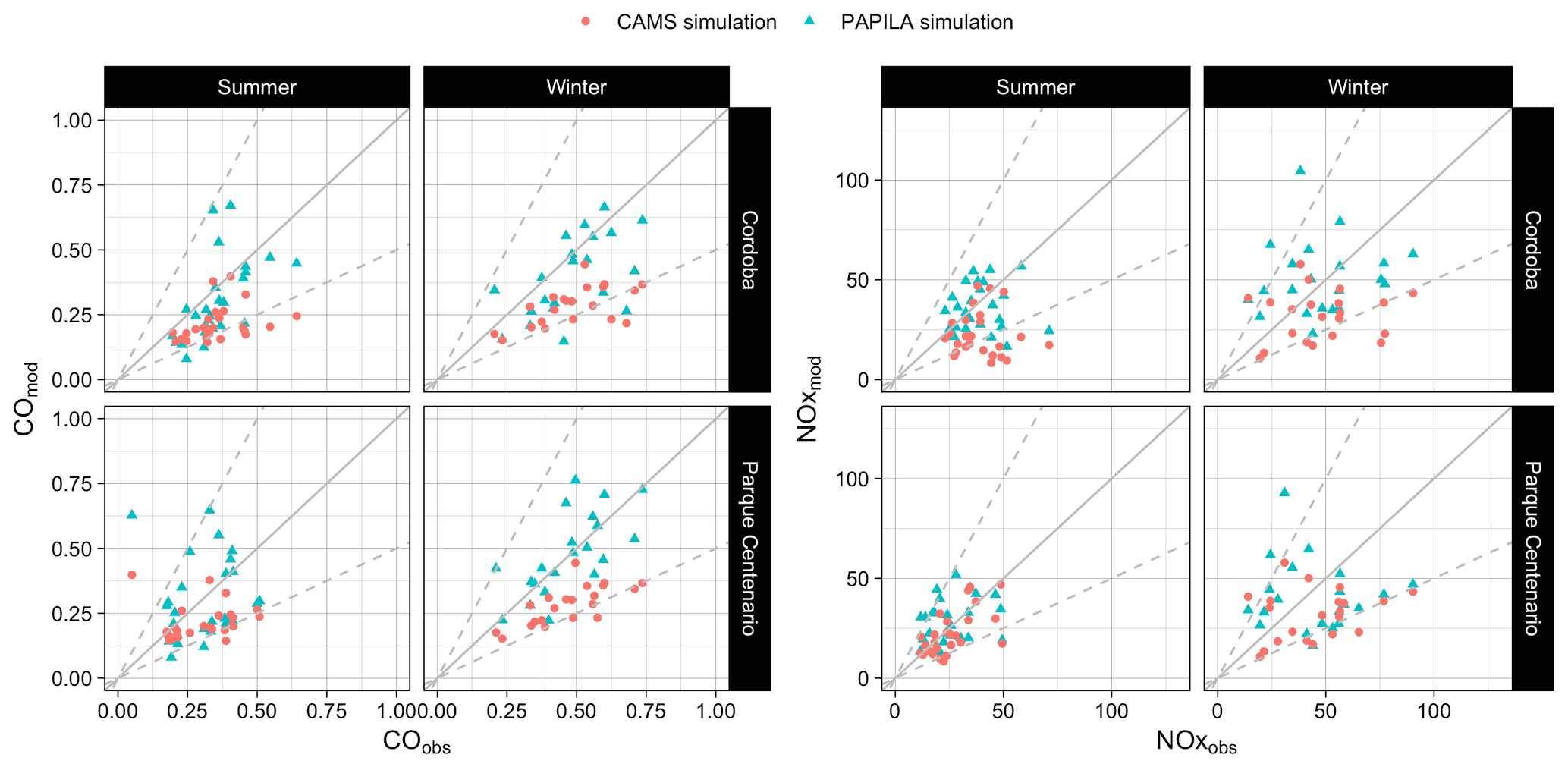
Figure 6Scatter plots for observed and modeled daily concentrations for both sites. Values within the dotted lines represent the fraction of values that are within a factor of 2 of the observations (FAC2). CO concentrations are in parts per million and NOx in parts per billion.
3.3 PAPILA–CAMS main differences
Our results show relevant differences between the PAPILA and CAMS datasets, in terms of both emission levels and their spatial distribution. They also served to exemplify the quality of the PAPILA-based simulated surface mixing ratios in the city where concentrations were analyzed.
The reasons behind the observed differences are diverse and are mainly linked to the activity data and to the methodologies applied to estimate and spatially distribute the emissions. Given the limited availability of local data, the emission factors for the compounds covered in this work were mostly based on default values in both the global and local datasets considered. In general, it is observed that CAMS-GLOB-ANT v4.1 applies linear trends to the emissions of the aggregated categories, based on the global estimates of EDGAR v4.3.2 for the year 2012. In contrast, in our work three different situations can be identified: (1) for Colombia, locally estimated trends were applied based on 2014 local emission estimates, (2) for some categories in Argentina annual estimates for the entire period were applied, and (3) for the remaining categories in Argentina and for the Chilean inventory the same methodology as used by CAMS was applied, but based on local estimates for 2014. In this way, not only are local inventories based on region-specific information, but also the extrapolation of a shorter time period reduces the uncertainties associated with the activity data strongly linked to short-term variations and technological changes.
For those activities related to fuel consumption, local inventories used the information reported in the national energy balance and other national energy statistics while global inventories are based on the information reported by the countries to the International Energy Agency (IEA), which is consistent but not exactly the same as that reported in the national statistics since the IEA processes the information received (IEA, 2020). Moreover, although these statistics adequately represent the national energy balances, it is worth pointing out the lack of specificity in terms of spatial disaggregation. A relevant aspect of the fuel consumption patterns for power generation in the three countries analyzed is their inter-annual and inter-regional variation, which in turn are strongly correlated with the water availability for hydropower generation, not captured by the extrapolations. In addition, in order for electricity supply to match demand, some short-term technological changes are often used. For example, the incorporation of diesel-fueled generators located in different urban centers in Argentina such as Buenos Aires in 2014 (CAMESA, 2021). Although the diesel consumed in these generators was reflected in international statistics, they did not distinguish between the gas oil used for this purpose and that used by combined gas cycles and could not reflect their location and operating regimes.
Another relevant aspect of national and therefore international statistics is the lack of reliable information on firewood consumption, widely used in rural areas of SA and even in some urban areas, such as the cold regions of Chile. This fact also impacts the correct representation of the replacement of firewood by LPG or natural gas that has taken place in Argentina in the last decade, due to higher production of non-conventional shale gas in the Vaca Muerta basin (El Pais, 2015) and the resulting reduction in fossil fuel prices. Additional differences between local and global datasets are related to different resolutions of the population distribution maps used as proxies for the spatial distribution of the emissions from some categories. Local inventories use population density information based on higher-resolution maps than those used by the global ones. This is clearly noticeable not only in the local–global differences found by downscaling urban domains, but also in the spatial coverage of RES emissions in global inventories, where emissions are assigned even to large non-populated areas, such as the Amazon rainforest or some desert areas of the region (Fig. 4). It is also worth mentioning that, unlike local inventories, CAMS treats countries uniformly without correcting for climatic zones, which vary widely within many of the SA countries. Broader discussions on emissions from RES are given by Puliafito et al. (2021) and Álamos et al. (2021) for Argentina and Chile, respectively.
For non-combustion sources, such as many industrial processes, population estimates are used as drivers for the CAMS projections (based on CEDS trends) (Hoesly et al., 2018). This approach may not be the most appropriate for many countries in the region, where changes in economic policies and even the occurrence of economic crises are frequent, affecting not only consumption patterns but also the relocation of activities dependent on regional economies. In addition, substantial differences have been observed in terms of the location of the IND sources in both inventories, probably attributable to the drivers used by the global databases for this purpose, with a very low presence of sources throughout the Argentine territory in CAMS and a striking abundance of sources distributed over the central and northern region in Chile, which however do not reflect the heterogeneous share of emissions shown by the local distribution.
Although the representativeness of agricultural emissions in global databases continues to improve over time, there are many aspects that global methodologies have so far failed to replicate. In this sense, the incorporation of local information has given the inventories a greater capacity to reflect the specific agricultural practices of the region, such as the predominant use of grazing for cattle farming, the use of large proportions of urea for the fertilization of crops, and economic, natural, and technological changes that have occurred during the last decades (Castesana et al., 2018, 2020).
Lastly, and with the aim of contributing some aspects that may improve both global inventories and the dataset presented here, we list some information gaps identified when using CAMS-GLOB-ANT v4.1 as a base inventory for the region: (i) emissions from domestic and international civil aviation are not included; (ii) navigation activities are not reflected by downscaling the port city B. Blanca in Argentina; (iii) CAMS assigns zero FEF emissions for species other than NMVOCs in all the downscaled urban domains; (iv) in the whole region CAMS assigns zero emissions of NMVOCs from agricultural activities, for both those from animal excreta (manure-managed AGL and deposited-in-pasture AGS) and those from crop production (AGS); and (v) CAMS assigns zero emissions of CO, NOx, and SO2 from SWD for all of SA, except for Brazil and the Guianas. Item (iii) may be attributed to the spatial distribution of FEF emissions in the global inventory, but given that this pattern is repeated in the six analyzed domains and in most of the urban domains considered there exist industrial facilities that may use venting and flaring to dispose their waste gases, the assumption of zero emissions for species other than NMVOCs seems to be more related to the omission of venting and flaring as emission sources under FEF (Granier et al., 2019). For its part, the item (v) brings to light the problems around waste management in the region, and consequently around the representativeness of the associated emissions. In SA, waste is often disposed of in open dumpsites, and, particularly regarding CO, NOx, and SO2 emissions, uncontrolled open burning occurs, and these practices are not reflected in local or global emission maps (UNEP, 2018). All these gaps in the base inventory were addressed in the PAPILA dataset, except FEF emissions and NMVOC emissions from agricultural activities in Argentina.
Gridded maps with all inventories per species and year are available as netCDF4 (Network Common Data Format) files for the regional domain (34∘ N–58∘ S, 32–120∘ W) at a resolution of 0.1∘ × 0.1∘ (PAPILA dataset) and can be accessed through the open-access data repository https://doi.org/10.17632/btf2mz4fhf.3, under a CC-BY 4 license (Castesana et al., 2021). The dataset includes all necessary attributes to be easily used in air quality simulations, such as molecular weight, projection, and units. In addition, temporal profiles applied in the inventory evaluation for the metropolitan area of Buenos Aires, Argentina, are available in Appendix A of this work.
This work presents the results of the first joint effort of South American countries to generate regional maps of emissions inventories. With a mosaic approach, we developed a new anthropogenic emission inventory for South America, named PAPILA, harmonizing inventories of Argentina, Chile, and Colombia in a uniform format. To such an end, locally developed emission inventories of these countries have been supplemented with the existing data of the global dataset CAMS-GLOB-ANT v4.1 to fill the gaps. The PAPILA dataset consists in annual emission gridded maps of reactive gases, namely CO, NOx, NMVOCs, NH3, and SO2, for the period 2014–2016 with a spatial resolution of 0.1∘ × 0.1∘ over a domain defined by 32–120∘ W and 34∘ N–58∘ S.
This study introduces significant improvements to global inventories mainly observed in the spatial distribution of emissions, in a better representation of the interannual variability of emissions strongly related with short-term variations and technological changes, and in an improvement of the representation of emissions from informal activities, such as the use of wood for heating and cooking. Relevant differences were found between both inventories at country and urban levels for all the compounds analyzed. At the national level, PAPILA presents lower CO emissions (−39 % and −54 %, respectively) for Argentina and Colombia while the opposite is observed in Chile (58 %). For NOx, PAPILA emissions for Chile and Colombia are lower than CAMS by 13 % and 7 %, respectively, whereas Argentina presents larger emissions (37 %). For NMVOCs and NH3, the only two countries with local data are Argentina and Chile. While for NMVOCs PAPILA estimates lower emissions for Argentina (−48 %) and around 3 times larger for Chile, for NH3 PAPILA estimates lower emissions in both countries, namely −7 % for Chile and −40 % for Argentina. Larger SO2 PAPILA emissions in Chile and Colombia are offset by lower emissions in Argentina (−60 %), and for the three countries together PAPILA SO2 emissions are larger by 12 %. However, CAMS emissions in these three countries represent only 31 % of the total SA emissions for SO2 and between 20 % and 25 % for the rest of the species. Therefore, further studies are necessary to complement this work with local data from other countries with significant emission levels, such as Brazil, Peru, and Venezuela.
A complete analysis of the performance of the inventory developed in this work could be provided by comparing model simulations with surface and satellite observations in the whole domain where local data have been integrated into the global dataset. Since South America is a wide region with significant differences in terms of latitudinal extension, topography, and vegetation patterns, a high-resolution model would be needed to capture the boundary layer process and surface energy budget of each area where the main changes have been introduced. As a first step of this verification exercise, we have presented a case study focused on the metropolitan area of Buenos Aires, using the WRF-Chem regional model. Although there is room for improvements that may be linked to both emissions and other processes, the CO and NOx modeling results showed a better performance with the PAPILA dataset over CAMS in reproducing surface observations in this big urban area. Nevertheless, further modeling studies with PAPILA and CAMS datasets are needed over other key areas of Argentina, Chile, and Colombia.
This work highlights the strengths and weaknesses not only of global inventories but also of local ones. Although the latter improve the representativeness of the estimates, the groups that generate information on emissions in the region do not necessarily have the same objectives: some are mainly oriented towards the generation of input information for models and others towards mitigation measures that respond to air pollution concerns of their region. In this sense, it is worth mentioning that although the resources in the region often limit their growth, the capacities of the groups are growing, which is partly reflected in the development of local databases published in this same special issue (Puliafito et al., 2021; Álamos et al., 2021; Osses et al., 2021). In addition to individual advances, we want to emphasize the role of the PAPILA project and the EMISA initiative, which promote collaboration between groups in the region, enhancing efforts aimed at the development of appropriate and consistent surface emission inventories. In this context, we trust that this work will be a starting point for the development of comprehensive emission inventories for South America enriched with local information. To this end, the first step will be to join the efforts of other countries in this endeavor, encouraging those with inventory capabilities to broaden their focus beyond cities by building national emission maps.
Table A1Description of categories and codes considered in the PAPILA inventory and their equivalence with those of CAMS.
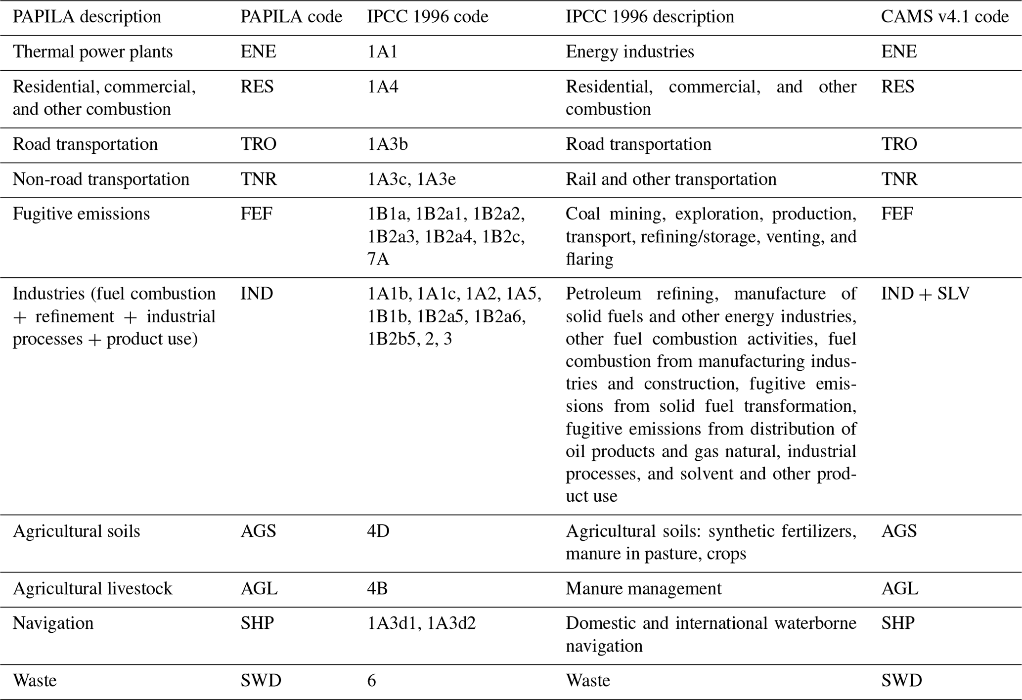
Table A2Summary of NOx and NMVOC total agricultural emissions by category for the years 2014–2016.
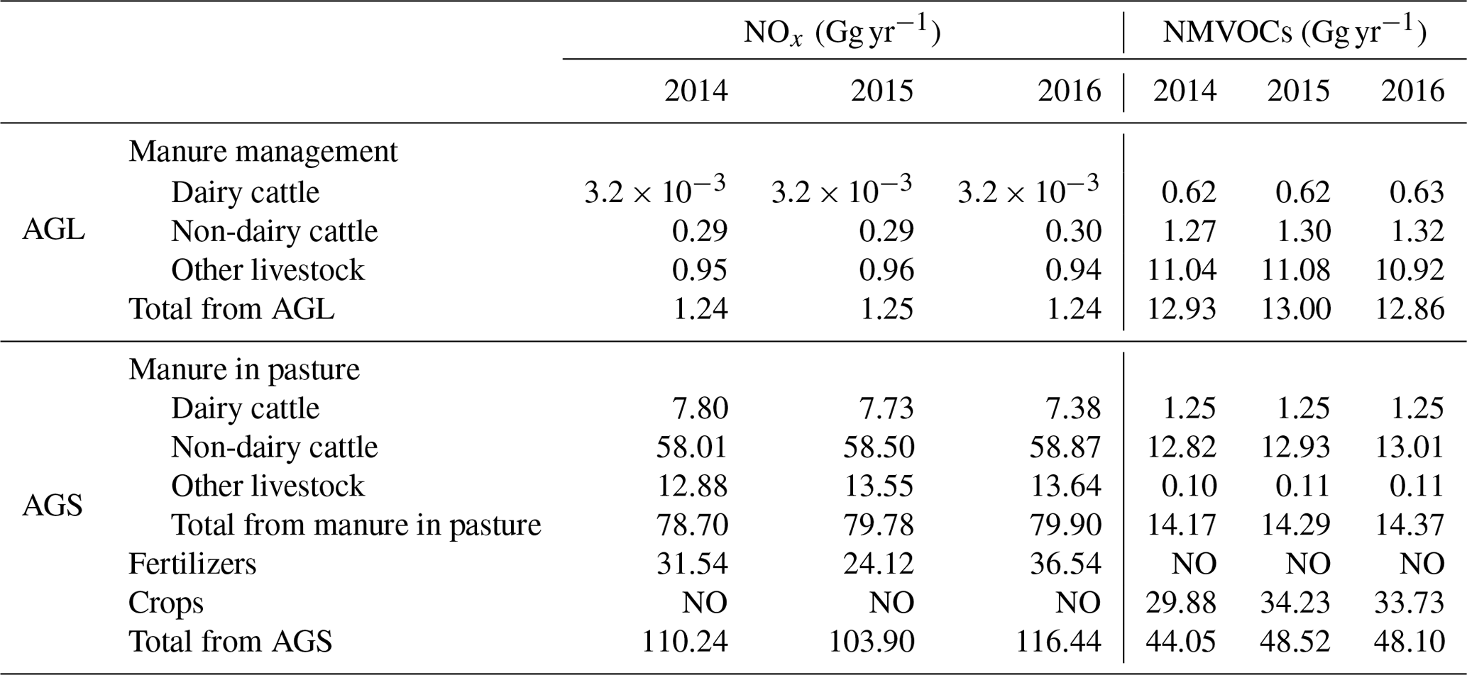
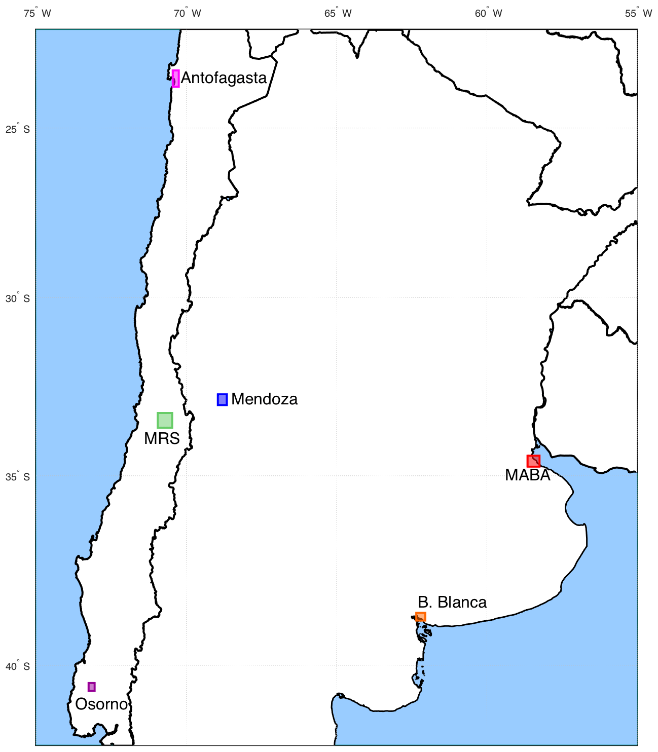
Figure A1Location of the small domains analyzed.
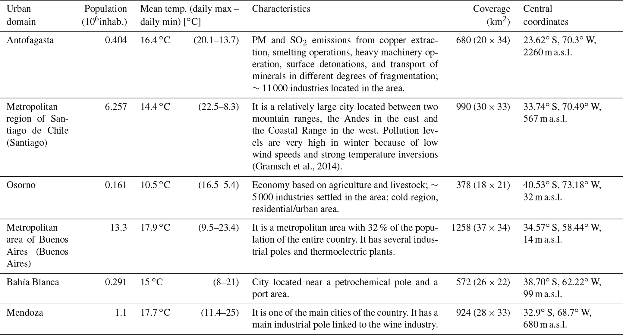
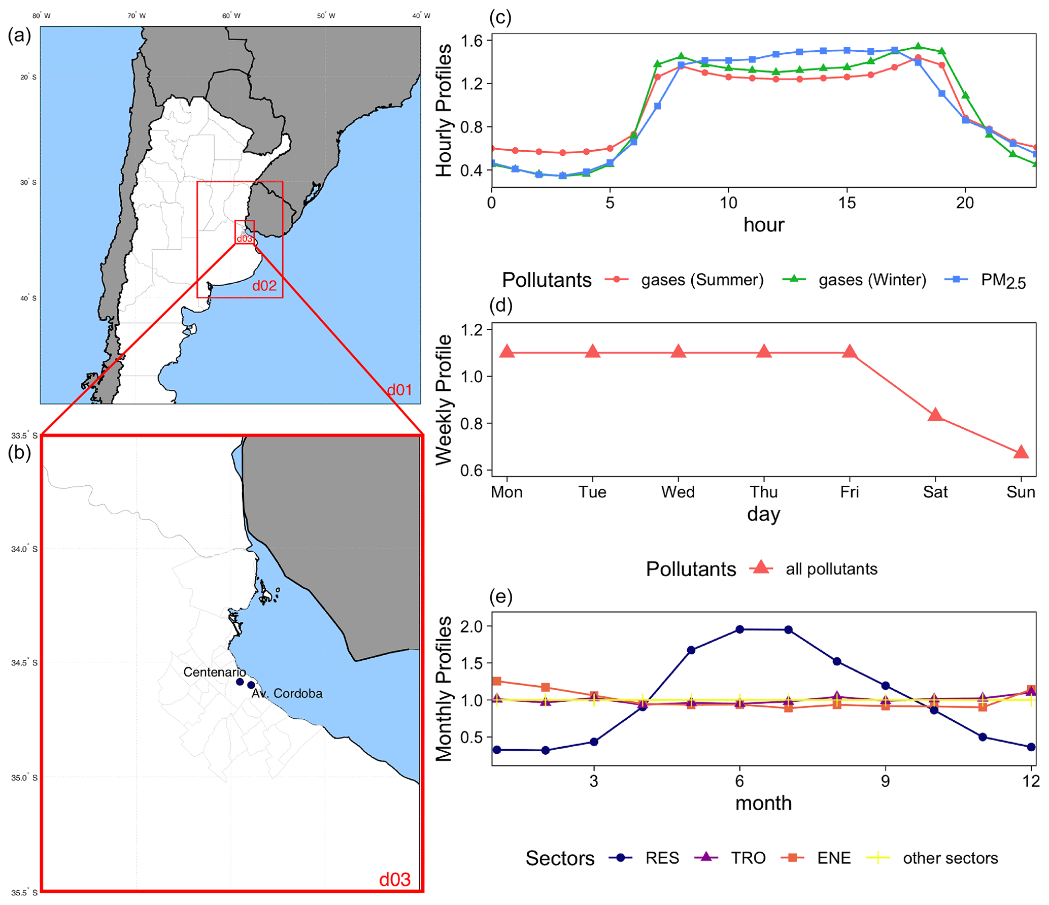
Figure A2(a, b) Location of WRF-Chem domains. Blue dots are the monitoring site locations. (c, d, e) Hourly, weekly, and monthly variations used for the temporal disaggregation of emissions within this work.
PC, MDR, CG, and LD conceived the conceptualization. PC, MDR, and LD conceived the methodology and original writing. PC, MDR, NH, EP, DG, CG, and LD helped perform the formal analysis, supervision, and writing. PC, MDR, and SD contributed to the data organization and investigation. PC, MDR, and LD coordinated the editing and prepared the manuscript with contributions from all co-authors. MOA and NR contributed to the editing.
At least one of the (co-)authors is a member of the editorial board of Earth System Science Data.
Publisher's note: Copernicus Publications remains neutral with regard to jurisdictional claims in published maps and institutional affiliations.
This article is part of the special issue “Surface emissions for atmospheric chemistry and air quality modelling”. It is not associated with a conference.
This work was conducted within the framework of the Prediction of Air Pollution in Latin America and the Caribbean (PAPILA) project. We greatly acknowledge ECCAD (https://eccad3.sedoo.fr/, last access: 22 June 2021) for the archiving and distribution of the datasets CNEA-3iA-GEIA (from Argentina), CR2-MMA (from Chile), and CAMS-GLOB-ANT v4.1 used in this work. The authors also wish to thank the Environmental Protection Agency of Buenos Aires (APRA) for sharing the air quality data for this study.
This research has been supported by the European Union H2020 program PAPILA (GA 777544), the Agencia Nacional de Promoción Científica y Tecnológica, Fondo para la Investigación Científica y Tecnológica (PICT-O 2016–4802 and PICT 2016–3590), and the Centro Científico y Tecnológico de Valparaíso (ANID PIA/APOYO AFB180002).
This paper was edited by Nellie Elguindi and reviewed by Hugo Denier van der Gon and Rafael Pedro Fernandez.
Álamos, N., Huneeus, N., Opazo, M., Osses, M., Puja, S., Pantoja, N., Denier van der Gon, H., Schueftan, A., Reyes, R., and Calvo, R.: High resolution inventory of atmospheric emissions from transport, industrial, energy, mining and residential sectors of Chile, Earth Syst. Sci. Data Discuss. [preprint], https://doi.org/10.5194/essd-2021-216, in review, 2021. a, b
Barros, V. and Camilloni, I.: La Argentina y el cambio climático, De la física a la política, EUDEBA, ISBN: 978-950-23-2655-9, 2016. a
Belincanta, J. and Alchorne, J. A., and Teixeira Da Silva, M.: The Brazilian experience with ethanol fuel: Aspects of production, use, quality and distribution logistics, Braz. J. Chem. Eng., 33, 1091–1102, https://doi.org/10.1590/0104-6632.20160334s20150088, 2016. a
CAMESA: https://portalweb.cammesa.com/default.aspx, last access: 27 June 2021. a
Castesana, P. S., Dawidowski, L. E., Finster, L., Gómez, D. R., and Taboada, M. A.: Ammonia emissions from the agriculture sector in Argentina; 2000–2012, Atmos. Environ., 178, 293–304, https://doi.org/10.1016/j.atmosenv.2018.02.003, 2018. a, b, c, d
Castesana, P. S., Vázquez-Amábile, G., Dawidowski, L. H., and Gómez, D. R.: Temporal and spatial variability of nitrous oxide emissions from agriculture in Argentina, Carbon Manag., 11, 251–263, https://doi.org/10.1080/17583004.2020.1750229, 2020. a, b
Castesana, P. S., Diaz Resquin, M. C., Huneeus, N., Puliafito, E., Darras, S., Gómez, D., Granier, C., Osses Alvarado, M., Rojas, N., and Dawidowski, L.: Data for: PAPILA dataset: a regional emission inventory of reactive gases for South America based on the combination of local and global information, v3, Mendeley Data [data set], https://doi.org/10.17632/btf2mz4fhf.3, 2021. a, b, c
CIESIN and CIAT: Gridded Population of the World, Version 3 (GPWv3): National Identifier Grid, Center for International Earth Science Information Network – CIESIN – Columbia University, and Centro Internacional de Agricultura Tropical – CIAT, NASA Socioeconomic Data and Applications Center (SEDAC) [data set], https://doi.org/10.7927/H49W0CDN, 2005. a
CR2-MMA: CR2 Emission inventory for Chile, Emissions of atmospheric Compounds and Compilation of Ancillary Data (ECCAD), [data set], available at: https://permalink.aeris-data.fr/CR2-MMA (last access: 22 June 2021), 2018. a
Dawidowski, L., Sánchez-Ccoyllo, O., and Alarcón, N.: Estimación de emisiones vehiculares en Lima Metropolitana, Informe final. Lima: SENAMHI/SAEMC, 2014. a
Dos Santos Lucon, O. and Moutinho Dos Santos, E.: The HORUS model – Inventory of atmospheric pollutant emissions from industrial combustion in Sao Paulo, Brazil, Environ. Impact Assess. Rev., 25, 197–214, https://doi.org/10.1016/j.eiar.2004.06.010, 2005. a
EDGAR: EDGAR – Emissions Database for Global Atmospheric Research, EDGAR [data set], available at: https://edgar.jrc.ec.europa.eu/emissions_data_and_maps, last access: 22 June 2021. a
El Pais: https://elpais.com/internacional/2015/06/14/actualidad/1434286413_160142.html (last access: 27 June 2021), 2015. a
EMEP: EMEP/EEA air pollutant emission inventory guidebook 2016, European Environment Agency, Copenhagen, Denmark, 2017. a
EMISA: Emission Inventories in South America, available at: https://igacproject.org/activities/emisa (last access: 7 June 2021), 2020. a
ENARGAS: Ente Nacional Regulador del Gas. Datos Abiertos: Datos operativos de Transporte y Distribución de Gas, available at: https://www.enargas.gob.ar/secciones/datos-abiertos/datos-abiertos.php, last access: 24 June 2021. a
Fioletov, V. E., McLinden, C. A., Krotkov, N., Li, C., Joiner, J., Theys, N., Carn, S., and Moran, M. D.: A global catalogue of large SO2 sources and emissions derived from the Ozone Monitoring Instrument, Atmos. Chem. Phys., 16, 11497–11519, https://doi.org/10.5194/acp-16-11497-2016, 2016. a
Freitas, S. R., Longo, K. M., Alonso, M. F., Pirre, M., Marecal, V., Grell, G., Stockler, R., Mello, R. F., and Sánchez Gácita, M.: PREP-CHEM-SRC – 1.0: a preprocessor of trace gas and aerosol emission fields for regional and global atmospheric chemistry models, Geosci. Model Dev., 4, 419–433, https://doi.org/10.5194/gmd-4-419-2011, 2011. a
Gallardo, L., Barraza, F., Ceballos, A., Galleguillos, M., Huneeus, N., Lambert, F., Ibarra, C., Munizaga, M., O'Ryan, R., Osses, M., Tolvett, S., Urquiza, A., and Véliz, K. D.: Evolution of air quality in Santiago: The role of mobility and lessons from the science-policy interface, Elementa, 6, 38, https://doi.org/10.1525/elementa.293, 2018. a, b
González-Rojas, C. H., Leiva-Guzmán, M., Manzano, C. A., Morales, R. G., and Araya, R. T.: Short-term air pollution events in the Atacama desert, Chile, J. Soc. Am. Earth Sci., 105, 103010, https://doi.org/10.1016/j.jsames.2020.103010, 2021. a
Gramsch, E., Cáceres, D., Oyola, P., Reyes, F., Vásquez, Y., Rubio, M., and Sánchez, G.: Influence of surface and subsidence thermal inversion on PM2.5 and black carbon concentration, Atmos. Environ., 98, 290–298, https://doi.org/10.1016/j.atmosenv.2014.08.066, 2014. a
Granier, C., Darras, S., Denier Van Der Gon, H., Jana, D., Elguindi, N., Bo, G., Michael, G., Marc, G., Jalkanen, J.-P., and Kuenen, J.: The Copernicus Atmosphere Monitoring Service global and regional emissions (April 2019 version), Copernicus Atmosphere Monitoring Service, 1–55, https://doi.org/10.24380/d0bn-kx16, 2019. a, b, c
Grell, G. A., Peckham, S. E., Schmitz, R., McKeen, S. A., Frost, G., Skamarock, W. C., and Eder, B.: Fully coupled “online” chemistry within the WRF model, Atmos. Environ., 39, 6957–6975, https://doi.org/10.1016/j.atmosenv.2005.04.027, 2005. a, b
Guenther, A., Karl, T., Harley, P., Wiedinmyer, C., Palmer, P. I., and Geron, C.: Estimates of global terrestrial isoprene emissions using MEGAN (Model of Emissions of Gases and Aerosols from Nature), Atmos. Chem. Phys., 6, 3181–3210, https://doi.org/10.5194/acp-6-3181-2006, 2006. a
Hoesly, R. M., Smith, S. J., Feng, L., Klimont, Z., Janssens-Maenhout, G., Pitkanen, T., Seibert, J. J., Vu, L., Andres, R. J., Bolt, R. M., Bond, T. C., Dawidowski, L., Kholod, N., Kurokawa, J.-I., Li, M., Liu, L., Lu, Z., Moura, M. C. P., O'Rourke, P. R., and Zhang, Q.: Historical (1750–2014) anthropogenic emissions of reactive gases and aerosols from the Community Emissions Data System (CEDS), Geosci. Model Dev., 11, 369–408, https://doi.org/10.5194/gmd-11-369-2018, 2018. a, b, c
Huneeus, N., Granier, C., Dawidowski, L., van der Gon, H. D., Alonso, M., Castesana, P., Diaz, M., Frost, G. J., Gallardo, L., Gomez, D., Hoesly, R., Melamed, M., Osses, M., Puliafito, E., Rojas, N., Sanchez, O., Smith, S., Tolvett, S., and Ynoue, R.: Anthropogenic emissions in South America for air quality and climate modelling, in: 2017 International Emission Inventory Conference Applying Science and Streamlining Processes to Improve Inventories, August 2017, Baltimore, United States, 2017. a
Huneeus, N., Denier van der Gon, H., Castesana, P., Menares, C., Granier, C., Granier, L., Alonso, M., de Fatima Andrade, M., Dawidowski, L., Gallardo, L., Gomez, D., Klimont, Z., Janssens-Maenhout, G., Osses, M., Puliafito, S. E., Rojas, N., Sánchez-Ccoyllo, O., Tolvett, S., and Ynoue, R. Y.: Evaluation of anthropogenic air pollutant emission inventories for South America at national and city scale, Atmos. Environ., 235, 117606, https://doi.org/10.1016/j.atmosenv.2020.117606, 2020a. a, b, c, d, e
Huneeus, N., A., U., Gayó, E., Osses, M., Arriagada, R., Valdés, M., Álamos, N., Amigo, C., Arrieta, D., Basoa, K., Billi, M., Blanco, G., Boisier, J., Calvo, R., Casielles, I., Castro, M., Chahuán, J., Christie, D., Cordero, L., Correa, V., Cortés, J., Fleming, Z., Gajardo, N., Gallardo, L., Gómez, L., Insunza, X., Iriarte, P., Labraña, J., Lambert, F., Muñoz, A., Opazo, M., O’Ryan, R., Osses, A., Plass, M., Rivas, M., Salinas, S., Santander, S., Seguel, R., Smith, P., and Tolvett, S.: Informe a las Naciones. El aire que respiramos: pasado, presente, futuro, Contaminación atmosférica por MP2,5 en el centro y sur de Chile, available at: http://www.cr2.cl/contaminacion/ (last access: 22 June 2021), 2020b. a, b
IDEAM: Prediction of Air Pollution in Latin America and the Caribbean, Institute of Hydrology, Meteorology and Environmental Studies (IDEAM), available at: http://www.cambioclimatico.gov.co/3ra-comunicacion-cambio-climatico (last access: 7 June 2021), 2017. a, b
IEA: Consistent, accurate and timely energy data and statistics, International Energy Agency, available at: https://www.iea.org/data-and-statistics (last access: 22 June 2021), 2020. a, b
Janssens-Maenhout, G., Crippa, M., Guizzardi, D., Dentener, F., Muntean, M., Pouliot, G., Keating, T., Zhang, Q., Kurokawa, J., Wankmüller, R., Denier van der Gon, H., Kuenen, J. J. P., Klimont, Z., Frost, G., Darras, S., Koffi, B., and Li, M.: HTAP_v2.2: a mosaic of regional and global emission grid maps for 2008 and 2010 to study hemispheric transport of air pollution, Atmos. Chem. Phys., 15, 11411–11432, https://doi.org/10.5194/acp-15-11411-2015, 2015. a
Janssens-Maenhout, G., Crippa, M., Guizzardi, D., Muntean, M., Schaaf, E., Dentener, F., Bergamaschi, P., Pagliari, V., Olivier, J. G. J., Peters, J. A. H. W., van Aardenne, J. A., Monni, S., Doering, U., Petrescu, A. M. R., Solazzo, E., and Oreggioni, G. D.: EDGAR v4.3.2 Global Atlas of the three major greenhouse gas emissions for the period 1970–2012, Earth Syst. Sci. Data, 11, 959–1002, https://doi.org/10.5194/essd-11-959-2019, 2019. a
Kaiser, J. W., Heil, A., Andreae, M. O., Benedetti, A., Chubarova, N., Jones, L., Morcrette, J.-J., Razinger, M., Schultz, M. G., Suttie, M., and van der Werf, G. R.: Biomass burning emissions estimated with a global fire assimilation system based on observed fire radiative power, Biogeosciences, 9, 527–554, https://doi.org/10.5194/bg-9-527-2012, 2012. a
Klimont, Z., Kupiainen, K., Heyes, C., Purohit, P., Cofala, J., Rafaj, P., Borken-Kleefeld, J., and Schöpp, W.: Global anthropogenic emissions of particulate matter including black carbon, Atmos. Chem. Phys., 17, 8681–8723, https://doi.org/10.5194/acp-17-8681-2017, 2017. a
Kuenen, J. J. P., Visschedijk, A. J. H., Jozwicka, M., and Denier van der Gon, H. A. C.: TNO-MACC_II emission inventory; a multi-year (2003–2009) consistent high-resolution European emission inventory for air quality modelling, Atmos. Chem. Phys., 14, 10963–10976, https://doi.org/10.5194/acp-14-10963-2014, 2014. a
Mazzeo, A., Huneeus, N., Ordoñez, C., Orfanoz-Cheuquelaf, A., Menut, L., Mailler, S., Valari, M., van der Gon, H. D., Gallardo, L., Muñoz, R., Donoso, R., Galleguillos, M., Osses M., and Tolvett, S.: Impact of residential combustion and transport emissions on air pollution in Santiago during winter, Atmos. Environ., 190, 195–208, 2018. a, b, c
NOAA: NCEP FNL Operational Model Global Tropospheric Analyses, continuing from July 1999, Research Data Archive at the National Center for Atmospheric Research, Computational and Information Systems Laboratory, National Centers for Environmental Prediction [data set], National Weather Service, U.S. Department of Commerce, https://doi.org/10.5065/D6M043C6, 2000. a
Ortegon-Sanchez, A. and Oviedo Hernandez, D.: Assessment of the potential for modal shift to non-motorised transport in a developing context: Case of Lima, Peru, Res. Transp. Econ., 60, 3–13, https://doi.org/10.1016/j.retrec.2016.05.010, 2016. a
Osses, M., Rojas, N., Ibarra, C., Valdebenito, V., Laengle, I., Pantoja, N., Osses, D., Basoa, K., Tolvett, S., Huneeus, N., Gallardo, L., and Gómez, B.: High-definition spatial distribution maps of on-road transport exhaust emissions in Chile, 1990–2020, Earth Syst. Sci. Data Discuss. [preprint], https://doi.org/10.5194/essd-2021-218, in review, 2021. a
PAPILA: Prediction of Air Pollution in Latin America and the Caribbean, available at: http://papila-h2020.eu/papila (last access: 7 June 2021), 2020. a
Policarpo, N. A., Silva, C., Lopes, T. F. A., Araújo, R. D. S., Cavalcante, F. S. Á., Pitombo, C. S., and de Oliveira, M. L. M.: Road vehicle emission inventory of a Brazilian metropolitan area and insights for other emerging economies, Transp. Res. D, 58, 172–185, https://doi.org/10.1016/j.trd.2017.12.004, 2018. a
Ports: Estadísticas de carga, Puertos, Vías Navegables y Marina Mercante, Ministerio de Transporte, available at: https://www.argentina.gob.ar/puertos-vias-navegables-y-marina-mercante/estadisticas-de-carga, last access: 22 June 2021. a
Puliafito, S. E., Allende, D. G., Castesana, P. S., and Ruggeri, M. F.: High-resolution atmospheric emission inventory of the argentine energy sector. Comparison with edgar global emission database, Heliyon, 3, e00489, https://doi.org/10.1016/j.heliyon.2017.e00489, 2017. a, b, c
Puliafito, S. E., Bolaño-Ortiz, T. R., Fernandez, R. P., Berná, L. L., Pascual-Flores, R. M., Urquiza, J., López-Noreña, A. I., and Tames, M. F.: High-resolution seasonal and decadal inventory of anthropogenic gas-phase and particle emissions for Argentina, Earth Syst. Sci. Data, 13, 5027–5069, https://doi.org/10.5194/essd-13-5027-2021, 2021. a, b
Romero, Y., Chicchon, N., Duarte, F., Noel, J., Ratti, C., and Nyhan, M.: Quantifying and spatial disaggregation of air pollution emissions from ground transportation in a developing country context: Case study for the Lima Metropolitan Area in Peru, Sci. Total Environ., 698, 134313, https://doi.org/10.1016/j.scitotenv.2019.134313, 2020. a, b
Secretaría de Energía: Datos Energía, Secretaría de Energia, Ministerio de Economía de la Nación, available at: http://datos.minem.gob.ar/, last access: 22 June 2021. a
Sharma, S., Sharma, P., and Khare, M.: Photo-chemical transport modelling of tropospheric ozone: A review, Atmos. Environ., 159, 34–54, https://doi.org/10.1016/j.atmosenv.2017.03.047, 2017. a
Stohl, A., Aamaas, B., Amann, M., Baker, L. H., Bellouin, N., Berntsen, T. K., Boucher, O., Cherian, R., Collins, W., Daskalakis, N., Dusinska, M., Eckhardt, S., Fuglestvedt, J. S., Harju, M., Heyes, C., Hodnebrog, Ø., Hao, J., Im, U., Kanakidou, M., Klimont, Z., Kupiainen, K., Law, K. S., Lund, M. T., Maas, R., MacIntosh, C. R., Myhre, G., Myriokefalitakis, S., Olivié, D., Quaas, J., Quennehen, B., Raut, J.-C., Rumbold, S. T., Samset, B. H., Schulz, M., Seland, Ø., Shine, K. P., Skeie, R. B., Wang, S., Yttri, K. E., and Zhu, T.: Evaluating the climate and air quality impacts of short-lived pollutants, Atmos. Chem. Phys., 15, 10529–10566, https://doi.org/10.5194/acp-15-10529-2015, 2015. a
TCN: Tercera Comunicación Nacional de la República Argentina a la Convención Marco de la Naciones Unidas para el cambio Climático, Tech. rep., Secretaría de Ambiente y Desarrollo Sustentable de la Nación, available at: https://www.argentina.gob.ar/ambiente/cambio-climatico/tercera-comunicacion (last access: 22 June 2021), 2015. a
The World Bank: Gini Index (World Bank estimate), available at: https://data.worldbank.org/indicator/SI.POV.GINI (last access: 22 June 2021), 2019. a
The World Bank: Agricultural land (% of land area), available at: https://data.worldbank.org/indicator/AG.LND.AGRI.ZS (last access: 22 June 2021), 2020. a
Thompson, G., Field, P. R., Rasmussen, R. M., and Hall, W. D.: Explicit Forecasts of Winter Precipitation Using an Improved Bulk Microphysics Scheme. Part II: Implementation of a New Snow Parameterization, Mon. Weather Rev., 136, 5095–5115, https://doi.org/10.1175/2008MWR2387.1, 2008. a
Trombetti, M., Thunis, P., Bessagnet, B., Clappier, A., Couvidat, F., Guevara, M., Kuenen, J., and López-Aparicio, S.: Spatial inter-comparison of Top-down emission inventories in European urban areas, Atmos. Environ., 173, 142–156, https://doi.org/10.1016/j.atmosenv.2017.10.032, 2018. a
UNEP: Waste Management Outlook for Latin America and the Caribbean, Programa de las Naciones Unidas para el Medio Ambiente, Oficina para América Latina y el Caribe, Ciudad de Panamá, available at: https://wedocs.unep.org/20.500.11822/26448 (last access: 22 June 2021), 2018. a
United Nations: World Urbanization Prospects The 2014 Revision, United Nations, Department of Economic and Social Affairs, Population Division, (ST/ESA/SER.A/366), 2015. a
van der Werf, G. R., Randerson, J. T., Giglio, L., Collatz, G. J., Mu, M., Kasibhatla, P. S., Morton, D. C., DeFries, R. S., Jin, Y., and van Leeuwen, T. T.: Global fire emissions and the contribution of deforestation, savanna, forest, agricultural, and peat fires (1997–2009), Atmos. Chem. Phys., 10, 11707–11735, https://doi.org/10.5194/acp-10-11707-2010, 2010. a
Villalobos, A. M., Barraza, F., Jorquera, H., and Schauer, J. J.: Wood burning pollution in southern Chile: PM2.5 source apportionment using CMB and molecular markers, Environ. Pollut., 225, 514–523, https://doi.org/10.1016/j.envpol.2017.02.069, 2017. a
Vivanco, M. G. and Andrade, M. D. F.: Validation of the emission inventory in the Sao Paulo Metropolitan Area of Brazil, based on ambient concentrations ratios of CO, NMOG and NOx and on a photochemical model, Atmos. Environ., 40, 1189–1198, https://doi.org/10.1016/j.atmosenv.2005.10.041, 2006. a
Wang, K., Zhang, Y., and Yahya, K.: Decadal application of WRF/Chem over the continental U.S.: Simulation design, sensitivity simulations, and climatological model evaluation, Atmos. Environ., 253, 118331, https://doi.org/10.1016/j.atmosenv.2021.118331, 2021. a
Wang, X., Liang, X. Z., Jiang, W., Tao, Z., Wang, J. X., Liu, H., Han, Z., Liu, S., Zhang, Y., Grell, G. A., and Peckham, S. E.: WRF-Chem simulation of East Asian air quality: Sensitivity to temporal and vertical emissions distributions, Atmos. Environ., 44, 660–669, https://doi.org/10.1016/j.atmosenv.2009.11.011, 2010. a
Wiedinmyer, C., Akagi, S. K., Yokelson, R. J., Emmons, L. K., Al-Saadi, J. A., Orlando, J. J., and Soja, A. J.: The Fire INventory from NCAR (FINN): a high resolution global model to estimate the emissions from open burning, Geosci. Model Dev., 4, 625–641, https://doi.org/10.5194/gmd-4-625-2011, 2011. a, b