High-resolution biogenic global emission inventory for the time period 2000–2019 for air quality modelling

Biogenic volatile organic compounds (BVOCs) emitted from the terrestrial vegetation into the Earth's atmosphere play an important role in atmospheric chemical processes. Gridded information of their temporal and spatial distribution is therefore needed for proper representation of the atmospheric composition by the air quality models. Here we present three newly developed high-resolution global emission inventories of the main BVOC species including isoprene, monoterpenes, sesquiterpenes, methanol, acetone and ethene. Monthly mean and monthly averaged daily profile emissions were calculated by the Model of Emission of Gases and Aerosols from Nature (MEGANv2.1) driven by meteorological reanalyses of the European Centre for Medium-Range Weather Forecasts for the period of 2000–2019. The dataset CAMS-GLOB-BIOv1.2 is based on ERA-Interim meteorology (0.5^∘ × 0.5^∘ horizontal spatial resolution); the datasets CAMS-GLOB-BIOv3.0 and v3.1 were calculated with ERA5 (both 0.25^∘ × 0.25^∘ horizontal spatial resolution). Furthermore, European isoprene emission potential data were updated using high-resolution land cover maps and detailed information of tree species composition and emission factors from the EMEP MSC-W model system. Updated isoprene emissions are included in the CAMS-GLOB-BIOv3.1 dataset. The effect of annually changing land cover on BVOC emissions is captured by the CAMS-GLOB-BIOv3.0 as it was calculated with land cover data provided by the Climate Change Initiative of the European Space Agency (ESA-CCI). The global total annual BVOC emissions averaged over the simulated period vary between the datasets from 424 to 591 Tg (C) yr⁻¹, with isoprene emissions from 299.1 to 440.5 Tg (isoprene) yr⁻¹. Differences between the datasets and variation in their emission estimates provide the emission uncertainty range and the main sources of uncertainty, i.e. meteorological inputs, emission potential data and land cover description. The CAMS-GLOB-BIO time series of isoprene and monoterpenes were compared to other available data. There is a general agreement in an interannual variability in the emission estimates, and the values fall within the uncertainty range. The CAMS-GLOB-BIO datasets (CAMS-GLOB-BIOv1.2, https://doi.org/10.24380/t53a-qw03, Sindelarova et al., 2021a; CAMS-GLOB-BIOv3.0, https://doi.org/10.24380/xs64-gj42, Sindelarova et al., 2021b; CAMS-GLOB-BIOv3.1, https://doi.org/10.24380/cv4p-5f79, Sindelarova et al., 2021c) are distributed from the Emissions of atmospheric Compounds and Compilation of Ancillary Data (ECCAD) system (https://eccad.aeris-data.fr/, last access: June 2021).

1 Introduction

The biogenic organic volatile compounds (BVOCs) consist of a vast group of non-methane hydrocarbons emitted from terrestrial vegetation and soils into the Earth's atmosphere (Kesselmeier and Staudt, 1999). They form about 90 % of the total atmospheric volatile organic compound (VOC) budget (Guenther et al., 1995), and due to their high reactivity, they are an important component of atmospheric chemistry (Atkinson and Arey, 2003). Through their oxidation in the atmosphere, BVOCs affect tropospheric photochemistry and composition (Houweling et al., 1998; Williams et al., 2013).

BVOC oxidation products play an important role in formation of low-level ozone and secondary organic aerosols, thus having impact on air quality and Earth's radiative budget. Their impact on tropospheric ozone levels was evaluated by a series of modelling studies on both global (e.g. Poisson et al., 2000; Pfister et al., 2008) and regional scales (e.g. Curci et al., 2009; Sartelet et al., 2012; Situ et al., 2013; Tagaris et al., 2014). The evidence of formation of secondary organic aerosols from BVOC oxidation products was observed by experimental studies (e.g. Griffin et al., 1999; Hao et al., 2011) and field studies (Lemire et al., 2002; Gelencser et al., 2007; Ehn et al., 2014) and consequently evaluated by atmospheric chemistry models (e.g. van Donkelaar et al., 2007; Simpson et al., 2007; Hodzic et al., 2010; Wu et al., 2020).

The emission of BVOCs from vegetation depends on many environmental factors such as meteorology, especially air temperature and solar radiation; type of vegetation; seasonal cycle; and atmospheric composition (Guenther et al., 1995). It therefore varies significantly in space and time. As biosphere–atmosphere interaction is a very complex system with mutual feedbacks, efforts have been made to assess the impact of different driving factors, which themselves are changing and/or are expected to change in the future. Interest has been focused mainly on impact of changing climate, land cover and atmospheric CO₂ concentration in the recent past (e.g. Naik et al., 2004; Lathière et al., 2006; Arneth et al., 2007a; Stavrakou et al., 2014) as well as in the future (e.g. Sanderson et al., 2003; Heald et al., 2008; Hantson et al., 2017).

Given the importance of BVOCs in the atmospheric composition, proper information about amount and spatio-temporal distribution of BVOC emissions is a crucial input to atmospheric chemistry and climate models. Different ground-based measurement techniques can be applied to sample BVOC emissions at different scales, from leaf to regional level, as summarized by Hewitt et al. (2011). Many measurement campaigns have been organized in the past to evaluate BVOC emission fluxes in different parts of the world, especially in the tropics, which have the highest emission potential, such as the Amazon (e.g. Rinne et al., 2002; Kuhn et al., 2007; Karl et al., 2007; Eerdekens et al., 2009) and Southeast Asia (e.g. Langford et al., 2010; Misztal et al., 2011). However, such measurements are unfortunately limited in space and time and are therefore not fully suitable to create a long-term gridded inventory of BVOC emissions required by the models. Knowledge obtained from observations on the emission processes, speciation and evaluation of fluxes serves as a valuable baseline for development of the emission BVOC models, which are then able to simulate BVOC emissions for a specific time period and spatial domain based on defined input parameters.

Over time a relatively long list of BVOC emission models have been developed. The models differ in the approach used to estimate BVOC, in the level of complexity in processes considered and in factors affecting the emission. In general, there are two main approaches to BVOC modelling: first, a so-called process-based model that simulates BVOC synthesis directly inside the plant (e.g. LPJ-GUESS, Lund–Potsdam–Jenna General Ecosystem Simulator; JULES, Joint UK Land Environment Simulator), and second, an approach based on a semi-empirical algorithm described by Guenther et al. (1995) which defines dependence of BVOC emissions from the plant on environmental factors, namely air temperature and solar radiation. The MEGAN model (Model of Emissions of Gases and Aerosols from Nature) was developed from the latter, widely used in the BVOC emission and atmospheric chemical and climate modelling communities. The emission algorithms can be either stand-alone or embedded inside an Earth system, land surface or air quality model.

Different BVOC emission models were applied in the past to obtain estimates of BVOC emission levels on a global scale (e.g. Lathière et al., 2005; Müller et al., 2008; Arneth et al., 2007b; Schurgers et al., 2009; Pacifico et al., 2011; Guenther et al., 2012; Sindelarova et al., 2014; Messina et al., 2016). Similarly, there exists a long list of studies focusing on the regional level (e.g. Simpson et al., 1995, 1999; Steinbrecher et al., 2009; Karl et al., 2009; Oderbolz et al., 2013; Emmerson et al., 2018). These inventories are so-called “bottom-up” inventories, i.e. calculated by the emission models based on surface input data.

With emerging availability of satellite-based observations of the Earth's atmosphere, data retrieved from space started to be used also in BVOC emission estimation. Spaceborne measurements of suitable chemical species are used to constrain a priori emissions through an inversion technique applied in the atmospheric chemistry model. Such an approach has been applied for example to constrain emissions of isoprene, the most abundant BVOC species, with satellite measurements of isoprene's oxidation product formaldehyde (e.g. Palmer et al., 2006; Millet et al., 2008; Stavrakou et al., 2009; Curci et al., 2010; Bauwens et al., 2016; Kaiser et al., 2018). Emission inventories constrained by satellite observations through application of the model inversion are being called “top-down”. Recently, a methodology for direct measurement of isoprene emissions from space has been developed by identifying spectral signatures of isoprene in satellite-borne measurements of the Cross-track Infrared Sounder (Fu et al., 2019; Wells et al., 2020).

In this paper we present three new global bottom-up inventories of BVOC emissions calculated with a modified version of the state-of-the-art emission model MEGANv2.1 (Guenther et al., 2012) forced by meteorological reanalyses of the European Centre for Medium-Range Weather Forecasts (ECMWF) and high-resolution input data. The inventories contain global gridded emissions of the main BVOC species for a 20-year period (2000–2019) which can be directly used as an input to the air quality and climate models.

In the following section (Sect. 2) we describe a methodology of emission calculation, including a description of the emission model and input meteorological, land cover and emission factor data. Section 3 presents global and regional distribution of emission estimates, together with comparison of emission inventories within each other and with other available data. Information on data availability is given in Sect. 4, and conclusions and a summary are presented in Sect. 5.

2 Methodology

2.1 Emission model

The presented emission datasets were calculated using the Model of Emissions of Gases and Aerosols from Nature (MEGANv2.1; Guenther et al., 2012). The MEGAN model was developed at the National Center for Atmospheric Research (NCAR, US) and is currently maintained and further improved by the Biosphere Atmosphere Interaction Group at the University of California – Irvine (https://bai.ess.uci.edu/, last access: 18 January 2022).

It is an emission model extensively used in the atmospheric modelling community for simulation of biogenic VOC emissions from vegetation and soils at regional and global scales (e.g. Guenther et al., 2006; Heald et al., 2008; Arneth et al., 2011; Sindelarova et al., 2014; Seco et al., 2015; Emmerson et al., 2018; Kaiser et al., 2018, Huszar et al., 2018, 2020). Furthermore, the algorithm of the MEGAN model has been embedded into a number of Earth system and chemical transport models (e.g. Emmons et al., 2010; Lawrence et al., 2011; Keller et al., 2014; Henrot et al., 2017).

The model calculates an emission flux F ($\mathrm{\mu }\mathrm{g}\mathrm{grid}{\mathrm{cell}}^{-\mathrm{1}}{\mathrm{h}}^{-\mathrm{1}}$) of specific BVOC species from a model grid cell as follows:

$$\begin{array}{}\text{(1)}& F=\mathit{\gamma }\cdot \text{EP}\cdot S,\end{array}$$

where γ is a dimensionless factor accounting for dependence of emissions on environmental factors (air temperature, solar radiation, ambient CO₂ concentration, leaf age, etc.); EP ($\mathrm{\mu }\mathrm{g}{\mathrm{m}}^{-\mathrm{2}}{\mathrm{h}}^{-\mathrm{1}}$) is an emission potential of a grid cell, i.e. a unit emission defined under standardized environmental conditions; and S (m²) is a grid cell surface area. The MEGANv2.1 was applied with the full canopy module, which calculates meteorological conditions inside the forest canopy (e.g. leaf temperature, radiation on sunlit and shaded leaves). For calculation of isoprene, the model took into account an inhibitory effect of CO₂ concentration on isoprene emissions using parametrization described in Heald et al. (2009). In our simulations, we did not consider the effect of soil moisture stress on the plant emissions. For more details on the MEGANv2.1 algorithm please see Guenther et al. (2006, 2012).

2.2 Meteorology

Two sources of meteorological data were used for calculation of the emission datasets. CAMS-GLOB-BIOv1.2 is based on the ERA-Interim (Dee et al., 2011) data, and the datasets CAMS-GLOB-BIOv3.0 and v3.1 were calculated with ERA5 (Hersbach et al., 2020), both meteorological reanalyses of the European Centre for Medium-Range Weather Forecasts (ECWMF). The MEGAN model requires the following input parameters: 2 m air temperature, water mixing ratio, surface pressure, 10 m wind speed and photosynthetically active radiation (PAR). PAR is defined as solar radiation with a wavelength between 400 and 700 nm, which photosynthetic organisms are able to absorb during photosynthesis. Unfortunately, this parameter is available neither in ERA-Interim nor ERA5 datasets (see Copernicus Knowledge Base – ERA-Interim: surface photosynthetically active radiation (surface PAR) values are too low, 2017). PAR was therefore approximated with surface solar downward radiation divided by a factor of 2.2 as recommended by various studies (Olofsson et al., 2007; Jacovides et al., 2003; Escobedo et al., 2011). The water mixing ratio was calculated from 2 m dew point temperature following equations from Lowe and Ficke (1974).

Since emissions are calculated on a monthly mean basis, the input meteorological data were synoptic monthly means of analysed and forecasted parameters. ERA-Interim data were available on a global grid with horizontal spatial resolution of 0.5^∘ × 0.5^∘ with 3 or 6 h time steps. The data were linearly interpolated in time in order to obtain a monthly averaged daily profile of each meteorological variable. ERA5 is a successor to ERA-Interim, with higher horizontal spatial resolution of 0.25^∘ × 0.25^∘ and with 1 h time resolution. Interpolation between time steps was therefore no longer necessary in the case of ERA5.

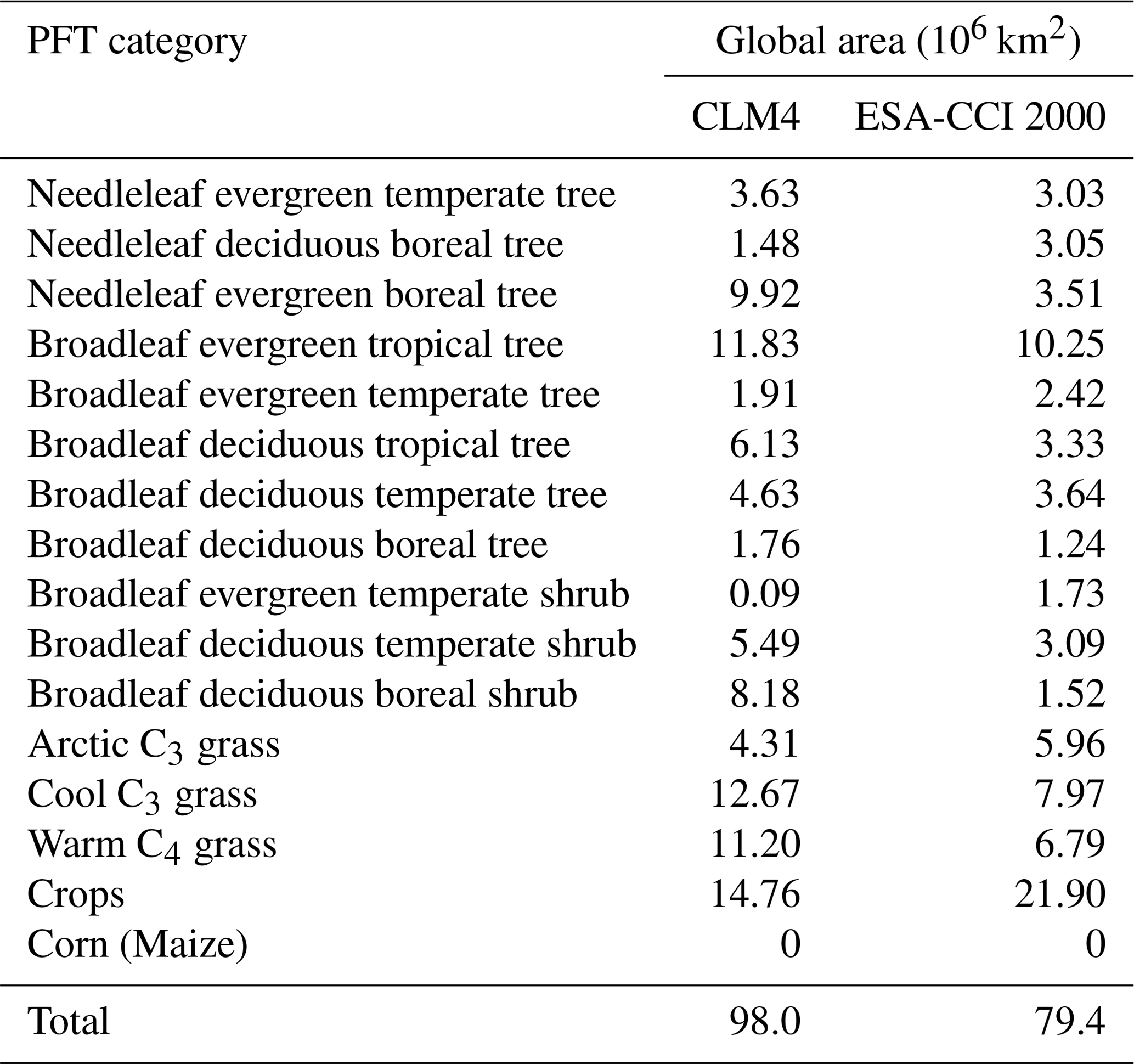
Table 1 List of MEGANv2.1 PFT categories and global coverage by each PFT category (10⁶ km²) according to CLM4 and ESA-CCI (year 2000) land cover maps.

2.3 Vegetation description

The spatial distribution of vegetation in the MEGAN model is defined using plant functional types (PFTs). This is an alternative approach to vegetation description using biomes (e.g. savanna, tundra). While biomes can consist of physiologically distinct vegetation types (e.g. grasses and trees), plant functional types group vegetation with similar leaf physiology. Use of PFTs leads to less complex vegetation representation but allows physiologically based ecosystem description convenient for the dynamic global vegetation models. The MEGAN model was designed to be coupled with the Community Land model (CLM4) and therefore uses the same approach, i.e. representation of the global land cover with 16 PFT categories (Lawrence and Chase, 2007). Vegetation in each model grid cell is defined by fractional coverage by each of the PFTs. A list of the MEGANv2.1 PFT categories is given in Table 1.

Emissions in CAMS-GLOB-BIOv1.2 and v3.1 were calculated with a temporally invariable map of PFTs from the CLM4 model representative of the year 2000. However, global land use and land cover are experiencing dramatic changes, e.g. deforestation in the tropical forests and replacement of forests by agricultural land (e.g. Song et al., 2018), which is obviously expected to impact the BVOC emissions. In order to capture the land cover change in MEGAN simulations, we replaced the static CLM4 PFT map with land cover data from the ESA-CCI (ESA, 2017). ESA-CCI data are provided by the Climate Change Initiative of the European Space Agency. The data consist of time series of global annual mean land cover maps with high horizontal spatial resolution (300 m) available for the period of 1992–2018 based on satellite observations. To be consistent with the MEGAN model, the ESA-CCI land cover categories were converted to PFT classes similar to the CLM4 using the CCI-LC user tool v4.3 (Poulter et al., 2015). Emissions calculated with temporally varying land cover are included in the CAMS-GLOB-BIOv3.0 dataset.

Table 1 compares global land areas covered by each PFT category in CLM4 and ESA-CCI (year 2000, converted by the CCI-LC user tool) land cover maps. Note that though the corn (maize) category is included in the MEGAN PFT list, it is currently not distinguished from other crops, and its spatial coverage is therefore zero. The two maps differ in the total area covered by vegetation, with ESA-CCI giving ∼ 19 % less vegetated area globally. In ESA-CCI, the extent of the tree and grass categories is ∼ 25 % lower, while coverage by the crop category is almost 50 % higher when compared to CLM4.

Vegetation seasonality is represented by changes in leaf area index (LAI). LAI is a dimensionless parameter defined as one-sided leaf area per area of the ground surface (m² m⁻²). Spatial and temporal distribution of LAI was obtained from processed observations of the MODIS instrument (Yuan et al., 2011). The 8 d observations were averaged to monthly means. The Yuan et al. (2011) LAI data are available for the period of 2000–2016. For the emissions calculated after 2016 a 10-year climatology was used. Since these LAI values represent an average over the whole grid cell, values were divided by a grid cell fraction covered by vegetation to obtain LAI for vegetated area only.

2.4 Global emission potential data

Emission potentials, together with the vegetation description, are a crucial parameter in BVOC emission estimation. In the following text we distinguish between emission factor (EF) and emission potential (EP). By EF we mean emission of a chemical species from specific plant or vegetation type under standard conditions of environmental parameters. EFs can be defined either as area-based values, i.e. an emission from a unit area covered by specific plant or vegetation type (e.g. $\mathrm{\mu }\mathrm{g}\left(\mathrm{species}\right){\mathrm{m}}^{-\mathrm{2}}\left(\mathrm{groundcover}\right){\mathrm{h}}^{-\mathrm{1}}$), or mass-based values, i.e. emission from a unit mass of the plant's dry leaf matter (e.g. $\mathrm{\mu }\mathrm{g}\left(\mathrm{species}\right){\mathrm{g}}^{-\mathrm{1}}\left(\mathrm{dry}\mathrm{foliar}\mathrm{mass}\right){\mathrm{h}}^{-\mathrm{1}}$). With emission potential ($\mathrm{\mu }\mathrm{g}{\mathrm{m}}^{-\mathrm{2}}{\mathrm{h}}^{-\mathrm{1}}$) we describe the emission capacity of the whole grid cell, which is calculated as a weighted sum of emission factors for all plants or vegetation types present in the grid cell:

$$\begin{array}{}\text{(2)}& \mathrm{\text{EP}}=\sum _{\text{veg}}{f}_i{\text{EF}}_i\left(\mathrm{\mu }\mathrm{g}{\mathrm{m}}^{-\mathrm{2}}{\mathrm{h}}^{-\mathrm{1}}\right)=\sum _{\text{veg}}{f}_i{\text{EF}}_i\left(\mathrm{\mu }\mathrm{g}{\mathrm{g}}^{-\mathrm{1}}{\mathrm{h}}^{-\mathrm{1}}\right)D_i,\end{array}$$

where f_i is a fraction of a grid cell covered by individual plant or vegetation type, and D_i (g (dry leaf matter) m⁻²) is a foliar density of the plant or vegetation type.

Emission factors in the MEGANv2.1 model are defined on a canopy-scale level as an emission under standard conditions from the full canopy. Above-canopy measurements of EF are unfortunately limited; therefore the canopy-scale EFs in MEGAN are still based on leaf- and branch-scale measurements, which were extrapolated with a canopy environment model to the canopy level (Guenther et al., 2006). MEGAN standard conditions are defined for a series of variables, such as LAI, leaf age composition of the canopy, and meteorological conditions (temperature, solar radiation, humidity, wind speed, soil moisture) of the current state and of the past (temperature and solar radiation). For more details see Guenther et al. (2006).

The MEGAN model has two options for emission potential definition: either use of the input emission potential maps for selected species or calculation of EP from vegetation coverage. These options are described in more detail in the two following sections.

2.4.1 Emission potentials from detailed global maps

The first option consists of the use of annual mean emission potential maps with high spatial resolution for the main BVOC species, i.e. isoprene, main monoterpenes (α-pinene, β-pinene, myrcene, sabinene, limonene, trans-β-ocimene, 3Δ-carene) and 2-methyl-3-buten-2-ol (MBO). Emission maps are available together with the MEGANv2.1 code (https://bai.ess.uci.edu/megan/data-and-code/megan21, last access: 31 May 2021) and were created based on detailed ecoregion description, combining information on species composition with species-specific emission factors and above-canopy flux measurements where available (Guenther et al., 2012). Emission potentials for the rest of the modelled species were calculated based on the PFT coverage as described in the following section.

Table 2 Updated emission factors for α-pinene ($\mathrm{\mu }\mathrm{g}{\mathrm{m}}^{-\mathrm{2}}{\mathrm{h}}^{-\mathrm{1}}$) for tree PFT classes used in this study based on Messina et al. (2016) together with original MEGANv2.1 EFs (Guenther et al., 2012).

2.4.2 Emission potentials calculated from PFTs

The second option consists of EP calculation from the vegetation composition of each grid cell. MEGAN uses 16 PFTs for description of vegetation in the model domain (listed in Table 1). Each of the PFTs is assigned with an emission factor value for each of the modelled species (see Table 2 in Guenther et al., 2012). The emission potential of each grid cell for a specific modelled chemical species is then calculated as a weighted sum defined in Eq. (2).

We performed specific emission model runs to evaluate the difference in resulting emissions when emissions are calculated from EP detailed maps and from EP calculated based on the PFT coverage. All the other input parameters were kept the same. Use of EP calculated from the PFT coverage leads to a ∼ 10 % decrease in isoprene emission total on a global scale when compared to emission calculation based on EP detailed maps. For β-pinene and other monoterpenes the difference is only 1 %–2 %. However, for α-pinene, emissions calculated from PFT coverage are more than 70 % higher when compared to emissions calculated from the EP maps. Therefore, the EFs assigned to each PFT tree category for α-pinene were revised based on recent updates of EFs for the ORCHIDEE model (Messina et al., 2016). The ORCHIDEE and MEGAN models differ in the definition of standard conditions, which means that the ORCHIDEE EFs needed to be converted to MEGAN-suitable format. The conversion was done in a similar way as described in Sect. 2.5.2. The newly used α-pinene EFs are listed in Table 2 together with the original MEGANv2.1 values. The resulting α-pinene emissions calculated with revised EFs are ∼ 18 % higher than emissions calculated with the detailed EP map.

Describing global vegetation by only 16 PFT categories is of course a simplification that inevitably brings inaccuracies, especially for categories such as broadleaf deciduous forest, which can consist of tree species which are very low isoprene emitters but at the same time tree species such as oaks, which are very strong isoprene emitters. On the other hand, such simplifications are often necessary due to lack of detailed information on vegetation composition and/or assignment with emission factor or are simply a result of balance between the level of detail in vegetation description and ability of the model algorithm to digest such data.

Calculation of EP from PFT coverage is to some extent inaccurate and on the other hand allows us to change the land cover description dataset (e.g. use ESA-CCI instead of CLM4) and therefore study the impact of land cover on resulting emissions.

2.5 Update of isoprene emission potentials in Europe

The MEGAN global input emission potential maps for isoprene and main monoterpenes were created based on information of global land cover distribution and vegetation composition in combination with emission factor survey, incorporating results of flux measurement campaigns. Naturally, a lot of information on emission factor and flux measurements originates in the tropics as it is a region of the highest emission rates. This leads to the fact that the MEGAN emission potential maps are well suited for the tropical region but may be less fitting in other parts of the world.

As detailed land cover data were becoming available for Europe, studies focusing on estimation of biogenic VOCs from plant-specific vegetation descriptions started to appear (e.g. Simpson et al., 1995, 1999; Karl et al., 2009; Oderbolz et al., 2013). Several studies have shown large discrepancies between emissions calculated using species-specific emission factors and those calculated by MEGAN-based inputs (Rinne et al., 2009; Langner et al., 2012; Jiang et al., 2019). This motivated us to revise the input emission potential maps for isoprene in this region.

In this work, new maps of area-based isoprene emission potentials (EPs; $\mathrm{\mu }\mathrm{g}{\mathrm{m}}^{-\mathrm{2}}{\mathrm{h}}^{-\mathrm{1}}$) for the European area were created. These EP maps are based on detailed maps of forest species and other vegetation combined with Europe-specific emission factors for each species. The EP map update makes use of procedures developed over many years for the EMEP model (Simpson et al., 1995, 1999, 2012). The basic emission factors and LAI changes are taken from a high-resolution version of the EMEP model rv4.33 (Simpson et al., 2012).

The EMEP and MEGANv2.1 models differ in their definition of standard environmental conditions for emission factors. In MEGANv2.1 EFs are defined on the canopy-scale level, i.e. as an emission from the full canopy, under standardized canopy conditions of LAI, specific proportion of mature, growing and old foliage, current and previous air temperatures and radiation, humidity, wind speed, and soil moisture (Guenther et al., 2006, 2012). The EMEP system, similar to previous BVOC algorithms of Guenther et al. (1995), uses a leaf- and branch-level EF definition with standard conditions for leaf temperature (30 ^∘C) and photosynthetically active radiation (1000 $\mathrm{\mu }\mathrm{mol}{\mathrm{m}}^{-\mathrm{2}}{\mathrm{s}}^{-\mathrm{1}}$) only. As canopy-scale EFs are not available for the vegetation species used for this isoprene EP update, a new map was created with leaf- and branch-level EFs. The new isoprene EP values were then converted to MEGANv2.1-suitable format. There is unfortunately no accurate conversion equation that would satisfy all conditions. A rough conversion can be made following recommendations by Arneth et al. (2011) and Messina et al. (2016) for conversion between the two systems. Details of the conversion of EMEP EFs to MEGANv2.1-suitable isoprene EPs are given in Sect. 2.5.2.

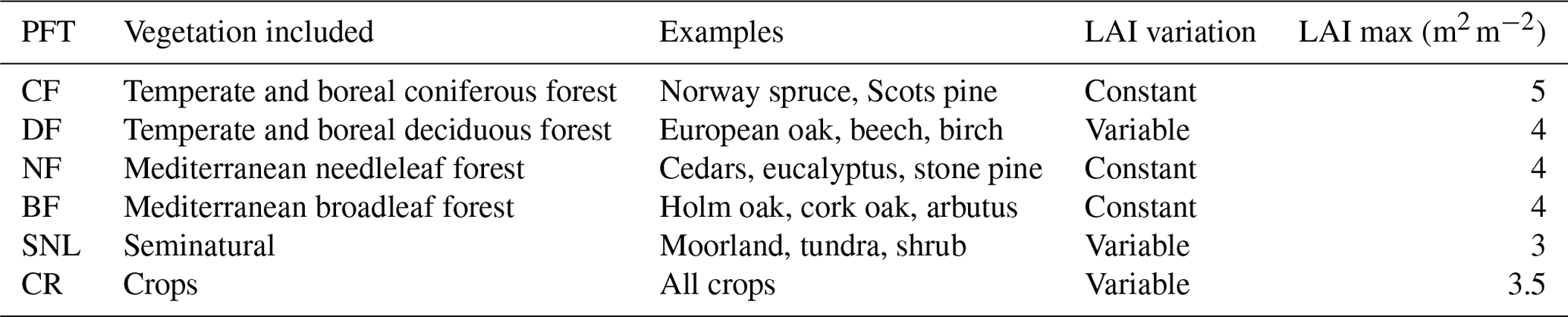
Table 3 Generic PFTs used for European emission potential maps based on EMEP.

2.5.1 Land cover description and emission factors

The main basis for European BVOC emissions in Europe in the EMEP system is a map of forest species generated by Köble and Seufert (2001), combined with species-specific EFs for each of these species. The forest database provides maps for 115 tree species in 30 (mainly EU) European countries based on a compilation of data from the ICP-forest network (UN-ECE, 1998). These data were further processed to the EMEP grid by the Stockholm Environment Institute at York (UK, Steven Cinderby, personal communication, 2004) in order to add data from other countries in the (2000 era) EMEP domain and for non-forested vegetation. More recently, the EMEP domain was significantly expanded to the east, and data for the expanded area and indeed globally make use of a merger of the GLC_2000 dataset (https://forobs.jrc.ec.europa.eu/products/glc2000/products.php, last access: 18 January 2022) and data from the Community Land Model (https://www.cesm.ucar.edu/models/clm/, last access: 18 January 2022; Oleson et al., 2010; Lawrence et al., 2011) as described in Simpson et al. (2017). In order to provide a manageable number of PFTs for use in MEGAN, tree species were aggregated in six classes, as summarized in Table 3.

For each grid cell, the grid-average emission potential of a specific PFT (EP_PFT; $\mathrm{\mu }\mathrm{g}{\mathrm{m}}^{-\mathrm{2}}{\mathrm{h}}^{-\mathrm{1}}$) was then calculated as a weighted average of all the individual tree species belonging to this PFT category:

$$\begin{array}{}\text{(3)}& {\text{EP}}_{\text{PFT}}={\displaystyle \frac{{\sum }_i{\text{EF}}_i{D}_i{A}_i}{{\sum }_i{A}_i}},\end{array}$$

where i represents one of the many forest or vegetation species contained within that PFT, EF_i is the species foliage-level isoprene emission factor ($\mathrm{\mu }\mathrm{g}\mathrm{g}(\mathrm{dry}\mathrm{leaf}\mathrm{weight}{)}^{-\mathrm{1}}{\mathrm{h}}^{-\mathrm{1}}$), D_i is the species foliar density (g (dry leaf weight) m⁻²), and A_i is the species area (m²). Further details of this methodology, including detailed composition of each PFT class as well as EF and D values for each considered tree species, can be found in Simpson et al. (2012) (Sect. 6.6., Supplement, Sect. S4.4 therein).

For the European-domain runs used here, the EMEP model combines the PFT-specific EPs and max LAI with latitude-dependent growing season dates as described in Simpson et al. (2012). For this work we have made use of much finer grid resolution (0.1^∘ × 0.1^∘ latitude–longitude).

For non-forest vegetation types (e.g. grasslands, seminatural vegetation) or for forest areas not covered by the Köble and Seufert (2001) maps (e.g. for eastern Russia), default emission factors taken from Simpson et al. (2012) were applied.

The crop category is the most difficult to deal with in terms of BVOC emissions, not least because the types of crops are not well known (and can change significantly over the years), and the growing seasons are almost impossible to specify. Here we used a simple system which defines the phenology and emission factors of crops using EMEP model definitions. For this study, the EMEP model's temperate crop (e.g. wheat), Mediterranean crop (e.g. maize) and root crop (e.g. potato) were aggregated into one crop PFT.

The isoprene emission potential data (EF_PFT) and the monthly changes in LAI per each of the six PFTs were provided for a European domain spanning (30.05–71.95^∘) in latitude and (−29.95–65.95^∘) in longitude with 0.1^∘ × 0.1^∘ spatial resolution.

2.5.2 Conversion of isoprene emission potential map for MEGAN

In order to satisfy the MEGANv2.1 definition of standard conditions, the EMEP-based isoprene emission potential maps needed to be converted. As discussed earlier, there is unfortunately no precise way of such conversion. According to recommendations of Arneth et al. (2011) and Messina et al. (2016), the following equation was used for conversion between the EMEP and MEGANv2.1 system.

MEGAN-suitable isoprene emission potentials EP_MEGAN ($\mathrm{\mu }\mathrm{g}{\mathrm{m}}^{-\mathrm{2}}{\mathrm{h}}^{-\mathrm{1}}$) were calculated for each month as

$$\begin{array}{}\text{(4)}& {\text{EP}}_{\text{MEGAN}}\left[\text{month}\right]={\text{LAI}}_{\text{std}}{\displaystyle \frac{{\sum }_i^{\text{PFT}}{f}_i\frac{{\text{LAI}}_i\left[\text{month}\right]}{{\text{LAI}}_{max}}{\text{EP}}_{\text{PFT}i}}{{\sum }_i^{\text{PFT}}{f}_i{\text{LAI}}_i\left[\text{month}\right]}},\end{array}$$

where LAI_std is standard leaf area index in the MEGAN model equal to 5 m² m⁻²; i is an index through EMEP PFT categories (Table 3); f is a fraction of a grid cell covered by a specific PFT; LAI and LAI_max are monthly and maximal leaf area index of the PFT category (see Table 3), respectively; and EP_PFT is EMEP-based isoprene emission potential for a specific PFT category.

Monthly isoprene emission potential maps for Europe were then embedded into the global domain of MEGAN gridded emission potential maps. These new global isoprene EPs were used in the calculation of the CAMS-GLOB-BIOv3.1 emission inventory.

Table 4 Summary of CAMS-GLOB-BIO inventories. Description of horizontal spatial resolution, meteorology driving each dataset, land cover description and emission potential (EP) data used in each inventory.

3 Results and discussion

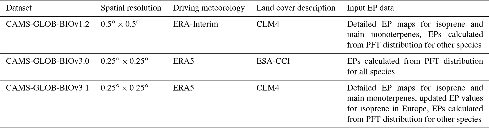
The following sections present examples of spatial and temporal distribution of emissions in CAMS-GLOB-BIO inventories on global and regional scales (Sect. 3.1 and 3.2). Section 3.3 focuses in more detail on the impact of land cover change on isoprene emissions, and Sect. 3.4 focuses on updates of the isoprene emission potential data in Europe, showing differences between emissions calculated with the MEGAN default and updated input EP maps. Section 3.5 presents a comparison of CAMS-GLOB-BIO isoprene and monoterpene emissions to other available datasets. Table 4 summarizes the data availability in each CAMS-GLOB-BIO inventory as well as the different input parameters used to calculate each dataset.

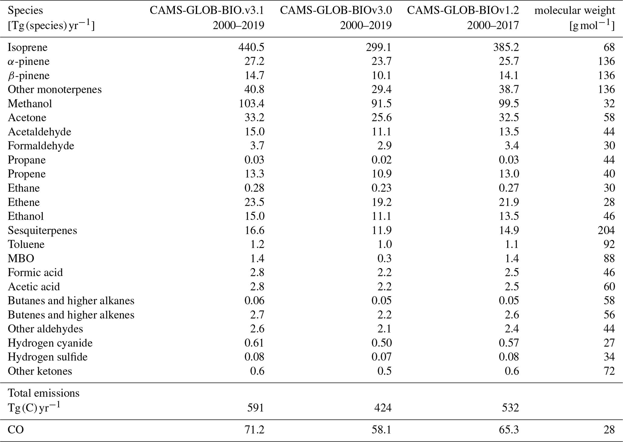
Table 5 List of modelled BVOC species with annual global emission totals (Tg (species) yr⁻¹) in CAMS-GLOB-BIOv3.1, v3.0 and v1.2 inventory averaged over the dataset period. Each species or group is assigned a molecular weight (right column), which was used to calculate total emissions in Tg (C) yr⁻¹.

3.1 Global distribution of BVOC emissions

The annual global totals averaged over the respective periods are listed in Table 5 for BVOC species available in CAMS-GLOB-BIOv1.2, v3.0 and v3.1 datasets. Though the absolute values differ between the datasets, the species responsible for the majority of the global BVOC total are common to all three inventories. The most abundant species is isoprene (64 %), followed by the sum of monoterpenes (13 %), methanol (7 %), acetone (4 %), ethene (3.6 %), sesquiterpenes (2.5 %), propene (2 %), acetaldehyde (1.4 %) and ethanol (1.3 %). The numbers in brackets represent the species contribution to the global BVOC total when expressed as Tg (C) yr⁻¹, averaged over the three datasets. The rest of the species contribute together with less than 10 Tg (C) yr⁻¹, i.e. less than 2 %. Note that for monoterpenes we provide emissions of α-pinene, β-pinene and other monoterpenes. Another monoterpene group is a sum of myrcene, sabinene, trans-β-ocimene, limonene and 2Δ-carene, following recommendations of Emmons et al. (2010).

The CAMS-GLOB-BIOv3.1 annual global total BVOC is about 60 Tg (C) yr⁻¹ higher than v1.2. This difference is mainly due to the use of different meteorological inputs. While v1.2 was calculated with ERA-Interim reanalysis, v3.1 is based on ERA5. ERA-Interim data are available with 3 or 6 h time steps, and therefore to obtain hourly input fields for the MEGAN model, the data needed to be temporally interpolated. Such interpolation leads to underestimation of meteorological parameters, especially for air temperature and solar radiation, as the interpolated fields do not capture the noon peak hours at locations between the model time steps. In the case of ERA5, the data are available with hourly time steps, and temporal interpolation is no longer needed. The annual mean ERA5 values of air temperature and solar radiation are therefore higher than ERA-Interim, especially in highly emitting regions of South America, Central Africa, Southeast Asia and Indonesia, which is reflected accordingly in higher modelled emissions. Similar effects of temporal resolution of the input climate data on isoprene emissions were discussed by, for example, Ashworth et al. (2010).

The largest difference in global emission total can be observed between the CAMS-GLOB-BIOv3.1 and v3.0 inventories. The v3.0 emission total is more than 160 Tg (C) yr⁻¹ lower than in v3.1, with the most significant difference for isoprene estimates, which are more than 140 Tg (isoprene) yr⁻¹ lower in v3.0 compared to v3.1. Both inventories are calculated with ERA5 meteorology, but they differ in set-up of the input emission potential data and most importantly in the underlying land cover description.

In the calculation of v3.0 we switched from using static CLM4 land cover maps to annually changing ESA-CCI land cover data in order to capture the effect of land cover change on emissions. To include the effect of changing land cover information in the model, input gridded emission potential maps (described in Sect. 2.4.1) had to be replaced by calculation of emission potentials from PFT distributions (described in Sect. 2.4.2). As discussed in Sect. 2.4.2, such a change in the model set-up leads to a ∼ 10 % decrease in isoprene emissions on a global scale. The rest of the isoprene decrease can be explained by different land cover distribution in the CLM4 and ESA-CCI datasets. Sensitivity emission model runs using exactly the same input data except for definition of land cover distribution resulted in an isoprene annual global total of 427 Tg (isoprene) yr⁻¹ when using CLM4 and 316 Tg (isoprene) yr⁻¹ when using ESA-CCI, i.e. almost a 30 % difference. As shown in Table 1, total vegetated area is more than 18 ×10⁶ km² (19 %) smaller in ESA-CCI than in CLM4 maps. Significant differences between the two vegetation maps are visible in the tropical region, which is a source of ∼ 80 % of global isoprene emissions (Guenther et al., 2012; Sindelarova et al., 2014). The extent of broadleaf evergreen and deciduous tree cover in ESA-CCI is about 25 % lower than in CLM4.

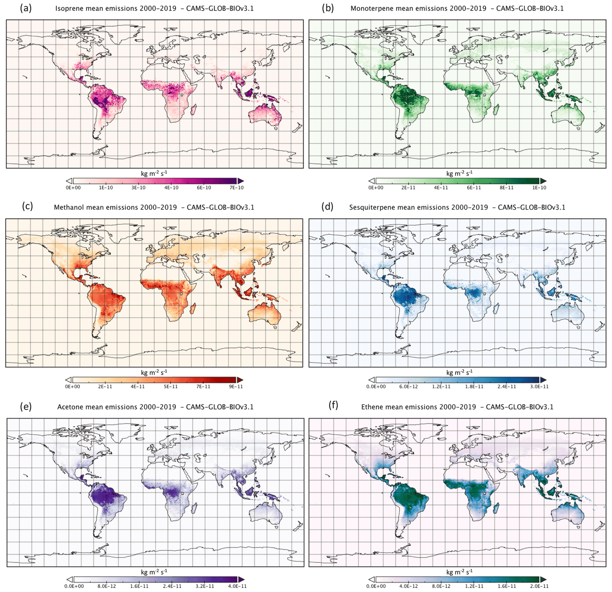
Figure 1 Spatial distribution of emissions averaged over the 2000–2019 period for (a) isoprene, (b) sum of monoterpenes, (c) methanol, (d) sum of sesquiterpenes, (e) acetone and (f) ethene in the CAMS-GLOB-BIOv3.1 dataset.

The global spatial distribution of CAMS-GLOB-BIOv3.1 emissions for selected species is presented in Fig. 1. Regions of highest emission are located in the tropical band and include Amazonia, Central Africa, Southeast Asia, Indonesia and northern Australia.

Additionally, significant BVOC emission sources are located in the south-eastern part of the US, especially during the summer months of the Northern Hemisphere. Substantial quantities of monoterpenes and methanol are further emitted from the northern temperate and boreal forests. BVOC emissions have strong seasonal variation following local meteorological conditions and a vegetation cycle with the highest emissions during daytime and in the summer season and the lowest emissions during nighttime and winter months.

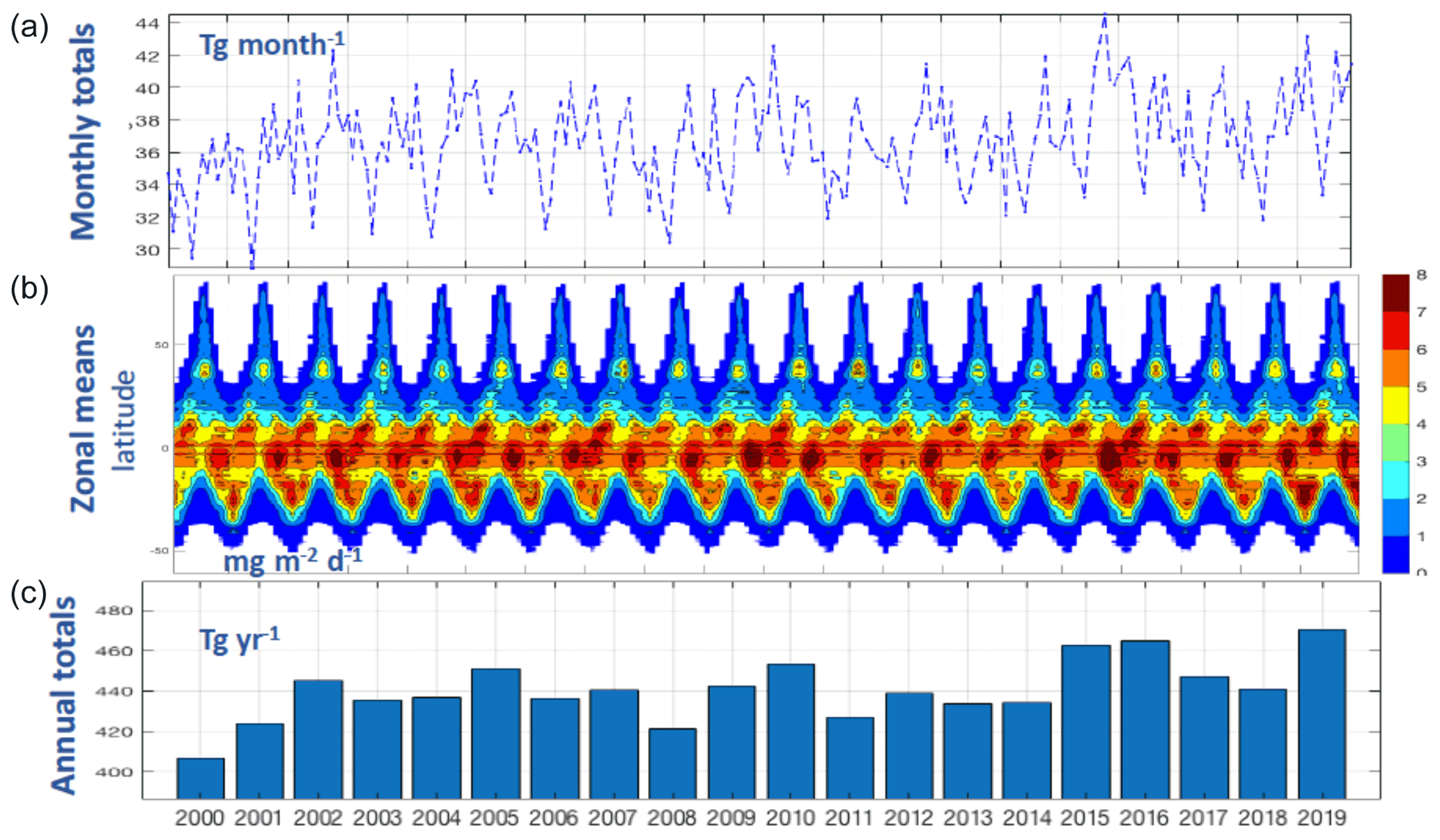
Figure 2 Global monthly totals (a), zonal means (b) and global annual totals (c) of the isoprene emissions for the period of 2000–2019 in the CAMS-GLOB-BIOv3.1 inventory.

Temporal variations in isoprene, the most abundant BVOC species, for the period of 2000–2019 from the CAMS-GLOB-BIOv3.1 dataset are presented in Fig. 2. The plot shows global monthly totals and interannual variation in emissions as well as isoprene zonal means. The zonal means stress again the tropical and southern subtropical band as the most important source of global isoprene, with additional sources in northern temperate latitudes.

The interannual changes in emissions are driven partially by interannual changes in vegetation through changes in leaf area index but to a greater extent by interannual changes in meteorology. There is a clear link between emissions and El Niño and La Niña phenomena. Annual global totals as well as zonal means in Fig. 2 show an isoprene decrease in 2008 and 2011, when strong La Niña was identified, and an increase in 2002, 2015 and 2019 during El Niño episodes. Such a connection between BVOC emissions and El Niño phenomena was already noted in previous studies (e.g. Naik et al., 2004; Müller et al., 2008; Wells et al., 2020).

Table 6 Regional annual emissions for CAMS-GLOB-BIOv3.1 isoprene, monoterpenes, methanol, acetone, sesquiterpenes and ethene expressed as Tg (species) yr⁻¹ and as a percentage of the global total.

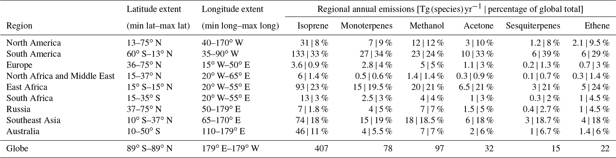
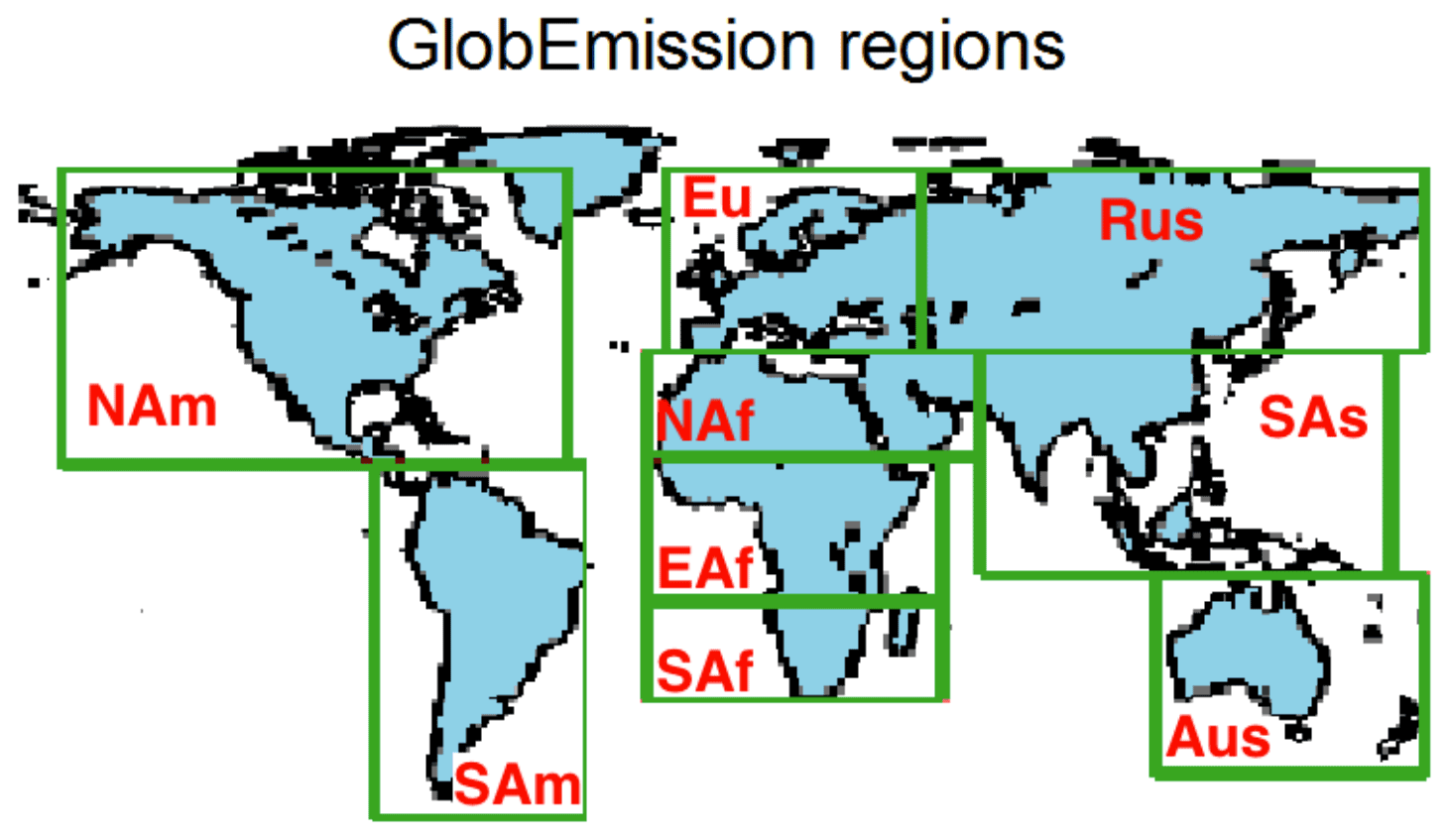
Figure 3 Geographical extent of the GlobEmission regions. Adapted from GlobEmission (https://www.globemission.eu/, last access: 18 January 2022).

3.2 Regional distribution of emissions

The CAMS-GLOB-BIOv3.1 emissions of the main BVOC species for the year 2000 were further analysed to show their regional contribution to global totals. We have used regions defined under the GlobEmission project (https://www.globemission.eu/, last access: 18 January 2022) which divide the globe to nine emitting areas. The spatial extent of the regions is given in Table 6 and shown in Fig. 3.

Table 6 presents the annual emission of isoprene, monoterpenes, methanol, acetone, sesquiterpenes and ethene from each of the regions together with their relative contribution to the global total. For all species (except for methanol), more than 70 % of emissions originate in tropical regions of South America, East Africa and Southeast Asia and 10 %–18 % of emissions have their source in the northern latitudes (North America, Europe and Russia). When compared to other species, a production of isoprene is especially low in Europe and Russia, with less than 1 % and 2 % of the global total, respectively. For methanol, the tropics contribute with only 63 %, and almost 25 % of methanol is produced in the northern latitudes, mainly in North America and Russia.

3.3 Impact of land cover change on isoprene emissions

The impact of changing land cover on emissions is captured in the CAMS-GLOB-BIOv3.0 dataset. To illustrate the effect of changing land cover on isoprene, the 20-year time series of isoprene annual totals was fitted with a linear regression trend and compared to data from v3.1, for which a static CLM4 land cover map was used. When calculated with the static vegetation map, isoprene emissions increase globally by 0.35 % yr⁻¹ due to temporal changes in meteorology. When annually changing ESA-CCI data are implemented, the trend decreases to 0.24 % yr⁻¹. A similar observation was made by Opacka et al. (2021), who used a modified MODIS land cover data in the MEGAN-MOHYCAN emission model to study the impact of land cover change on isoprene emissions. They found a 0.04 to 0.33 % yr⁻¹ mitigating effect of land cover change on general positive trends of isoprene induced mainly by temperature and solar radiation.

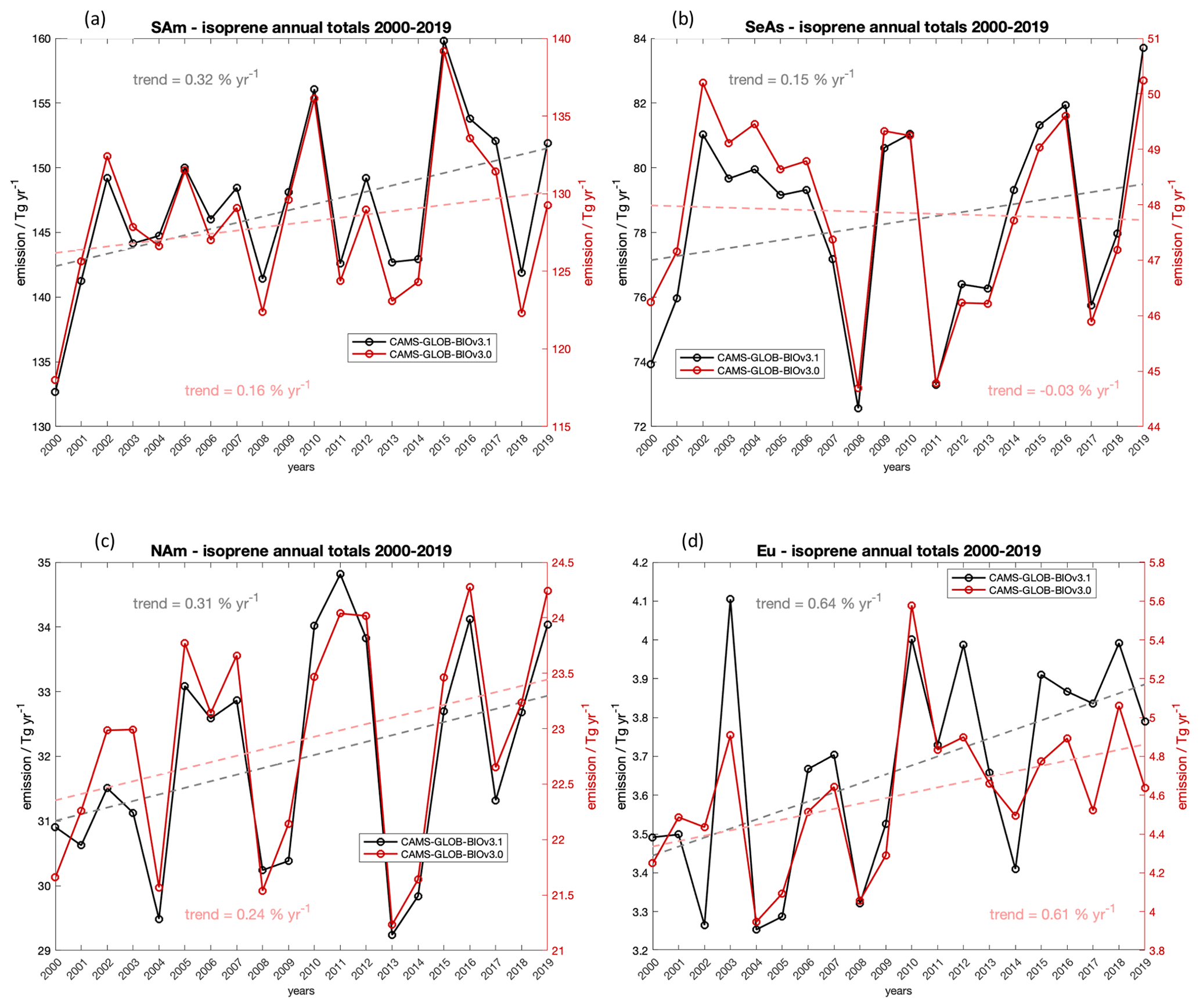
Figure 4 Comparison of isoprene annual totals from CAMS-GLOB-BIOv3.0 and v3.1 in (a) South America, (b) Southeast Asia and Indonesia, (c) North America, and (d) Europe with linear trend for each dataset (dashed line and trend value in % yr⁻¹).

Figure 4 presents a comparison of the v3.0 and v3.1 isoprene emission trends in selected regions. The regions' definition and spatial extent are given in Table 6. Inclusion of land cover change through ESA-CCI data (v3.0) reduces isoprene trends in South America (especially in the Amazon) or even causes a negative isoprene trend in Southeast Asia when compared to v3.1 based on static land cover. Such a trend decline is caused mainly by a retreat of tropical broadleaf forest (broadleaf evergreen and deciduous trees) in these locations. On the other hand, we observe an increase in the isoprene trend in East Africa, North Africa and the Middle East, and Russia, where the ESA-CCI data show an increase in the broadleaf deciduous tree category (tropical and boreal) in the course of the 20-year period. A moderate decrease in the isoprene trend (relative difference of −20 % to −30 %) can be observed in North America, South Africa and Australia, and the trend remains almost unchanged between the v3.0 and v3.1 data in Europe.

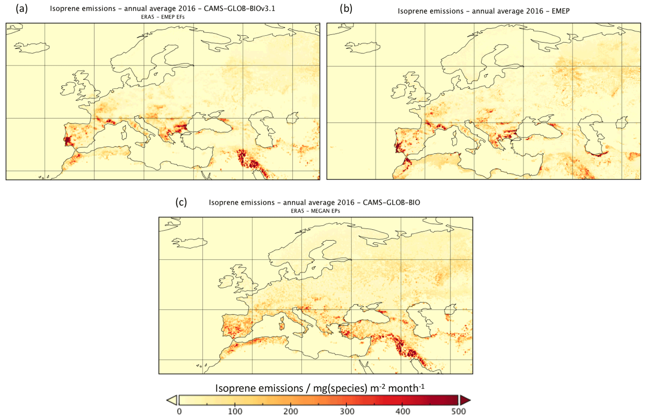
Figure 5 Comparison of European annual mean isoprene emissions in 2016 from (a) the EMEP model and (b) CAMS-GLOB-BIOv3.1. Panel (c) shows annual mean isoprene emissions calculated with default MEGAN EP maps.

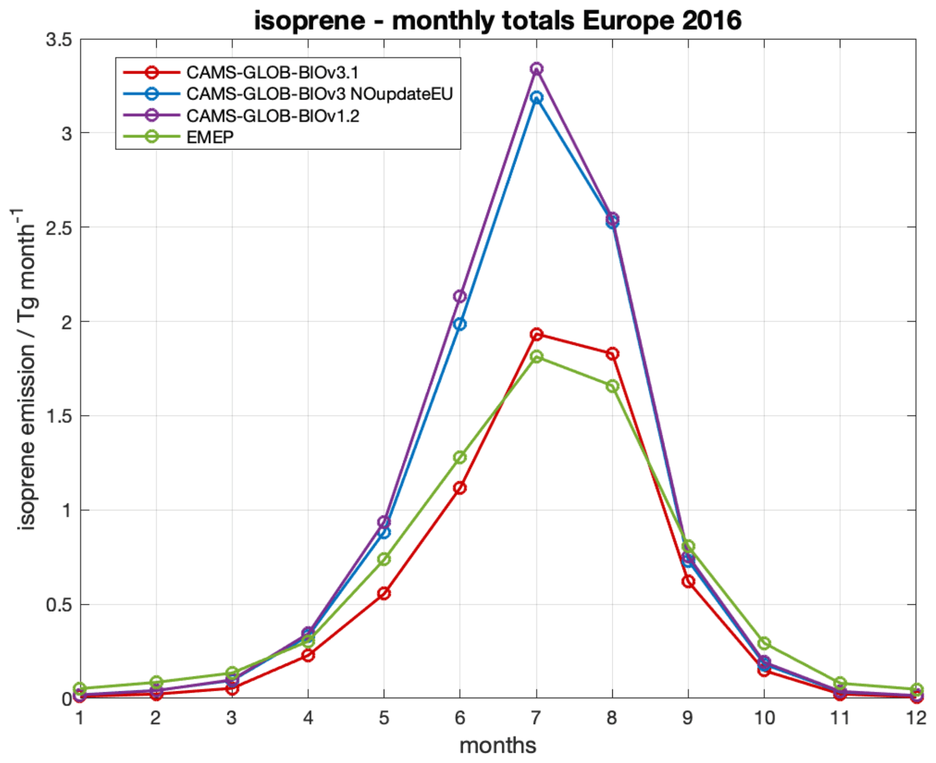
Figure 6 Isoprene monthly totals in Europe in the year 2016 from CAMS-GLOB-BIO datasets (v3.1, v3.1 without EP update and v1.2) and EMEP model.

3.4 Isoprene emission update in Europe

Updated isoprene emission potential values in Europe, described in more detail in Sect. 2.5, were used to calculate isoprene emissions in CAMS-GLOB-BIOv3.1. The spatial distribution of annual mean isoprene emissions in Europe is presented in Fig. 5, where CAMS-GLOB-BIOv3.1 emissions are compared with emissions obtained directly from the EMEP model (v4.33; Simpson et al., 2019) and with isoprene emissions calculated with similar settings in MEGAN as v3.1 (i.e. meteorology, PFT distribution, LAI) but using the MEGAN default emission potential maps instead of the updated EPs.

Figure 5 shows a good agreement in spatial distribution and quantity of calculated emissions between the EMEP and v3.1 emissions, which supports the approach of updated EP calculation and conversion from EMEP inputs to MEGAN format. It can also be seen that the spatial distribution of isoprene emissions changes when updated EPs are applied. Emissions calculated with MEGAN default EPs are more uniformly distributed over the European domain, while v3.1 emissions are more localized, with isoprene hotspots in areas covered by highly emitting tree species, e.g. in Portugal, Spain, southern France and the Balkan Peninsula.

Use of updated instead of MEGAN default EPs in Europe leads to a 35 % decrease in isoprene annual total from 10.03 Tg yr⁻¹ (v3.1 without EP update) to 6.55 Tg yr⁻¹ (v3.1). Isoprene monthly totals from these two datasets are compared to CAMS-GLOB-BIOv1.2 (annual total of 10.5 Tg yr⁻¹) and to isoprene estimated by EMEP (7.3 Tg yr⁻¹) in Fig. 6. The plot shows a clear decrease in emissions after use of the updated EPs and a good agreement between the CAMS-GLOB-BIOv3.1 and EMEP estimates. The results were extracted for the European domain with latitudes from 30.5–71.75^∘ N and longitudes from 29.75^∘ W to 65.75^∘ E.

3.5 Comparison of CAMS-GLOB-BIO emissions with other inventories

Time series of CAMS-GLOB-BIO emissions of isoprene and monoterpenes were compared to other available data. We focus on isoprene and monoterpenes as these are the two most abundant BVOC species and the two species for which time series from other sources are available. The rest of the species unfortunately suffer from lack of available and time-varying data.

Table 7 List of datasets used for comparison of emissions.

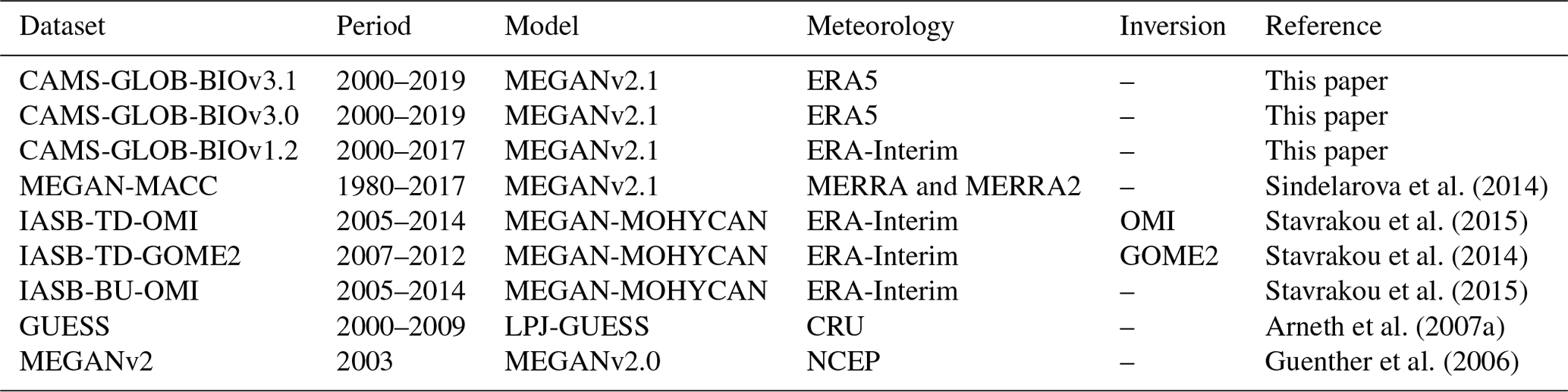
Datasets gathered for this comparison are listed in Table 7. Each dataset is assigned with basic information such as model used for emission estimation and driving meteorology. Most of the inventories are so-called “bottom-up” inventories, i.e. modelled by an emission model based on meteorology, emission factors and vegetation distribution. There are two “top-down” datasets, IASB-TD-OMI and IASB-TD-GOME2, which were calculated by an emission model and then constrained with satellite observations of formaldehyde (from OMI and GOME2) by applying an inversion technique in the chemical transport model (IMAGESv2) (Stavrakou et al., 2014, 2015). Most of the inventories were calculated with a “MEGAN-like” emission model algorithm except for the GUESS dataset, which was estimated by a process-based model LPJ-GUESS (Smith et al., 2001; Sitch et al., 2003). The IASB datasets were obtained from the website of the GlobEmission project (http://www.globemission.eu/, last access: 18 January 2022). The rest of the data were obtained from the ECCAD database (http://eccad.aeris-data.fr/, last access: 18 January 2022).

Figures 7 and 8 show a comparison of isoprene and monoterpene annual totals within the 2000–2019 period, respectively. In both cases, the CAMS-GLOB-BIO emissions fall well within the range of other estimates. Though both plots show there is quite a large spread between the datasets, with maximal differences up to a factor of 2 to 3 (difference of 320 Tg yr⁻¹ for isoprene and 61 Tg yr⁻¹ for monoterpenes). There are various reasons for these discrepancies, the most important being selection of the emission model, driving meteorology and input vegetation data (land cover description and emission factors).

In this data collection, the highest isoprene and monoterpene emissions are estimated by the MEGAN-MACC dataset. This dataset was calculated based on the MERRA and MERRA2 reanalyses (Rienecker et al., 2011) and therefore differs in the use of meteorological inputs from most of the remaining datasets which used ERA meteorological fields (ERA-Interim and ERA5). Comparison of 2 m temperature and PAR fields from the MERRA and ERA datasets showed higher values of both meteorological parameters in the MERRA dataset mainly in the tropical regions of South America, Central Africa and Australia, i.e. locations of high BVOC emission potential. Higher temperature and PAR values in MERRA data then result in higher MEGAN-MACC estimates.

The key role of meteorology in BVOC estimation is supported also by a relatively good agreement of CAMS-GLOB-BIOv1.2 isoprene emissions with IASB datasets, especially IASB-BU-OMI and IASB-TD-GOME2, which are both calculated based on ERA-Interim fields. Furthermore, the impact of meteorological inputs can also be observed in the difference between CAMS-GLOB-BIOv1.2 and v3.1 estimates based on ERA-Interim and ERA5, respectively, which is discussed in Sect. 3.1.

Interannual variability for most of the datasets is similar as they are mostly driven by the ERA meteorology, again except for MEGAN-MACC, based on MERRA reanalysis, for which the amplitude is higher. For all datasets there is a clear link between isoprene emissions and El Niño and La Niña phenomena. As also presented in Fig. 2, isoprene emissions decrease in 2008 and 2011 during strong La Niña and increase in 2002, 2015 and 2019 during El Niño episodes.

For monoterpenes the interannual variability is not as profound as for isoprene. Similar to isoprene, monoterpenes are strongly emitted in the tropical region but also have significant sources in the temperate and boreal forests in the Northern Hemisphere. As a result, they are not as susceptible to atmospheric changes in the tropical band as isoprene and keep a rather stable interannual profile.

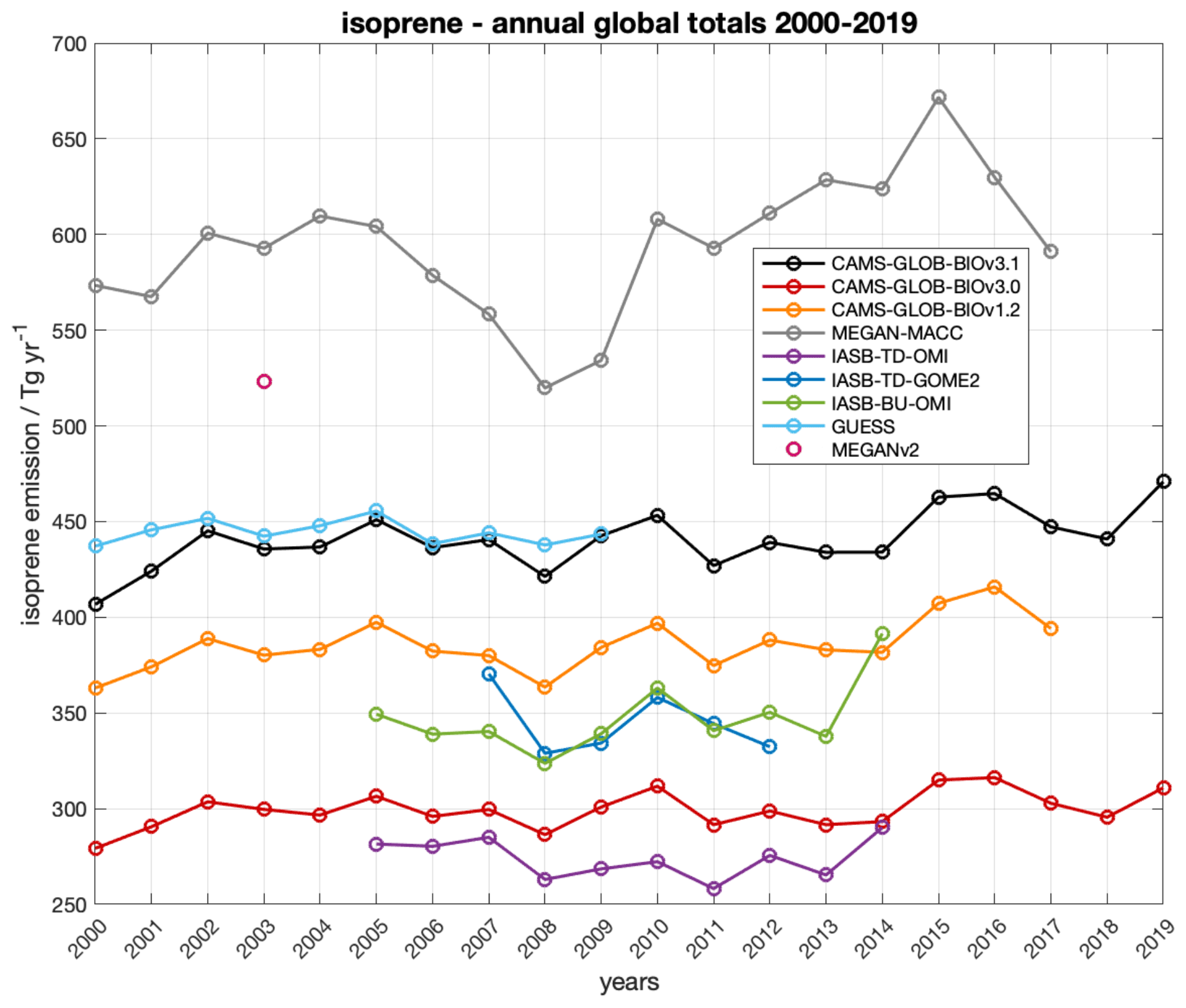
Figure 7 Comparison of isoprene global annual totals from CAMS-GLOB-BIOv3.1 (black), CAMS-GLOB-BIOv3.0 (red), CAMS-GLOB-BIOv1.2 (orange) and other available inventories within the 2000–2019 period.

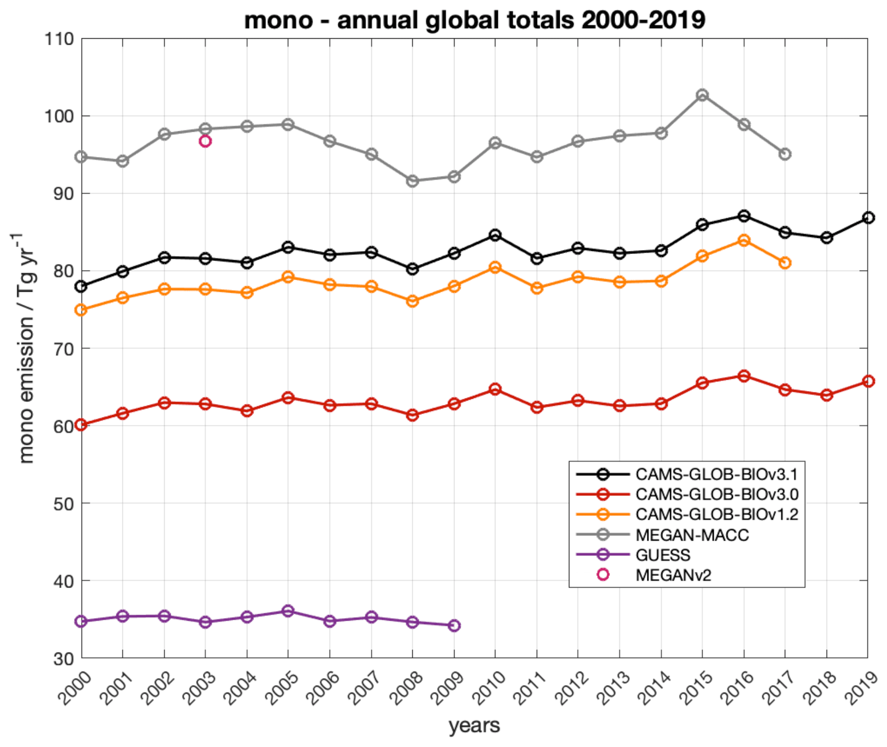
Figure 8 Comparison of monoterpene global annual totals from CAMS-GLOB-BIOv3.1 (black), CAMS-GLOB-BIOv3.0 (red), CAMS-GLOB-BIOv1.2 (orange) and other available inventories within the 2000–2019 period.

4 Data availability

Gridded maps with global emissions per species available as monthly means or monthly averaged daily profiles are provided as NetCDF (Network Common Data Format) files for the global domain at a resolution of 0.5^∘ × 0.5^∘ (CAMS-GLOB-BIOv1.2, https://doi.org/10.24380/t53a-qw03, Sindelarova et al., 2021a) and at a resolution of 0.25^∘ × 0.25^∘ (CAMS-GLOB-BIOv3.0, https://doi.org/10.24380/xs64-gj42, Sindelarova et al., 2021b; CAMS-GLOB-BIOv3.1, https://doi.org/10.24380/cv4p-5f79, Sindelarova et al., 2021c) and can be accessed through the Emissions of atmospheric Compounds and Compilation of Ancillary Data (ECCAD) system with a login account (https://eccad.aeris-data.fr/, last access: June 2021). For review purposes, ECCAD has set up an anonymous repository where subsets of the CAMS-GLOB-BIOv1.2, CAMS-GLOB-BIOv3.0 and CAMS-GLOB-BIOv3.1 data can be accessed directly (https://eccad.aeris-data.fr/essd-surf-emis-cams-bio/, last access: June 2021).

5 Conclusions

The presented paper describes three new global inventories of biogenic volatile organic compounds emitted from vegetation which are publicly available for use by the air quality and climate models. The datasets are called CAMS-GLOB-BIO v1.2, v3.0 and v3.1 and were calculated with the Model of Emissions of Gases and Aerosols from Nature (MEGANv2.1) driven by meteorological reanalyses of the European Centre for Medium-Range Weather Forecasts (ECMWF). Inventories include emissions of 25 BVOC species or chemical groups provided as monthly means and monthly averaged daily profiles spanning the period of 2000–2019. The CAMS-GLOB-BIO datasets were developed under the Copernicus Atmosphere Monitoring Service project (CAMS; global and regional emissions) as part of the European Union's Copernicus Earth Observation Programme.

The dataset CAMS-GLOB-BIOv1.2 is based on ERA-Interim meteorological fields and is available with a horizontal spatial resolution of 0.5^∘ × 0.5^∘. The datasets CAMS-GLOB-BIOv3.1 and v3.0 were calculated with ERA5 meteorology and are provided with a horizontal spatial resolution of 0.25^∘ × 0.25^∘.

CAMS-GLOB-BIOv3.1 estimates global annual total BVOC emission of 591 Tg (C) yr⁻¹, with isoprene as the main contributing species (440.5 Tg (isoprene) yr⁻¹). Use of ERA5 meteorology in v3.1 leads to a slight increase in BVOC emissions compared to v1.2, with a global BVOC total of 532 Tg (C) yr⁻¹ (including 385.2 Tg (isoprene) yr⁻¹). The total emission in the CAMS-GLOB-BIOv3.0 dataset is 424 Tg (C) yr⁻¹, with isoprene emissions of 299.1 Tg (isoprene) yr⁻¹. The difference between v3.1 and v3.0 estimates can mostly be attributed to use of an alternative land cover map for the vegetation description.

CAMS-GLOB-BIOv3.1 includes isoprene estimates in Europe calculated with an updated map of emission potential values which are based on fine-scale land cover with detailed maps of tree species and should therefore better represent the composition of European forests than the global EP maps of the MEGAN model. Use of updated isoprene EP maps led to a substantial decrease in the European isoprene emission total by 35 % and caused a change in spatial distribution of emissions. Isoprene emissions are concentrated in several emission hotspots in locations covered by highly emitting tree species.

Both v3.1 and v1.2 estimates are based on a static land cover description obtained from the Community Land Model (CLM4). Since the world's vegetation is experiencing significant changes, such as deforestation in the tropical region, replacement of forests by agricultural land and afforestation efforts with fast-growing trees, we aimed to take this effect into account. The CAMS-GLOB-BIOv3.0 dataset considers changes in global land cover by using the ESA-CCI annual land cover maps for the vegetation description in the MEGAN model. In order to use a new land cover input in the model, the emission potentials had to be calculated from the PFT distribution instead of using the high-resolution emission potential maps. Such a difference in input EP data and a different input land cover map (ESA-CCI instead of CLM4) caused a decrease of ∼ 30 % for annual total isoprene and ∼ 20 % for monoterpenes when compared to CAMS-GLOB-BIOv3.1. The linear trend analysis of the 20-year time series of global isoprene emissions showed that inclusion of time-varying land cover data causes a decrease in the general isoprene growing trend from 0.35 to 0.24 % yr⁻¹. The trend slowdown is even more profound in the tropical regions of South America and Southeast Asia, where according to ESA-CCI data the retreat of tropical broadleaf forest can be observed. On the other hand, due to expansion of broadleaf deciduous trees the increasing isoprene trend is intensified in regions such as East and Central Africa or Russia.

Time series of CAMS-GLOB-BIO isoprene and monoterpene emissions were compared to other available data. The estimates fall well within the range of values from other studies. However, the comparison shows there is quite large uncertainty in emission estimates, which on a global scale can reach up to a factor of 2 to 3, with even higher values on a regional level. The different emission estimates in different versions of the CAMS-GLOB-BIO datasets provide the uncertainty's main driving factors, i.e. meteorological inputs, definition of input emission potentials and land cover distribution.

The presented CAMS-GLOB-BIO datasets provide high-resolution data of global BVOC emissions for the period of 20 recent years based on up-to-date input data. The datasets are suitable for the purposes of air quality modelling, especially for models that do not include their own module for online BVOC emission estimation. Our general recommendation is to use a CAMS-GLOB-BIO dataset which is calculated with the same meteorology as the one that drives the air quality model. If this does not apply, we recommend using the latest CAMS-GLOB-BIOv3.1 dataset. CAMS-GLOB-BIOv3.0 should be used for studies focusing on land cover change.