the Creative Commons Attribution 4.0 License.
the Creative Commons Attribution 4.0 License.
 | 12 May 2022
Greenland Geothermal Heat Flow Database and Map (Version 1)
Agnes Wansing
Kenneth Mankoff
Mareen Lösing
John Hopper
Keith Louden
Jörg Ebbing
Flemming G. Christiansen
Thomas Ingeman-Nielsen
Lillemor Claesson Liljedahl
Joseph A. MacGregor
Árni Hjartarson
Stefan Bernstein
Nanna B. Karlsson
Sven Fuchs
Juha Hartikainen
Johan Liakka
Robert S. Fausto
Dorthe Dahl-Jensen
Anders Bjørk
Jens-Ove Naslund
Finn Mørk
Yasmina Martos
Niels Balling
Thomas Funck
Kristian K. Kjeldsen
Dorthe Petersen
Ulrik Gregersen
Gregers Dam
Tove Nielsen
Shfaqat A. Khan
Anja Løkkegaard
We compile and analyze all available geothermal heat flow measurements collected in and around Greenland into a new database of 419 sites and generate an accompanying spatial map. This database includes 290 sites previously reported by the International Heat Flow Commission (IHFC), for which we now standardize measurement and metadata quality. This database also includes 129 new sites, which have not been previously reported by the IHFC. These new sites consist of 88 offshore measurements and 41 onshore measurements, of which 24 are subglacial. We employ machine learning to synthesize these in situ measurements into a gridded geothermal heat flow model that is consistent across both continental and marine areas in and around Greenland. This model has a native horizontal resolution of 55 km. In comparison to five existing Greenland geothermal heat flow models, our model has the lowest mean geothermal heat flow for Greenland onshore areas. Our modeled heat flow in central North Greenland is highly sensitive to whether the NGRIP (North GReenland Ice core Project) elevated heat flow anomaly is included in the training dataset. Our model's most distinctive spatial feature is pronounced low geothermal heat flow (< 40 mW m−2) across the North Atlantic Craton of southern Greenland. Crucially, our model does not show an area of elevated heat flow that might be interpreted as remnant from the Icelandic plume track. Finally, we discuss the substantial influence of paleoclimatic and other corrections on geothermal heat flow measurements in Greenland. The in situ measurement database and gridded heat flow model, as well as other supporting materials, are freely available from the GEUS Dataverse (https://doi.org/10.22008/FK2/F9P03L; Colgan and Wansing, 2021).
- Article
(17883 KB) - Full-text XML
- BibTeX
- EndNote


Assessing the magnitude and spatial distribution of geothermal heat flow across Greenland is important for many reasons, such as mapping geothermal springs and energy resources; constraining a key basal boundary condition for the permafrost, glaciers, and the ice sheet; constraining the thermal structure and material properties of the lithosphere; and understanding the generation and preservation of hydrocarbon accumulations. However, the current generation of Greenland regional heat flow models still shows substantial disagreement (Rezvanbehbahani et al., 2017; Martos et al., 2018; Greve, 2019). A fundamental challenge in reliably interpolating the magnitude and spatial distribution of geothermal heat flow across Greenland is the paucity of local heat flow measurements with which to constrain regional heat flow models.
Of the 40 870 onshore heat flow measurements presently catalogued in the International Heat Flow Commission (IHFC) database, just 10 (∼ 0.02 %) are onshore in Greenland (Fuchs et al., 2021a). As Greenland represents ∼ 1.5 % of global land area, this makes the country disproportionately underrepresented in the IHFC database. While several studies have assembled additional non-IHFC heat flow measurements from published sources (Martos et al., 2018; Rysgaard et al., 2018), it is highly desirable to have a comprehensive and continuously updated open-access repository of all Greenland heat flow measurements. It is similarly desirable to have an open-access Greenland heat flow map that is self-consistent with that updating repository.
The goal of this study is to develop and describe this first version of the Greenland Geothermal Heat Flow Database and Map. First, we collect existing and new heat flow measurements in and around Greenland into a database with uniform metadata. Second, we apply machine learning to this database, along with other geophysical datasets, to produce a regional model of the magnitude and spatial distribution of Greenland heat flow that is consistent with these measurements. These data products and their supporting information are publicly available. We anticipate updating the heat flow database and map as new measurements become available. Here, we describe the development of these data products and discuss their implications for advancing our understanding of Greenland's geothermal heat flow.
2.1 Heat flow measurement database
We use the 2018 IHFC database as the foundation upon which to build a region-specific update of Greenland heat flow measurements. This 2018 version of the IHFC database, which contains 58 536 measurements (both onshore and offshore) with no quality documentation, is an updated version of the 2013 IHFC database (Global Heat Flow Compilation Group, 2013; https://doi.org/10.1594/PANGAEA.810104). Within our Greenland domain, the IHFC 2018 database contains 290 heat flow measurements, the majority of which are offshore (Fig. 1). In 2021, the fundamental structure of the IHFC database was revised for the first time since 1976 (Jessop et al., 1976; Fuchs et al., 2021b). While the previous 1976 IHFC database structure contained 17 data fields for each heat flow measurement, the new 2021 IHFC database structure now contains 59 data fields for each heat flow measurement, 18 of which are “mandatory”, 32 of which are “recommended”, and 9 of which are “optional”. The novel heat flow database we present here has 26 data fields for each heat flow measurement. Eighteen of these fields have 100 % data coverage, but these do not align with all 18 “mandatory” IHFC 2018 fields (Table A1). Four fields, associated with the temperature gradient, depth range, and thermal conductivity, have better than 81 % data coverage. The last four fields, associated with topographic correction of heat flow, have 34 % data coverage.
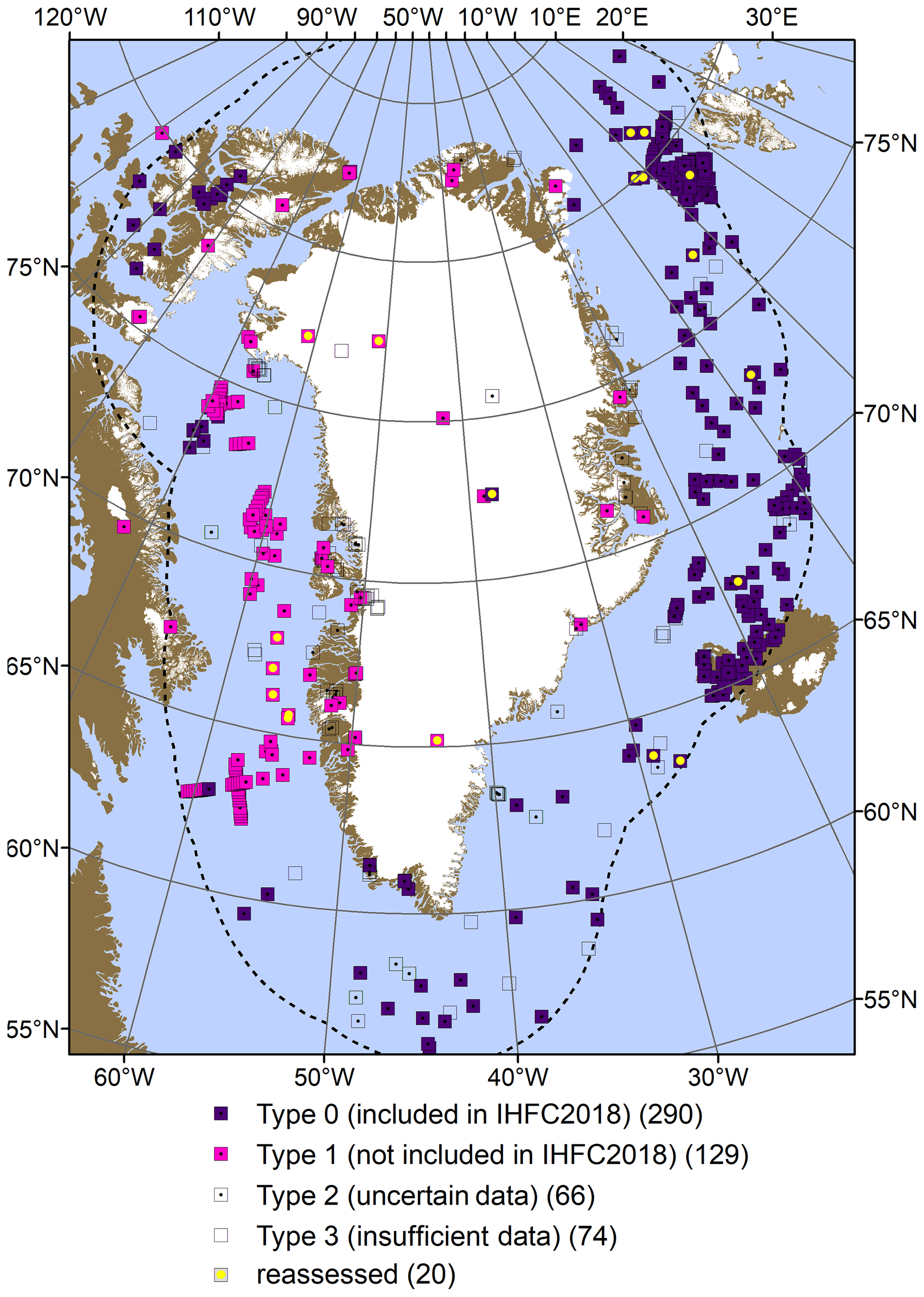
Figure 1Overview of site locations and types in the heat flow measurement database. Reassessed heat flow values described in Tables 3 and 4. Dashed line denotes our study boundary, 500 km from Greenland's coasts. The Meighen and Barnes ice caps lie outside this boundary, but we still report these subglacial measurements here. Projection is EPSG:3413. See Fig. 6 for the sites overlaid on a bathymetric map.
We briefly introduce and describe the fields of our database in Table 1. While our database generally exceeds the information required by the IHFC 1976 database structure, it does not contain 8 of the 18 mandatory fields of information required by the IHFC 2021 database structure (Table A1). Conforming and assimilating our database into the IHFC 2021 database and structure remains a near-term but non-trivial goal. While translating the “measurement type” of this study into “geographical environment” of IHFC 2021 is relatively straightforward, assessing IHFC 2021 fields like “TC saturation” or “TC pT conditions” (where TC refers to thermal conductivity, and pT refers to pressure and temperature) requires reviewing historical measurements on a site-by-site basis. Similar to the IHFC databases, however, our present database has a “one borehole, one estimate” philosophy. This merges multiple estimates for a single borehole into a single best or consensus estimate for that borehole. Generally, for the predominantly subglacial sites where multiple estimates have been published, the consensus estimate is reached by expert elicitation within our author team. Further, our database only includes direct heat flow estimates: those derived from temperature gradient measurements. Following the IHFC, we exclude heat flow estimates derived from remotely sensed approaches (i.e., Cox et al., 2021).
Generally, our present database has a greater focus on three-dimensional positional accuracy than the IHFC databases. We report positions, elevations, and uncertainties in both latitude–longitude and the popular EPSG:3413 coordinate system adopted by many Greenland-focused and Arctic-wide data products. The EPSG:3413 system, also known as the NSIDC Sea Ice Polar Stereographic North projection, has its latitude of origin at 70∘ N and its central meridian at 45∘ W and provides a polar projection for data products (see: http://epsg.io/3413; last access: 8 February 2022). This focus on three-dimensional positional uncertainty is intended to facilitate future investigations of local heat flow corrections, such as those associated with paleoclimate or topography. As Greenland is a high-relief land mass with a complex climate history, these corrections are likely more important in modifying contemporary heat flow measurements in Greenland than lower-relief and more temperate regions of Earth.

2.2 Heat flow measurements
Heat flow measurements typically rely on knowledge of local temperature gradient and local thermal conductivity, with the product of these two terms yielding heat flow. There can be substantial diversity in the depth interval over which temperature gradient is measured, from kilometer-scale deep boreholes to meter-scale heat probes. Similarly, there can be substantial diversity in how thermal conductivity is estimated, ranging from relatively precise continuous-core laboratory analysis to less precise estimations based on tabulated data from analogous rock types. For this reason, it is desirable to present a heat flow measurement with sufficient metadata for users to assess the relative differences in data quality between sites (Table 1). In this database, we assess uncertainty in heat flow based on the quality of the local temperature gradient and thermal conductivity data comprising the heat flow. In the following, all mentions of “conductivity” relate to “thermal conductivity”. We divide the heat flow measurements into four types: Type 0 contains measurements already included in IHFC 2018, Type 1 contains “new” measurements that are not included in IHFC 2018, Type 2 contains sites for which we are uncertain if sufficient data exist to estimate heat flow, and finally Type 3 contains sites where we feel there are insufficient data to estimate heat flow with available methods.
2.2.1 Type 0 – included in IHFC 2018
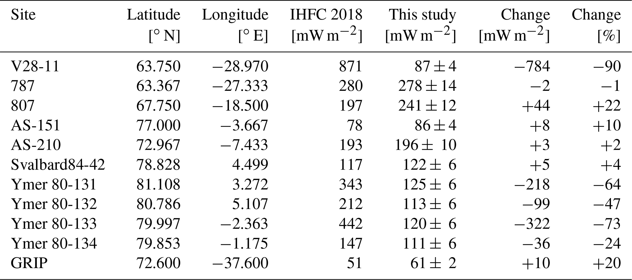
The IHFC 2018 database contains 290 heat flow measurements within our Greenland domain (Fig. 1). Here, we provide the first systematic quality control of these existing IHFC data, as part of a broader community effort to bring all historical IHFC into compliance with the most recent IHFC data standards (Fuchs et al., 2021a). During this quality control, we reassess 10 of these historical IHFC heat flow values in our present database (Table 2). The remaining 280 historical IHFC heat flow measurements are unchanged.
The largest reassessment is site V28-11. The heat flow at this site – 871 mW m−2 – is a clear outlier within the IHFC 2018 database, exceeding the next highest value within the Greenland region by a factor of 2. It is also more than an order of magnitude greater than the contemporaneous measurement at V30-96, located 72 km away. While all temperature gradients measured during the V28 and V30 cruises range between 35 and 181 K km−1, the V28-11 temperature gradient is listed as 1000 K km−1 in IHFC 2018. Such an extreme heat gradient seems implausible (Bons et al., 2021). We attribute this to a transposed decimal place and revise the gradient to a more reasonable 100 K km−1. This accordingly reassesses the V28-11 heat flow to 87 mW m−2. In comparison, the nearby V30-96 heat flow measurement is 52 mW m−2.
There are nine other heat flow measurements where the product of reported gradient and conductivity is more than ±2 mW m−2 different from the reported heat flow. In these instances, heat flow has been revised to reflect the product of reported gradient and conductivity. This approach assumes that gradient and conductivity are the primary measurements from which heat flow is a secondarily derived product. The discrepancy of this reassessment of reported gradient and conductivity product is greatest at Ymer 80-133, where heat flow is reassessed from 442 to 120 mW m−2. Table 2 summarizes all instances of reassessed IHFC 2018 heat flows. Generally, these reassessments can be described as down-revising extreme heat flow values from oceanographic surveys conducted in the vicinity of the Mid-Atlantic Ridge in the late 1970s and early 1990s. These reassessments are also noted in the comments section of each entry in the database.
This study adds significant metadata to many of the existing IHFC 2018 entries. First, all 290 existing IHFC 2018 entries are coded as either “subaerial”, “submarine”, or “subglacial”. Heat flow uncertainties are also estimated for all 290 sites. Where site-specific measurements of both temperature gradient and thermal conductivity are available, an uncertainty of ±5 % is assumed. Where only site-specific temperature gradient is measured, and thermal conductivity is assumed, an uncertainty of ±10 % is assumed. Where only heat flow is reported, without a specific temperature gradient or thermal conductivity, an uncertainty of ±15 % is assumed. This approach is applied to all Type 0 (and Type 1) sites for which formal uncertainties are not previously reported. For 50 of the existing Type 0 IHFC 2018 sites, a previously unavailable elevation of measurement is interpolated from a digital elevation model. Within the immediate proximity of Greenland, the higher-resolution BedMachine v3 elevation model is used (150 m horizontal resolution), while for areas more distal to Greenland, the lower-resolution ETOPO1 elevation model is used (1 arcmin or ∼ 1.8 km horizontal resolution; Amante, and Eakins, 2009; Howat et al., 2014; Morlighem et al., 2017). For a further 10 sites, corresponding to the “OU” cruise, measurement elevations were revised from a positive water depth to a negative ocean bottom elevation. Finally, for 51 of these existing sites, a previously unavailable measurement year is now estimated from the IHFC 2018 “year of publication” field.
In addition to these batch additions of metadata, we also revised existing site-specific metadata in several instances. This includes renaming two non-unique “Akureyri” sites as “Akureyri73” and “Akureyri91”, non-unique “Grundarfjordur” sites as “Grundarfjordur91A” and “Grundarfjordur91B”, and finally two non-unique “Hvammstangi” sites as “Hvammstangi73” and “Hvammstangi91”. The numeric suffixes are based on measurement year. We remove an apparent IHFC 2018 double entry of “V29-155”. For the GRIP (GReenland Ice core Project) ice core site, the measured elevation is revised from sea level (0 m elevation) to the observed ice–bed interface at 203 m elevation. For GRIP, the heat flow was also reassessed with the approach described in Sect. 2.2.2 to be consistent with the heat flow assessed for other subglacial sites.
Table 2Reassessed heat flows between IHFC 2018 and this study.
2.2.2 Type 1 – not included in IHFC 2018
Our database includes 129 heat flow values that were not included in IHFC 2018 (Fig. 1). Of these, 54 heat flow values are collected from previously published gray-literature reports or peer-reviewed articles (Classen, 1977; Colebeck and Gow, 1979; Van Tatenhove and Olesen, 1994; Müller et al., 2006; Taylor et al., 2006; Damm, 2010; Harper et al., 2011; Rysgaard et al., 2018; Hartikainen et al., 2021). In the database, the “source” field of these heat flow values is listed as “as published.” The remaining 75 heat flow values are previously unreported. While heat flow values have been previously published at a handful of these sites, we reassess these heat flows using a consistent methodology. In the database, the “source” field of these heat flow values is listed as the author of this study who is most familiar with this calculation. Below, we provide a brief overview of these 75 heat flow values.
The first type of new heat flow measurements in the database is submarine measurements (44 of 75 new values). Of these, 30 measurements were collected during cruise 2005-040 of the Canadian Coast Guard Ship Hudson. These measurements comprise east–west and north–south transects in water depths of between 1015 and 2550 m within the Davis Strait. These heat flow values were calculated from site-specific measurements of temperature gradient and thermal conductivity measured by a 4 m heat probe deployed in the uppermost layers of submarine sediments. For these heat-probe measurements, site-specific heat flow uncertainty is propagated from gradient and conductivity uncertainties.
The remaining 14 new submarine measurements are derived from deep marine exploration wells and cored boreholes drilled offshore West Greenland between 1976 and 2011. These wells are between 1148 and 4385 m deep and at water depths between 104 and 1508 m. For these sites, the temperature gradient is calculated from Horning-corrected bottom-hole temperature and an assumed top-hole temperature of 4 ∘C, reflecting assumed bottom water temperature. We assume that any seasonal cycle in bottom water temperatures at these sites is small in comparison to the temperature difference between the top- and bottom-hole temperatures. For the 14 deep exploration wells presented here, the average top-to-bottom temperature difference is 86 ∘C. In the absence of a method to systematically convert borehole stratigraphy into depth-integrated conductivity, we assume a bulk thermal conductivity of 2.00 W m−1 K−1 for all these deep boreholes. This approximates the back-calculated bulk thermal conductivity inferred by Rolle (1985) at five of these wells. We accordingly assume a 10 % uncertainty in heat flow at these sites.
Table 3Reassessed heat flows between previous studies and this study.
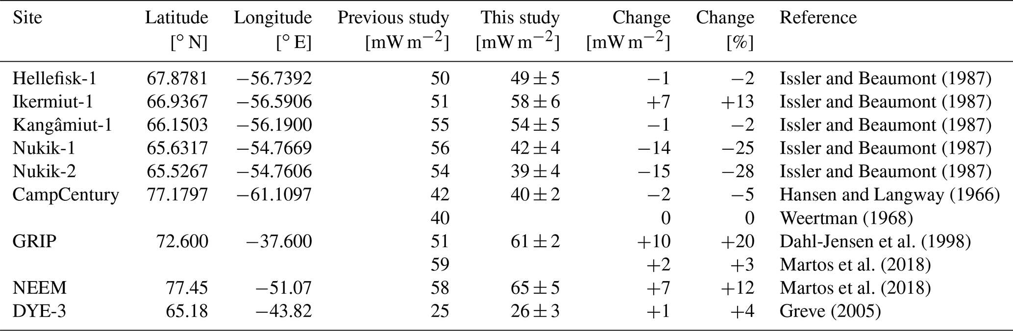
Issler and Beaumont (1987) previously estimated heat flows at five of these deep wells (Hellefisk-1, Ikermiut-1, Kangâmiut-1, and Nukik-1/2) that are generally higher than our heat flows (Table 3). While Issler and Beaumont (1987) do not provide the gradients or conductivities used in their calculations, the gradients we calculate are nearly identical to those published contemporaneously by Rolle (1985). We therefore speculate that the disparity between our heat flows and those of Issler and Beaumont (1987) results from differences in assumed conductivity.
The second type of new measurements in the database is subaerial measurements. This category specifically denotes ice-free onshore sites (11 of 75 new values). They are generally derived by applying an assumed thermal conductivity to a measured borehole temperature gradient. At three sites (DH-GAP01, Skaergaard_89-09B, and Skaergaard_90-11), thermal conductivity has also been measured (Balling and Brooks, 1991; Harper et al., 2011). At these sites, we estimate the uncertainty in heat flow from site-specific uncertainties in gradient and conductivity.
At the remaining eight sites, thermal conductivity has not been measured, so we must therefore assume a value (Roethlisberger, 1961; Dam and Christiansen, 1994; Van Tatenhove and Olesen, 1994; Bjerager et al., 2018). At sites located within the Precambrian Shield of southern Greenland (Alcoa_Site7e-I, Alcoa_Site7e-P, Alcoa_Site6g-P, SIS2019-02) we assume a thermal conductivity of 2.50 W m−1 K−1, based on the thermal conductivity measured near Kangerlussuaq (Harper et al., 2011). At sites located within the basaltic intrusions stretching across central Greenland from Disko Island to Geikie Plateau (G02_Paakitsoq, Marraat-1, Blokelv-1), we assume a thermal conductivity of 2.25 W m−1 K−1, based on thermal conductivity measured in the Skaergaard Formation (Balling and Brooks, 1991). At Thule (Thule_1002feet) we similarly assume a thermal conductivity of 2.25 W m−1 K−1, although with no guidance from measurements in analogous geological formations (Roethlisberger, 1961; Davies et al., 1963; Dawes, 2009). At all eight sites, we assume an uncertainty in heat flow of 10 %.
For all subaerial sites, where possible, we calculate temperature gradients below 75 m depth. As recent near-surface warming can decrease the near-surface temperature gradient and thus decrease near-surface heat flow in comparison to deeper values, we prefer not to use ground temperature data from depths shallower than 75 m. This approach minimizes the influence of recent, meaning post-1990, pronounced atmospheric warming on the near-surface temperature gradient (Balling and Brooks, 1991). This can be considered a basic paleoclimatic correction to remove the influence of recent climate change over the past century (Beltrami and Mareschal, 1991; Mareschal and Beltrami, 1992).
The third type of new measurements in the database is subglacial measurements (20 of 75 new heat flow values). This category specifically denotes onshore sites located beneath glaciers. Heat flow has been previously assessed at four of these sites (Table 3). For all subglacial sites, heat flow is calculated using a slightly modified version of the temperature gradient approach. We use ice temperature profiles from the Greenland Ice Borehole Temperature Profiles database (Mankoff, 2021; https://github.com/GEUS-PROMICE/greenland_ice_borehole_temperature_profiles, last access: 8 February 2022). At sites where the ice temperature profile is complete, meaning it spans the full ice thickness from surface to bed (Devon73, PrinceWales05, Meighen67, Agassiz77/79A/79B/84, Penny96, CampCentury, DYE-3, GISP2, NEEM, HansTausen_Dome, HansTausen_Hare), we fit a second-order temperature–depth function in the bottom 10 % of the borehole (Paterson, 1968; Weertman, 1968; Paterson et al., 1977; Fisher and Koerner, 1984; Gundestrup and Hansen, 1984; Clarke et al., 1987; Fisher et al., 1988; Clausen et al., 2001; Kinnard et al., 2008; Rasmussen et al., 2013; MacGregor et al., 2015). We then adopt the temperature gradient at the deepest 1 % of this second-order polynomial fit. This approach standardizes the approximation of temperature gradient across sites by accounting for differences in the depth interval of temperature measurements. It also acknowledges the characteristic non-linearity of basal ice temperature profiles (Hooke, 2019).
At some subglacial sites, however, the ice temperature profile is incomplete, meaning it does not reach the ice–bed interface (Devon72/98, Renland88, FladeIsblink06) (Paterson et al., 1977; Hansson, 1994; Kinnard et al., 2006; Lemark and Dahl-Jensen, 2010). At these sites, we must extrapolate the temperature profile to the ice–bed interface to approximate the temperature gradient in the deepest 1 % of the borehole. For this extrapolation, we generate a second-order polynomial fit to the deepest portion of the measured temperature–depth profile that is the same thickness as the depth range that is missing measurements, i.e., the depth range that must be extrapolated. For example, if ice temperatures are not available in the bottom 10 % of the borehole, then we fit the temperature–depth profile to the deepest available 10 % of the borehole where ice temperatures are available: the bottom 20 % down to the bottom 10 % of the borehole. This ensures a 1:1 ratio between the observation and extrapolation depth increments. To quantify the uncertainty associated with this extrapolation, we then repeat the extrapolation of the deepest 1 % gradient 10 times but adjust the shallowest depth of the data range up the ice column 1 % each time. We make available a sample of this code for the Devon72 extrapolation (Fig. 2) in the provided database associated with this article.
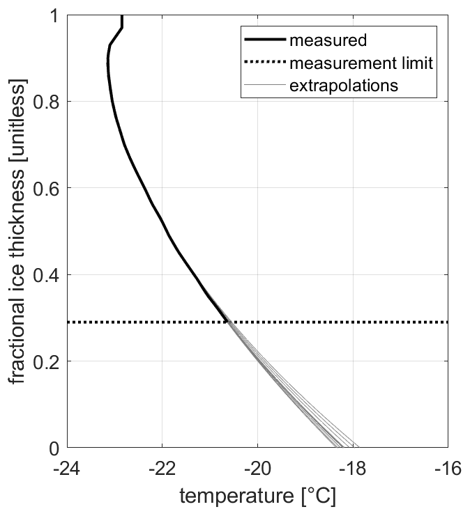
Figure 2Extrapolating temperature gradient at the ice–bed interface in the Devon72 borehole, where ice temperature measurements are not available in the deepest 29 % of the ice column.
For all subglacial boreholes, thermal conductivity (κ; in W m−1 K−1) is estimated as a function of ice temperature (Ti; in K) based on the following relation (Yen, 1981):
We prescribe the thermal conductivity of ice based on the ice temperature in the bottom 1 % of the borehole.
Four subglacial sites have unique glaciological settings requiring further explanation. Basal melting presently occurs at both NGRIP (North GReenland Ice core Project) and NEEM. This loss of basal ice is evident in local radiostratigraphy and depth–age relations at both sites. NGRIP has substantial basal melting, which prevents application of the basal-temperature-gradient approach described above. For this site, we estimate basal heat flow as 129 ± 30 mW m−2, based on the published range of values based on thermomechanical ice modeling (Dahl-Jensen et al., 2003; Greve, 2005; Buchardt and Dahl-Jensen, 2007). At NEEM, where there is evidence of trace basal melting, the basal-temperature-gradient approach is still valid, but we add a +5 ± 5 mW m−2 correction to account for an estimated 0.5 mm yr−1 of basal melt there (Rasmussen et al., 2013). At Tuto_D-11, the ice thickness is only 48 m. We therefore use a simple linear relation to constrain the temperature gradient in the lowermost 33 m of the ice, within a generous uncertainty from a digitized version of the published temperature profile (Davis, 1967).
Finally, at HansTausen_Hare, the borehole is drilled in a relatively high-deformation setting, where the ice surface speed is ∼ 20 m yr−1 with an ice thickness of 289 m (Clausen et al., 2001; Reeh et al., 2001). This situation implies that deformational heating is a significant heat source in the deepest part of the ice column there. Assuming n=3 deformational and isothermal ice flow, the bottom 1 % (3 m) of the HansTausen_Hare borehole has an along-flow strain rate of 0.27 yr−1 (Hooke, 2019). Assuming an overburden confining stress of 2.6 MPa (286 m × 917 kg m−3 × 9.8 m s−2), this calculation yields 66 mW m−2 of deformational heating (3 m × 0.27 yr−1 × 2.6 MPa) in the bottom 3 m of the HansTausen_Hare borehole (Marshall et al., 2005). We therefore apply a −66 ± 33 mW m−2 correction to account for significant basal deformational heating at HansTausen_Hare, but we note that the geothermal gradient is likely also influenced by deformational heating higher in the ice temperature profile. Comparison with the upstream HansTausen_Dome borehole, which is unaffected by deformational heating, suggests that a deformation heating correction of closer to −100 mW m−2 may be appropriate at HansTausen_Hare.
2.2.3 Type 2 – no heat flow (uncertain data)
Our database includes 66 entries where at least one borehole has been drilled to > 100 m depth but for which we are presently uncertain of the availability of borehole temperature data (Fig. 1). While no heat flow values are presently available for these sites, the possibility exists that sufficient data may become available to assess heat flow values in future studies. Where multiple deep boreholes are known to exist at a single site, the number of boreholes is noted in the `Comment” field of the database. For all these Type 2 entries, the database includes metadata showing the site or borehole name, type of site, characteristic drill year, and decimal degree and EPSG:3413 positional and elevation data.
These sites were identified from the Greenland National Petroleum Data Repository (GNPDR) (http://greenpetrodata.gl, last access: 8 February 2022; formerly the “GEUS Oil & Gas” database), the Greenland Mineral (GreenMin) database (http://www.greenmin.gl, last access: 8 February 2022; formerly the “GEUS SAMBA” database), and also the International Ocean Discovery Program (IODP) drilling database (https://iodp.tamu.edu/scienceops/maps.html, last access: 8 February 2022). For several GNPDR and GreenMin sites, a comprehensive evaluation of non-digitized hard-copy reports would likely yield temperature gradients omitted from our preliminary evaluation of digitized reports. We appeal to persons with site-specific knowledge of the availability of temperature profiles at these Type 2 sites to contact our team to help us parse these sites as either Type 1 or Type 3 in future versions of this database.
2.2.4 Type 3 – no heat flow (insufficient data)
Finally, our database also includes entries where a borehole has been drilled, and a heat flow cannot be calculated with presently available data and methods. Our database contains 74 of these Type 3 sites (Fig. 1). Thirty-three of these sites appear in IHFC 2018 but have no associated heat flow value or primary gradient and conductivity values from which to calculate heat flow. All but one of these sites is submarine. At a combination of 27 subaerial and submarine sites, we ascertain through end-of-well reports or personal communications that no temperature profile was collected in the borehole. Finally, at 14 subglacial sites, an ice temperature profile has been collected, but it is not possible to use this profile to calculate heat flow for one or two reasons. First, if the temperature profile is not deep enough to make a reasonable extrapolation of the temperature gradient at the ice–bed interface (i.e., Site II), then heat flow cannot be estimated from the temperature gradient approach. Second, if the basal ice is at the pressure melting point additional glaciological data are needed to characterize basal frictional heating, which warms ice temperatures, and/or basal melting, which cools ice temperatures (Karlsson et al., 2021). At temperate sites, where frictional heating or basal melting is not constrained, heat flow cannot be estimated using the standard basal-temperature-gradient approach due to complex thermodynamics associated with ice–water phase changes (i.e., Jakobshavn_A).
Despite these limitations, we consider it important to inventory Type 3 subaerial and subglacial boreholes as they may be useful for resolving future heat flow values. Where subaerial boreholes have been capped with metal sealers, as opposed to filled with concrete, it may be possible to re-open them and insert thermistor strings (Balling and Brooks, 1991). Instrumenting abandoned boreholes drilled into consolidated bedrock is unconventional but could be an inexpensive opportunity to rapidly expand the number of reliable Greenlandic heat flow measurements. Any frozen drilling fluid in these boreholes, while extremely dirty in comparison to glacier ice, should be significantly easier to penetrate in comparison to surrounding bedrock. Perhaps similarly, while it is not presently possible to resolve a geothermal heat flow estimate from subglacial temperature profiles near the pressure melting point using the basal-temperature-gradient approach, future methodological improvements may allow heat flow to be inferred where complex water–ice phase changes are present (Colebeck and Gow, 1979; Iken et al., 1993; Lüthi et al., 2015; Doyle et al., 2018).
2.3 Topographic correction
The database includes an explicit correction for the influence of topography on geothermal heat flow for all heat flow measurement sites (Types 0 and 1). This topographic correction accounts for elevated heat flow in valleys and correspondingly diminished heat flow along ridge lines (Lees, 1910). We interpolate this site-specific correction from the geostatistical product of Colgan et al. (2021), which is based on the BedMachine v3 digital elevation model (Morlighem et al., 2017). As the BedMachine domain covers only part of the larger Greenland domain of this study, this topographic correction is only available for ca. 34 % of heat flow measurement sites. However, this subregion does include all subaerial and subglacial sites in Greenland and most submarine sites on the Greenlandic continental shelf. Most of the sites for which this systematic topographic correction is not available may be considered abyssal submarine sites, meaning beyond the continental shelf, where topographic variation is generally more subdued compared to subaerial or subglacial sites. Within our Greenland domain, this topographic correction ranges from a minimum of −21 ± 5 % at Hole 38 in Ilímaussaq, southern Greenland (Sass et al., 1972), to +55 ± 10 % at the Dybet site in Young Sound, East Greenland (Rysgaard et al., 2018). These end-member sites highlight the potential importance of acknowledging topographic influence on local heat flow when interpreting heat flow measurements. Critically, however, the database only provides these topographically corrected heat flow values as a supplement to measured heat flow values. The machine learning analysis that we perform to interpolate a regularly spaced heat flow map across our Greenland domain (Sect. 2.4) uses uncorrected heat flow measurements. We discuss other heat flow corrections of concern in the Greenland context in Sect. 4.1 and 4.2.
2.4 Greenland heat flow map
We derive a spatial heat flow map across our Greenland domain using a machine learning approach that combines the heat flow measurements described above with other geophysical datasets. We employ the machine learning approach to estimate geothermal heat flow at the lithospheric surface, meaning the subaerial, subglacial, or submarine plane. This approach was initially presented for Greenland by Rezvanbehbahani et al. (2017) and subsequently revised for Antarctica by Lösing and Ebbing (2021) (https://github.com/MareenLoesing/GHF-Antarctica-MachineLearning, last access: 8 February 2022). Lösing and Ebbing (2021) enhanced the machine learning algorithm by using an advanced and more regularized gradient boosting regression and provided more detailed evaluation of the influence of regional and global geophysical datasets. This evaluation showed the added value of applying well-constrained regional data as global datasets often have a high uncertainty in polar regions. In total, 12 features are used for the machine learning algorithm (Table A2), 3 of which are boundary layers: the topography, the crust–mantle boundary (Moho depth), and the lithosphere–asthenosphere boundary (LAB). A magnetic susceptibility model includes crustal constraints. Seismological information is added to the model as a tectonic regionalization, calculated from a tomography model. In addition, the vertical magnetic field and the gravity field, the latter represented by its mean curvature, are included. Finally, the predicted geothermal heat flow also depends on the distance to five major tectonic elements (trenches, ridges, transform faults, young rifts, and volcanoes). More technical descriptions on the method can be found in Rezvanbehbahani et al. (2017) and Lösing and Ebbing (2021), and a graphical overview of these datasets is provided in the Appendix of this study.
Following Lösing and Ebbing (2021), we optimize a global supervised-machine-learning regression approach by incorporating regional datasets best suited for Greenland (Fig. A1). We combine the heat flow measurements described above with the global point dataset used by Lösing and Ebbing (2021). All the global or regional predictive geophysical datasets are similarly interpolated from their native resolution to a common 55 km grid, which defines the fundamental resolution of the final heat flow solution. For some datasets, this means increasing the spatial resolution from coarser native resolutions using bilinear interpolation, while for other datasets this means decreasing the spatial resolution from finer native resolutions using area averaging. The heat flow measurements are similarly binned into 55 km cells. Where multiple heat flow measurements exist within a 55 km single cell, they are averaged. We exclude heat flow measurements > 200 mW m−2 as these high values are representing local anomalies rather than regional heat flow at the 55 km scale. We also exclude four onshore measurements where heat flow is strongly influenced by various local processes (DH-GAP01, Marraat-1, Alert_203-1, HansTausen_Hare; Sect. 4.2).
To ensure globally consistent results, the machine learning algorithm is trained with global data, and the prediction is also global. The training dataset for this algorithm contains 80 % of all available global heat flow measurements, but we include 100 % of all available heat flow measurements within the Greenland domain. As this study focuses on heat flow in and around Greenland, we present only the Greenland domain of this simulation. The Greenland domain contains both continental and oceanic crust, which are known to have markedly different thermal characteristics and geological histories (Dawes, 2009). We therefore run the algorithm separately for each crust type to optimize heat flow prediction. For the continental simulation, we assign the measurements associated with the present-day Iceland plume to the remaining 20 % of the testing dataset. This removes regions of active volcanism from the training data but maintains regions of paleoplume activity within the training data. We also employ a jackknife resampling method with the 60 available continental measurements. This means we calculate 60 individual simulations, and in each simulation one of the Greenland onshore heat flow points is left out from the machine learning training dataset. From this simulation ensemble, minimum, mean, and maximum heat flow estimates are calculated (Fig. 3). This jackknifing indicates that the magnitude and spatial distribution of continental heat flow are disproportionately sensitive to the inclusion or exclusion of the relatively high and uncertain heat flow measurement at NGRIP. No other point influences the predicted heat flow results to such a degree.
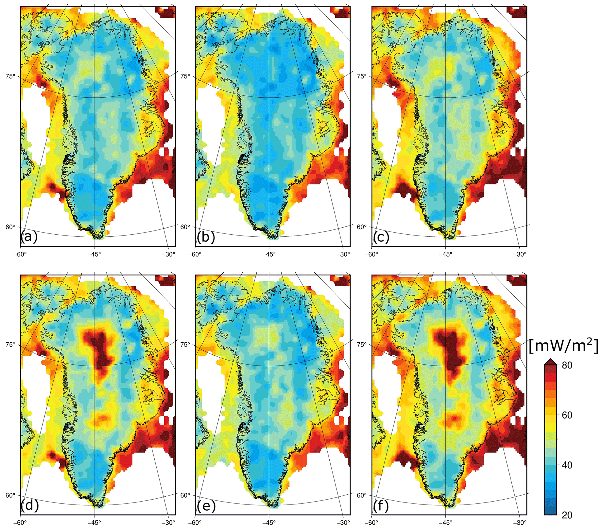
Figure 3Machine learning results highlighting spatial variability due to the jackknifing approach within the continental portion of the domain. The mean (a, d), minimum (b, e), and maximum (c, f) geothermal heat flow calculated from n=59 jackknifing simulations without NGRIP (a, b, c) and n=60 jackknifing simulations with NGRIP (d, e, f).
The jackknifing ensembles suggest that the NGRIP measurement is not representative of the regional background lithospheric heat flow being simulated by the machine learning approach. Simply put, there is no plausible source for high heat flow at NGRIP in the 12 input geophysical datasets provided to the machine learning algorithm (Fig. A1). However, NGRIP and the presence of the Northeast Greenland Ice Stream strongly suggest elevated heat flow in North Greenland. Given appreciable community interest in the NGRIP anomaly, we follow Rezvanbehbahani et al. (2017) and run the machine learning algorithm with training datasets that both include and exclude NGRIP. We make both these “with” and “without” NGRIP heat flow maps available in the database and describe the influence of the NGRIP anomaly on the machine learning approach in Sect. 3.2. Generally, while the location of the NGRIP measurement is unique within Greenland for spatial interpolations, from a machine learning perspective, the relations between observations and geophysical fields are more important than spatial relations. In this sense, our machine learning algorithm does not consider NGRIP a spatial outlier but rather a geophysical outlier; the heat flow at NGRIP is not consistent with other observations of heat flow in similar settings. This suggests that the NGRIP heat flow anomaly is due to local processes that are not captured in the 12 input geophysical datasets.
For the regional overview considered here, precise placement of the continent–ocean transition and type of transitional crust is not critical, so we use the 1000 m bathymetry contour as a simple proxy to delineate oceanic and continental domains. This is a reasonable first-order approximation everywhere except along the Greenland–Iceland Ridge, where the boundary is complex. For the oceanic portion of the domain, where spatial variations in submarine topography and ocean-bottom temperatures influencing heat flow are generally more subtle than on land, we do not employ a jackknife resampling method and instead provide a single heat flow estimate. Although the continental and oceanic simulations were run separately, no edge effects are apparent along the continent–ocean transition.
Figure 4 shows the importance of the individual input variables to the machine learning algorithm for the continental and the oceanic domains of our model. The importance parameter evaluates the relative importance of each input dataset for predicting the results. More details about the calculation and theory of the importance parameter can be found in Lösing and Ebbing (2021). For the continental simulation domain, the distance to volcanoes is the most important feature, followed by the Moho depth and the tectonic regionalization. The mean curvature of the gravity data, the susceptibility model, and the vertical magnetic field component (Bz) are the least important features. For the oceanic simulation domain, the distance to the nearest ridge, the lithosphere–asthenosphere boundary depth, and the tectonic regionalization are the most important features. Differences in feature importance between the continental and oceanic domains support the idea that machine learning can be more precise when each domain is modeled individually. The inclusion or exclusion of NGRIP from the training data does not fundamentally shift this importance ranking of the input geophysical datasets.

Figure 4The importance of the 12 input variables used in the machine learning (a) for the continental model domain and (b) for the oceanic model domain. “Bz” denotes the vertical magnetic field component.
3.1 Heat flow measurement database
The heat flow measurement database presented here contains 290 measurements that are carried forward from IHFC 2018. Eleven of these measurements have been reassessed with new heat flow values (Table 2). The database contains a further 129 measurements that did not appear in IHFC 2018. The majority of these measurements have not been previously published elsewhere. They consist of 88 offshore measurements and 41 onshore measurements, of which 24 are subglacial. Perhaps most notably, these new measurements provide the first comprehensive sampling of heat flow in Davis Strait and Baffin Bay. The mean distance between a new measurement (Type 1) and an existing IHFC 2018 measurement (Type 0) is 251 km, with distance ranging from < 1 km (HF4-9 in Davis Strait) to 645 km (DANA06-HF93_01 in Baffin Bay). The Greenland domain that we employ has an area of 6.4 × 10⁶ km2, which yields a characteristic measurement density of one measurement per ∼ 15 000 km2.
Within the Greenland domain, the median of all heat flow measurements (n=419) is 79 mW m−2, with a standard deviation of 53 mW m−2 (Fig. 5). The highest heat flow measurement is 377 mW m−2 at the RK2105 site on the Mid-Atlantic Ridge just north of Iceland. The lowest heat flow measurement is 3 mW m−2 at the DH-GAP01 site in a permafrost talik in southwestern Greenland. While there is a large range of both onshore and offshore heat flow values, a two-tailed t test, assuming two samples with unequal variance, suggests that the population of offshore heat flows (median 85 mW m−2 and standard deviation 52 mW m−2) is significantly (p < 0.05) warmer than the population of onshore heat flows (mean 58 mW m−2 and standard deviation 55 mW m−2). This difference can be attributed to the more intensively sampled elevated heat flow in the vicinity of the Mid-Atlantic Ridge, in the eastern portion of our Greenland domain. Of the n=419 heat flow measurements, 53 % have a measurement uncertainty of < 5 mW m−2, 40 % have a measurement uncertainty of between 5 and 20 mW m−2, and 7 % have a measurement uncertainty of > 20 mW m−2 (Fig. 6).

Figure 5Histograms of heat flow measurements in the subaerial (n=77), subglacial (n=25), and submarine (n=317) populations (a) and the onshore (n=102) and offshore (n=317) populations (b).
3.2 Greenland heat flow map
Combining multiple simulations from the machine learning algorithm provides a seamless heat flow map across both continental and oceanic areas around Greenland (Fig. 7). This seamless heat flow map represents the mean, or “best estimate”, of geothermal heat flow across the domain. Our “without NGRIP” heat flow simulation suggests a mean onshore heat flow across Greenland of 44 mW m−2, ranging from 28 to 76 mW m−2 across the country. Aside from a heat flow anomaly of up to 100 mW m−2 in central North Greenland, our “with NGRIP” heat flow simulation is broadly similar to the “without NGRIP” simulation. The presence of the NGRIP anomaly, however, increases the mean onshore heat flow across Greenland to 48 mW m−2. Generally, the range between maximum and minimum heat flow simulations is < 20 mW m−2 for most continental areas. The heat flow anomaly around NGRIP is caused by the machine learning algorithm classifying the anomaly region as broadly similar to NGRIP, based on the 12 input geophysical datasets.
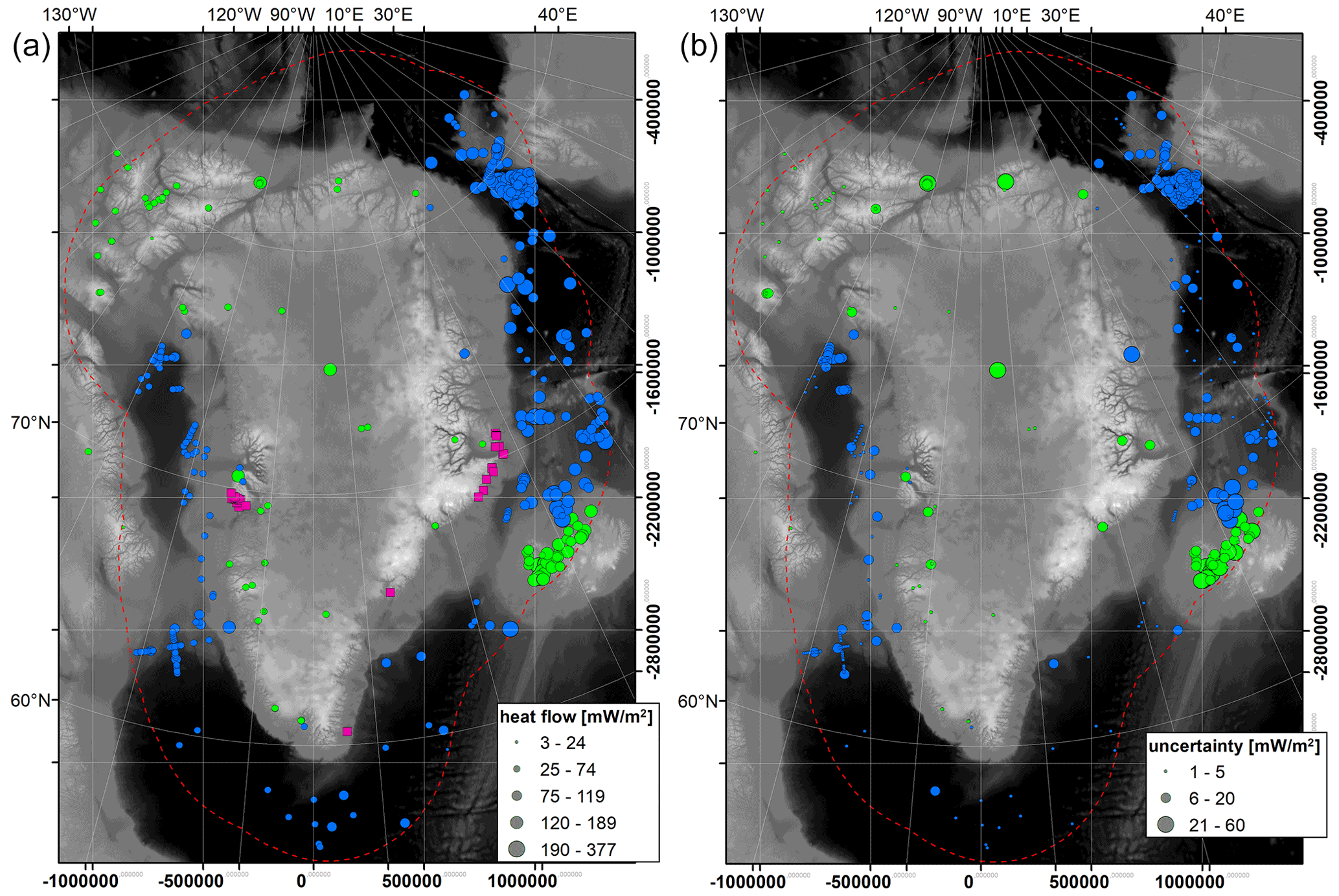
Figure 6(a) Heat flow measurements, scaled by magnitude, overlaid on the ETOPO1 digital elevation model (Amante, and Eakins, 2009). Green dots denote onshore measurements (n=102), and blue dots denote offshore measurements (n=317). Magenta squares denote hot springs inventoried by Hjartarson and Armannsson (2010). (b) The same for uncertainty in heat flow measurement. Projection is EPSG:3413 (bottom x axis and right y axis).
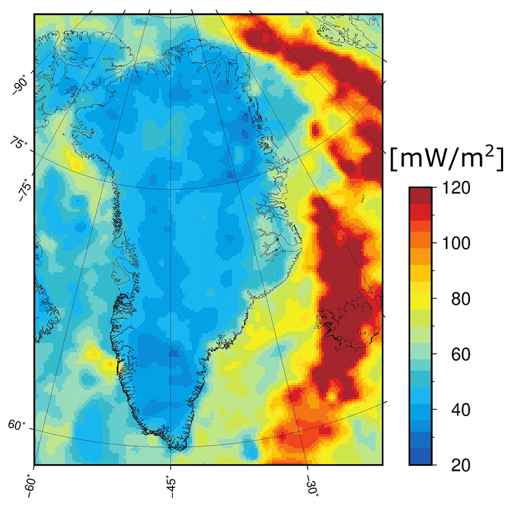
Figure 7Machine learning results for the combined continental and oceanic portions of the domain. For the onshore part, the model trained without NGRIP is used. Note the different color scale in comparison to Fig. 3.
Aside from the NGRIP anomaly, the most distinctive onshore heat flow feature is the relatively low heat flow within the North Atlantic Craton of southern Greenland. As the North Atlantic Craton is an old Archaean block, it is expected to have an average surface heat flow significantly less than younger continental terrains (Goes et al., 2020). Apart from the NGRIP anomaly, the highest onshore heat flow is in east-central Greenland. This positive anomaly, or warm bias, in heat flow is attributable to proximity to the Mid-Atlantic Ridge. Offshore, there is a clear asymmetry to the east and west of Greenland. West of Greenland, in Davis Strait and Baffin Bay, heat flow is generally similar to continental values with some indications of near-shore warm anomalies. However, these warm anomalies may be due to our approximate delineation between continental and oceanic crust types. East of Greenland, in the North Atlantic and Greenland Sea, there is a pronounced high heat flow along the Mid-Atlantic Ridge. Offshore heat flow is enhanced throughout the Irminger Basin off southeastern Greenland.
We compare our modeled heat flow map with the measured heat flow values (Fig. 8). Generally, the residuals between measured and modeled heat flow are < 20 mW m−2 in the continental portion of the domain. NGRIP, however, is a clear outlier in this n=419 site comparison. In the oceanic portion of the domain, the residuals are typically larger. This asymmetry may be attributable to our coarse resolution of the continent–ocean crustal boundary or differences in the accuracy and resolution of geophysical datasets in the onshore and offshore portions of the domain. Our relatively poor delineation of the continent–ocean crustal boundary inevitably results in some oceanic measurements lumped into the continental simulations, and vice versa. These larger residuals suggest that available geophysical datasets do not capture local processes offshore, especially along the Mid-Atlantic Ridge, as well as in some onshore areas. In other words, the global or regional datasets upon which the machine learning algorithm depends have insufficient resolution to capture the variety of local processes reflected in heat flow measurements (Sect. 4.2). This is a fundamental limitation of the 55 km spatial resolution we adopted to ensure a globally consistent heat flow simulation. We expect these residuals to decrease with finer spatial resolution and the inclusion of more geophysical datasets.
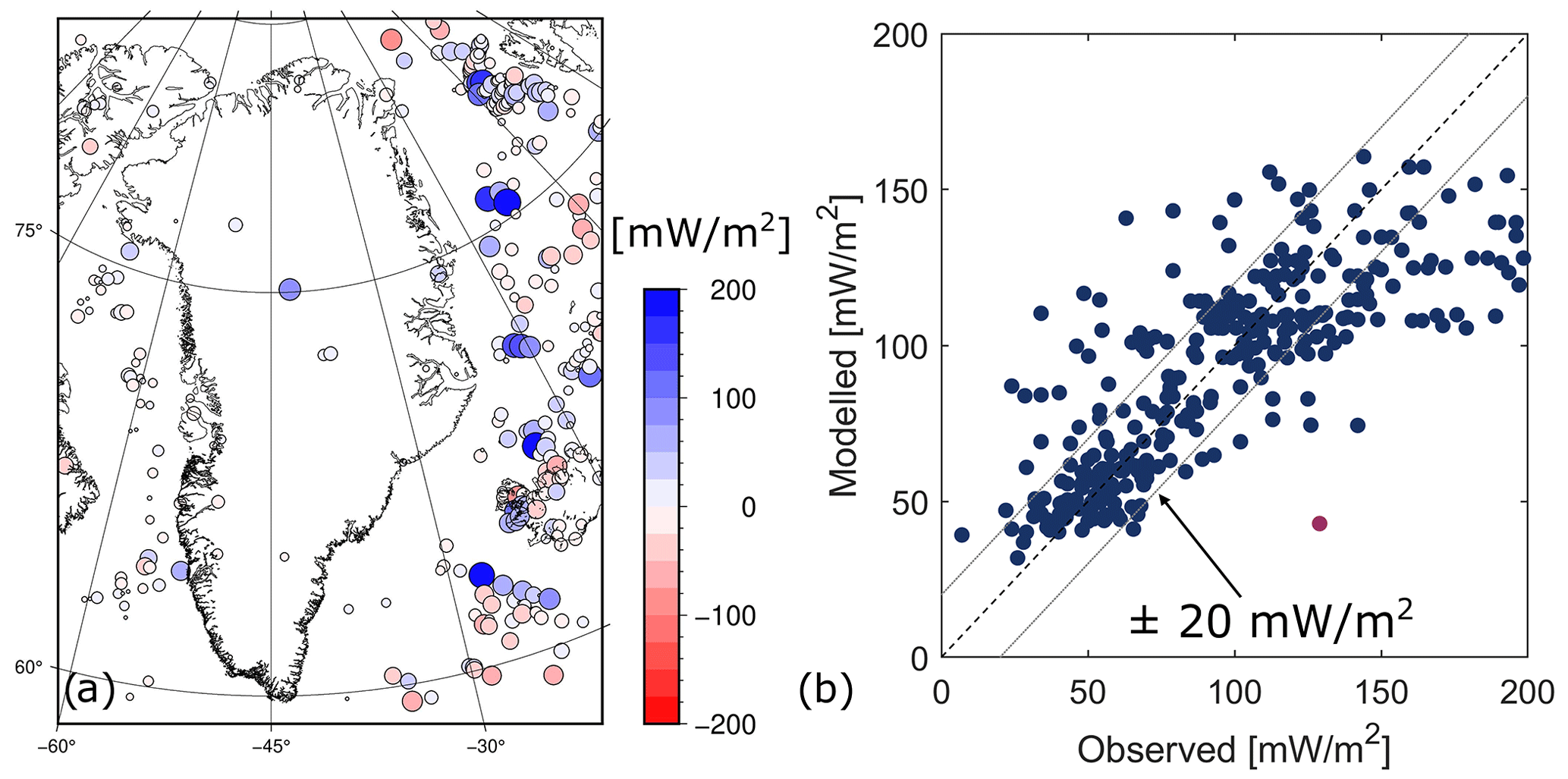
Figure 8(a) Difference (measured minus modeled heat flow) at measurement sites in comparison to our “without NGRIP” simulation. Blues denotes that the model is “colder” than the measurement. (b) Comparison of modeled and observed heat flow values at 419 sites. The NGRIP measurement is included in this comparison as a purple dot.
The magnitude and spatial distribution of heat flow are clearly very sensitive to the inclusion of the relatively high and uncertain NGRIP heat flow measurement (129 ± 30 mW m−2). This machine learning outcome is similar to that highlighted by Rezvanbehbahani et al. (2017). The inclusion of NGRIP in the training data introduces substantial ensemble uncertainty in central North Greenland as the machine learning algorithm cannot reconcile the NGRIP anomaly with available input geophysical datasets. The magnitude and spatial distributions of the ensemble uncertainty ranges of the “with” and “without” NGRIP simulations clearly show that, of all onshore measurements, the machine learning algorithm is most sensitive to the inclusion or exclusion of NGRIP (Fig. 9). Our recommendation to exclude NGRIP from the training data is on the basis that it is not representative of the regional background lithospheric heat flow. The heat flow measured at NGRIP is ∼ 86 mW m−2 greater than the heat flow we simulate at NGRIP: 43 mW m−2, with a range of 35 to 45 mW m−2. However, strictly speaking, the NGRIP ice borehole measurement reflects elevated heat flow in the basal layers of the ice sheet and is not necessarily representative of thermal conditions in the underlying bedrock. A substantial portion of this ∼ 86 mW m−2 discrepancy between observed basal and simulated geothermal heat flows may be attributable to local subglacial hydrological processes (Gooch et al., 2016; Bons et al., 2021; Smith-Johnsen et al., 2021). For example, subglacial water flow or hot springs are much finer-scale processes in comparison to the 55 km resolution of our machine learning algorithm. We note that future additional measurements of elevated heat flows in central North Greenland may yet render NGRIP statistically representative of the broader region. We therefore make both the “with” and “without” NGRIP heat flow maps available in the database.
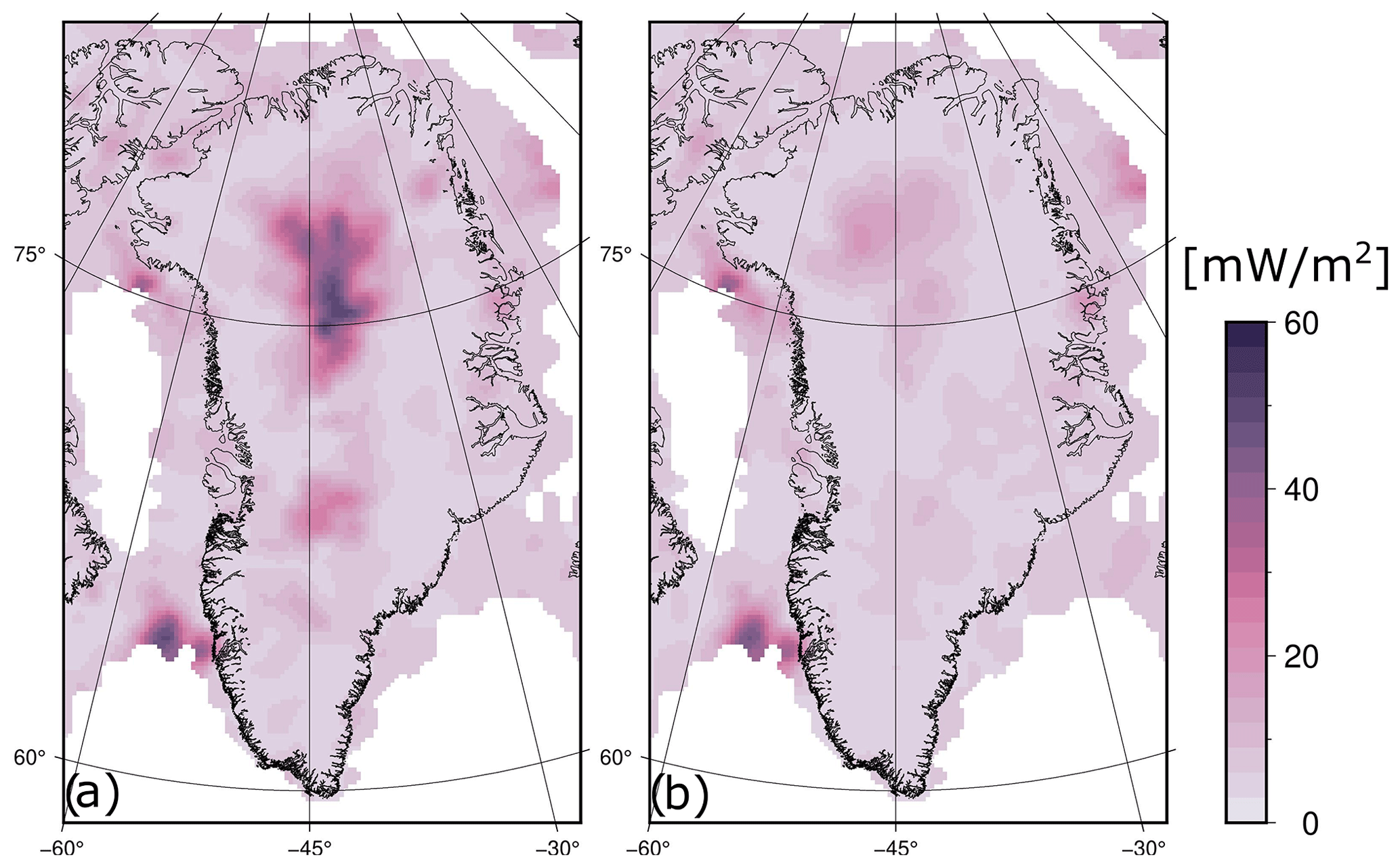
Figure 9The jackknifing ensemble uncertainty range, calculated as the difference between maximum and minimum heat flow, for the (a) “with” and (b) “without” NGRIP simulations. The inclusion of NGRIP introduces substantial ensemble uncertainty in central North Greenland as the machine learning algorithm cannot reconcile the NGRIP anomaly with available input geophysical datasets (Fig. A1).
4.1 Paleoclimate correction
Ground surface temperature is an important boundary condition for geothermal flow. Increases in surface temperature generally decrease the temperature gradient and heat flow, while decreases in surface temperature generally increase the temperature gradient and heat flow. The depth of these heat flow perturbations depends on the magnitude and duration of the paleoclimatic shift. In Arctic settings, the most striking paleoclimatic heat flow perturbations are those associated with submarine-to-subaerial transition. In areas where crustal uplift causes land to emerge from the ocean, geothermal flow is greatly enhanced by the transition from a relatively warm ocean-bottom boundary temperature to a relatively cold atmospheric boundary temperature. While this heat flow anomaly is limited to low-elevation coastal fringes, it can be surprisingly pronounced. For example, a heat flow of 148 mW m−2 was measured in the Alert_203-1 borehole at 5 m elevation, whereas a heat flow of 72 mW m−2 was measured in the Alert_202-2 at 77 m elevation < 2 km away (Taylor et al., 2006). Similarly, the Marraat-1 borehole at 13 m elevation yielded a geothermal flow of 132 mW m−2 (Dam and Christensen, 1994), which is ∼ 160 % greater than the 50 mW m−2 measured at G02_Paakitsoq at higher elevations ∼ 110 km away (Van Tatenhove and Olesen, 1994). While the basalt and gneiss rock types are different between the Marraat-1 and G02_Paakitsoq sites, their thermal properties are not sufficiently different to readily explain this discrepancy in local heat flows.
We demonstrate the magnitude and duration of a submarine-to-subaerial paleoclimate perturbation using a simple 1-D heat flow model. In this model, we prescribe a constant basal heat flow of 50 mW m−2 applied at 500 m depth and uniform thermal diffusivity of 0.5 mm2 s−1. We then assume that the surface boundary condition shifts from a +4 ∘C submarine setting to a −6 ∘C subaerial setting at model initialization. For this submarine-to-subaerial transition, which is characteristic of the Ilulissat area, it is plausible that geothermal flows of > 150 mW m−2 can persist to depths of 100 m for > 400 years as freshly emerged coastal land cools in the atmosphere (Fig. 10). While it is clear that the Alert_203-1 and Marraat-1 boreholes represent encounters with the elevated coastal heat flow anomaly associated with recent land emergence, this effect may influence other heat flow measurements in the database to a lesser degree. Caution should be exercised when interpreting heat flow measurements from land that has emerged in geologically recent times (i.e., since the Little Ice Age). While it may be difficult to interpret anomalous coastal heat flow measurements, it is conceivable that this coastal heat flow anomaly could be harnessed as an indirect, or low-temperature, geothermal heat source for coastal settlements around Greenland.
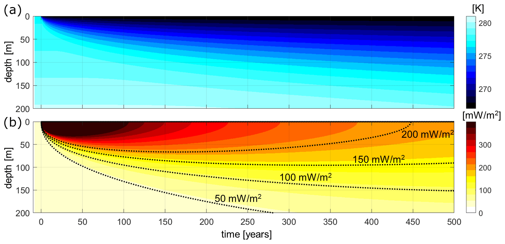
Figure 10Simulation of ground temperature (a) and geothermal flow (b) in response to a change in boundary temperature from submarine to subaerial settings at year 0. This simulation is parameterized to approximate conditions characteristic of Ilulissat, western Greenland.
A second paleoclimatic heat flow perturbation is that associated with subglacial-to-subaerial transitions (and vice versa), as well as transitions between cold-based (or frozen) and warm-based (or thawed) subglacial conditions. The effect of such transitions is highlighted by 2D simulations of bedrock temperature and heat flow at the DH-GAP04 borehole in West Greenland (Claesson Liljedahl et al., 2016; Hartikainen et al., 2021). For this site, an uncorrected heat flow of 28 mW m−2 was calculated over the 280–480 m depth range. The uppermost 280 m of borehole temperatures were discarded to avoid the effect of topography and recent variations in surface climate. Calculation of a longer-term paleoclimatic correction, one that accounts for both ice sheet history and climatic events influencing ground surface temperature, has been performed using a 2D cross-sectional simulation and site-specific data for the past 100 ka (Hartikainen et al., 2021). This period includes a full glacial cycle, during which DH-GAP04 transitioned between ice-covered and ice-free periods, as well as between cold- and warm-based ice sheet conditions. This approach suggests a paleoclimatically corrected heat flow of 38 ± 2 mW m−2, which is ∼ 36 % greater than the present-day measurement. This paleoclimatically corrected heat flow represents the equilibrium heat flow through Earth's crust, unaffected by long-term variations in ground surface temperature over millennial timescales. When interpreting near-surface heat flow in previously glaciated terrain, it is important to use a paleoclimatically corrected heat flow as the deep (or lower) boundary condition, in heat flow simulations.
Figure 11 shows a 2D cross-sectional heat flow simulation at DH-GAP04 that exemplifies both types of glacial transitions described above. First, at around 10 ka (3 kyr before deglaciation), the local basal thermal state of the ice sheet changes from being cold-based (basal ice temperature ∼ −8 ∘C) to warm-based (basal ice temperature at the pressure melting point, ∼ −1 ∘C; Hartikainen et al., 2021). This results in a very strong decrease in heat flow. At the DH-GAP04 borehole, the heat flow is reduced from 35 ± 3 to 12 ± 1 mW m−2 (∼ 65 % decrease). Subsequently, at the time of deglaciation (around 7 ka), the ground surface cools by 2–6 ∘C, compared to the ice-covered warm-based period, as the area becomes subject to Holocene air temperatures. This cooling lithospheric surface boundary condition increases heat flow to 25 ± 5 mW m−2. At this site, the glacial transitions therefore result in complex changes in heat flow, with values ranging from 11 to 38 mW m−2 over the past 100 ka (Hartikainen et al., 2021). Across its 25 km transect distance, this simulation also highlights considerable spatial variability in the heat flow response to glacial transitions. Thus, similar to submarine-to-subaerial transitions, glacial transitions may result in considerable temporal variations in geothermal heat flow with a complex kilometer-scale spatial pattern. Paleoclimatic corrections for previously glaciated terrain will always have some degree of uncertainty associated with assumed basal ice temperature, near-surface ground temperature, and ice cover histories.
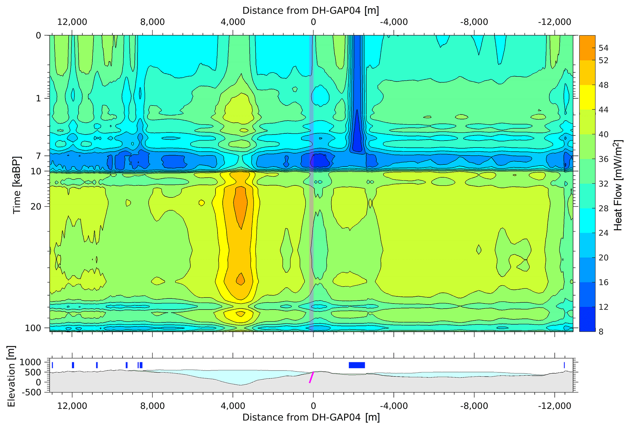
Figure 11Top: simulated temporal changes in ground surface heat flow along a 25 km profile crossing the DH-GAP04 borehole (at a distance of 0 m) during the last glacial cycle (104–0 ka). In this simulation, the ice sheet changed from cold-based to warm-based conditions around 10 ka, and the borehole location was deglaciated around 7 ka. Note the logarithmic scale on the y axis. Bottom: surface topography along the 2D cross-sectional model domain. The DH-GAP04 borehole is shown in pink. Present-day outlet glaciers are shown in light blue, and lake locations are shown by dark-blue bars (Hartikainen et al., 2021).
A third paleoclimatic heat flow consideration is the propagation of surface temperature changes through persistent ice sheet cover to the subglacial interface where heat flow is measured (Calov and Hutter, 1997). The propagation of surface temperatures through the ice sheet is controlled by heat conduction and advection, where the latter is caused by a combination of snowfall leading to vertical transport of relatively cold surface snow downwards and ice flow dynamics giving rise to horizontal ice transport from colder interior sites to warmer marginal sites (Hooke, 2019). In the interior of the ice sheet, advection generally dominates in the upper ice column. There, vertical velocity at the ice sheet surface is effectively equivalent to the snowfall rate, which means that downward advection outpaces upward conduction from the bed. Lower in the ice column, where vertical velocities become smaller, conduction becomes increasingly important. This means that – even in the absence of heat sources or sinks – a deep ice temperature profile measured today is typically not representative of present-day climate but is instead a convolution of competing advection and conduction processes (Calov and Hutter, 1997). Measurements of ice temperatures on the ice divide thus display a cold anomaly in the Last Glacial Period ice temperatures (115–11 ka) and a warm anomaly in the part of the ice column that corresponds in age to the Holocene Climatic Optimum (8–5 ka) (Gundestrup et al., 1994; Dahl-Jensen et al., 2003). Due to conduction, the magnitudes of these anomalies moderate over time. Simply put, however, there can be a multi-centurial to multi-millennial time lag, depending on ice thickness, for surface temperature changes to reach the ice–bed interface at the ice divide. In the ice sheet interior, present-day basal ice temperatures still reflect a past cooler climate, and measured temperature gradient and heat flow will be greater than if Greenland's climate had not changed significantly in the past ca. 100 ka. Indeed, the 61 ± 2 mW m−2 present-day heat flow that we estimate at GRIP is ∼ 20 % greater than the 51 mW m−2 estimated for that site with differing paleoclimatic corrections (Dahl-Jensen et al., 1998; Greve, 2019).
4.2 Other corrections
In addition to correcting local heat flow measurements to account for the effect of non-steady local past climate, there are several other heat flow corrections relevant within the Greenland domain. First, there is local topographic correction to account for elevated heat flow in valleys and correspondingly diminished heat flow along ridge lines (Lees, 1910). This is the only systematic correction currently provided in the database, based on the geostatistical model of Colgan et al. (2021). Within our Greenland domain, this topographic correction ranges from a minimum of −21 ± 5 % at Hole 38 in Ilímaussaq, southern Greenland (Sass et al., 1972), to +55 ± 10 % at the Dybet site in Young Sound, East Greenland (Rysgaard et al., 2018). These end-member sites highlight the potential importance of acknowledging topographic influence on local heat flow. However, there are several measurement sites where topographic correction is not resolved by the Colgan et al. (2021) product, primarily due to geographic limitations. At Agassiz Ice Cap, for example, four borehole ice temperature profiles have been measured within ±1100 m of the same position (Agassiz77, 79A, 79B, and 84; Clarke et al., 1987; Fisher and Koerner, 1994). The ice thicknesses vary between 128 and 341 m across these sites, and assessed heat flows vary between 51 ± 6 and 58 ± 5 mW m−2. Topography likely explains part of the apparent discrepancy among those four closely spaced measurements.
Second, groundwater flow can substantially modify the apparent geothermal heat gradient. The heat advection associated with even relatively small (∼ 1 L s−1) groundwater flows can be comparable to the heat diffusion associated with the geothermal gradient (Mansure and Reiter, 1979). In Greenland, there are clearly some areas where groundwater flow is substantially suppressing or enhancing the apparent geothermal heat gradient. For example, at the DH-GAP01 site near Kangerlussuaq, in southwestern Greenland, the apparent geothermal gradient in a talik beneath a small lake is almost entirely moderated by groundwater flow. There, measured heat flow is reduced by 90 % in comparison to the nearby DH-GAP03 and DH-GAP04 sites (Johansson et al., 2015). In contrast, there are also areas of Greenland with active hot springs where groundwater flow can similarly overwhelm the regional geothermal heat flow value (Persoz et al., 1972). At Unartukavsak, West Greenland, for example, a subaerial 15 ∘C hot spring discharge of 1 L s−1 represents a 63 kW sensible heat source relative to a mean annual air temperature of 0 ∘C (Hjartarson and Armannsson, 2010). This is equivalent to a heat flow of 6300 mW m−2 over a characteristic area of 100 m2. These end-member sites highlight the need to account for the differing influences of “cold” and “hot” groundwater flow onshore, including in subglacial settings.
Third, while approximately half of Earth's contemporary heat flow is ultimately derived from radioactive decay, primarily within the mantle, heat production from near-surface radioactive sources can influence the apparent magnitude and spatial distribution of the deeper geothermal gradient (Lees, 1910). The temperature profiles of the Ilímaussaq boreholes, drilled for the Kvanefjeld uranium prospect in southern Greenland, are substantially influenced by near-surface radioactive heat production. Their measured heat flows (34 to 39 mW m−2) have been estimated to reflect a near-surface radioactive heat production of ∼ 8 µW m−3 over limited horizontal (< 10 km) and vertical (< 1 km) extents. Based on heat flow measurements in analogous Precambrian Shield settings in Canada, Australia, and the United States, Sass et al. (1972) suggested that the measured Ilímaussaq heat flows are 26 % to 44 % higher than the ∼ 27 mW m−2 heat flow that would otherwise be expected for the Precambrian Shield. The Ilímaussaq boreholes highlight the potentially non-trivial influence of near-surface radioactive heat production for altering local geothermal gradients in Greenland. Given the diverse subaerial geology of Greenland and the vast area of poorly resolved subglacial geology beneath the ice sheet (Dawes, 2009), it is likely that there are areas in the Greenland domain beyond Ilímaussaq and Kvanefjeld where heat flow may be similarly influenced by non-trivial heat production associated with near-surface geology.
Finally, lateral contrasts in the thermal conductivity of rock types can result in local heat flow refraction (Jaeger, 1965; Lachenbruch, 1968). In these settings, geotherms close to the geological boundary are influenced by the contrast between relatively high- and low-conductivity rock types, with heat flow diverted from the low-conductivity rock type into the high-conductivity rock type. Sharp spatial contrasts in thermal conductivity associated with rock type may modify local heat flow by ±15 % in subglacial settings (Willcocks et al., 2021). Within our Greenland domain, the effect of lateral conductivity contrasts on heat flow has been qualitatively described at the Isua site. There, Colbeck and Gow (1979) suggest that the heat flow measured in ice sheet boreholes may be biased low as subglacial heat flow is potentially being diverted into the adjacent, and highly conductive, subaerial iron ore formation. With the recent availability of digital maps of subaerial Greenland geology available on open platforms, such as the Escher and Pulvertaft (1995) geological map that now appears in QGreenland (https://qgreenland.org, last access: 8 February 2022), and growing knowledge of variations in thermal conductivity with rock type, it appears feasible to begin systematically quantifying the effect of lateral conductivity contrasts on heat flow across ice-free areas of Greenland.
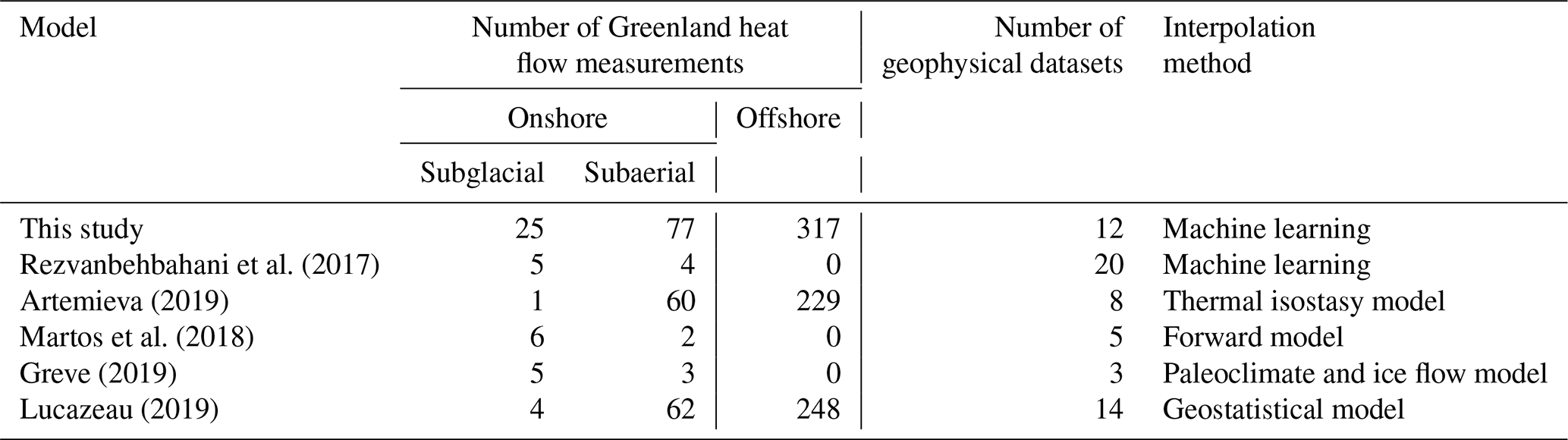
Table 4Number of heat flow observations and geophysical datasets used by this study and five previous studies within the Greenland domain that we consider. These values may be regarded as best estimates. The interpolation method of each study is also listed.
4.3 Comparison of heat flow models
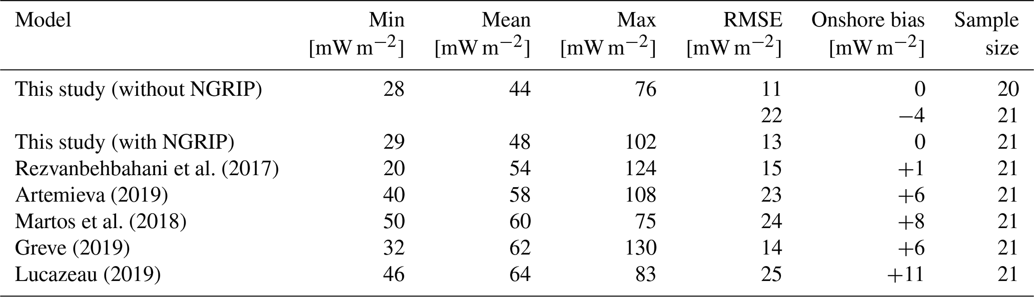
We statistically compare our heat flow model to five previously published Greenland heat flow models, whose inputs and methods are summarized and compared with ours in Table 4. With a mean Greenland heat flow of 44 mW m−2, our “without NGRIP” simulation infers the lowest mean Greenland heat flow across all models to date (Table 5). Even when including NGRIP in the continental jackknifing simulations, our mean “with NGRIP” heat flow only increases to 48 mW m−2. When comparing all seven heat flow simulations with the n=21 grid cells of binned heat flow measurements (including NGRIP) within the Greenland land area common to all seven models, we find that our model, which includes NGRIP in the training dataset, has the smallest bias and root mean square error (RMSE). Our model is followed by the model of Rezvanbehbahani et al. (2017), which has the second-smallest bias, and the model of Greve (2019), which has the second-lowest RMSE (Fig. 12). If we exclude the NGRIP measurement from the comparison our simulation trained without NGRIP yields the smallest bias (0 mW m−2) and RMSE (11 mW m−2). As we exclude the relatively high and uncertain NGRIP heat flow measurement from our training dataset, our model clearly does not reproduce this heat flow anomaly, unlike models that do include the NGRIP measurement. However, even our model that is trained with NGRIP predicts a heat flow value of only 90 mW m−2 at NGRIP, which is 39 mW m−2 less than the measured value (129 mW m−2). This difference of 39 mW m−2 between measured and predicted values remains the highest residual among all onshore sites (Fig. 12).
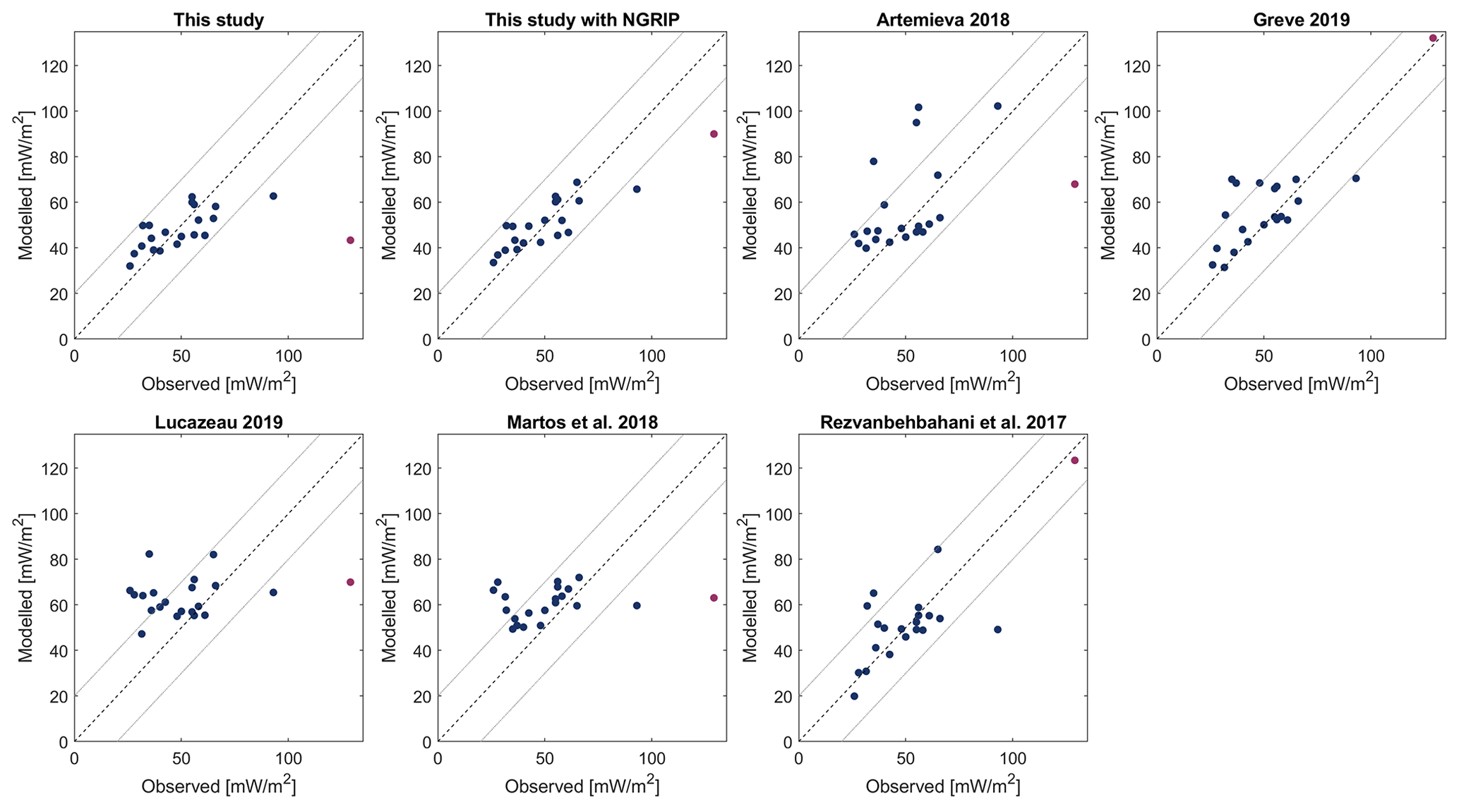
Figure 12Comparison of simulated and measured geothermal heat flow in binned 55 km grid cells within the Greenland land area common to all seven models (n=21; Table 4). RMSE and bias for each model listed in Table 5. The NGRIP measurement is included in this comparison as a purple dot.
We also qualitatively compare the magnitude and spatial distribution of our geothermal heat flow map without NGRIP with these five previous studies (Fig. 13). In comparison to the most methodologically similar model, the machine learning model of Rezvanbehbahani et al. (2017), we infer a significantly cooler central North Greenland. This pronounced difference can be explained partly by our choice of excluding the NGRIP measurement, but also the model which is trained with NGRIP is colder in central North Greenland than Rezvanbehbahani et al. (2017). We also employed more Greenland regional datasets, which are generally finer-resolution and better suited to our study area than global datasets, and trained our model with a significantly larger number of in situ measurements.
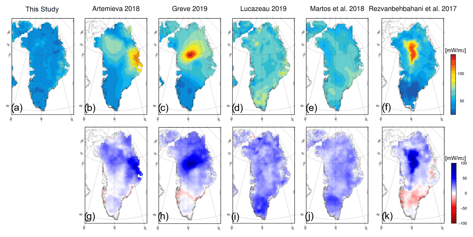
Figure 13Comparison of the heat flow model of this study without NGRIP (a) to previously published models: (b) thermal isostasy from Artemieva (2019) model 1, (c) fitting to available heat flow data from Greve (2019), (d) global similarity study from Lucazeau (2019), (e) magnetic data from Martos et al. (2018), and (f) machine learning by Rezvanbehbahani et al. (2017) with NGRIP = 135 mW m−2. Anomaly plots are shown in (g) to (k), where blue denotes this study as “colder”. Mean geothermal heat flow of each model summarized in Table 6.
The Lucazeau (2019) heat flow model is also geostatistical as it relies on empirical correlations between global geophysical datasets and heat flow measurements. While the Lucazeau (2019) model shares similar length scales of spatial variability (∼ 50 km), its patterns are quite different from our model. For example, they infer a relatively warm North Atlantic Craton. These differences can be attributed to our explicit preference for more detailed regional datasets instead of global datasets where possible. An additional source of deviation from the Lucazeau (2019) model may be their manual weighting of included geophysical datasets, whereas our machine learning algorithm includes geophysical datasets without a priori weights.
Martos et al. (2018) based their heat flow model on identifying deep magnetic sources, assuming that the deepest sources coincide with the Curie isotherm and constructing a regional thermal model of heat flow. Their regional thermal model infers a band of enhanced heat flow anomaly from central East Greenland to northwestern Greenland. Our model does not infer this enhanced heat flow anomaly and also finds substantially lower heat flows in the North Atlantic Craton. We attribute these differences to the choice of input data, including availability of heat flow measurements and differing geostatistical and thermal modeling approaches.
Artemieva (2019) proposed a thermal isostasy method to calculate upper-mantle temperatures, lithosphere thickness, and geothermal heat flow using bedrock topography, ice thickness, and Moho depth from seismic data. This approach is sensitive to the choice of surface-wave-tomography models and reference values. Our model has the largest discrepancy with the Artemieva (2019) model along the coast of central East Greenland, where our model infers a substantially lower heat flow over a broad region. All four other models, however, also predict lower heat flows than Artemieva (2019) in this region, which suggests that this anomaly is unique to the data or methodology of Artemieva (2019).
Finally, the Greve (2019) heat flow model uses a numerical ice sheet model to infer the heat flow required to match observed basal ice temperatures at ice core locations, treating the Pollack et al. (1993) heat flow model as an a priori guess. Similar to the difference field with Rezvanbehbahani et al. (2017), our difference field with Greve (2019) highlights the NGRIP measurement site, where we predict a much lower regional heat flow. The spatial patterns in the Greve (2019) model suggest it is sensitive to a relatively small number of input heat flow measurements (n=8). Part of the difference from our model may therefore be attributable to differing availability of heat flow measurements between studies.
Table 5Minimum, mean, and maximum heat flow over Greenland onshore area from this study and five previous studies. Root mean square error (RMSE) and simulated minus measured bias relative to heat flow measurements within the common land area domain also shown (Fig. 12). Here, the number of onshore heat flow measurements (sample) reflects binned 55 km grid cells. See Table 4 for a comparison of the heat flow measurements used in each of these studies.
4.4 Icelandic plume track
There is substantial interest in understanding the paleo-Icelandic plume track beneath Greenland and its ice sheet. Generally, there is consensus among plume track models that the Icelandic plume was located in the vicinity of present-day Kangersertuaq Fjord in central East Greenland at ∼ 50 Ma (Morgen, 1983; Forsyth et al., 1986; Müller et al., 1993; Doubrovine et al., 2012; Martos et al., 2018). In addition to reconstructing past tectonic motion, this paleoplume fix is supported by the presence of basalts up to 7 km thick from the North Atlantic Igneous Province dated to ∼ 56 Ma along the Blosseville Coast (Storey et al., 2007) and the presence of a relatively low upper-mantle viscosity there today (Khan et al., 2016). However, there is less consensus as to the plume position prior to this time, with analogous west coast plume positions previously hypothesized from Disko Island (70∘ N) to Petermann Glacier (81∘ N). It has also been recently suggested that Greenland bears the imprint of not just one, but two plume tracks with differing histories of activity (Toyokuni et al., 2020).
Our model does not show an area of elevated heat flow that might be interpreted as a remnant of the Icelandic plume track. This pattern is consistent with Rezvanbehbahani et al. (2017), Greve (2019), and Lucazeau (2019) but differs from Martos et al. (2018) and Artemieva (2019), which both infer plume tracks. An earlier model from Rogozhina et al. (2016) can also be interpreted in terms of west-to-east passage of a plume. There is debate over the potential influence of paleoplume activity on present-day heat flow beneath the Greenland Ice Sheet (Smith-Johnsen et al., 2020; Bons et al., 2021). It is plausible that enhanced heat flow of ∼ 10 mW m−2 may exist along the most recent 50 Ma of the plume track, but heat flow anomalies likely become difficult to observe after this time as heat flow returns to balance (Martos et al., 2018). The main observable impacts of paleoplume activity are now likely limited to the base of the lithosphere, meaning that plume tracks derived from geophysical modeling may not reflect near-surface heat flow but rather an imprint of underlying lithospheric architecture.
Interpretations of paleoplume tracks are further complicated by the presence of very young volcanic and geothermal processes. Young igneous formations in East Greenland, dated to 14 Ma, suggest very recent widespread volcanism well after Greenland moved off the Icelandic plume (Storey et al., 2004). Similarly, the presence of coastal geothermal hot springs in both central West and central East Greenland suggests appreciable contemporary heat sources far from the contemporary location of the Icelandic plume (Hjartarson and Armannsson, 2010; Fig. 6). Storey et al. (2004) suggested that metasomatic processes and emplacement of volatiles from the plume into the shallow mantle may have had long-lived influence on the region. It is conceivable that small pressure perturbations resulting from loading and unloading of ice sheets and/or tectonic stresses could result in local volcanism in such a mantle (Jull and McKenzie, 1996). A north–south transect of onshore heat flow measurements in central East Greenland, either subaerial, subglacial, or a combination of both, could improve understanding of the residual heat flow anomaly associated with the paleoplume as well as offer insight on elevated heat flow potential associated with young secondary processes.
Digital assets for the Greenland Geothermal Heat Flow Database and Map (Version 1) are now available open-access on the GEUS Dataverse at https://doi.org/10.22008/FK2/F9P03L (Colgan and Wansing, 2021). These include (1) heat flow measurement database as .xlsx and .shp, (2) heat flow maps at 10 and 55 km resolutions as .xyz and .nc for the model with and without NGRIP, (3) hot spring database as .xlsx, (4) regional coast+500 km domain boundary as .shp, and (5) extrapolation code for subglacial temperature gradients as .m. The primary temperature and stratigraphy profiles of the Hellefisk-1, Ikermiut-1, Kangâmiut-1, Nukik-1/2, Alpha-1, Atammik2-1 (AT2-1), Atammik7-1 (AT7-1), Delta-1, Gamma-1, LadyFranklin7-1 (LF7-1), Qulleq-1, T4-1, and T8-1 submarine boreholes are owned by the Geological Survey of Denmark and Greenland. The derived temperature gradients and heat flows included here are published with special permission. The primary temperature and stratigraphy profiles of the Alcoa_Site7e-I, Alcoa_Site7e-P, and Alcoa_Site6g-P subaerial boreholes are jointly owned by the Greenland Government and Alcoa. The derived temperature gradients and heat flows included here are published with special permission.
Here, we document the first version of the Greenland Geothermal Heat Flow Database and Map. While we have increased the available heat flow measurements by 44 % (290 to 419) within the Greenland domain, onshore measurements remain disproportionately scarce. Greenland represents ∼ 1.5 % of global land area, but – once our regional database is merged into the IHFC database – Greenland will only represent 0.08 % of IHFC onshore measurements. We anticipate updating this measurement database as new measurements and corrections become available. We will continue efforts to parse the Type 2 sites (uncertain temperature data) into either Type 1 (new measurement) or Type 3 (no temperature data) classes. Topographic correction is presently the only systematic correction available within the measurement database, but there is clearly a need for more systematic corrections. Most notably, the application of a standardized, yet site-specific paleoclimatic correction to all measurement sites would ensure that heat flow measurements are interpreted in the correct climatic context.
We have used machine learning to create a heat flow map that is self-consistent with this measurement database. While there has been a proliferation of Greenland heat flow maps in the past decade, compilations of in situ heat flow measurements have generally lagged these models. The heat flow map we present may be the first of a new generation of heat flow maps that are self-consistent with a larger and better documented inventory of in situ heat flow measurements. Clearly, a fundamental question in mapping Greenland heat flow is whether or not to include NGRIP as a regionally representative heat flow measurement. This touches on a larger issue of how to not only understand the effect of local processes in measurements but also how to represent the influence of these local processes in large-scale models. For the NGRIP measurement, this may mean resolving potential differences between “basal” and “geothermal” heat flows. In regional models, this may mean representing the cumulative effect of local processes like widespread hot spring activity.
There is a present possibility of using unconventional sources to increase the inventory of available in situ Greenland heat flow measurements. Abandoned prospecting wells can be repurposed for heat flow measurements by inserting temperature strings to measure local geothermal gradients. While this requires knowledge of well closure and present conditions, it has been successful in the past. Local temperature gradients can also be resolved by combining knowledge of seismic- or radar-derived permafrost depth with mean annual ground temperature. This is most feasible in valley bottoms, where the permafrost is contained within a thick sediment package, and there is free water below the permafrost limit. Finally, while hot spring temperatures do not serve as reliable indicators of regional geothermal heat flow, chemical analyses of their water can resolve deep temperatures that are characteristic of regional phenomena and heat flow. It is likely that many uncharted hot springs – both subaerial and subglacial – exist in Greenland.
There are presently at least four grand challenges that motivate further improvement of our scientific understanding of Greenland's geothermal heat flow. First, geothermal heat flow is a critical basal boundary condition for the thermomechanical ice flow models being used to project Greenland's future sea level rise contribution. Second, geothermal heat flow is similarly a critical basal boundary condition influencing the stability of periglacial processes and landforms, including both onshore permafrost and shallow offshore gas hydrates, that can deteriorate under future climate change. Third, resolving how the present-day magnitude and spatial distribution of geothermal heat flow may reflect the pre-50 Ma influence of the Icelandic plume track may be key to resolving Greenland's geologic history. Finally, from a social perspective, there appears to be potential for low-temperature geothermal heating to play a role in Greenland's green-energy transition.
Table A1Comparison of the data fields in the IHFC 1976 and 2021 database structures (Jessop et al., 1976; Fuchs et al., 2021a) and this study. “X” denotes an included field. Red outlines and bold text denote the 18 mandatory data fields of the IHFC 2021 structure, and red shading denotes the 8 mandatory data fields that are not available in our new database. Here, “T” denotes temperature, and “TC” denotes thermal conductivity. Full IHFC naming convention described in Fuchs et al. (2021a).

Table A2Geophysical datasets and features provided to the machine learning algorithm to spatially interpret point measurements of heat flow. Data extent is global unless otherwise stated. A graphical overview of these input datasets is shown in Fig. A1.

n/a – not available
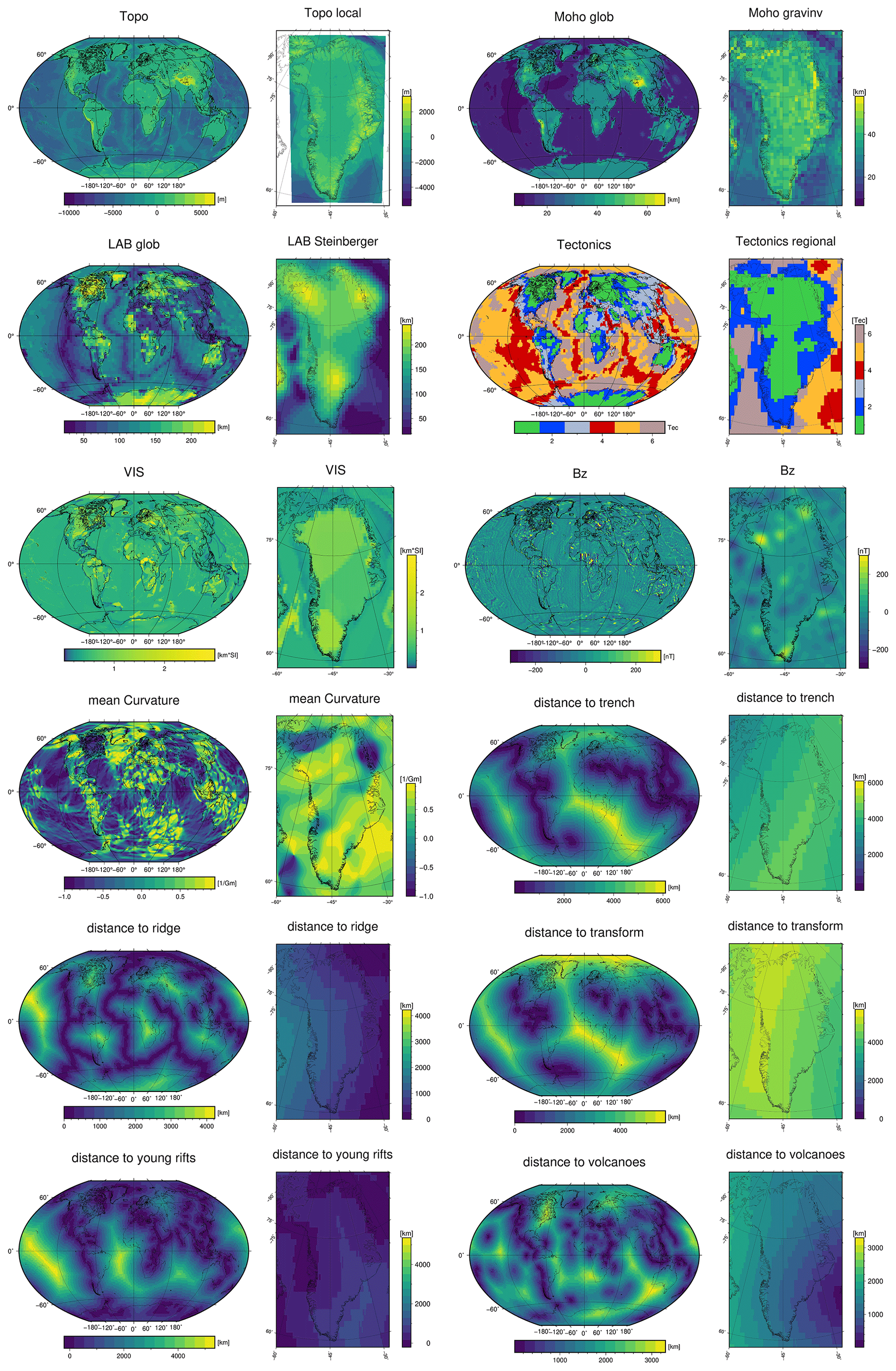
Figure A1Graphical overview of the 12 geophysical datasets and features provided to the machine learning algorithm (Table A2). Each variable is shown in both global and local (Greenland) extents.
Author contribution is captured following the CRediT system. Conceptualization by WC, AG, KM, RSF, AB. Data curation by KM, KL, FGC, TIN, LCL, AH, SB, SF, JH, JL, DDJ, JON, NB, TF, DP, UG, GD, TN. Formal analysis by WC, AG, ML, KL, JE, FGC, TIN, LCL, DDJ, FM, TF. Funding acquisition by WC, JE, RSF. Investigation by WC, AG, KM, JH, JE, TIN, JAM, NBK, RSF, AB, FM, YM, KKK. Interpretation by WC, AG, KM, ML, JH, JE, FGC, LCL, JAM, AH, SB, NBK, JH, JL, DDJ, AB, JON, FM, YM, KKK, SAK, AL. Methodology by WC, AG, KM, ML, JE, SF, DDJ, KKK. Project administration by WC, AG, KM, RSF. Software: WC, AG, ML, JE. Supervision by WC, JE, SAK. Validation by WC, AG, ML, JE. Visualization by WC, AG, JH. Writing (pre-submission) by WC, AG, KM, ML, JH, JE, LCL, JAM, NBK, SF, JH, JL, JON, YM, KKK, AL. Writing (revisions) by WC, AG, JAM.
The contact author has declared that neither they nor their co-authors have any competing interests.
Publisher's note: Copernicus Publications remains neutral with regard to jurisdictional claims in published maps and institutional affiliations.
The authors thank Ralf Greve (Hokkaido University) and the anonymous referee for their helpful reviews of this work as well as Kirsten Elger (German Research Centre for Geosciences) for serving as scientific editor.
This publication is made possible by the award “HOTROD: Prototype for Rapid Sampling of Ice-Sheet Basal Temperatures” supported by the Experiment Programme of the Villum Foundation (grant no. 00022885). This work has also been supported by the Programme for Monitoring of the Greenland Ice Sheet (http://www.promice.dk, last access: 8 February 2022), funded by the Danish Ministry of Climate, Energy and Utilities. Additional support was given by the European Space Agency through the STSE 3D Earth and the German Research Council (DFG) to the projects “GreenCrust” and “Antarctic Heat”, the latter in the framework of the priority program SPP 1158: Antarctic Research with Comparable Investigations in Arctic Sea Ice Areas. Observational and modeled data for the DH-GAP04 drill hole were financed by the Swedish Nuclear Fuel and Waste Management Company (SKB).
This paper was edited by Kirsten Elger and reviewed by Ralf Greve and one anonymous referee
Afonso, J., Salajegheh, F., Szwillus, W., Ebbing, J., and Carmen, C.: A global reference model of the lithosphere and upper mantle from joint inversion and analysis of multiple data sets, Geophys. J. Int., 217, 1602–1628, https://doi.org/10.1093/gji/ggz094. 2019.
Amante, C. and Eakins, B.: ETOPO1 1 Arc-Minute Global Relief Model: Procedures, Data Sources and Analysis, Technical Memorandum NESDIS NGDC-24, National Geophysical Data Center [data set], NOAA, https://doi.org/10.7289/V5C8276M, 2009.
Artemieva, I.: Lithosphere structure in Europe from thermal isostasy, Earth-Sci. Rev., 188, 454–468, https://doi.org/10.1016/j.earscirev.2018.11.004, 2019.
Balling, N. and Brooks, C.: Heat Flow Measurements in the Skaregaard Intrusion: A Progress Report, Kangerdlugssuaq Studies, Proceedings of a meeting held on January 1991 in the Geological Institute, University of Copenhagen, 1991.
Beltrami, H. and Mareschal, J.-C.: Recent warming in eastern Canada inferred from geothermal measurements, Geophys. Res. Lett., 18, 605–608, https://doi.org/10.1029/91GL00815, 1991.
Bjerager, M., Piasecki, S., and Bojesen-Koefoed, J.: The Upper Jurassic Blokelv-1 cored borehole in Jameson Land, East Greenland – an introduction, GEUS Bulletin, 42, 7–14, https://doi.org/10.34194/geusb.v42.4307, 2018.
Bliss, A.: Polar stereographic coordinate transformation (lat/lon to map), MATLAB Central File Exchange, https://www.mathworks.com/matlabcentral/fileexchange/32950-polar-stereographic-coordinate-transformation-lat-lon-to-map (last access: 27 April 2022), 2021.
Bons, P. D., de Riese, T., Franke, S., Llorens, M.-G., Sachau, T., Stoll, N., Weikusat, I., Westhoff, J., and Zhang, Y.: Comment on “Exceptionally high heat flux needed to sustain the Northeast Greenland Ice Stream” by Smith-Johnsen et al. (2020), The Cryosphere, 15, 2251–2254, https://doi.org/10.5194/tc-15-2251-2021, 2021.
Buchardt, S. and Dahl-Jensen, D.: Estimating the basal melt rate at NorthGRIP using a Monte Carlo technique, Ann. Glaciol., 45, 137–142, https://doi.org/10.3189/172756407782282435, 2007.
Calov, R. and Hutter, K.: Large scale motion and temperature distributions in land-based ice shields; the Greenland Ice Sheet in response to various climatic scenarios, Archives Mech., 49, 919–962, 1997.
Celli, N., Lebedev, S., Schaeffer, A., and Gaina, C.: The tilted Iceland Plume and its effect on the North Atlantic evolution and magmatism, Earth Planet. Sc. Lett., 569, 117048, https://doi.org/10.1016/j.epsl.2021.117048, 2021.
Claesson Liljedahl, L., Lehtinen, A., Harper, J., Näslund, J.-O., Selroos, J.-O., Pitkänen, P., Puigdomenech, I., Hobbs, M., Follin, S., Hirschorn, S., Jansson, P., Järvinen, H., Kennell, L., Marcos, N., Ruskeeniemi, T., Tullborg, E.-L., and Vidstrand, P.: Greenland Analogue Project: Final Report, SKB Report TR-14-13. Svensk Kärnbränslehantering AB, 2016.
Clarke, G., Fisher, D., and Waddington, W.: Wind pumping: A potentially significant heat source in ice sheets, The Physical Basis of Ice Sheet Modelling, IAHS Publication Number 170, 169–180, 1987.
Classen, D: Temperature Profiles for the Barnes Ice Cap Surge Zone, J. Glaciol., 18, 391–405, https://doi.org/10.3189/S0022143000021079, 1977.
Clausen, H., Stampe, M., Hammer, C., Hvidberg, C., Dahl-Jensen, D., and Steffensen, J. P.: Glaciological and chemical studies on ice cores from Hans Tausen ice cap, Greenland, Meddelelser om Grønland, 39, 123–149, 2001.
Colbeck, S. and Gow, A.: The margin of the Greenland Ice Sheet at Isua, J. Glaciol., 24, 155–165, https://doi.org/10.3189/S0022143000014714, 1979.
Colgan, W. and Wansing, A.: Greenland Geothermal Heat Flow Database and Map, GEUS DataVerse [data set], https://doi.org/10.22008/FK2/F9P03L, 2021.
Colgan, W., MacGregor, J., Mankoff, K., Haagenson, R., Rajaram, H., Martos, Y., Morlighem, M., Fahnestock, M., and Kjeldsen, K.: Topographic Correction of Geothermal Heat Flux in Greenland and Antarctica, J. Geophys. Res., 126, e2020JF005598, https://doi.org/10.1029/2020JF005598, 2021.
Cox, D., Huuse, M., Newton, A., Sarkar, A., and Knutz, P.: Shallow gas and gas hydrate occurrences on the northwest Greenland shelf margin, Mar. Geol., 432, 106382, https://doi.org/10.1016/j.margeo.2020.106382, 2021.
Dahl-Jensen, D., Mosegaard, K., Gundestrup, N., Clow, G., Johnsen, S., Hansen, A., and Balling, N.: Past Temperatures Directly from the Greenland Ice Sheet, Science, 282, 268–271, https://doi.org/10.1126/science.282.5387.268, 1998.
Dahl-Jensen, D., Gundestrup, N., Gogineni, S., and Miller, H.: Basal melt at NorthGRIP modeled from borehole, ice-core and radio-echo sounder observations, Ann. Glaciol., 37, 207–212, https://doi.org/10.3189/172756403781815492, 2003.
Dam, G. and Christiansen, F.: Well summary Marraat-1, Nuussuaq, West Greenland, Open File Series, GGU Report, 94/11, 1994.
Damm, V: The expedition of the Research Vessel “Polarstern” to the Arctic in 2010 (ARK-XXV/3), Alfred Wegener Institute, https://doi.org/10.2312/BzPM_0621_2010, 2010.
Davies, W., Krinsley, D., and Nicol, A.: Geology of the North Star Bugt area, Northwest Greenland, Meddeleser om Grønland, 162, 1–68, 1963.
Davis, R.: Approach Roads, Greenland, 1960–1964, Cold Regions and Research and Engineering Laboratory, Technical Report 133, 1967.
Dawes, P.: The bedrock geology under the Inland Ice: the next major challenge for Greenland mapping, GEUS Bulletin, 17, 57–60, https://doi.org/10.34194/geusb.v17.5014, 2009.
Doubrovine, P., Steinberger, B., and Torsvik, T.: Absolute plate motions in a reference frame defined by moving hotspots in the Pacific, Atlantic and Indian oceans, J. Geophys. Res., 117, B09101, https://doi.org/10.1029/2011JB009072, 2012.
Doyle, S., Hubbard, B., Christoffersen, P., Young, T., Hofstede, C., Bougamont, M., Box, J., and Hubbard, A.: Physical Conditions of Fast Glacier Flow: 1. Measurements From Boreholes Drilled to the Bed of Store Glacier, West Greenland, J. Geophys. Res., 123, 324–348, https://doi.org/10.1002/2017JF004529, 2018.
Ebbing, J., Haas, P., Ferraccioli, F., Pappa, F., Szwillus, W., and Bouman, J.: Earth tectonics as seen by GOCE – Enhanced satellite gravity gradient imaging, Sc. Rep., 8, 16356, https://doi.org/10.1038/s41598-018-34733-9, 2018.
Ebbing, J., Dilixiati, Y., Haas, P., Ferraccioli, F., and Scheiber-Enslin, S.: East Antarctica magnetically linked to its ancient neighbours in Gondwana, Sci. Rep., 11, 5513, https://doi.org/10.1038/s41598-021-84834-1, 2021.
Escher, J. and Pulvertaft, T.: Geological map of Greenland. 1:2,500,000, Copenhagen, Geological Survey of Denmark and Greenland, 1995.
Fisher, D. and Koerner, R.: Signal and noise in four ice-core records from the Agassiz Ice Cap, Ellesmere Island, Canada: Details of the last millennium for stable isotopes, melt and solid conductivity, Holocene, 4, 113–120, https://doi.org/10.1177/095968369400400201, 1994.
Fisher, D., Koerner, R., Bourgeois, J., Zielinski, G., Wake, C., Hammer, C., Clausen, H., Gundestrup, N., Johnsen, S., Goto-Azuma, K., Hondoh, T., Blake, E., and Gerasimoff, M.: Penny Ice Cap Cores, Baffin Island, Canada, and the Wisconsinan Foxe Dome Connection: Two States of Hudson Bay Ice Cover, Science, 279, 692–695, https://doi.org/10.1126/science.279.5351.692, 1998.
Forsyth, D., Morel-a-l'Huissier, P., Asudeh, I., and Green, A.: Alpha ridge and Iceland-products of the same plume?, J. Geodynam., 6, 197–214, https://doi.org/10.1016/0264-3707(86)90039-6, 1986.
Fuchs, S., Beardsmore, G., Chiozzi, P., Gola, G., Gosnold, W., Harris, R., Jennings, S., Liu, S., Negrete-Aranda, R., Neumann, F., Norden, B., Poort, J., Rajver, D., Ray, L., Richards, M., Smith, J., Tanaka, A., and Verdoya, M.: A new database structure for the IHFC Global Heat Flow Database, International Journal of Terrestrial Heat Flow and Applied Geothermics, 22, 1–4, https://doi.org/10.31214/ijthfa.v4i1.62, 2021a.
Fuchs, S., Norden, B. and International Heat Flow Commission: The Global Heat Flow Database: Release 2021, GFZ Data Services, https://doi.org/10.5880/fidgeo.2021.014, 2021b.
Global Heat Flow Compilation Group: Component parts of the World Heat Flow Data Collection, PANGAEA [data set], https://doi.org/10.1594/PANGAEA.810104, 2013.
Goes, S., Hasterok, D., Schutt, D., and Klöcking, M.: Continental lithospheric temperatures: A review, Phys. Earth Planet. In., 306, 106509, https://doi.org/10.1016/j.pepi.2020.106509, 2020.
Gooch, B., Young, D. and Blankenship, D.: Potential groundwater and heterogeneous heat source contributions to ice sheet dynamics in critical submarine basins of East Antarctica, Geochem. Geophy. Geosy., 17, 395–409, https://doi.org/10.1002/2015GC006117, 2016.
Goutorbe, B., Poort, J., Lucazeau, F., and Raillard, S.: Global heat flow trends resolved from multiple geological and geophysical proxies, Geophys. J. Int., 187, 1405–1419, https://doi.org/10.1111/j.1365-246X.2011.05228.x, 2011.
Greve, R.: Relation of measured basal temperatures and the spatial distribution of the geothermal heat flux for the Greenland ice sheet, Ann. Glaciol., 42, 424–432, https://doi.org/10.3189/172756405781812510, 2005.
Greve, R.: Geothermal heat flux distribution for the Greenland ice sheet, derived by combining a global representation and information from deep ice cores, Polar Data J., 3, 22–36, https://doi.org/10.20575/00000006, 2019.
Gundestrup, N. and Hansen, B.: Bore-Hole Survey at Dye 3, South Greenland, J. Glaciol., 30, 282–288, https://doi.org/10.3189/S0022143000006109, 1984.
Gundestrup, N., Clausen, H., and Hansen, B.: The UCPH bore-hole logger, National Institute for Polar Research, Special Issue, 49, 224–233, 1994.
Haas, P., Ebbing, J., and Szwillus, W.: Sensitivity analysis of gravity gradient inversion of the Moho depth – a case example for the Amazonian Craton, Geophys. J. Int., 221, 1896–1912, https://doi.org/10.1093/gji/ggaa122, 2020.
Hansen, B. and Langway, C.: Deep core drilling in ice and core analysis at Camp Century, Greenland, 1961–1966, Antarct. J. USA, 1, 207–208, 1966.
Hansson, M.: The Renland ice core. A Northern Hemisphere record of aerosol composition over 120,000 years, Tellus B, 46, 390–418, https://doi.org/10.3402/tellusb.v46i5.15813, 1994.
Harper, J., Hubbard, A., Ruskeeniemi, T., Claesson Liljedahl, L., Lehtinen, A., Booth, A., Brinkerhoff, D., Drake, H., Dow, C., Doyle, S., Engström, J., Fitzpatrick, A., Frape, S., Henkemans, E., Humphrey, N., Johnson, J., Jones, G., Joughin, I., Klint, K., Kukkonen, I., Kulessa, B., Landowski, C., Lindbäck, K., Makahnouk, M., Meierbachtol, T., Pere, T., Pedersen, K., Pettersson, R., Pimentel, S., Quincey, D., Tullborg, E.-L., and van As, D.: The Greenland Analogue Project: Yearly Report 2010, SKB R-11-23, Svensk Kärnbränslehantering AB, 2011.
Hartikainen, J., Kougia, R., and Wallroth, T.: Evaluation of SR-Site and SR-PSU permafrost models against the GAP site bedrock temperatures, SKB TR-21-08, Svensk Kärnbränslehantering AB, 2021.
Hemant, K. and Maus, S.: Geological modeling of the new CHAMP magnetic anomaly maps using a geographical information system technique, J. Geophys. Res., 110, B12103, https://doi.org/10.1029/2005JB003837, 2005.
Hirt, C. and Rexer, M.: Earth2014: 1 arc-min shape, topography, bedrock and ice-sheet models – Available as gridded data and degree-10,800 spherical harmonics, Int. J. Appl. Earth Obs., 39, 103–112, https://doi.org/10.1016/j.jag.2015.03.001, 2015.
Hjartarson, A. and Armannsson, H.: Geothermal research in Greenland, Proceedings World Geothermal Congress, Bali, Indonesia, 25–29 April 2010.
Hooke, R.: Principles of Glacier Mechanics, Cambridge University Press, ISBN 978-1108446075, 2019.
Howat, I. M., Negrete, A., and Smith, B. E.: The Greenland Ice Mapping Project (GIMP) land classification and surface elevation data sets, The Cryosphere, 8, 1509–1518, https://doi.org/10.5194/tc-8-1509-2014, 2014.
Iken, A., Echelmeyer, K., Harrison, W., and Funk, M.: Mechanisms of fast flow in Jakobshavn Isbrae, West Greenland: Part 1. Measurements of temperature and water level in deep boreholes, J. Glaciol., 39, 15–25, https://doi.org/10.3189/S0022143000015689, 1993.
Issler, D. and Beaumont, C.: Thermal and subsidence history of the Labrador and West Greenland continental margins, Sedimentary Basins and Basin-Forming Mechanisms – Memoir 12, Canadian Society of Petroleum Geologists, 45–69, 1987.
Jaeger, J.: Application of the theory of heat conduction to geothermal measurements, Geophys. Monogr. Ser., 8, 7–23, https://doi.org/10.1029/GM008p0007, 1965.
Jessop, A., Hobart, M., and Sclater, J.: The World Heat Flow Data Collection-1975, Geothermal Series Number 5, Geological Survey of Canada, Ottawa, Canada, https://doi.org/10013/epic.40176.d002, 1976.
Johansson, E., Gustafsson, L., Berglund, S., Lindborg, T., Selroos, J.-O., Claesson Liljedahl, L., and Destouni, G.: Data evaluation and numerical modeling of hydrological interactions between active layer, lake and talik in a permafrost catchment, Western Greenland, J. Hydrol., 527, 688–703, https://doi.org/10.1016/j.jhydrol.2015.05.026, 2015.
Jull, M. and McKenzie, D.: The effect of deglaciation on mantle melting beneath Iceland, J. Geophys. Res., 101, 21815–21828, https://doi.org/10.1029/96jb01308, 1996.
Karlsson, N., Solgaard, A., Mankoff, K., Gillet-Chaulet, F., MacGregor, J., Box, J., Citterio, M., Colgan, W., Larsen, S., Kjeldsen, K., Korsgaard, N., Benn, D., Hewitt, I., and Fausto, R.: A first constraint on basal melt-water production of the Greenland ice sheet, Nat. Commun., 12, 3461, https://doi.org/10.1038/s41467-021-23739-z, 2021.
Khan, S., Sasgen, I., Bevis, M., van Dam, T., Bamber, J., Wahr, J., Willis, M., Kjær, K., Wouters, B., Helm, V., Csatho, B., Fleming, K., Bjørk, A., Aschwanden, A., Knudsen, P., and Munneke, P.: Geodetic measurements reveal similarities between post–Last Glacial Maximum and present-day mass loss from the Greenland ice sheet, Sci. Adv., 2, e1600931, https://doi.org/10.1126/sciadv.1600931, 2016.
Kinnard, C., Zdanowicz, C., Fisher, D., and Wake, C.: Calibration of an ice-core glaciochemical (sea-salt) record with Sea-ice variability in the Canadian Arctic, Ann. Glaciol., 44, 383–390, https://doi.org/10.3189/172756406781811349, 2006.
Kinnard, C., Koerner, R., Zdanowicz, C., Fisher, D., Zheng, J., Sharp, M., Nicholson, L., and Lauriol, B.: Stratigraphic analysis of an ice core from the Prince of Wales Icefield, Ellesmere Island, Arctic Canada, using digital image analysis: High-resolution density, past summer warmth reconstruction, and melt effect on ice core solid conductivity, J. Geophys. Res., 113, D24120, https://doi.org/10.1029/2008JD011083, 2008.
Lachenbruch, A.: Preliminary geothermal model of the Sierra Nevada, J. Geophys. Res., 73, 6977–6989, https://doi.org/10.1029/JB073i022p06977, 1968.
Lees, C.: On the shapes of the iso geotherms under mountain ranges in radio-active districts, P. Roy. Soc. Lond. Ser. A, 83, 339–346, https://doi.org/10.1098/rspa.1910.0022, 1910.
Lemark, A. and Dahl-Jensen, D.: A study of the Flade Isblink ice cap using a simple ice flow model, Master's thesis, Niels Bohr Institute, Copenhagen University, 2010.
Lösing, M. and Ebbing, J.: Predicting Geothermal Heat Flow in Antarctica with a Machine Learning Approach, J. Geophys. Res., 126, e2020JB021499, https://doi.org/10.1029/2020JB021499, 2021.
Lucazeau, F.: Analysis and Mapping of an Updated Terrestrial Heat Flow Data Set, Geochem. Geophy. Geosy., 20, 4001–4024, https://doi.org/10.1029/2019GC008389, 2019.
Lüthi, M. P., Ryser, C., Andrews, L. C., Catania, G. A., Funk, M., Hawley, R. L., Hoffman, M. J., and Neumann, T. A.: Heat sources within the Greenland Ice Sheet: dissipation, temperate paleo-firn and cryo-hydrologic warming, The Cryosphere, 9, 245–253, https://doi.org/10.5194/tc-9-245-2015, 2015.
Mansure, A. and Reiter, M.: A vertical groundwater movement correction for heat flow, J. Geophys. Res., 84, 3490–3496, https://doi.org/10.1029/JB084iB07p03490, 1979.
Martos, Y., Jordan, T., Catalán, M., Jordan, T., Bamber, J., and Vaughan, D.: Geothermal heat flux reveals the Iceland hotspot track underneath Greenland, Geophys. Res. Lett., 45, 8214–8222, https://doi.org/10.1029/2018GL078289, 2018.
MacGregor, J., Li, J., Paden, J., Catania, G., Clow, G., Fahnestock, M., Gogineni, S., Grimm, R., Morlighem, M., Nandi, S., Seroussi, H., and Stillman, D.: Radar attenuation and temperature within the Greenland Ice Sheet, J. Geophys. Res., 120, 983–1008, https://doi.org/10.1002/2014JF003418, 2015.
Mankoff, K.: Greenland Ice Borehole Temperature Profile Database, GitHub, https://github.com/GEUS-PROMICE/greenland_ice_borehole_temperature_profiles (last access: 27 April 2022), 2021.
Mareschal, J.-C. and Beltrami, H.: Evidence for recent warming from perturbed geothermal gradients: examples from eastern Canada, Clim. Dynam., 6, 135–143, https://doi.org/10.1007/BF00193525, 1992.
Marshall, S., Björnsson, H., Flowers, G., and Clarke, G.: Simulation of Vatnajökull ice cap dynamics, J. Geophys. Res., 110, F03009, https://doi.org/10.1029/2004JF000262, 2005.
Morgan, W.: Hotspot tracks and the early rifting of the Atlantic, Tectonophysics, 94, 123–139, https://doi.org/10.1016/0040-1951(83)90013-6, 1983.
Morlighem, M., Williams, C., Rignot, E., An, L., Arndt, J., Bamber, J., Catania, G., Chauché, N., Dowdeswell, J., Dorschel, B., Fenty, I., Hogan, K., Howat, I., Hubbard, A., Jakobsson, M., Jordan, T., Kjeldsen, K., Millan, R., Mayer, L., Mouginot, J., Noël, B., O'Cofaigh, C., Palmer, S., Rysgaard, S., Seroussi, H., Siegert, M., Slabon, P., Straneo, F., van den Broeke, M., Weinrebe, W., Wood, M., and Zinglersen, K.: BedMachine v3: Complete bed topography and ocean bathymetry mapping of Greenland from multi-beam echo sounding combined with mass conservation, Geophys. Res. Lett., 44, 11051–11061, https://doi.org/10.1002/2017GL074954, 2017.
Müller, C., Villinger, H., Kaul, N., and Heesemann. B.: Final Report: Heat Flow Measurements Cruise DANA06, Fielax GmbH, 2006.
Müller, R., Royer, J., and Lawver, L.: Revised plate motions relative to the hotspots from combined Atlantic and Indian Ocean hotspot tracks, Geology, 21, 275–278, https://doi.org/10.1130/0091-7613(1993)021, 1993.
Olsen, N., Ravat, D., Finlay, C. C., and Kother, L. K.: LCS-1: a high-resolution global model of the lithospheric magnetic field derived from CHAMP and Swarm satellite observations, Geophys. J. Int., 211, 1461–1477, https://doi.org/10.1093/gji/ggx381, 2017.
Paterson, W.: A temperature profile through the Meighen ice cap, Arctic Canada, Int. Assoc. Sci. Hydrol., 79, 440–449, 1968.
Paterson, W., Koerner, R., Fisher, D., Johnsen, S., Clausen, H., Dansgaard, W., Bucher, P., and Oeschger, H.: An oxygen-isotope climatic record from the Devon Island ice cap, Arctic Canada, Nature, 266, 508–511, https://doi.org/10.1038/266508a0, 1977.
Persoz, F., Larsen, E., and Singer, K.: Helium in the thermal springs of Ûnartoq, Geological Survey of Denmark and Greenland, Report 44, 1972.
Pollack, H., Hurter, S., and Johnson, J.: Heat flow from the Earth's interior: Analysis of the global data set, Rev. Geophys., 31, 267–280, https://doi.org/10.1029/93RG01249, 1993.
Rasmussen, S. O., Abbott, P. M., Blunier, T., Bourne, A. J., Brook, E., Buchardt, S. L., Buizert, C., Chappellaz, J., Clausen, H. B., Cook, E., Dahl-Jensen, D., Davies, S. M., Guillevic, M., Kipfstuhl, S., Laepple, T., Seierstad, I. K., Severinghaus, J. P., Steffensen, J. P., Stowasser, C., Svensson, A., Vallelonga, P., Vinther, B. M., Wilhelms, F., and Winstrup, M.: A first chronology for the North Greenland Eemian Ice Drilling (NEEM) ice core, Clim. Past, 9, 2713–2730, https://doi.org/10.5194/cp-9-2713-2013, 2013.
Reeh, N., Olesen, O., Thomsen, H., Starzer, W., and Boggild, C.: Mass balance parameterisation for Hans Tausen Iskappe, Peary Land, North Greenland, Meddelelser om Grønland, 39, 57–69, 2001.
Rezvanbehbahani, S., Stearns, L., Kadivar, A., Walker, J., and van der Veen, C.: Predicting the Geothermal Heat Flux in Greenland: A Machine Learning Approach, Geophys. Res. Lett., 44, 12271–12279, https://doi.org/10.1002/2017GL075661, 2017.
Roethlisberger, H.: The Applicability of Seismic Refraction Soundings in Permafrost Near Thule, Greenland, Cold Regions Research and Engineering Laboratory, Technical Report 81, 1961.
Rogozhina, I., Petrunin, A., Vaughan, A., Steinberger, B., Johnson, J., Kaban, M., Calov, R., Rickers, F., Thomas, M., and Koulakov, I.: Melting at the base of the Greenland ice sheet explained by Iceland hotspot history, Nat. Geosci., 9, 366–369, https://doi.org/10.1038/ngeo2689, 2016.
Rolle, F.: Late Cretaceous-Tertiary sediments offshore central West Greenland: lithostratigraphy, sedimentary evolution, and petroleum potential, Can. J. Earth Sci., 22, 1001–1019, https://doi.org/10.1139/e85-105, 1985.
Rysgaard, S., Bendtsen, J., Mortensen, J., and Sejr, M.: High geothermal heat flux in close proximity to the Northeast Greenland Ice Stream, Sci. Rep., 8, 1344, https://doi.org/10.1038/s41598-018-19244-x, 2018.
Sass, J., Nielsen, B., Wollenberg, H., and Munroe, R.: Heat flow and surface radioactivity at two sites in south Greenland, J. Geophys. Res., 77, 6435–6444, https://doi.org/10.1029/JB077i032p06435, 1972.
Schaeffer, A. and Lebedev, S.: Global Heterogeneity of the Lithosphere and Underlying Mantle: A Seismological Appraisal Based on Multimode Surface-Wave Dispersion Analysis, Shear-Velocity Tomography, and Tectonic Regionalization, edited by: Khan, A. and Deschamps, F., The Earth's Heterogeneous Mantle, Cham, Springer International Publishing, 3–46, 2015.
Şengör, A. and Natal'in, B.: Rifts of the world, Mantle plumes: Their identification through time, R. Ernst and K. Buchan, Boulder, Colorado, Geological Society of America, Special paper, 352, https://doi.org/10.1130/0-8137-2352-3.389, 2001.
Siebert, L., Kimberly, P., and Simkin, T.: Volcanoes of the world, 3rd Edn., Berkeley, University of California Press, Smithsonian Institution, ISBN: 9780520268777, 2010.
Smith-Johnsen, S., de Fleurian, B., Schlegel, N., Seroussi, H., and Nisancioglu, K.: Exceptionally high heat flux needed to sustain the Northeast Greenland Ice Stream, The Cryosphere, 14, 841–854, https://doi.org/10.5194/tc-14-841-2020, 2020.
Steinberger, B., Bredow, E., Lebedev, S., Schaeffer, A., and Torsvik, T.: Widespread volcanism in the Greenland–North Atlantic region explained by the Iceland plume, Nat. Geosci., 12, 61–68, https://doi.org/10.1038/s41561-018-0251-0, 2019.
Storey, M., Pedersen, A., Stecher, O., Larsen, H., Larsen, L., Baker, J., and Duncan, R.: Long-lived post breakup magmatism along the East Greenland margin: Evidence for shallow-mantle metasomatism by the Iceland plume, Geology, 32, 173–176, https://doi.org/10.1130/G19889.1, 2004.
Storey, M., Duncan, R., and Tegner, C.: Timing and duration of volcanism in the North Atlantic Igneous Province: Implications for geodynamics and links to the Iceland hotspot, Chem. Geol., 241, 264–281, https://doi.org/10.1016/j.chemgeo.2007.01.016, 2007.
Szwillus, W., Afonso, J.-C., Ebbing, J., and Mooney, W.: Global Crustal Thickness and Velocity Structure from Geostatistical Analysis of Seismic Data, J. Geophys. Res., 124, 1626–1652, https://doi.org/10.1029/2018JB016593, 2019.
Taylor, A., Wang, K., Smith, S., Burgess, M., and Judge, A.: Canadian Arctic Permafrost Observatories: Detecting contemporary climate change through inversion of subsurface temperature time series, J. Geophys. Res., 111, B02411, https://doi.org/10.1029/2004JB003208, 2006.
Toyokuni, G., Matsuno, T., and Zhao, D.: P Wave Tomography Beneath Greenland and Surrounding Regions: 1. Crust and Upper Mantle, J. Geophys. Res., 125, e2020JB019837, https://doi.org/10.1029/2020JB019837, 2020.
Van Tatenhove, F. and Olesen, O.: Ground temperature and related permafrost characteristics in West Greenland, Permafrost Periglac., 5, 199–215, https://doi.org/10.1002/ppp.3430050402, 1994.
Weertman, J.: Comparison between Measured and Theoretical Temperature Profiles of the Camp Century, Greenland, Borehole, J. Geophys. Res., 73, 2691–2700, https://doi.org/10.1029/JB073i008p02691, 1968.
Willcocks, S., Hasterok, D., and Jennings, S.: Thermal refraction: implications for subglacial heat flux, J. Glaciol., 67, 1–10, https://doi.org/10.1017/jog.2021.38, 2021.
Yen, Y.-C.: Review of thermal properties of snow, ice and sea ice, Cold Regions Research and Engineering Laboratory, Report 81-10, 1981.