An inventory of supraglacial lakes and channels across the West Antarctic Ice Sheet

Quantifying the extent and distribution of supraglacial hydrology, i.e. lakes and streams, is important for understanding the mass balance of the Antarctic ice sheet and its consequent contribution to global sea-level rise. The existence of meltwater on the ice surface has the potential to affect ice shelf stability and grounded ice flow through hydrofracturing and the associated delivery of meltwater to the bed. In this study, we systematically map all observable supraglacial lakes and streams in West Antarctica by applying a semi-automated Dual-NDWI (normalised difference water index) approach to >2000 images acquired by the Sentinel-2 and Landsat-8 satellites during January 2017. We use a K-means clustering method to partition water into lakes and streams, which is important for understanding the dynamics and inter-connectivity of the hydrological system. When compared to a manually delineated reference dataset on three Antarctic test sites, our approach achieves average values for sensitivity (85.3 % and 77.6 %), specificity (99.1 % and 99.7 %) and accuracy (98.7 % and 98.3 %) for Sentinel-2 and Landsat-8 acquisitions, respectively. We identified 10 478 supraglacial features (10 223 lakes and 255 channels) on the West Antarctic Ice Sheet (WAIS) and Antarctic Peninsula (AP), with a combined area of 119.4 km² (114.7 km² lakes, 4.7 km² channels). We found 27.3 % of feature area on grounded ice and 54.9 % on floating ice shelves. In total, 17.8 % of feature area crossed the grounding line. A recent expansion in satellite data provision made new continental-scale inventories such as these, the first produced for WAIS and AP, possible. The inventories provide a baseline for future studies and a benchmark to monitor the development of Antarctica's surface hydrology in a warming world and thus enhance our capability to predict the collapse of ice shelves in the future. The dataset is available at https://doi.org/10.5281/zenodo.5642755 (Corr et al., 2021).

1 Introduction

The supraglacial hydrological network describes the complex, interconnected system of water movement over the surface of glaciers and ice sheets. Lakes, channels, moulins and crevasses make the network, which forms during the summer months when meltwater is generated at the ice surface. The configuration of the supraglacial hydrological network is transient. It is determined both by the surface topography and the amount of water in the system; greater melt, for example, is likely to lead to deeper and more extensive lakes and channels (Tedesco et al., 2012; Lüthje et al., 2006; Bell et al., 2018).

Supraglacial lakes (SGLs) form when meltwater accumulates in topographic depressions (Bell et al., 2018; Langley et al., 2016). SGLs can drain laterally by overflowing their banks or vertically by hydrofracture when meltwater flows into fractures on the ice surface, increasing the fracture growth (Lai et al., 2020; Scambos et al., 2009). Lateral drainage of meltwater can create new channels in the ice surface connecting lakes to other lakes, moulins and crevasses, or the ice sheet edge (Bell et al., 2017). Through this interconnected hydrological network, meltwater has been observed to travel over 120 km and to be redistributed to regions where no melt has occurred locally (Kingslake et al., 2017).

Several recent studies have shown that, contrary to previous understanding, SGLs are widespread on Antarctica (Kingslake et al., 2017; Langley et al., 2016; Stokes et al., 2019). A continental-scale inventory has been conducted for East Antarctic Ice Sheet (EAIS) (Stokes et al., 2019) but so far not for West Antarctic Ice Sheet (WAIS). Lake coverage in West Antarctica has been assessed through small-scale ad hoc studies (Leeson et al., 2020; Banwell et al., 2014; Moussavi et al., 2020).

Here, we present a systematic survey of the maximum extent of lakes and large channels on the WAIS and AP during January 2017. Our inventory provides a baseline for monitoring future changes. It serves as a training/forcing dataset for other studies, such as those focused upon methodological development or climate and glaciological modelling. High-quality training data are a vital component of machine learning methodologies. Accurate observations of melt features can act as both boundary conditions and validation for physical models. Knowing the location and characteristics of supraglacial hydrological networks is important on ice sheets because they can alter the location, volume, timing and rate of meltwater drainage (Bell et al., 2018). These provide a mechanism through which climate warming and associated increases in surface melt might affect the dynamic stability of Earth's polar ice sheets (Bell et al., 2018; Lenaerts et al., 2016; Trusel et al., 2015).

Vertical lake drainage caused by hydrofracturing occurs when water fills a crevasse in the ice sheet to where the water pressure exceeds the fracture strength of the ice (Alley et al., 2018). The crevasse may propagate through the full ice thickness to the bed, forming a moulin through which the lake drains (Das et al., 2008; McGrath et al., 2012). Rapid lake drainage has been suggested as a mechanism for the break-up of floating ice shelves (Banwell et al., 2019; Scambos et al., 2000), including the disintegration of the Larsen B ice shelf (Fig. 1) in 2002 (Banwell et al., 2013; Glasser and Scambos, 2008; Scambos et al., 2003). The break-up of an ice shelf may lead to an increase in ice discharge from upstream glaciers (De Angelis and Skvarca, 2003), as well as an associated increase in their contribution to sea-level rise. Following the collapse of the Larsen B ice shelf in 2002, the Hektoria, Green and Evans glaciers accelerated by up to 8 times their original speed (Rignot et al., 2004).

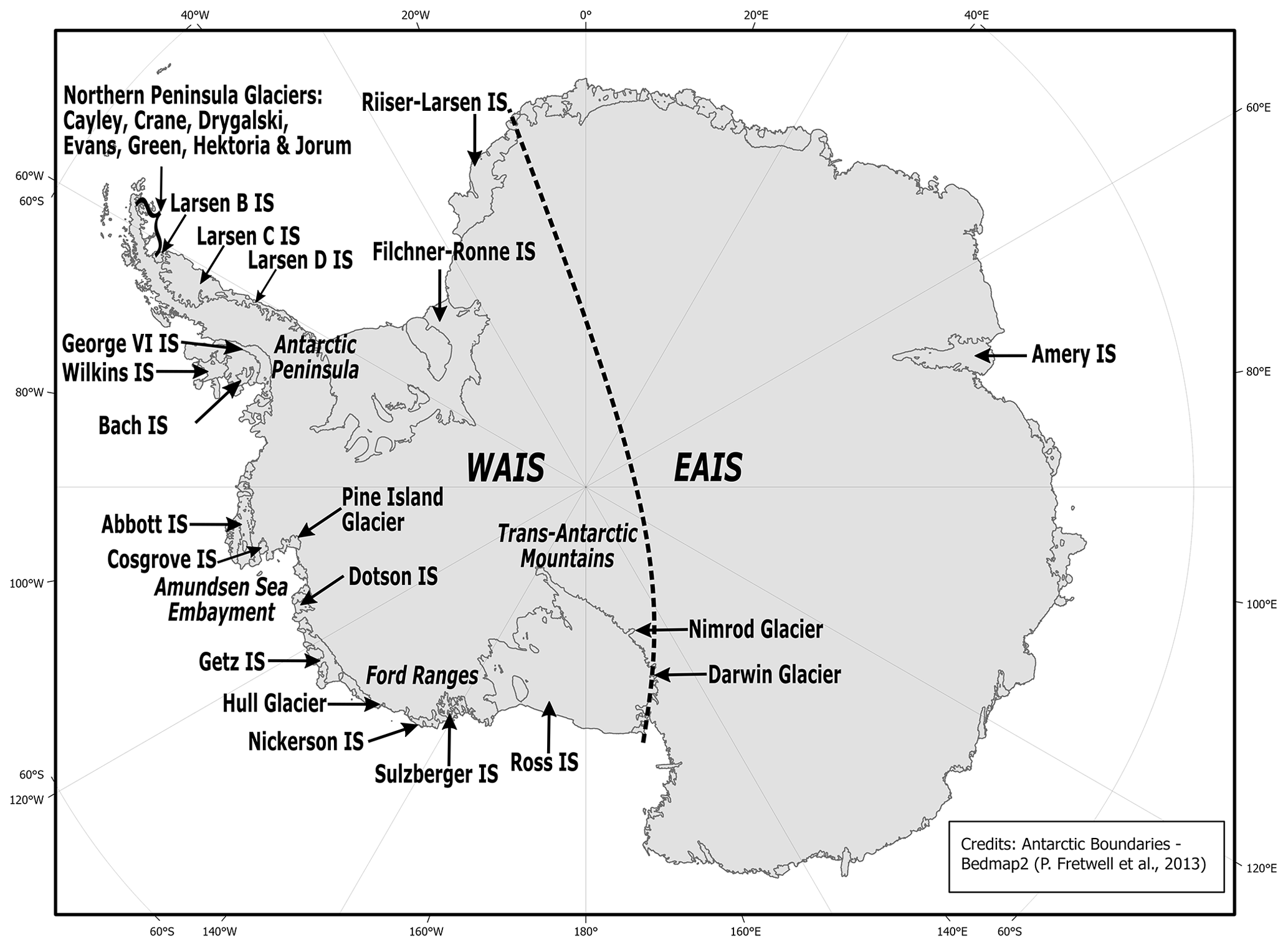
Figure 1 Map of the key locations on the Antarctic Ice Sheet referenced within the paper. Many of the labelled glaciers and ice shelves host supraglacial hydrology features in January 2017. The Antarctic boundaries are according to Bedmap2 (Fretwell et al., 2013).

Meltwater, which enters cracks, crevasses and moulins on grounded ice, drains into the sub- or englacial environments (McGrath et al., 2012; van der Veen, 2007). In Greenland, rapid delivery of surface water to the bed has been found to reduce basal friction and temporarily increase ice flow velocities by up to an order of magnitude (Tedesco et al., 2013). It has been hypothesised that mechanisms similar to those observed in Greenland may also occur in East Antarctica (Langley et al., 2016). Indeed, a recent study has shown evidence of five glaciers on the Antarctic Peninsula (Drygalski, Hektoria, Jorum, Crane and Cayley) undergoing near-synchronous speed-up events in March 2017, November 2017 and March 2018 (Tuckett et al., 2019). This suggests the surface meltwater may have entered the subglacial hydrological system.

The conditions under which drainage occurs and indeed whether lakes can cause hydrofracture, drain rapidly and affect ice shelf stability on Antarctica remain unclear. Supraglacial hydrology may exert a larger effect on Antarctica's future evolution. For example, the UN Paris Agreement's limit on the rise in global temperatures of 1.5 ^∘C (https://unfccc.int/sites/default/files/english_paris_agreement.pdf, last access: 9 December 2021) will likely cause the Antarctic Peninsula to experience irreversible, dramatic change to glacial, terrestrial and ocean systems (Siegert et al., 2019). Under this warming (1.5 ^∘C), ice shelves will experience a continued increase in meltwater production and meltwater will therefore become more extensive (Siegert et al., 2019). The impact of increased meltwater upon ice shelf stability and ice dynamics lacks understanding. Therefore mapping the distribution and evolution of the hydrological system from Earth observation has become a key priority of research.

2 Data and methods

Here, we describe the selection and pre-processing of Sentinel-2 (S2) and Landsat-8 (L8) satellite imagery, the identification of candidate water pixels (using NDWI – normalised difference water index), and the approach used to mask cloud, rock, slush, blue-ice and shaded pixels. The steps involved in post-processing the data and separating supraglacial lakes and channels are outlined. The methods differ between sensors as L8 provides thermal information (band 10), whereas S2 does not. Thresholds on individual bands (or indices) are specific to the spectral properties of each sensor and therefore require adjustment for each sensor (Moussavi et al., 2020).

2.1 Satellite imagery

In this paper, we use 1682 S2 satellite images to map supraglacial hydrology in West Antarctica. For locations where no S2 data are available, we include 604 L8 images to supplement our dataset. We assess all available scenes with cloud cover below 10 % from 1 to 31 January 2017 on the WAIS. To maximise coverage on the Antarctic Peninsula, which typically experiences more cloudy conditions, we extend the period to 10 February 2017 and use scenes with cloud cover up to 40 %.

S2 data are freely available as ortho-rectified, map-projected images containing top-of-atmosphere (TOA) reflectance data from the Copernicus Open Access Hub: https://scihub.copernicus.eu/ (last access: 3 December 2021). S2 bands 2 (blue), 3 (green), 4 (red) and 8 (near infrared – NIR) exist at a resolution of 10 m, the highest spatial resolution acquired by the sensor. In contrast, bands 1 (short-wave infrared – SWIR – Cirrus) and 11 (SWIR) are acquired at a coarse resolution of 60 and 20 m, respectively, and are therefore re-sampled to 10 m using nearest-neighbour interpolation for consistency with red, green and blue (RGB) and NIR bands (Williamson et al., 2018). The S2 pixel values represent TOA reflectance units × 10 000 and are known as TOA reflectance integers (reflectance × 10⁴).

L8 data are freely available from the United States Geological Survey (USGS) Earth Resources Observation Science (EROS) Centre (https://eros.usgs.gov, last access: 3 December 2021) and are provided as a level-1 data product comprising quantised and calibrated scaled digital numbers (DNs). Before use, we convert L8 images to TOA reflectance or brightness temperature values following the method of Chander et al. (2009). Besides conversion to TOA reflectance, the blue, green, red and NIR bands of L8 data are pan-sharpened using an intensity hue saturation method (Rahmani et al., 2010). This increases the resolution from the native 30 to 15 m for comparability with S2, which has a native resolution of 10 m. The remaining L8 bands used, 6 (SWIR, 30 m) and 10 (thermal infrared sensor, 100 m), are also re-sampled, using nearest-neighbour interpolation as with the S2 data.

2.1.1 Normalised difference water index (NDWI) thresholding

Multi-spectral satellite imagery is commonly used to detect open water on ice sheet surfaces (Moussavi et al., 2020; Williamson et al., 2018; Miles et al., 2017; Leeson et al., 2020; Stokes et al., 2019; Langley et al., 2016). These methods exploit differences in the spectral signatures of open water and snow/ice/firn at optical frequencies. The NDWI performs well in identifying supraglacial lakes in Antarctica, using either NIR and green bands (NDWI_GNIR), Eq. (1), or blue and red bands (NDWI_BR), Eq. (2) (Morriss et al., 2013; Moussavi et al., 2016; Xu, 2006; Stokes et al., 2019; Williamson et al., 2017).

$$\begin{array}{}\text{(1)}& {\displaystyle }& {\displaystyle }{\text{NDWI}}_{\text{GNIR}}={\displaystyle \frac{\text{Green Band}-\text{NIR Band}}{\text{Green Band}+\text{NIR Band}}}\text{(2)}& {\displaystyle }& {\displaystyle }{\text{NDWI}}_{\text{BR}}={\displaystyle \frac{\text{Blue Band}-\text{Red Band}}{\text{Blue Band}+\text{Red Band}}}\end{array}$$

Supervised classification algorithms are in their infancy in the supraglacial hydrology field (Dirscherl et al., 2020; Halberstadt et al., 2020), and large-scale, continental studies require validation and testing for generalisation and transferability of the methods. The aim of this study was to produce a dataset to assist such studies, and, consequently, NDWI thresholding was selected as our approach. Currently, NDWI thresholding methods are the standard approach to mapping supraglacial hydrology in Greenland and Antarctica (Morriss et al., 2013; Moussavi et al., 2016, 2020; Stokes et al., 2019; Williamson et al., 2017; Xu, 2006).

Figure 2 S2 processing chain (a). The input files are the S2 Multi-Spectral Instrument (MSI) products (RGB composite of tile T13CET_20170106 from 6 January 2017 on Pine Island Glacier b), and the output is the supraglacial lake and channel binary (surface water – not water) classification (c). Imagery was accessed from European Space Agency's (ESA) Copernicus Scihub, http://scihub.copernicus.eu (last access: 3 December 2021).

Open water features appear as a dark blue colour in optical satellite images because of the rapid attenuation of red light in water relative to blue light. NDWI ratios are, therefore, well suited to map lakes as they exploit the properties of lakes which make them more easily distinguished from ice at short optical wavelengths (blue wavelengths) and from the snow at long optical wavelengths (red wavelengths) (Morriss et al., 2013; Liang et al., 2012; Pope et al., 2016; Yang and Smith, 2013; Sneed and Hamilton, 2007; Box and Ski, 2007; Moussavi et al., 2020). However, identifying supraglacial lake and channel pixels using NDWI alone is insufficient because slush, rocks, clouds and shadows can be spectrally similar to water (Moussavi et al., 2020). For this reason, they require additional processing steps to identify and mask these features in each image. Additional, manual post-processing steps described in Sect. 2.1.3 “Post-processing”, carried out by human experts, provide data which are of much higher quality than spectral thresholding alone. The processing chain used to map supraglacial lakes and channels in S2 and L8 imagery is shown in Figs. 2 and 3.

2.1.2 Cloud, rock masking and elimination of slush, blue-ice and shaded pixels

Thresholds are applied to individual bands, spectral indices and band combinations such that we isolated water pixels based on multiple spectral properties. The first step in this process is to remove areas of exposed rock which are often misclassified as water by the NDWI algorithm (Figs. 2 and 3). We generate rock masks for S2 images by defining a threshold (<0.9) on a normalised difference snow index (NDSI; Eq. 3). The NDSI divides the difference in the green and SWIR bands by the sum of the bands. To remove snow and cloud from the rock mask, thresholds are applied to blue (<4000 reflectance × 10⁴) and green (<4000 reflectance × 10⁴) bands (Moussavi et al., 2020). Alongside rock, this mask is also used to remove areas of open ocean which are found next to ice shelves.

$$\begin{array}{}\text{(3)}& {\displaystyle }{\displaystyle }\text{NDSI}={\displaystyle \frac{\text{Green Band}-\text{SWIR Band}}{\text{Green Band}+\text{SWIR Band}}}\end{array}$$

We performed rock and seawater masking for L8 images by applying a threshold (>650) to the ratio of the blue band and thermal infrared band (TIRS; Eq. 4). To remove snow from the rock mask, a threshold is applied to the blue band (<0.35 reflectance) (Moussavi et al., 2020).

$$\begin{array}{}\text{(4)}& {\displaystyle }{\displaystyle \frac{{\text{TIRS}}_{\mathrm{1}}\text{ Brightness Temperature}}{\text{Blue Band}}}\end{array}$$

We generated cloud masks for S2 imagery by applying thresholds on the blue band of >6000 reflectance × 10⁴ and <9700 reflectance × 10⁴ and thresholds of >1100 reflectance × 10⁴ and >30 reflectance × 10⁴ to SWIR and SWIR Cirrus, respectively (Moussavi et al., 2020) (Fig. 2). We employ the cloud mask for L8 imagery using thresholds on the blue (>0.60 reflectance and <0.95 reflectance) and SWIR bands (>0.10 reflectance) and a threshold of <0.80 on the NDSI equation (Moussavi et al., 2020). For bands that have been resampled to increase spatial resolution (SWIR and SWIR Cirrus for S2, SWIR and long-wave infrared – LWIR – for L8), unwanted edge effects are introduced around the edge of the tiles during the up-sampling process. Thresholds on the red band (>0 reflectance for L8) and blue band (>0 reflectance × 10⁴ for S2) are therefore used to remove those edge effects.

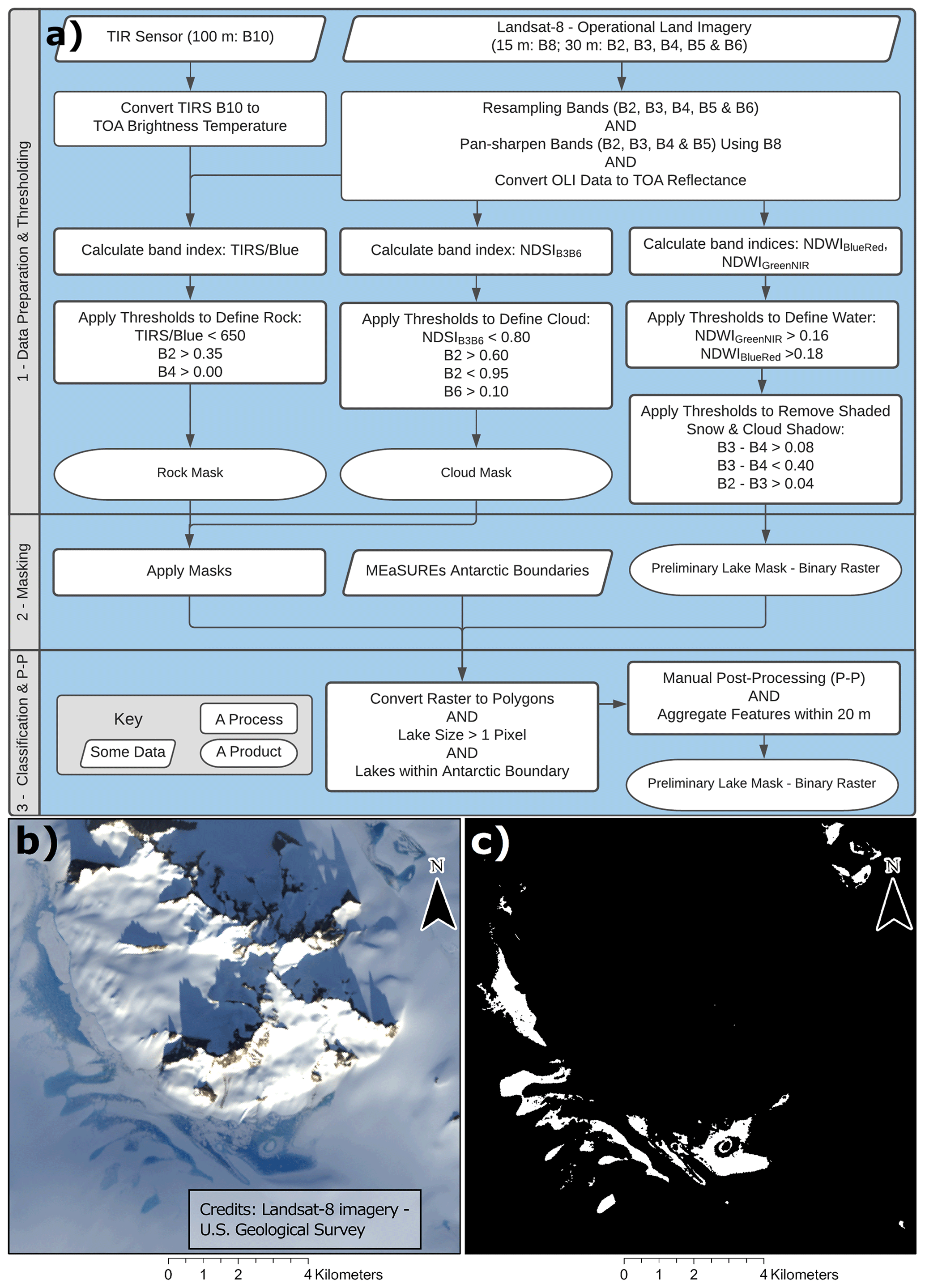
Figure 3 L8 processing chain (a). The input files are the L8 Operational Land Imager (OLI) and Thermal Infrared Sensor (TIRS) products (RGB composite of tile LC08_L1GT_192129_20170118 from 18 January 2017 on Pine Island Glacier b), and the output is the final supraglacial lake and channel dataset (c) in raster and vector format. Imagery was accessed from US Geological Survey, http://earthexplorer.usgs.gov (last access: 3 December 2021).

We extracted water pixels using thresholds on two NDWI calculations, Eqs. (1) and (2). The first step to calculate NDWI_GNIR (Eq. 1) sets a threshold of 0.16 (for both sensors), above which pixels are considered to have the potential to be water. As stated above, with this threshold alone, the output typically contains slush, blue-ice, shaded rock and cloud shadow pixels. Rock and cloud pixels are removed in their respective masking processes. To reduce misclassification of slush and blue-ice pixels, a threshold of 0.18 is further applied to NDWI_BR (Moussavi et al., 2020). To highlight the difference between light attenuation properties in water and shaded snow surfaces, thresholds are applied to a combination of blue, green and red bands (Moussavi et al., 2020). We filtered shaded snow and cloud shadows using $\mathrm{800}\left(\mathrm{0.08}\right)<\text{green}-\text{red}<\mathrm{4000}\left(\mathrm{0.40}\right)$ and $\text{blue}-\text{green}>\mathrm{400}\left(\mathrm{0.04}\right)$ for S2 reflectance × 10⁴ (and L8 reflectance). Previous analyses on the distribution of pixel values from Landsat-8 and Sentinel-2 tiles (Figs. 2 and 4 in Moussavi et al., 2020) represent the different spectral properties of lakes, slush, snow, shaded snow, clouds, cloud shadows, sunlit rocks and shaded rocks. This analysis was used to determine the thresholds in their approach. The thresholds we select for rock and cloud masking were adapted from their approach (Moussavi et al., 2020) and the source code from GitHub (Moussavi, 2019). Thresholds were selected to produce maximum lake delineation, with any additional false positives created removed in the manual post-processing stage. The analysis conducted to select the thresholds, the NDWI thresholding approach and the additional band filters is described in Appendix A.

2.1.3 Post-processing

The processing chain outlined generates a binary raster of “water” and “not water” pixels. We subsequently converted groups of water pixels in the raster into polygons representing discrete lakes or channels. Features smaller than two pixels (200 m² in S2 and 450 m² in pan-sharpened L8 imagery) are removed from the datasets as such features are considered to be below the detection limit of the sensors and more likely to be areas of slush rather than open water (Pope et al., 2016). In addition, all features that are beyond the boundary of Antarctica (i.e. not on grounded ice or floating ice shelves) based on the MEaSUREs coastline of Antarctica (Mouginot et al., 2017) are removed accordingly.

Despite the rock, cloud, and shadow masking steps that are applied during image processing, areas of shadow, cloud, rock, crevassing and blue ice can still be misclassified as water and thus erroneously converted into lake and channel polygons. We manually removed these “false positives”, regarding their appearance in true colour (RGB) composite images during post-processing. Approximately 50 % of images required such post-processing step mainly because of the presence of misclassified rock and/or shadow. Up to ∼39 % (6708) of all 17 186 polygons (∼42 % of area) delineated automatically are false positives upon manual inspection and were subsequently deleted. We identify 10 478 supraglacial features in this study. Most of all, false positives are linked to shaded rock, with either rock in shadow or snow cast into shadow by rock. A few densely populated crevassed regions contribute to ∼20 % of misclassified features, but because of their small size (<10 pixels), this represents a much smaller percentage of the total misclassified area.

Although no dedicated checks are carried out to assess the number of false negatives, during the visual inspection for false positives, no large features (>50 pixels) were found to be excluded. Minor features (<5 pixels) may remain uncharted. However, their influence on the overall area mapped – and therefore the volume of surface water – is likely to be minimal. Finally, overlapping polygons from each sensor, location and time instance throughout January 2017 are dissolved, and polygons within a distance of 20 m are aggregated to provide a more continuous delineation of hydrological connectivity.

2.2 Accuracy assessment

We tested the fidelity of our method by comparing our results with 97, 184 and 105 (119, 135 and 46) manually delineated lakes and channels from S2 (and L8) imagery on test sites crossing the grounding line on Amery, George VI and Bach ice shelves, respectively (Fig. 1). These ice shelves vary in their glaciological and climatological characteristics, which result in a range of feature geometries and settings that are considered to represent the whole of Antarctica. In each of the three regions, we selected test regions that encompass extensive surface hydrological meltwater and host close to 100 individual supraglacial features of varying sizes. This resulted in test regions measuring 210 km² (for Amery Ice Shelf – IS) and 100 km² (for George VI – GVI – IS and Bach IS).

Amery IS, the third largest ice shelf in Antarctica, is in East Antarctica. The chosen test site on Amery IS is well suited for automated processing due to clear spectral differences between surface water and ice pixels in the region. However, a small area of blue ice, which has a similar spectral signature to that of open water, is challenging to differentiate automatically. George VI (GVI), one of the largest ice shelves on AP, constrained between the western side of the AP and Alexander Island, loses most of its mass to melt rather than calving (Roberts et al., 2008). GVI IS has two ice fronts, one situated around 500 km further north, and so experiences different climatic conditions (Cook and Vaughan, 2010). The test site, situated around the middle of the ice shelf, crosses the grounding line of Alexander Island and contains rock and shaded pixels, presenting a more difficult task for the method. Bach Ice Shelf is on the coast of Alexander Island, to the east of the AP. Although to date it has shown relative stability in an area where other ice shelves (particularly Wilkins IS) have undergone major collapse (Humbert and Braun, 2008; Scambos et al., 2009), Bach Ice Shelf could be the next ice shelf under threat of break-up (Cook and Vaughan, 2010). The test region on the Bach Ice Shelf offers a contrasting stress regime (unconfined vs. confined flow) to that of the GVI ice shelf, which has the potential to create different lake geometry (Scambos et al., 2000; Cook and Vaughan, 2010).

We manually delineated lakes and channels in each test area using true colour (RGB) composites of S2 and L8 data. Three separate “expert” users delineated each area (with expertise in remote sensing of supraglacial hydrology). We combined the three manual inventories to form a high-fidelity reference dataset of the lake and channel features in which only pixels that are unanimously assigned as “water” (i.e. identified as water by all three users) are included. To assess the performance of our method, we calculated confusion matrices that compared manual (Man.) and the final automated (Auto.) datasets (following post-processing) on a per-pixel basis. From the confusion matrices, sensitivity, specificity and accuracy have been derived (Eqs. 5, 6 and 7).

The sensitivity, or true positive rate, is the number of true positive (or Man. Water : Auto. Water in a confusion matrix) predictions divided by the number of manually identified water pixels in the test data. It is a measure of how well we correctly identified surface water pixels.

$$\begin{array}{}\text{(5)}& {\displaystyle }{\displaystyle }\text{Sensitivity}={\displaystyle \frac{\text{Man. Water}:\text{Auto. Water}}{\text{Total Man. Water}}}\end{array}$$

The specificity, or true negative rate, is the number of true negative predictions (or Man. Not Water : Auto. Not Water) divided by the number of manually identified non-water pixels in the test data. It is a measure of how well all other non-water pixels are identified.

$$\begin{array}{}\text{(6)}& {\displaystyle }{\displaystyle }\text{Specificity}={\displaystyle \frac{\text{Man. Not Water}:\text{Auto. Not Water}}{\text{Total Man. Not Water}}}\end{array}$$

We calculated the accuracy by dividing the sum of true positive and true negative predictions by the total number of pixels. It gives a quantitative assessment for the accuracy of all pixels, both water and non-water.

$$\begin{array}{ll}{\displaystyle }& {\displaystyle }\text{Accuracy}\\ \text{(7)}& {\displaystyle }& {\displaystyle }={\displaystyle \frac{\begin{array}{c}\text{Man.}\\ \text{Manual}\end{array}:\begin{array}{c}\text{Auto.}\\ \text{Manual}\end{array}+\begin{array}{c}\text{Man. Not}\\ \text{Water}\end{array}:\begin{array}{c}\text{Auto. Man}\\ \text{Water}\end{array}}{\text{All Pixels}}}\end{array}$$

We computed sensitivity, specificity and accuracy values for each test site and sensor (Table 1). Across both sensors, sensitivity ranges between 61.4 % and 96.4 %, specificity between 97.9 % and 99.9 %, and accuracy between 97.1 % and 99.3 %. On average, S2 yields a higher sensitivity (85.3 % vs. 77.6 %) than L8, while values for specificity and accuracy have higher averaged values for L8 than S2.

Table 1 Sensitivity (sen.), specificity (spec.) and accuracy (acc.) of the S2 and L8 methods for each of the test sites: Amery, George VI and Bach ice shelves and the mean values across sensors and sites for each.

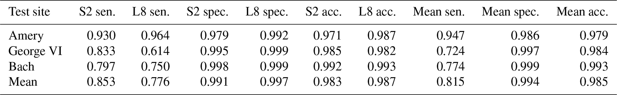
The large range in sensitivity is likely because of shallow lakes (deemed so by manual users) being classified as ice by the NDWI threshold, especially on GVI and Bach ice shelves, where there are many shallow lakes. In contrast, the range in specificity (i.e. how well non-water pixels are identified) is smaller because the analysis was carried out after manual post-processing, and misclassified pixels were already removed. This suggests that, for applications for which identifying shallow lakes is important, we may further improve the sensitivity by incorporating additional manual checks for false negatives into the NDWI thresholding approach.

3 Results and discussion

3.1 Distribution of supraglacial lakes and streams in West Antarctica

We used 1682 S2 and 604 L8 scenes to map 10 478 individual supraglacial features in West Antarctica, including the Antarctic Peninsula (Fig. 4). The dataset comprises 10 223 SGLs and 255 channels.

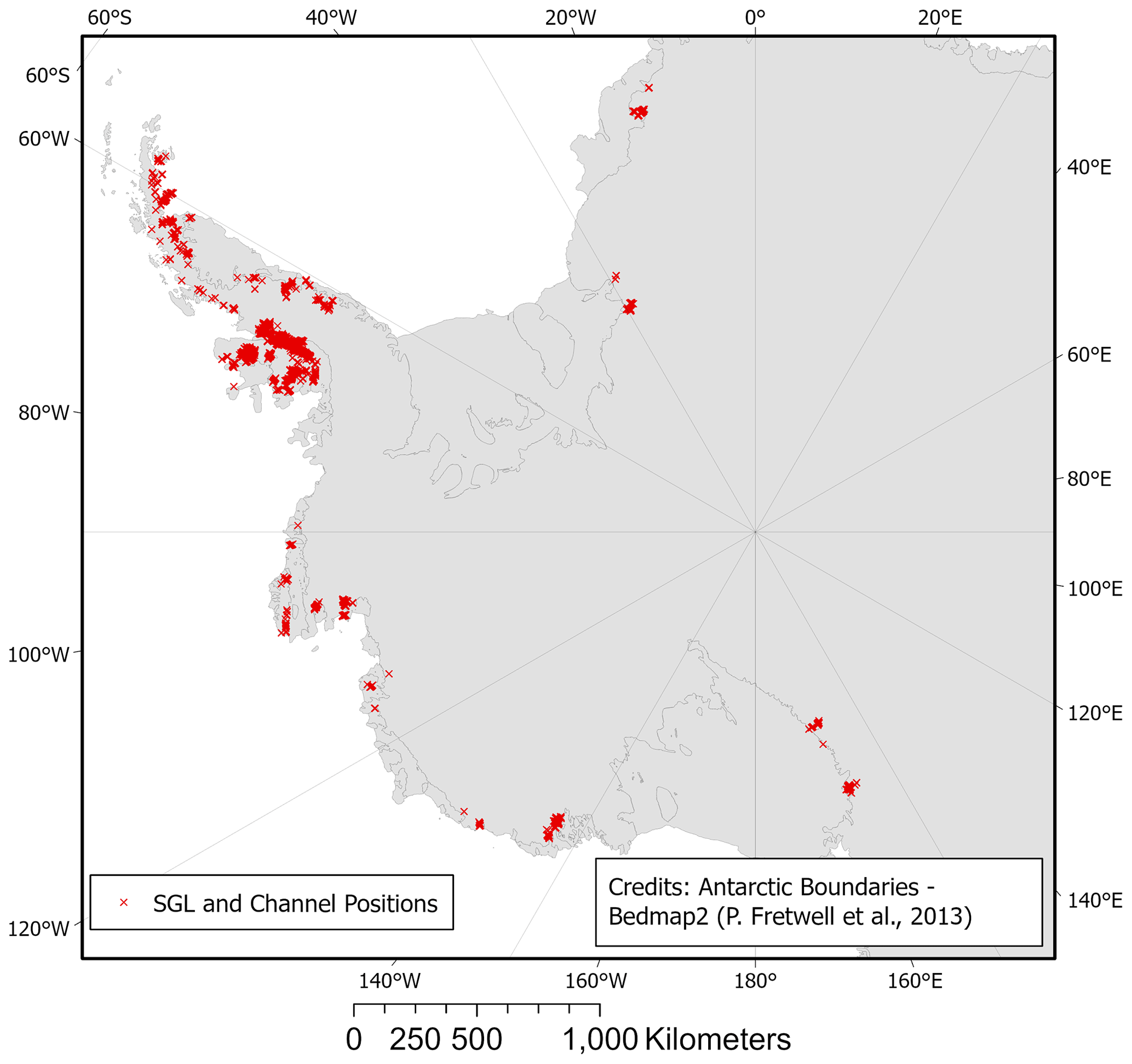
Figure 4 Location of the 10 478 SGLs and channels on the WAIS and AP represented by the red crosses as mapped in S2 and L8 imagery from January and February 2017. Antarctic boundaries are according to Bedmap2 (Fretwell et al., 2013).

We found SGLs in expected regions on and around the grounding zone of the Antarctic Peninsula ice shelves including Larsen C (∼130 lakes), Larsen D (∼250), George VI (∼5550), Wilkins (∼1450) and Bach (∼950). We also discovered lakes on grounded ice close to where the remnants of Larsen A (∼10) and B (∼150) ice shelves are located. Sulzberger ice shelf (∼290), Pine Island Glacier (∼360), Riiser-Larsen (∼240), and around the Trans-Antarctic Mountains and Ross Ice Shelf on Darwin (∼270) and Nimrod (∼90) glaciers are identified to host SGL activity in this study and others (Kingslake et al., 2017). Studies identifying lakes in the Ford Ranges region – on Hull Glacier (∼45) and Nickerson ice shelf (∼80) – and in Amundsen Sea region – on Dotson (∼35), Abbot (∼125) and Cosgrove (∼45) ice shelves – were published for the first time recently (Dirscherl et al., 2020; Arthur et al., 2020), and we confirm the occurrence of lakes here during January 2017. We identified 255 supraglacial channels on or around the margin of Larsen C, Larsen D, remnants of Larsen B, GVI, Bach, Wilkins, Riiser-Larsen, Dotson and Sulzberger ice shelves and near to the Hull and Pine Island glaciers. We identified supraglacial meltwater for the first time on the Getz Ice Shelf, with one lake crossing the grounding line, while a further four border the ice shelf (Fig. 5). It has been suggested that increased surface melt on the Getz Ice Shelf will lead to collapse unless active surface drainage can mitigate the effect of surface loading by exporting water to the ocean (Bell et al., 2018).

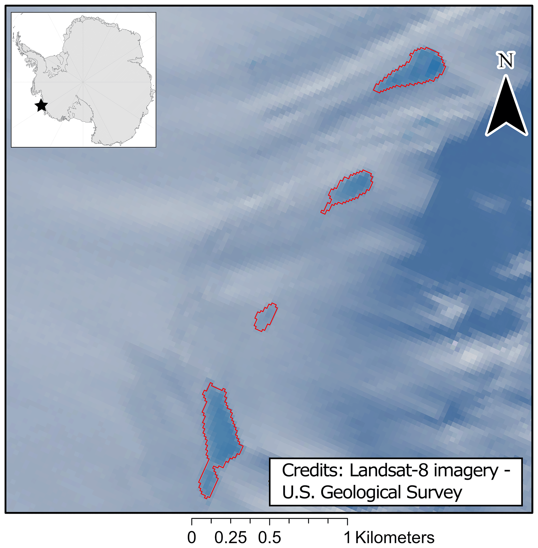
Figure 5 Lakes identified for the first time in the western Amundsen Sea sector of West Antarctica, with the largest, southernmost lake of the four crossing the grounding line of the Getz Ice Shelf. The image is a true colour composite of L8 satellite imagery, tile LC08_L1GT_166131_20170112 from 12 January 2017. The red outlines are the lake polygons resulting from our NDWI threshold approach. Inset: Getz IS and lake locations in Antarctica. Imagery was accessed from US Geological Survey, http://earthexplorer.usgs.gov (last access: 3 December 2021).

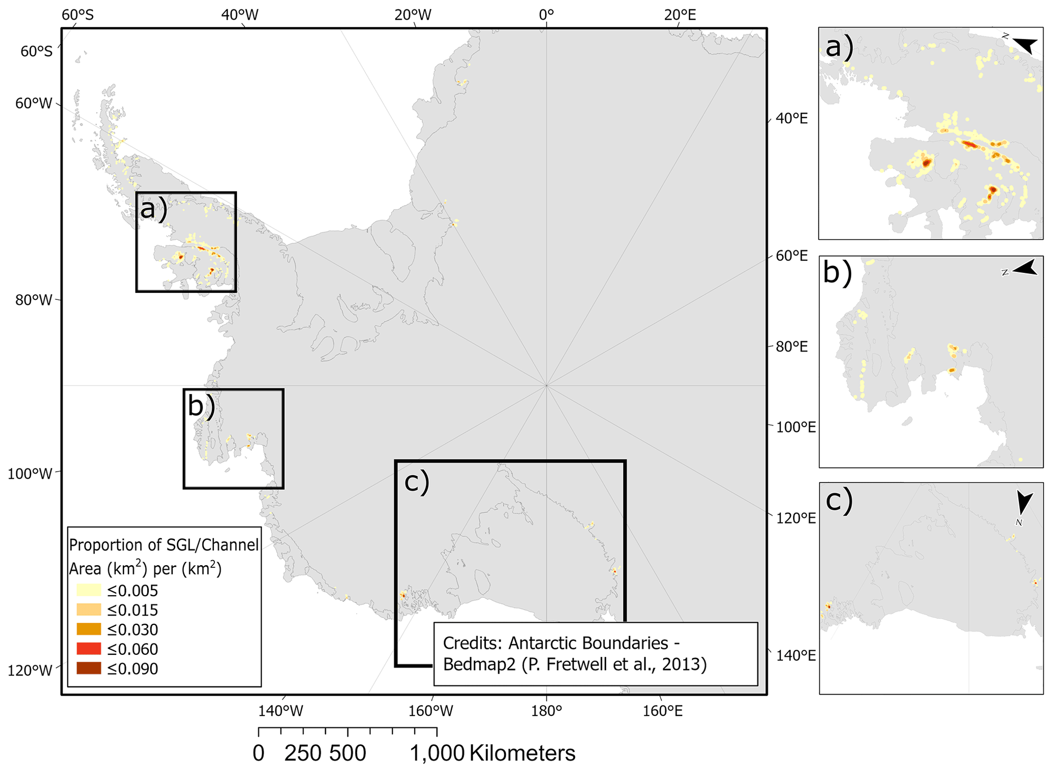
Figure 6 The proportion of lake and channel area covered by meltwater per square kilometre in each region on WAIS and AP where surface water is identified. Inset: high cover regions on (a) AP (George VI, Wilkins and Bach ice shelves), (b) Amundsen Sea region (Pine Island Glacier), and (c) Ford Ranges (Sulzberger IS) and Trans-Antarctic Mountains (Ross IS, Darwin and Nimrod glaciers). Antarctic boundaries according to Bedmap2 (Fretwell et al., 2013).

The proportion of area covered by meltwater in a localised region (Fig. 6) was calculated using the cumulative lake and channel area in a hexagonal bin. Each bin measured 100 m between parallel sides of the hexagon, while any feature within a search radius of 5 km (longest feature: ∼4.7 km) contributed to the proportion of the bin in question. The proportions range from 0 (where no lakes are within 5 km of a bin) to 0.089 km² of meltwater area per 1 km², with the highest density regions on the Antarctic Peninsula (George VI, Wilkins and Bach ice shelves), Ford Ranges, Trans-Antarctic Mountains and Pine Island Glacier. George VI, which measures ∼24 000 km² (Cook and Vaughan, 2010), has total meltwater area of 29.4 km² and a percentage cover of supraglacial meltwater across the ice shelf of 0.12 %. Wilkins (meltwater area: 14.0 km²; total area: ∼11 000 km²; Cook and Vaughan, 2010) and Bach (meltwater area: 13.0 km²; total area: 4500 km²; Cook and Vaughan, 2010) ice shelves have maximum percentage cover of 0.13 % and 0.29 %, respectively. Areas with a low proportion of area covered, hosting just a few lakes, include Getz IS, the western margin of the Filchner-Ronne IS, Hull Glacier and on James Ross Island off the coast of the northern AP.

We have assessed area distribution for SGLs and channels (Fig. 7). The total area covered by lakes (114.7 km²) and channels (4.7 km²) was found to be 119.4 km². The proportions of features on grounded ice (GI), floating ice shelf (IS) and crossing the grounding line (GL) are computed (Fig. 8). Distributions of glaciologically important parameters (Fig. 9b–f and h) for the 10 478 supraglacial features, including distance to the grounding line, exposed bedrock and coastline, were calculated. Ice surface elevation, slope and velocity were observed for each feature, and their distribution was plotted. Finally, the distribution of meltwater volume was calculated (Fig. 9a).

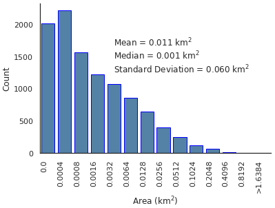
Figure 7 Distribution of SGL and channel area (km²) on WAIS and AP. Note: bin sizes double from left to right. Values for mean, median and standard deviation for the distribution are included in the figure.

Figure 8 Area split between channels and lakes completely on grounded ice (GI), crossing the grounding line (GL) and completely on floating ice shelves (IS) across the WAIS and AP.

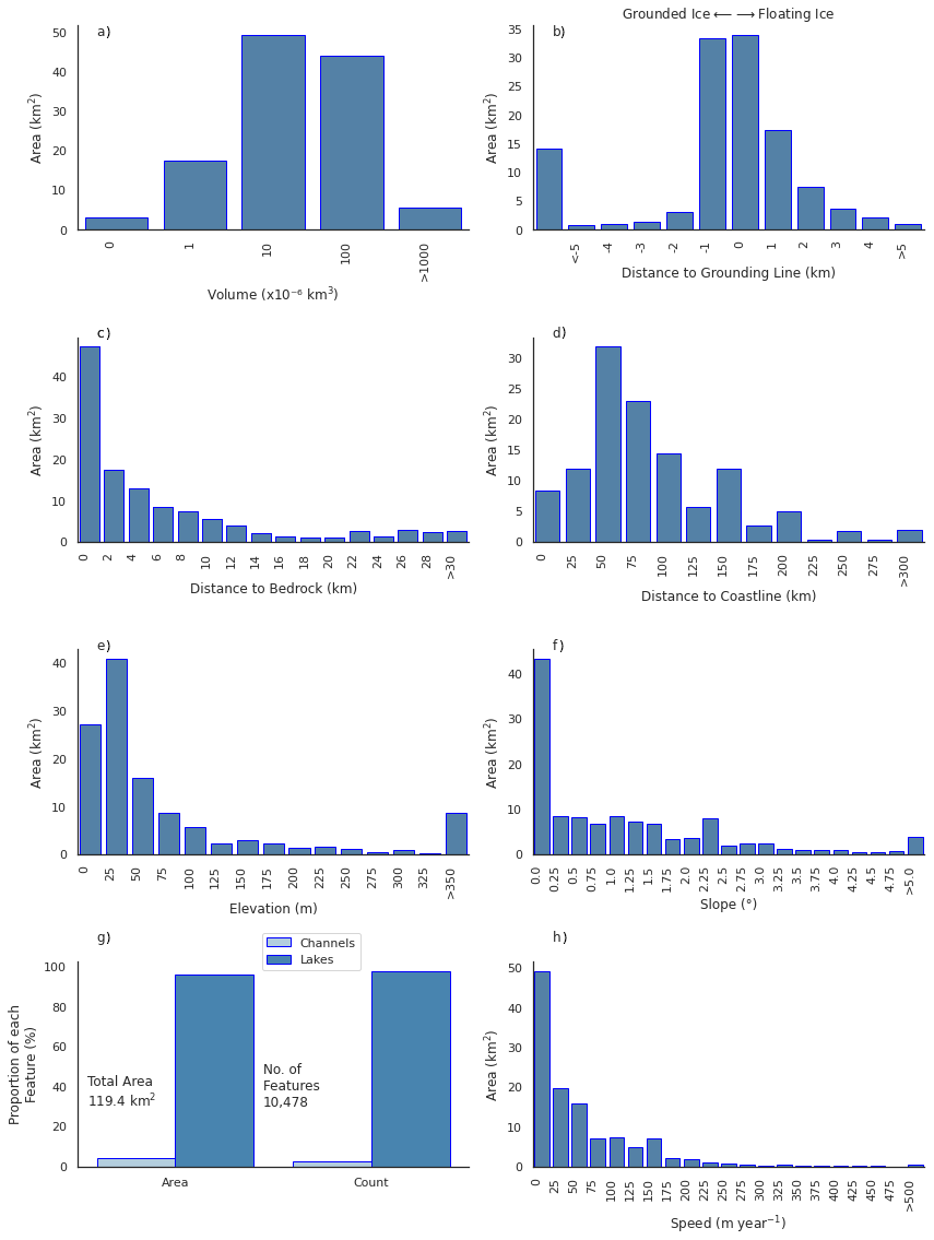
Figure 9 Area distributions of supraglacial lakes and channels on the WAIS and AP according to various glaciological variables. (a) Individual feature volumes from the area–volume scaling relationship (Eq. 8); (b) distance of each feature to the grounding line (negative values indicate lake and channel positions further inland from the grounding line); (c) distance of each feature to nearest exposed bedrock; (d) distance of each feature to the ice margin or coastline; (e) elevation at the centroid of each feature; (f) the surface slope at the centroid of each feature; (g) area and frequency split between channels and lakes on the WAIS and AP; (h) ice flow speed for each feature. Imagery was accessed from European Space Agency's (ESA) Copernicus Scihub, http://scihub.copernicus.eu (last access: 3 December 2021), and US Geological Survey, http://earthexplorer.usgs.gov (last access: 3 December 2021).

The largest lake identified (∼2.9 km²) intersects the grounding line of the Sulzberger ice shelf, although most lakes and channels are an order of magnitude smaller. For example, we found 8700 (83 %) of the features to have an area of less than 0.1 km² (Fig. 7). Lakes make up 96.1 % of total feature area and 97.6 % of all features (Fig. 9g). More than half (54.9 %) of the total open water area was entirely on floating ice, with 27.3 % on grounded ice entirely (Fig. 8). Among the features on grounded ice, the lake found farthest inland of the grounding line is on the Antarctic Peninsula, 47.2 km from the George VI IS. In terms of floating ice, the lake found farthest from the grounding line is also on George VI at a distance of 12.6 km. Over half of the open water area (56.4 %) is within 1 km of the grounding line according to Bedmap2 (Fretwell et al., 2013), with 17.8 % of total open water area intersecting the grounding line (Fig. 9b).

Exposed bedrock has a lower albedo than snow or ice, which can increase the absorption of incoming solar energy, leading to higher rates of melting within the local area. We find that 78.1 % of the total feature area (and 80.1 % of all features) exists within 10 km of exposed bedrock (Fig. 9c). Lakes are also found at substantial distances inland (Fig. 9d), including over 504 km away from the closest coastline. Most of the open water, however (64.9 % of features and 63.1 % of area), was found within 100 km of the coast, according to MEaSUREs data for the coastline of Antarctica (Mouginot et al., 2017; Rignot et al., 2013).

We found most features (80.8 %, representing 77.5 % of the total feature area) at low elevations (Fig. 9e), i.e. between 0 and 100 $\mathrm{m}\mathrm{a}.\mathrm{s}.\mathrm{l}.$, while 87 lakes and channels (or 0.4 % of area) were at elevations greater than 1000 $\mathrm{m}\mathrm{a}.\mathrm{s}.\mathrm{l}.$, with two (in the mountain region around 40 km east of GVI ice shelf) as high as 1306 $\mathrm{m}\mathrm{a}.\mathrm{s}.\mathrm{l}$. Most lakes and channels (57.9 %) occur on surface slopes <1^∘ (Fig. 9f). This accounts for 55.7 % of the total area.

To estimate the ice flow velocity at the geometric centroid of each feature, we extracted the ice surface velocity from the MEaSUREs InSAR-Based Antarctica Ice Velocity Map (Rignot et al., 2017; Rignot et al., 2011; Mouginot et al., 2012). Ice flow velocities in lake-covered regions ranged from ∼0 to >1357 m yr⁻¹; however 57.8 % of the total feature area (and around 47 % of the total features) was on ice flowing slower than 50 m yr⁻¹ (Fig. 9h).

To estimate the volume of water contained within each feature, we use an area–volume (A−V, Eq. 8) scaling relationship from the literature (Stokes et al., 2019). Based on this relationship, the total volume of meltwater stored in supraglacial lakes and streams is estimated to be 0.085 km³ across the entire WAIS and AP.

$$\begin{array}{}\text{(8)}& {\displaystyle }{\displaystyle }V=\mathrm{7.16}\times {\mathrm{10}}^{-\mathrm{4}}A\end{array}$$

Due to proportionality between area and volume, the feature containing the maximum volume of water (∼0.002 km³) is the lake on the Sulzberger ice shelf, identified as the largest by surface area. A total of 86.9 % (>9000 features) of all lakes and channels have volumes between 0 and 0.0001 km³, while this range accounts for only 17.2 % of total area. Conversely, 41.4 % of the total lake and channel area is represented by just 144 features that have a volume greater than 0.0001 km³.

3.2 Lake vs. channel features

The increased spatial resolution offered by the current generation of optical satellite sensors, such as S2, makes mapping supraglacial rivers and channels possible. Here, in contrast to previous studies in Antarctica, we distinguish between lakes and channels using a K-means clustering approach (Arthur and Vassilvitskii, 2007), combining six shape index metrics. The first, a standard area : perimeter ratio (A:P) (Eq. 9), divides the total area of a feature (A) by the length of its perimeter (P).

$$\begin{array}{}\text{(9)}& {\displaystyle }{\displaystyle }A:P={\displaystyle \frac{A}{P}}\end{array}$$

Second, we use the iso-perimetric quotient (IPQ) (Li et al., 2013), i.e. the ratio of the area of the feature to the area of a circle whose circumference, C, is equal to the perimeter. It is also known as the Polsby–Popper score when it is used to quantify the degree of gerrymandering of political districts (Polsby and Popper, 1991).

$$\begin{array}{}\text{(10)}& {\displaystyle }{\displaystyle }\text{IPQ}={\displaystyle \frac{A}{\mathit{\pi }{\left(\frac{C_P}{\mathrm{2}\mathit{\pi }}\right)}^{\mathrm{2}}}}={\displaystyle \frac{\mathrm{4}\mathit{\pi }A}{P^{\mathrm{2}}}}\end{array}$$

Providing spatial analysis of complex geographical features can be characterised by the fractal dimension. The fractal dimension index (Fractal) (Chen, 2020) reflects shape complexity across a range of spatial scales. Therefore, it overcomes one of the major limitations of the straight perimeter : area ratio as a measure of shape complexity. Depending on the number of vertices in a polygon, the fractal dimension index can be a variety of logarithmic ratios (Chen, 2020) (Eq. 11).

$$\begin{array}{}\text{(11)}& {\displaystyle }{\displaystyle }\text{Fractal}={\displaystyle \frac{\mathrm{2}\log \left(\frac{P}{\mathrm{4}}\right)}{\log \left(A\right)}}\end{array}$$

Another metric is the ratio of the feature area to the area of a minimum bounding circle (A_MBC) which is needed to enclose the feature (Eq. 12). This ratio is known as the Reock score (Reock, 1961).

$$\begin{array}{}\text{(12)}& {\displaystyle }{\displaystyle }\text{Reock}={\displaystyle \frac{A}{A_{\text{MBC}}}}\end{array}$$

To measure compactness of the feature (i.e. how neatly the area fits within the perimeter – the most compact shape is a circle) the Schwartzberg score (Azavea Incorporated, 2010) can be calculated (Eq. 13). It is the ratio of the perimeter of the feature to the circumference of a circle, C_A, whose area is equal to the area of the feature.

$$\begin{array}{}\text{(13)}& {\displaystyle }{\displaystyle }\text{Schwartzberg}={\displaystyle \frac{\mathrm{1}}{\frac{P}{C_A}}}={\displaystyle \frac{C_A}{P}}={\displaystyle \frac{\mathrm{2}\mathit{\pi }\sqrt{\frac{A}{\mathit{\pi }}}}{P}}\end{array}$$

The final metric, a width : length ratio (W:L) (Eq. 14) is calculated as the ratio of the width (W_MBR) to the length (L_MBR) of the minimum bounding rectangle, which surrounds the feature. The minimum bounding rectangle is the smallest (by width) required to enclose the full area of the feature.

$$\begin{array}{}\text{(14)}& {\displaystyle }{\displaystyle }W:L={\displaystyle \frac{W_{\text{MBR}}}{L_{\text{MBR}}}}\end{array}$$

The shape indices (Eqs. 9–14) were computed for every polygon in the final dataset (Table 2). Unsupervised K-means clustering (Arthur and Vassilvitskii, 2007) was carried out in 6-dimensional space using each of the six shape indices through the “multivariate clustering” tool in ArcGIS Pro Version 2.5.2 (https://pro.arcgis.com/en/pro-app/latest/tool-reference/spatial-statistics/multivariate-clustering.htm, last access: 9 December 2021). K-means algorithms identify a starting point (seed) from among the supraglacial features to grow each cluster. We randomly selected the first seed, while we chose subsequent seeds by directing the selection to seeds farthest in data space from the existing seeds. Small lakes, below 500 m² in area, introduced noise to the classification and were labelled as lakes before clustering.

Table 2 Value of each individual shape index (Eqs. 9–14) for the feature type defined in Fig. 10.

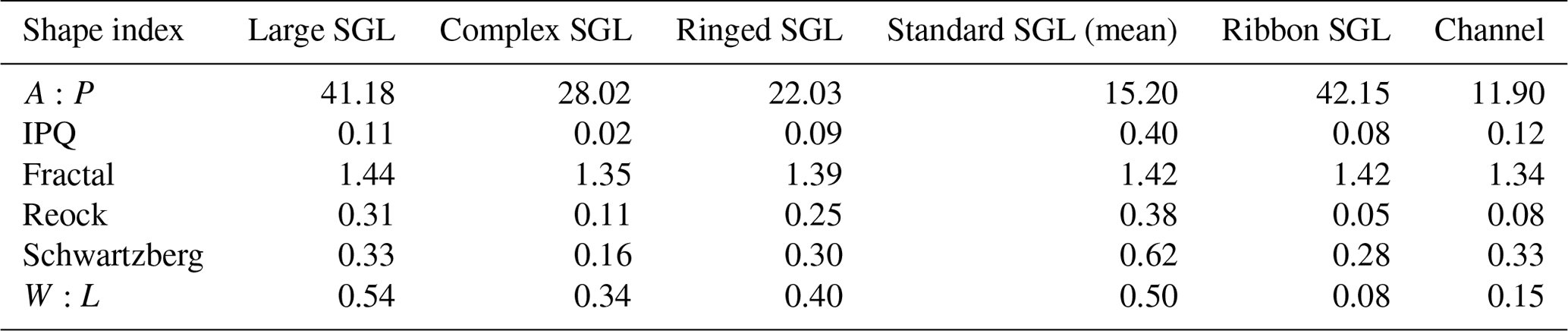
The K-means approach results in 20 distinct clusters. These clusters were manually determined to be lakes or channels of varying shapes and sizes (Fig. 10). Samples from 6 of the 20 clusters are shown in Fig. 10, with the corresponding value for each shape index in Table 2. As expected, ribbon lakes are similar to channels in most metrics as both take long, narrow forms. However, the A:P (Eq. 9) value differs vastly between channels and ribbon SGLs. The values displayed for A:P, Fractal, Reock and W:L (Eqs. 9, 11, 12 and 14) demonstrate clear differences between channels and all other lake classes, while IPQ and Schwartzberg (Eqs. 10 and 13) are useful in delineating standard, smaller lakes from channels. Through this method, we identify 10 223 lakes and 255 channels to be present during January 2017 on the WAIS and AP (Fig. 10).

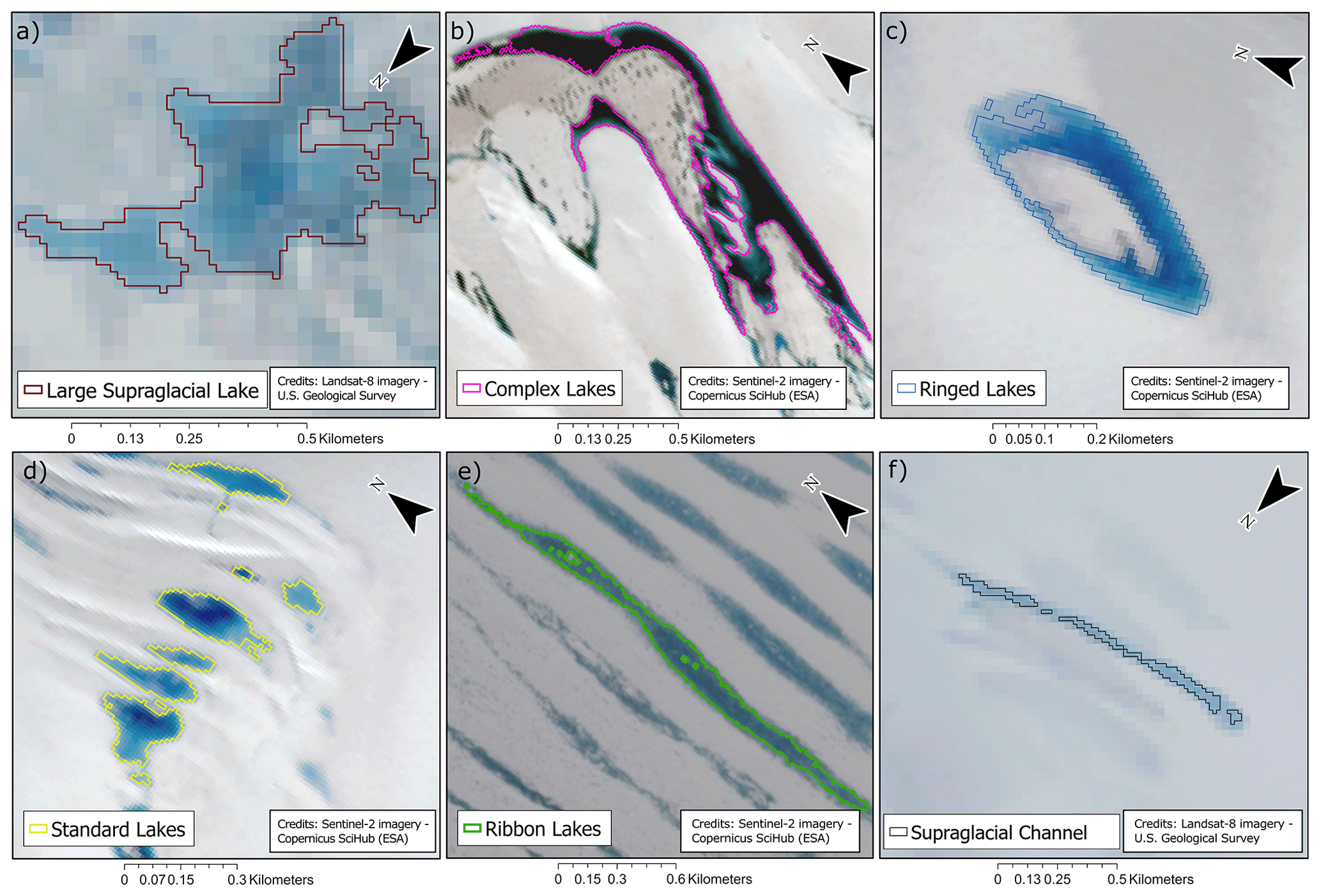
Figure 10 Outlines of supraglacial features over RGB composites from S2 and L8 imagery. These outlines demonstrate six of the distinct clusters from the K-means approach. (a) A large SGL covering 0.20 km² on Hull Glacier (Fig. 1); (b) complex SGL with area of 0.35 km² on Bach IS (Fig. 1); (c) ring lake with area of 0.05 km² on Bach IS; (d) 11 “standard” SGLs on Bach IS with areas ranging from 300 m² to 0.02 km²; (e) ribbon lake on GVI IS (Fig. 1) which spans 2.6 km and covers 0.19 km²; and (f) discontinuous supraglacial channel spanning 1.3 km and covering 0.04 km² near Hull Glacier. RGB composites formed from L8 tile LC08_L1GT_022114_20170111 (a, f) from 11 January 2017 and S2 tiles T18DXF_20170129 (b, c, d) from 29 January 2017 and T19DEB_20170103 (e) from 3 January 2017.

The values reported for accuracy, sensitivity and specificity (Table 1, Sect. 2.2) are for the thresholding approach, which consists of all water pixels, including channels and lakes. Although it would be valuable to provide validation metrics for the classification of water into channels and lakes due to the lack of an objective definition as to what lakes and channels are, it is not possible to compute accuracy, sensitivity or specificity metrics at present. Channels and lakes are defined from within the classification of surface water, based solely upon their shape. To concretely define channels would require auxiliary data, such as water flow and topography at instances in close temporal proximity to the satellite imagery. The aim of our channel and lake discrimination is therefore not to provide a measure or definition of each, but rather it is an indicator that should be viewed more as a guide to the relative split between them.

Figure 11 The location of the 10 478 SGLs and channels on the WAIS and AP (red crosses) and 65 459 SGLs (blue crosses; mapped by Stokes et al., 2019) in January and February 2017. Antarctic boundaries are according to Bedmap2 (Fretwell et al., 2013).

3.3 Comparison to supraglacial features in East Antarctica

In combination with a previous study (Stokes et al., 2019), our study provides the first continent-wide assessment of Antarctic supraglacial lakes. We find that, in the austral summer of 2017, the Antarctic ice sheet hosted approximately 76 000 supraglacial features comprising ∼10 500 (119.4 km²) identified in this study together with ∼65 500 (1383.5 km²) previously identified in East Antarctica (Fig. 11). We estimate 1502.9 km² meltwater area and volume totalling 1.08 km³ (Eq. 8) across the entire Antarctic Ice Sheet during the month of January 2017. To ensure complete coverage, we define our WAIS longitudinal boundaries such that they cover all areas not mapped by Stokes et al. (2019). This results in the Antarctic coastline (measuring ∼35 500 km; Fretwell et al., 2013) being split approximately equally between WAIS (plus AP) and EAIS. The largest lake recorded within the EAIS dataset (on Amery IS) measures 71.5 km², 25 times larger than the largest WAIS lake which is on Sulzberger (IS) (∼2.9 km²). Amery IS has the highest density of supraglacial lake activity on EAIS with ∼893.3 km² total meltwater coverage. Amery IS measures 62 620 km² (Foley et al., 2013), meaning the maximum percentage coverage of supraglacial meltwater on the ice shelf is 1.43 %, while most densely populated regions in WAIS and AP, i.e. George VI, Wilkins and Bach ice shelves, are between a factor of 5 and 10 times less (with maximum percentage coverage of 0.12 %, 0.13 % and 0.29 %, respectively).

Finally, it is important to note that there are two differences between our approach and that of Stokes et al. (2019), which may cause contrasting classifications. The first is a difference in the method used to classify water pixels. Our study attempted to classify both lakes and channels using a dual NDWI approach, while Stokes et al. (2019) focused on SGLs alone. The second source of difference is because of the selection of data used. Where several images are available for specific regions, Stokes et al. (2019) sampled the image closest to the peak melt season, i.e. mid-January, to provide a snapshot of SGL activity. Stokes et al. (2019) report around 6 % of the total coastline was not mapped in their study due largely to the cloud in the scenes. Conversely, our method quantified the maximum extent of SGL and channels throughout the entire month to combat the effects of cloud cover and therefore was based upon a compilation of all available imagery from 1 to 31 January 2017 (and up to 10 February 2017 over the AP).

3.4 Data usage

The dataset described within this study has many potential applications. As NDWI thresholds are the traditional approach to mapping SGL activity on ice sheets, the results of this large-scale study provide a clear picture of the maximum melt extent in January of the 2017 melt season. Because of the scale of the dataset (across the WAIS), the results provide a baseline for future monitoring of supraglacial hydrology and could be used to assess regional climate model simulations of surface melting and run-off. Supervised machine learning algorithms require labelled data to train the algorithms. The lake and channel dataset described here will be valuable as training data for pixel-based or object-based approaches in machine learning, such as random forest classification (Dirscherl et al., 2020). Others can use the dataset produced in this study to assist approaches that utilise other types of satellite data, for example, those that exploit synthetic aperture radar imagery but that require a priori lake distribution (Miles et al., 2017; Leeson et al., 2020). Alongside the final map of meltwater extent, the dataset contains meltwater polygons for each sensor (S2 and L8, alongside the respective source sensor data) which form the final map and are useful for machine learning processes. The data's usage for training, validation or independent testing is flexible to the user's choice, provided the data are used alongside imagery from each sensor independently. It can be used entirely for training and/or testing or, if a user prefers, subsetted to provide independent train and test data. The final map of meltwater extent is not to be used for machine learning and as such does not contain the predictor data.

4 Code and data availability

The code used to produce the lake and channel dataset for each sensor (S2 and L8) is written in Python and can be accessed on Zenodo (https://doi.org/10.5281/zenodo.4906097, Corr, 2021).

The mapped supraglacial lake and channel polygons are available on Zenodo (https://doi.org/10.5281/zenodo.5642755, Corr et al., 2021) as digital GIS (Geographic Information System) shapefiles (.shp), Keyhole Markup Language (.kmz) zipped files and GIS GeoJSON files. The datasets consist of the final lake and channel polygon maps for both sensors combined (i.e. our final maximum extent map of supraglacial hydrology) plus polygons for each sensor: L8 (17 571 individual polygons) and S2 (23 389 individual polygons). In addition, predictor data for each sensor (i.e. the data tiles containing all bands for S2 and L8) are provided for each of the polygons.

Additional L8 and S2 imagery is freely available at http://earthexplorer.usgs.gov (last access: 3 December 2021; Vermote et al., 2016, https://doi.org/10.1016/j.rse.2016.04.008) and http://scihub.copernicus.eu (last access: 3 December 2021; European Space Agency, 2021), respectively. Scripts for downloading the data were extracted from GitHub from Hagolle (2014; https://github.com/olivierhagolle/LANDSAT-Download/tree/v1.0.0, last access: 3 December 2021) and Hagolle (2015; https://github.com/olivierhagolle/Sentinel-2-download, last access: 3 December 2021); however, with changes to data structure on both repositories, these scripts may no longer be effective. Alternatively, imagery is available to download from Google Cloud Storage (2021; https://cloud.google.com/storage/docs/public-datasets/, last access: 3 December 2021) using Python scripting (Nunes, 2016; https://github.com/vascobnunes/fetchLandsatSentinelFromGoogleCloud, last access: 3 December 2021).

5 Conclusions

We have mapped, for the first time, the full extent of supraglacial hydrology on the Antarctic Peninsula and West Antarctic Ice Sheet during the 2017 melt season using a Dual-NDWI thresholding approach. We identify 10 223 supraglacial lakes and 255 supraglacial channels (10 478 features in total), which occupy a total area of 119 km² (114.7 km² lakes, 4.7 km² channels). For the first time, supraglacial lakes have been identified on and around the margin of the Getz IS, while a significant number of hydrological features are identified on George VI, Wilkins and Bach ice shelves on the Antarctic Peninsula, Sulzberger ice shelf in the Ford Ranges, and Pine Island Glacier in the Amundsen Sea region.

This new inventory provides a baseline Earth system dataset which, in combination with the work of Stokes et al. (2019), represents the first continent-wide assessment of the supraglacial hydrology of Antarctica. With the operating schedules of the Sentinel-2 and Landsat-8 satellites, optical data are now routinely available at weekly sampling, meaning that it is now possible to expand this study to monitor lake dynamics in near to real time. This will allow for a better understanding of the evolution and dynamics of supraglacial lakes and channels, as well as how they might change in response to a warming climate. Such approaches would require advanced levels of automation because of the scale of data required. Importantly, our study provides a high-fidelity dataset that can train, calibrate and validate such approaches.

Appendix A: Summary of candidate NDWI thresholding methods

NDWI thresholding methods (Eqs. 1 and 2) have been implemented using Sentinel-2 and Landsat-8 satellite imagery. Here, we summarise three candidate thresholding approaches that were assessed during methodological assessment. To determine the thresholds, we compared the output from two separate thresholds on the NDWI_GNIR, >0.300 (Method 1) (Stokes et al., 2019) and a lower threshold of >0.175 (Method 2), to maximise the delineated lake area, with the Dual-NDWI thresholding approach (Method 3) presented in Sect. 2 “Data and methods”. In addition to the threshold on NDWI_GNIR, we explored the use of band filters (Moussavi et al., 2020) to remove false positives from rock, cloud and other problem pixels as discussed in Sect. 2.1.2 “Cloud, rock masking and elimination of slush, blue-ice and shaded pixels”.

Table A1 Sensitivity (sen.), specificity (spec.) and accuracy (acc.) values averaged (mean) across three test sites: Amery, George VI and Bach ice shelves for S2 and L8 Sensors.

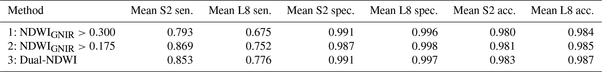
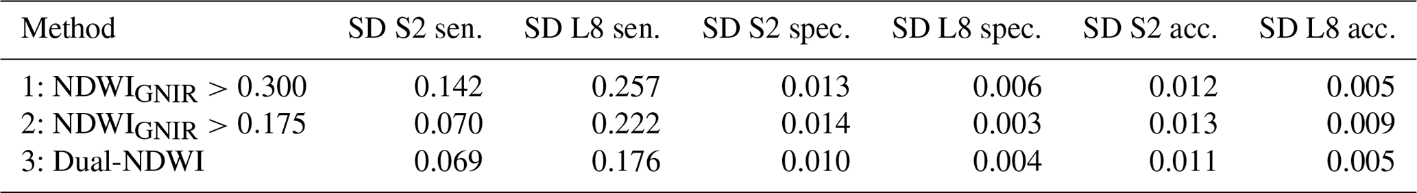
Table A2 Standard deviation (SD) of the values for sensitivity (sen.), specificity (spec.) and accuracy (acc.) across three test sites: Amery, George VI and Bach ice shelves for S2 and L8 Sensors.

Method 1 comprises a simple thresholding of NDWI_GNIR classification by excluding any pixels with an NDWI_GNIR value less than or equal to 0.300. This method was used to map lakes in January 2017 in East Antarctica and is the basis for three methods considered here. Method 2 utilised a lower threshold of 0.175 on NDWI_GNIR for more complete delineation of supraglacial hydrology. However, due to the lower threshold, more non-lake pixels were misclassified as lake pixels. To reduce such misclassifications, band filters were introduced to remove some cloud, rock, slush and shaded areas (Moussavi et al., 2020). Method 3 combines both NDWI classifications (NDWI_GNIR and NDWI_BR). A lower threshold of 0.16 is applied to the NDWI_GNIR classifier. In addition, the second classifier (NDWI_BR) was given a threshold of 0.18 (Moussavi et al., 2020). Additional band filters were applied in Method 3 as in Method 2.

As in the analysis in Sect. 2.2 “Accuracy assessment”, we compared the output of the three methods to the manually delineated lakes and channels. We computed the mean values for sensitivity, specificity and accuracy (Eqs. 5, 6 and 7) for each test site (Amery, George VI and Bach) across both sensors (S2 and L8) (Table A1). Based upon this assessment, the two best-performing methods are Methods 2 and 3. However, we selected the Dual-NDWI method because it performs well not only in terms of the average values but also in terms of the standard deviation for both sensors (Table A2). This indicates greater stability between sites, which is important when applying the method across other sites during the ice-sheet-wide roll-out.