the Creative Commons Attribution 4.0 License.
the Creative Commons Attribution 4.0 License.
 | 24 Mar 2022
Harmonized chronologies of a global late Quaternary pollen dataset (LegacyAge 1.0)
Chenzhi Li
Alexander K. Postl
Thomas Böhmer
Xianyong Cao
Andrew M. Dolman
Ulrike Herzschuh
We present a chronology framework named LegacyAge 1.0 containing harmonized chronologies for 2831 pollen records (downloaded from the Neotoma Paleoecology Database and the supplementary Asian datasets) together with their age control points and metadata in machine-readable data formats. All chronologies use the Bayesian framework implemented in Bacon version 2.5.3. Optimal parameter settings of priors (accumulation.shape, memory.strength, memory.mean, accumulation.rate, and thickness) were identified based on information in the original publication or iteratively after preliminary model inspection. The most common control points for the chronologies are radiocarbon dates (86.1 %), calibrated by the latest calibration curves (IntCal20 and SHCal20 for the terrestrial radiocarbon dates in the Northern Hemisphere and Southern Hemisphere and Marine20 for marine materials). The original publications were consulted when dealing with outliers and inconsistencies. Several major challenges when setting up the chronologies included the waterline issue (18.8 % of records), reservoir effect (4.9 %), and sediment deposition discontinuity (4.4 %). Finally, we numerically compare the LegacyAge 1.0 chronologies to those published in the original publications and show that the reliability of the chronologies of 95.4 % of records could be improved according to our assessment. Our chronology framework and revised chronologies provide the opportunity to make use of the ages and age uncertainties in synthesis studies of, for example, pollen-based vegetation and climate change. The LegacyAge 1.0 dataset, including metadata, datings, harmonized chronologies, and R code used, is open-access and available at PANGAEA (https://doi.org/10.1594/PANGAEA.933132; Li et al., 2021) and Zenodo (https://doi.org/10.5281/zenodo.5815192; Li et al., 2022), respectively.
- Article
(2864 KB) - Full-text XML
- BibTeX
- EndNote


Global and continental fossil pollen databases are used for a variety of paleoenvironmental studies, such as past climate and biome reconstructions, paleo-model validation, and the assessment of human–environmental interactions (Gajewski, 2008; Gaillard et al., 2010; Cao et al., 2013; Mauri et al., 2015; Trondman et al., 2015; Marsicek et al., 2018; Herzschuh et al., 2019). Several fossil pollen databases have been successfully established (Gajewski, 2008; Fyfe et al., 2009), such as the European Pollen Database (http://www.europeanpollendatabase.net/index.php, last access: 1 July 2020), the North American Pollen Database (https://www.ncei.noaa.gov/products/paleoclimatology, last access: 1 July 2020), and the Latin American Pollen Database (http://www.latinamericapollendb.com/, last access: 1 July 2020); most of these data are now included in the Neotoma Paleoecology Database (https://www.neotomadb.org/, last access: 1 April 2021; Williams et al., 2018). Chronologies and age control points are stored in these databases along with the pollen records.
However, to date, the metadata and dating results of these records are not available in a machine-readable format; furthermore, the chronologies have been established using a variety of methodologies, and the quantification of temporal uncertainty, particularly between records, remains a challenge (Blois et al., 2011; Giesecke et al., 2014; Flantua et al., 2016; Trachsel and Telford, 2017). Recently, the need for harmonized and consistent chronologies allowing for the accurate assessment of temporal uncertainty between records has increased as studies are looking for spatiotemporal patterns using multi-record analyses (Jennerjahn et al., 2004; Blaauw et al., 2007; Giesecke et al., 2011; Flantua et al., 2016). Accordingly, some effort has been made to harmonize the chronologies for a subset of the records in these databases (Fyfe et al., 2009; Blois et al., 2011; Giesecke et al., 2011, 2014; Flantua et al., 2016; Brewer et al., 2017; Wang et al., 2019; Mottl et al., 2021). However, a harmonized chronology framework is needed, not only to allow for the consistent inference of age and age uncertainties but also to apply to newly published records or one that can be adjusted to the specific requirement of a study.
Here we present the rationale and code, as well as the metadata and parameter settings, for the chronology framework LegacyAge 1.0, which contains harmonized chronologies for 2831 palynological records, synthesized from the Neotoma Paleoecology Database (Neotoma hereafter) and the supplementary Asian datasets (Cao et al., 2013, 2020). We also report on the major challenges of setting up the chronologies and assessing their quality. Finally, the newly harmonized chronologies are numerically compared with the original ones. All data and R code used for this study are open-access and available at PANGAEA (https://doi.org/10.1594/PANGAEA.933132; Li et al., 2021) and Zenodo (https://doi.org/10.5281/zenodo.5815192; Li et al., 2022), respectively.
2.1 Data sources
We established harmonized chronologies for 3471 records in a framework called LegacyAge 1.0. This compilation comprises 3147 records from Neotoma and 324 Asian records from China and Siberia compiled by Cao et al. (2013, 2020) and from our own data (AWI, Alfred Wegener Institute). Records are from lake sediments (49.4 %), peatlands (34.3 %), and other archives (16.3 %) (Fig. 1). The following chronology metadata were collected for each record: Event, Data_Source, Site_ID, Dataset_ID, Site_Name, Location (longitude, latitude, elevation, and continent), Archive_Type, Site_Description, Reference, Laboratory_Label, Dating_Method, Material_Dated, and Date (uncalibrated and calibrated age, error older, error younger, depth, and thickness), as well as additional relevant comments from authors (e.g., reservoir effect, hiatus, outliers, and date rejected). Furthermore, information on the original chronologies of each pollen record was also taken from the Neotoma and supplementary Asian datasets, including Chronology_Name, Age_Type (calibrated or uncalibrated radiocarbon years BP), Pollen_Depth, and Estimated_Age (age and age error). These metadata are available at https://doi.org/10.1594/PANGAEA.933132 (Tables S1 and S4 in Li et al., 2021).
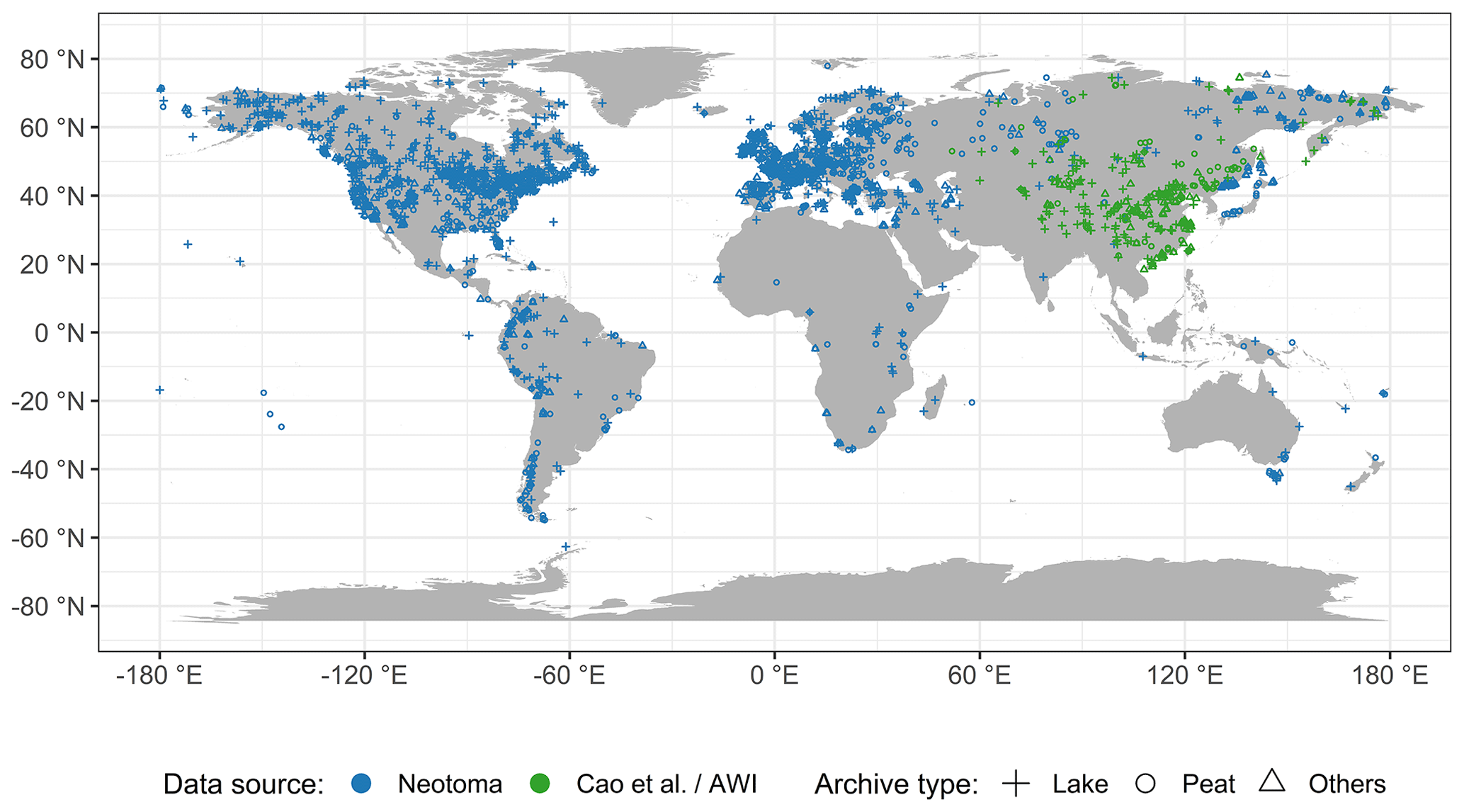
Figure 1Map of records by source and archive type.
2.2 Chronological control points
2.2.1 Radiometric dates
Radiocarbon dating. Most records were dated using radiocarbon-based methods (14C dating: conventional or accelerator mass spectrometry; Christie, 2018), covering the time range of ca. the last 50 kyr BP (before present, where “present” is 1950 CE). However, the accuracy and precision of the radiocarbon dates depend on the calibration curve, taphonomy, and dating materials (Blois et al., 2011; Heaton et al., 2021).
Lead-210 dating. The uppermost part of some lake records has been dated using a radioactive isotope of lead (lead-210), which has a half-life of ca. 22 years and provides useful age control for the last 75–150 years. However, the abundance of other radioactive isotopes (e.g., caesium-137) affects the accuracy and precision of the calibration curve for lead-210, resulting in temporal uncertainty (Appleby and Oldfield, 1978; Cuney, 2021).
Luminescence dating. Archeological materials, loess, and river sediments have often been dated via luminescence, including thermoluminescence (TL) and optically stimulated luminescence (OSL), which cover timescales from millennia to hundreds of thousands of years (Roberts, 2014). Due to the systematic and random errors in the measurement process, the luminescence ages have at least 4 %–5 % uncertainty, which widens with increasing time (Wallinga and Cunningham, 2014).
2.2.2 Lithological dates
Varve dating. Varve chronology, generated from counting varves, is considered a relatively accurate dating method for the late Quaternary, particularly the Holocene. Although sediment characteristics (e.g., thickness, continuity, and marking layer) may create uncertainty in varve-counted ages, these uncertainties are small relative to those from radiometric methods (Ojala et al., 2012; Zolitschka et al., 2015; Ramisch et al., 2020). If a pollen record has a varve chronology stored and assessed in the Varved Sediments Database (VARDA, https://varve.gfz-potsdam.de/, last access: 1 April 2021), we generally prefer to use it over chronologies based on other dating techniques.
Tephrochronology. Tephra layers are used as isochrones to correlate and synchronize sequences at a regional or continental scale (Lowe, 2011). The uncertainties of tephrochronology are similar to those known in radiocarbon dating, such as methodological and dating errors (Flantua et al., 2016). Tephras documented in the global Tephrochronological Database (Tephrabase, https://www.tephrabase.org/, last access: 1 April 2021) were included to improve the chronologies, such as the Mazama ash (7630±40 cal years BP; Brown and Hebda, 2003), Vedde ash (12 121±57 cal years BP; Lane et al., 2012), and the Laacher See ash (12 880±120 cal years BP).
2.2.3 Biostratigraphical dates
Biostratigraphical dates were widely relied on before 14C dating became available and affordable (Bardossy and Fodor, 2004). We ignored most of the available biostratigraphical dates when we harmonized the chronologies because vegetation reaction to climate change is likely not sufficiently synchronous. Only a few well-known and widely applicable biostratigraphic boundaries (Rasmussen et al., 2014) were used in other dating techniques that could not sufficiently constrain the chronologies, for example, the Younger Dryas–Holocene (11 500±250 cal years BP), Allerød–Younger Dryas (12 650±250 cal years BP), and Oldest Dryas–Bølling (14 650±250 cal years BP; Giesecke et al., 2014).
2.3 Establishing the chronologies
2.3.1 Method choice
We used the Bacon software (Blaauw and Christen, 2011) to establish continuous down-core chronologies from the age control points. Bacon fits a monotonic autoregressive (AR1) model to age control points using Bayesian methods to combine information from the control points with prior information on the statistical properties of accumulation histories for deposits, e.g., a prior distribution for the mean accumulation rate and how it varies (Blaauw and Christen, 2011). Several other approaches are available for age–depth modeling, including linear interpolation; smoothing splines; and other Bayesian methods, e.g., OxCal (Ramsey, 2008) and Bchron (Haslett and Parnell, 2008). However, Bacon has become one of the most frequently used and compares well with other methods (Trachsel and Telford, 2017; Blaauw et al., 2018).
Bacon provides the calibrated ages (mean, median, minimum, and maximum) at each depth (e.g., every centimeter) with 95 % confidence intervals and an indication of how well the model fits the dates, although it needs much supervision and computing power. The prior distribution guides the overall trend of the age–depth relationships, so the control points guide rather than strictly constrain the age–depth relationships (Giesecke et al., 2014). Bacon version 2.3.3 and later (Blaauw and Christen, 2011) can also handle sudden shifts in the accumulation rate when given the hiatus–boundary depth and resetting the memory to 0 when crossing the hiatus. Therefore, all age–depth relationships in our dataset will be constructed using the latest version of Bacon, 2.5.3 (Blaauw and Christen, 2011; Blaauw et al., 2018), in R (R Core Team, 2020).
2.3.2 Core tops and basal ages
Wherever possible, the record-related publications were read to decide whether the core top was modern at the time of sampling. For modern core tops, if the core was collected from sites where sediment was still accumulating, the sediment surface could be assigned to the year of sampling, adding one significant time control for the chronologies. If the sampling date was unavailable, an alternative surface age from the original chronology in Neotoma was added at the core top. An estimated artificial core top age ( cal years BP) was used if none of the above ages were available (Tables S2 and S3 in Li et al., 2021). We inferred the surface age from the calibrated age–depth model for core tops judged not to be modern. For basal ages, when the calibrated age–depth model for the lowermost profile has considerable extrapolation and was not sufficiently constrained by the control points; we also accepted the prior information of core basal age from the record-related publications or Neotoma.
2.3.3 Calibration curves
To transform the measured 14C ages to calendar ages, the latest calibration curves, approved by the radiocarbon community (Hajdas, 2014), were used in the Bacon routine: IntCal20 (Reimer et al., 2020; Heaton et al., 2021) and SHCal20 (Hogg et al., 2020) to calibrate the terrestrial radiocarbon dates in the Northern Hemisphere and Southern Hemisphere, respectively, and Marine20 (Heaton et al., 2020) for the 38 marine records included in our dataset (Sánchez Goñi et al., 2017). The numerical probability distributions of calendar age from calibrated radiocarbon dates were summarized to a mean and standard deviation for use in Bacon. Absolute dates (e.g., lead-210, OSL, and tephra), already presented on the calendar scale, were not calibrated (Blaauw and Christen, 2011). Modern/post-bomb 14C dates (negative 14C ages) were calibrated using appropriate post-bomb calibration curves (post-bomb: 1 for >40∘ N, 2 for 0–40∘ N, and 4 for Southern Hemisphere; Hua et al., 2013).
2.3.4 Parameter settings for the initial Bacon run
After consultation of the relevant publication (Blaauw and Christen, 2011; Goring et al., 2012; Cao et al., 2013; Fiałkiewicz-Kozieł et al., 2014; Blaauw et al., 2018) and assessments of several runs with a test set of records, we set the following Bacon parameters (Table S3 in Li et al., 2021):
-
The prior for the accumulation rate consists of a gamma distribution with two parameters, mean accumulation rate (acc.mean; default 20 yr cm−1) and accumulation shape (acc.shape; default 1.5). For the acc.shape, we accepted its default value, as higher values resulted in a more peaked shape of the gamma distribution. A first approximation of the acc.mean was calculated as the average accumulation rate between the first and the last date of each record, combined with the prior information of dates, which is more reasonable than using a constant value.
-
Bacon divides a core into many vertical sections of equal thickness (thick; default 5 cm), which significantly affects the flexibility of the age–depth model, and through millions of Markov chain Monte Carlo iterations estimates the accumulation rate for each section. Blaauw and Christen (2011) indicated that models with few sections tend to show more abrupt changes in accumulation rate, while models with many sections usually appear smoother but are computationally more intense. We run Bacon for six section thicknesses (2.5, 5, and 10 cm; 30, 60, and 120 sections), optimal values after numerous tests, and with and without core top age resulting in 12 initial chronologies for each record.
-
The prior for the memory, that is, the dependence of accumulation rate between neighboring depths, is a beta distribution defined by two parameters: memory strength (mem.strength; default 10) and mean memory (mem.mean; default 0.5). For the mem.strength, we used a value of 20 as suggested by Goring et al. (2012), which allows for a large range of posterior memory values. We set different mem.mean values (0.3 for lake and 0.7 for peatland) to accommodate differences in accumulation conditions between lakes and peatland, where the higher memory for peatlands implies a more constant accumulation history (Blaauw and Christen, 2011; Goring et al., 2012; Cao et al., 2013, 2020).
-
The minimum (maximum) depth (d.min and d.max, respectively) of the age–depth model was defined by the uppermost (lowermost) dating or pollen sample depth (Table S4 in Li et al., 2021). The parameter “d.by” (default 1 cm) defines the depth intervals at which ages are calculated, and we accepted its default value.
In addition to the major parameters mentioned above, we also adjusted several additional parameters for individual records according to prior information collected from record-related publications or Neotoma (Tables S2 and S3 in Li et al. 2021).
-
Reservoir effects. The uptake of old carbon by aquatic plants, mosses, or shells either originating from, e.g., limestone in the catchment (“hard-water effect”) or slow 14C exchange between the atmosphere and ocean interior can result in radiocarbon dates which are too old (Philippsen, 2013; Philippsen and Heinemeier, 2013; Giesecke et al., 2014; Heaton et al., 2020). In addition to the reservoir ages reported by the original authors, we identified some other records that may be affected by a reservoir effect. In that case – and only for records from sites where sediment was still accumulating – we applied modern correction and linear extrapolation (Hou et al., 2012; Wang et al., 2017) to infer the reservoir age. We then subtracted the reservoir age as a constant from all 14C dates of an affected record, excluding those derived from terrestrial macrofossils. We may have underestimated the number of such records due to the difficulty of estimating the reservoir age where the sediment surface was eroded or used for agricultural purposes.
-
Waterline issues. Stratigraphic records do not always start at a depth of 0 cm, for example; if the uppermost part of the core is lost; if the record is only a part of a longer sequence; or if the depths are measured from the water surface instead of the sediment surface, leading to the so-called waterline issue. Accordingly, we adjusted the uppermost depth of the chronology based on information collected from the original publications and Neotoma.
-
Hiatuses. Where sediment deposition was not continuous, it is possible to set a “hiatus” at which Bacon resets the memory to 0, causing a break in the autocorrelation in the accumulation rate for depths before and after the hiatus and additionally models an instantaneous jump in age at that depth (Blaauw and Christen, 2011).
-
Dates rejected/added. Neotoma usually reports all 14C dates from cores, even when deemed inaccurate. We assessed prior information on dates and then excluded the 14C dates of samples with contaminated or reworked sediments from age–depth models, in most cases following the suggestions in the original publications. For example, we excluded the date at 164 cm, accepted by the author (Gajewski et al., 2000), from the Muskox Lake record (Dataset_ID 1783), as it does not agree with the other three dates from the same core and where lithology had changed significantly at that depth. We down-weighted the impact of outliers on the overall trend of the age–depth relationships and risked that age uncertainties were too optimistic. To supplement the chronology metadata, we also documented all lithological dates (e.g., varves and tephra) and biostratigraphical dates collected from the original publications and Neotoma.
2.3.5 Assessment of initial age–depth models and final parameter selection
To objectively evaluate the 12 initial age–depth models for each record, we initially tested a least-squares method between the age model and ages of dated depths and calculated the mean uncertainty for each model. However, the least-squares method is susceptible to outliers (Birks et al., 2012), and models with least squares may risk more abrupt changes in accumulation rate due to overfitting dates. Instead of a numerical comparison, we finally implemented a visual comparison based on the Bacon output graphs, which show the Markov chain Monte Carlo iterations, the prior and posterior distributions for the accumulation rate and memory, and how well the model fits the date (Blaauw and Christen, 2011).
Preference was given to models that fitted the dates well, had small mean uncertainties (Table S5 in Li et al., 2021), and good runs of Markov chain Monte Carlo iterations (i.e., a stationary distribution with little structure among neighboring iterations as indicated by the trace plot of the joint likelihood) when visual choosing the “best” model for each record (Blaauw and Christen, 2011; Blaauw et al., 2018). If necessary, we adjusted the parameter settings such as the section thickness and mean accumulation rate to better fit the dates consistent with prior information. For the final parameter settings used for each record, please see https://doi.org/10.1594/PANGAEA.933132 (Table S3 in Li et al., 2021).
2.4 Evaluation of the newly generated age–depth models
For the temporal uncertainty of the age–depth models, we take used the 95 % confidence intervals for age estimated by the Bacon model for each centimeter (Table S5 in Li et al., 2021). These values are approximately twice the standard error of the estimated age at a given depth. We plotted our newly generated “best” calibrated chronologies with 95 % confidence intervals together with the original ones taken from the Neotoma and Cao et al. (2013, 2020) datasets (Table S4 in Li et al., 2021) to compare and evaluate the performance of the new models visually. The criteria for the preferred models are that the model fitted the dates well, had small uncertainties, combined dates with prior information (e.g., geological and hydrological setting and environmental history), and calibrated with the latest calibration curves.
3.1 Overview of major challenges when establishing the chronologies
Age–depth models were initially established for all 3471 records in the harmonized pollen data collection (Herzschuh et al., 2021). We discarded 640 records with fewer than two reliable dates (i.e., no reliable date or only one reliable date), evaluated based on prior information from the original literature, leaving chronologies for 2831 records. We faced several major challenges when establishing the chronologies. After assessments and consultation of prior information from original publications (Tables S2 and S3 in Li et al. 2021), we identified 139 records (4.9 %) with reservoir effects, 533 records (18.8 %) with waterline issues, 125 records (4.4 %) with hiatuses, 924 records (32.6 %) with rejected or added dates, and 743 records (26.2 %) that contained several of the above problems; all these challenges have been handled (Fig. 2). After assessing initial age–depth models, accumulation rates were adjusted for 367 records (13.0 %), and different section thicknesses were applied to 411 records (14.5 %).
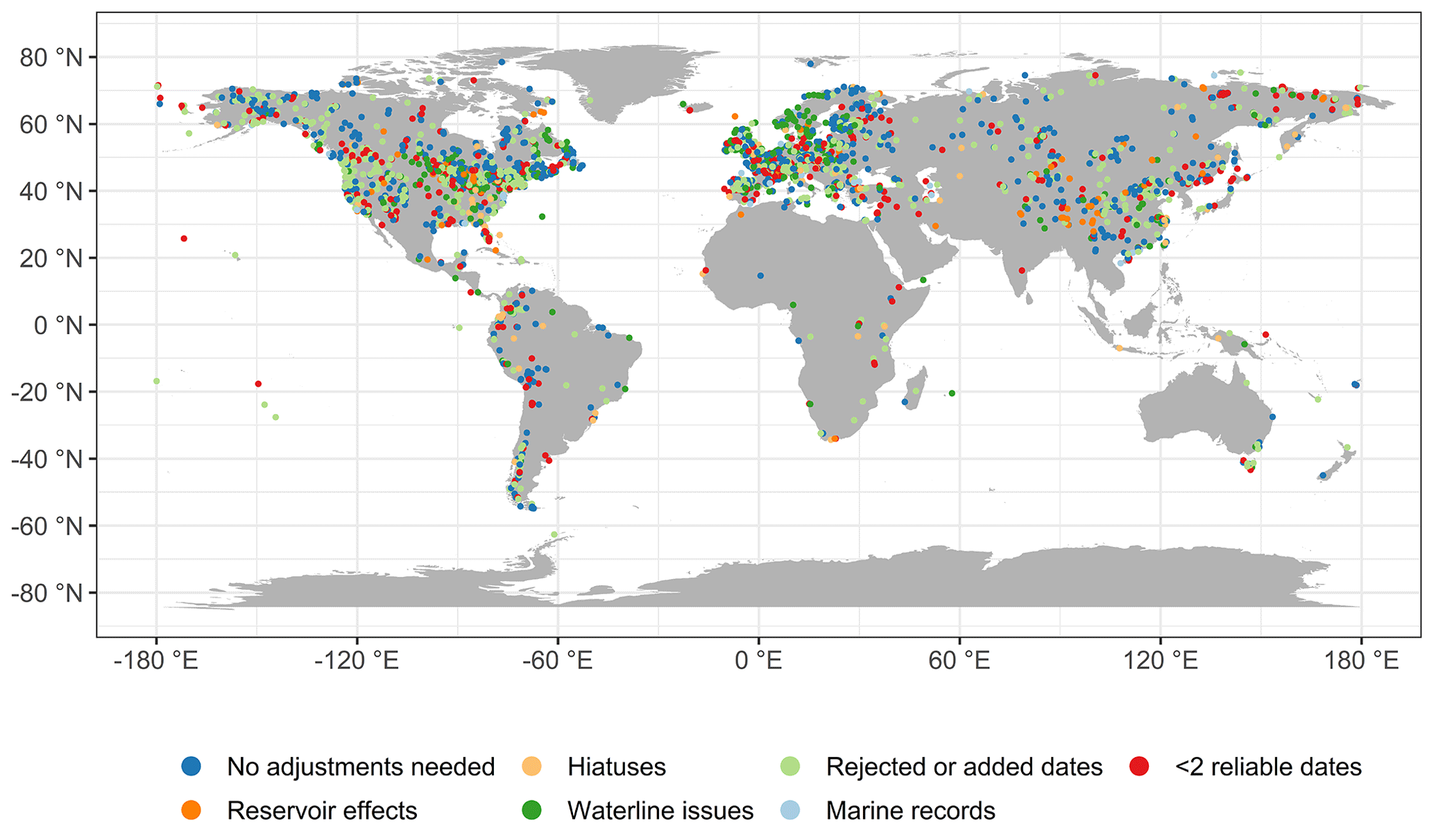
Figure 2The distribution of records that faced various major challenges when establishing their chronologies.
3.2 LegacyAge 1.0 quality
3.2.1 Dates used for final chronologies
A total of 19 990 control points (out of 21 199 dates available) were used to generate the chronologies for the 2831 records (Table S1 in Li et al., 2021). Among them, the most common chronological control points are radiocarbon dates (86.1 %), followed by lithological and biostratigraphical dates (8.5 %) collected from publications or Neotoma, and lead-210 (5.0 %); other dating techniques make up 0.4 % of the control points. The median number of dates per chronology is 5, with 23.3 % of the chronologies having two or three dates, 53.3 % having four to eight dates, and 23.4 % having at least nine dates (Fig. 3).
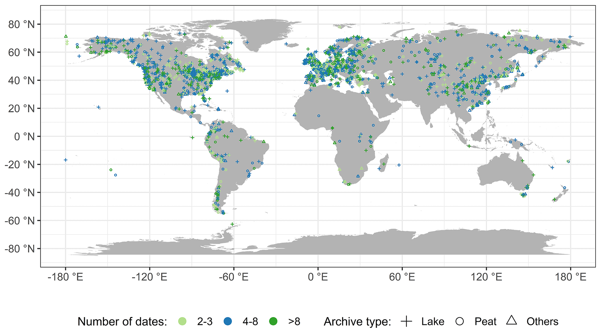
Figure 3Map of the number of dates and archive types for each record.
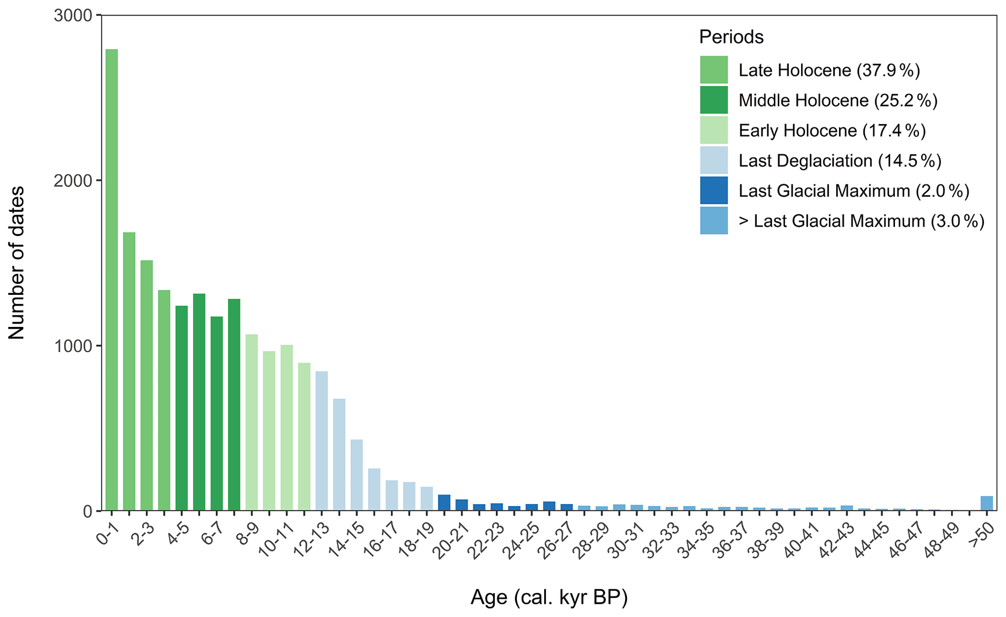
Currently, 80.5 % of chronological control points in the LegacyAge 1.0 fall within the Holocene (37.9 %, 25.2 %, and 17.4 % within the Late (ca. 0–4.2 cal kyr BP), Middle (ca. 4.2–8.2 cal kyr BP), and Early Holocene (ca. 8.2–11.7 cal kyr BP), respectively), 14.5 % within the last deglaciation (ca. 11.7–19.0 cal kyr BP; Clark et al., 2012), 2.0 % within the Last Glacial Maximum (LGM; ca. 19.0–26.5 cal kyr BP; Clark et al., 2009), and only 3.0 % earlier than the LGM (Fig. 4).
3.2.2 Spatial and temporal coverage
Of the 2831 chronologies finally established, 1032 records are from North America, 1075 from Europe, 488 from Asia, 150 from South America, 54 from Africa, and 32 from the Indo-Pacific (Fig. 3). Most records (2659 records, 93.9 %) are in the Northern Hemisphere, where the main vegetation and climate zones are covered.
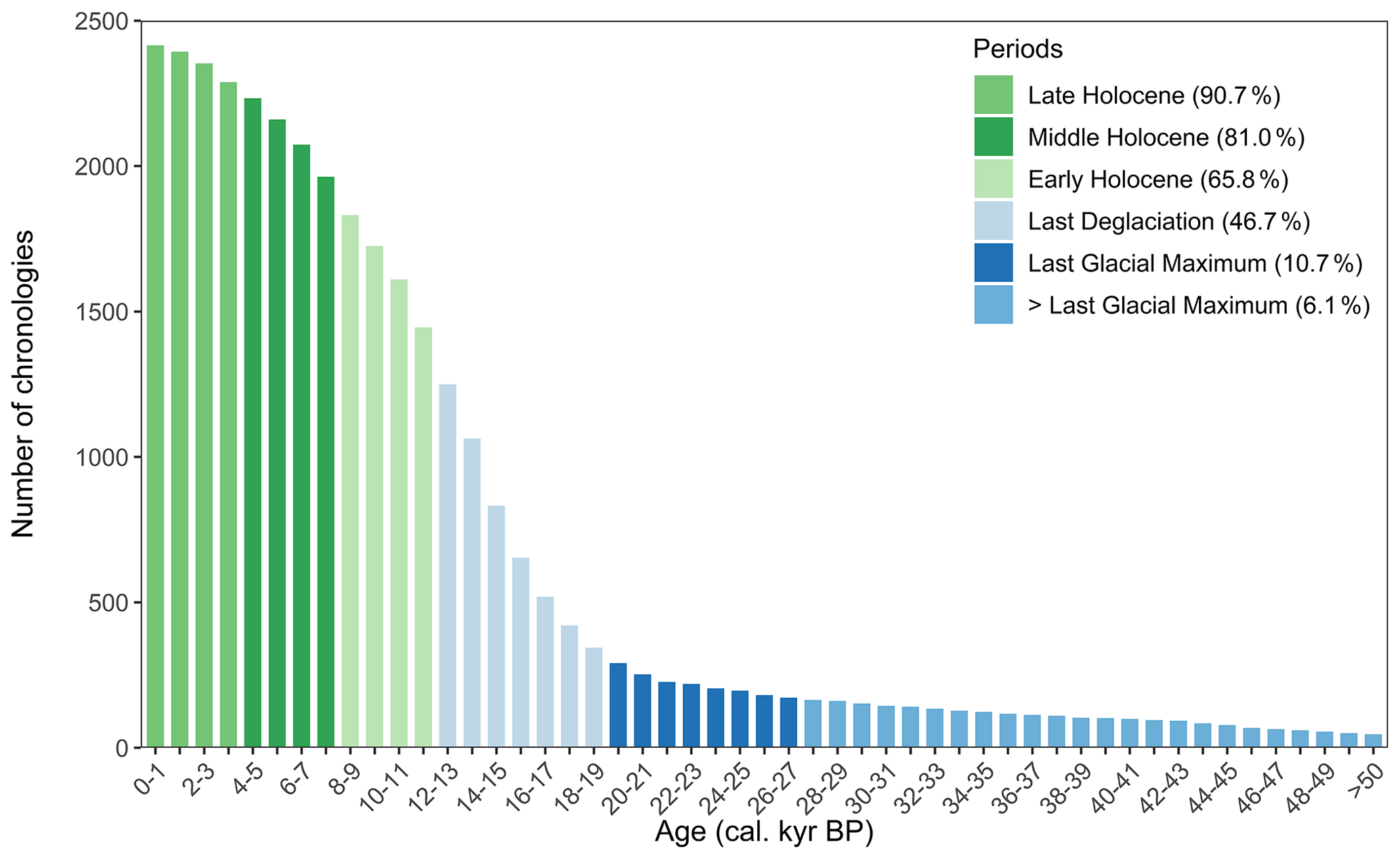
As shown in Fig. 5, 94.8 % of chronologies cover part of the last 30 kyr, while Marine Isotope Stage 3 (MIS 3) is relatively poorly covered. Specifically, 98.0 % of chronologies cover part of the Holocene (90.7 %, 81.0 %, and 65.8 % cover part of the Late, Middle, and Early Holocene, respectively); 46.7 % cover part of the Last Deglaciation; 10.7 % cover part of the Last Glacial Maximum; and only 6.1 % are from earlier than the LGM.
3.2.3 Temporal uncertainty
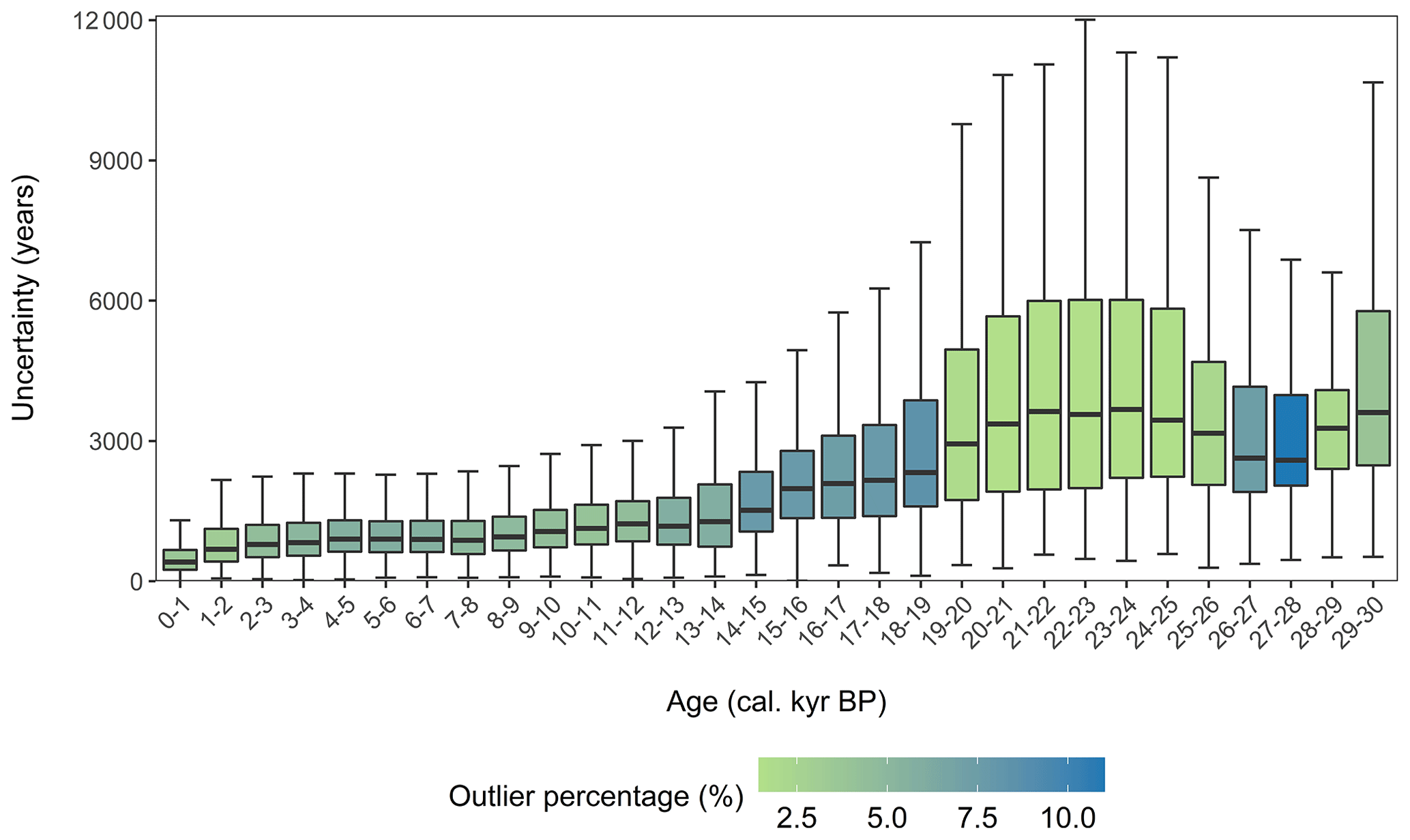
Boxplots of age uncertainties for all chronologies in distinct time slices (Fig. 6), excluding outliers (ca. 5.1 %), illustrate that age uncertainty tends to increase with age and is mainly related to the uncertainty and precision of the chronological control points, calibration curves, and age models (Blois et al., 2011). The boxplots show wide boxes, i.e., a more extensive data range, for the LGM period, characterized by fewer outliers, mostly from chronologies with sparse age control points and significant dating errors, than the periods with small box sizes.
3.3 Comparison of the LegacyAge 1.0 vs. original age–depth models
For 906 records out of the 2831 records included in the LegacyAge 1.0, no calibrated chronologies were originally available from the Neotoma and Cao et al. (2013, 2020) datasets for comparison. Of the remaining 1925 records, the new LegacyAge 1.0 chronologies were selected instead of the original ones in 95.4 % of cases, based on the aforementioned criteria. However, some records still chose the original chronology, mainly because they are varve chronologies, had incomplete metadata (e.g., missing sample depths), or included some non-14C dates that our model could not accommodate (Table S6 in Li et al., 2021).
In most cases, the newly established chronologies were rather similar to the original ones. For 1012 records (52.6 % of 1925 records), the original chronologies were within the 95 % confidence intervals of the LegacyAge 1.0 chronologies, while the other 913 records (47.4 %) were partially or completely outside the 95 % confidence intervals.
Selected typical examples of the comparative results between the accepted LegacyAge 1.0 chronologies, alternative newly generated but rejected chronologies, and the original chronologies are illustrated in Fig. 7. For the El Tiro Pass record (Dataset_ID 47502, Fig. 7a), both the original and LegacyAge 1.0 chronologies were established by Bacon and are acceptable. However, the LegacyAge 1.0 chronology has the advantage that it makes use of the latest radiocarbon calibration curve (IntCal20; Reimer et al., 2020), and the estimated surface age is more realistic as sediments are still accumulating (Niemann and Behling, 2008). For the Fargher Pond record (Dataset_ID 15344, Fig. 7b), the LegacyAge 1.0 chronology includes more varve ages from the Varved Sediments Database. These provide a better constraint for the lowermost profile than the original model had (Grigg and Whitlock, 2002). For the Oltush Lake record (Dataset_ID 4320, Fig. 7c), the 14C age of modern sediment in this lake is 350 years BP, and thus, the assumption of a reservoir effect of 350 years resulted in slightly younger ages than originally given (Davydova and Servant-Vildary, 1996). Some alternative rejected chronologies performed poorly due to the inability of high-resolution Bacon models to accommodate accumulation rate changes (Fig. 7b and c). Finally, for the Soppensee record (Dataset_ID 44723, Fig. 7d), most of the 14C dates (>540 cm) come from samples with insufficient carbon to achieve accurate dating (Hajdas and Michczyński, 2010), and thus the original chronology, generated from counting varves, outperformed our newly generated chronologies.
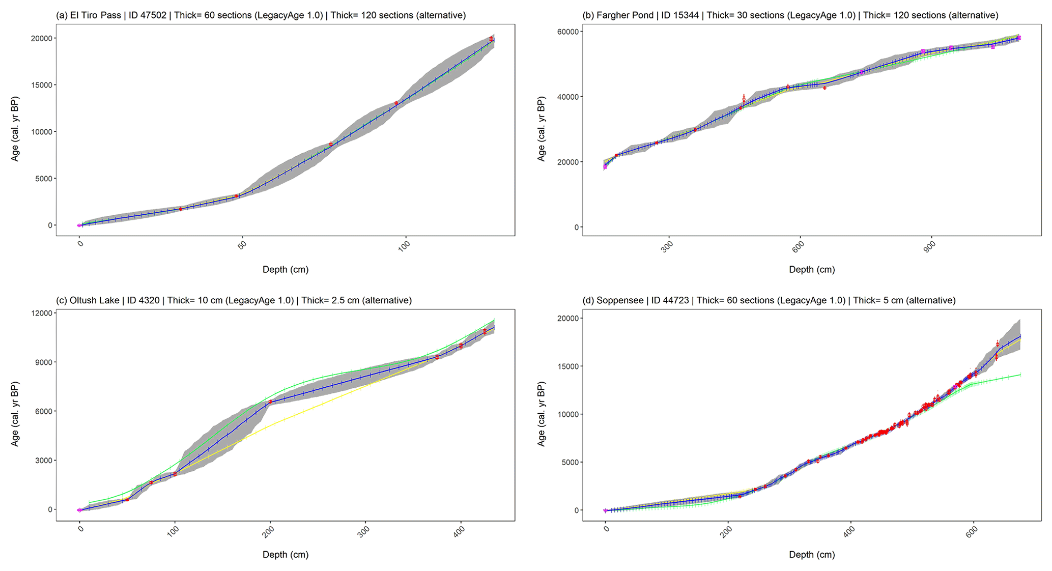
Figure 7Comparison of LegacyAge 1.0 chronologies with the original ones. Green line: original chronology. Blue line: LegacyAge 1.0 chronology. Yellow line: alternative newly generated but rejected chronology. Red: date in chronology metadata. Pink: date from prior information. Grey shading: age uncertainties (95 % confidence intervals).
Seven supplementary datasets (Tables S1–S7, in comma-separated values format) and one readme text about the LegacyAge 1.0 are accessible in the navigation bar “Further details” of the PANGAEA page (https://doi.org/10.1594/PANGAEA.933132; Li et al., 2021). We provided the metadata of the chronological control points (Table S1), prior information of dates from publication (Table S2), Bacon parameter settings (Table S3), original chronology metadata from the Neotoma and Cao et al. (2013, https://doi.org/10.1016/j.revpalbo.2013.02.003; 2020, https://doi.org/10.5194/essd-12-119-2020) (Table S4), LegacyAge 1.0 chronology (Table S5), description of the comparison of original chronology and LegacyAge 1.0 (Table S6), and record references (Table S7), respectively. All datasets are already in long data format that can be joined by the dataset ID.
The R code for calculation and comparison of chronologies with an embedded manual, metadata for code runs, Bacon output graphs of each record, graph comparison of original chronologies and LegacyAge 1.0, and a short shared-screen video of the R code to show the usage on two example records are accessible on Zenodo (https://doi.org/10.5281/zenodo.5815192; Li et al., 2022).
LegacyAge 1.0 provides the calibrated ages (mean, median, minimum, and maximum) and uncertainties at each centimeter for each record with a 95 % confidence interval (Table S5 in Li et al., 2021). All users can apply some interpolation algorithms in the chronologies, subsetted from the LegacyAge 1.0 dataset or outputted by our code, to assign ages for proxy depths of records.
As for the R code, users only need to set the working directory where the Bacon results will be stored and input the record ID of interest to run it successfully. The manual and shared-screen video on R code usage could provide helpful guidance for users, with or without some R experience.
This paper presents the framework as well as metadata, machine-readable datings, R pipeline, chronologies, and age uncertainties of 2831 pollen records synthesized from the Neotoma Paleoecology Database and the supplementary Asian datasets (Cao et al., 2013, 2020). Chronologies and uncertainties can be used for synthesis works; metadata, datings, and pipelines can be used to re-establish the chronologies for customized purposes, and the framework can be used to establish chronologies for newly updated records.
UH and CL designed the chronology dataset. CL and TB compiled the metadata and prior information of the chronologies. AKP and TB wrote the R scripts and ran the analyses under the supervision of UH and CL. AMD contributed an initial R script for creating age–depth models with Bacon. XC helped in the collection of Asian pollen records. CL wrote the first draft of the manuscript under the supervision of UH. All authors discussed the results and contributed to the final manuscript.
The contact author has declared that neither they nor their co-authors have any competing interests.
Publisher’s note: Copernicus Publications remains neutral with regard to jurisdictional claims in published maps and institutional affiliations.
The majority of data were obtained from the Neotoma Paleoecology Database (https://www.neotomadb.org/, last access: 1 April 2021). The work of data contributors, data stewards, and the Neotoma community is gratefully acknowledged. We would like to express our gratitude to all the palynologists and geologists who, either directly or indirectly, contributed pollen data and chronologies to the dataset. We thank Andrej Andreev, Mareike Wieczorek, and Birgit Heim from AWI for providing information on pollen records and data uploads. We also thank Cathy Jenks for language edits to a previous version of the paper. This study was undertaken as part of LandCover6k, a working group of Past Global Changes (PAGES), which in turn received support from the US National Science Foundation, the Swiss National Science Foundation, the Swiss Academy of Sciences, and the Chinese Academy of Sciences.
This research has been supported by the European Research Council, H2020 European Research Council (GlacialLegacy; grant no. 772852 to Ulrike Herzschuh), the Bundesministerium für Bildung und Forschung (grant no. 01LP1510C to Ulrike Herzschuh), and the China Scholarship Council (grant no. 201908130165 to Chenzhi Li).
This paper was edited by Jens Klump and reviewed by three anonymous referees.
Appleby, P. G. and Oldfield, F.: The calculation of lead-210 dates assuming a constant rate of supply of unsupported 210Pb to the sediment, Catena, 5, 1–8, https://doi.org/10.1016/S0341-8162(78)80002-2, 1978.
Bardossy, G. and Fodor, J.: Evaluation of Uncertainties and Risks in Geology: New Mathematical Approaches for Their Handling, Springer Science & Business Media, 250 pp., ISBN-13: 978-3-540-20622-4 (ISBN-10: 3-540-20622-1), 2004.
Birks, H. J. B., Lotter, A. F., Juggins, S., and Smol, J. P.: Tracking Environmental Change Using Lake Sediments: Data Handling and Numerical Techniques, Springer Science & Business Media, 751 pp., https://doi.org/10.1007/978-94-007-2745-8, 2012.
Blaauw, M. and Christen, J. A.: Flexible paleoclimate age-depth models using an autoregressive gamma process, Bayesian Anal., 6, 457–474, https://doi.org/10.1214/11-BA618, 2011.
Blaauw, M., Christen, J. A., Mauquoy, D., van der Plicht, J., and Bennett, K. D.: Testing the timing of radiocarbon-dated events between proxy archives, Holocene, 17, 283–288, https://doi.org/10.1177/0959683607075857, 2007.
Blaauw, M., Christen, J. A., Bennett, K. D., and Reimer, P. J.: Double the dates and go for Bayes – Impacts of model choice, dating density and quality on chronologies, Quaternary Sci. Rev., 188, 58–66, https://doi.org/10.1016/j.quascirev.2018.03.032, 2018.
Blois, J. L., Williams, J. W. J., Grimm, E. C., Jackson, S. T., and Graham, R. W.: A methodological framework for assessing and reducing temporal uncertainty in paleovegetation mapping from late-Quaternary pollen records, Quaternary Sci. Rev., 30, 1926–1939, https://doi.org/10.1016/j.quascirev.2011.04.017, 2011.
Brewer, S., Giesecke, T., Davis, B. A. S., Finsinger, W., Wolters, S., Binney, H., Beaulieu, J.-L. de, Fyfe, R., Gil-Romera, G., Kühl, N., Kuneš, P., Leydet, M., and Bradshaw, R. H.: Late-glacial and Holocene European pollen data, J. Maps, 13, 921–928, https://doi.org/10.1080/17445647.2016.1197613, 2017.
Brown, K. J. and Hebda, R. J.: Coastal rainforest connections disclosed through a Late Quaternary vegetation, climate, and fire history investigation from the Mountain Hemlock Zone on southern Vancouver Island, British Colombia, Canada, Rev. Palaeobot. Palyno., 123, 247–269, https://doi.org/10.1016/S0034-6667(02)00195-1, 2003.
Cao, X., Ni, J., Herzschuh, U., Wang, Y., and Zhao, Y.: A late Quaternary pollen dataset from eastern continental Asia for vegetation and climate reconstructions: Set up and evaluation, Rev. Palaeobot. Palyno., 194, 21–37, https://doi.org/10.1016/j.revpalbo.2013.02.003, 2013.
Cao, X., Tian, F., Andreev, A., Anderson, P. M., Lozhkin, A. V., Bezrukova, E., Ni, J., Rudaya, N., Stobbe, A., Wieczorek, M., and Herzschuh, U.: A taxonomically harmonized and temporally standardized fossil pollen dataset from Siberia covering the last 40 kyr, Earth Syst. Sci. Data, 12, 119–135, https://doi.org/10.5194/essd-12-119-2020, 2020.
Christie, M.: Radiocarbon dating, Wikij. Sci., 1, 1–17, https://doi.org/10.15347/WJS/2018.006, 2018.
Clark, P. U., Dyke, A. S., Shakun, J. D., Carlson, A. E., Clark, J., Wohlfarth, B., Mitrovica, J. X., Hostetler, S. W., and McCabe, A. M.: The Last Glacial Maximum, Science, 325, 710–714, https://doi.org/10.1126/science.1172873, 2009.
Clark, P. U., Shakun, J. D., Baker, P. A., Bartlein, P. J., Brewer, S., Brook, E., Carlson, A. E., Cheng, H., Kaufman, D. S., Liu, Z., Marchitto, T. M., Mix, A. C., Morrill, C., Otto-Bliesner, B. L., Pahnke, K., Russell, J. M., Whitlock, C., Adkins, J. F., Blois, J. L., Clark, J., Colman, S. M., Curry, W. B., Flower, B. P., He, F., Johnson, T. C., Lynch-Stieglitz, J., Markgraf, V., McManus, J., Mitrovica, J. X., Moreno, P. I., and Williams, J. W.: Global climate evolution during the last deglaciation, P. Natl. Acad. Sci. USA, 109, E1134–E1142, https://doi.org/10.1073/pnas.1116619109, 2012.
Cuney, M.: Nuclear Geology, in: Encyclopedia of Geology, 2nd edn., edited by: Alderton, D. and Elias, S. A., Academic Press, Oxford, 723–744, https://doi.org/10.1016/B978-0-08-102908-4.00024-2, 2021.
Davydova, N. and Servant-Vildary, S.: Late Pleistocene and Holocene history of the lakes in the Kola Peninsula, Karelia and the North-Western part of the East European plain, Quaternary Sci. Rev., 15, 997–1012, https://doi.org/10.1016/S0277-3791(96)00029-7, 1996.
Fiałkiewicz-Kozieł, B., Kołaczek, P., Piotrowska, N., Michczyński, A., Łokas, E., Wachniew, P., Woszczyk, M., and Sensuła, B.: High-Resolution Age-Depth Model of a Peat Bog in Poland as an Important Basis for Paleoenvironmental Studies, Radiocarbon, 56, 109–125, https://doi.org/10.2458/56.16467, 2014.
Flantua, S. G. A., Blaauw, M., and Hooghiemstra, H.: Geochronological database and classification system for age uncertainties in Neotropical pollen records, Clim. Past, 12, 387–414, https://doi.org/10.5194/cp-12-387-2016, 2016.
Fyfe, R. M., de Beaulieu, J. L., Binney, H., Bradshaw, R. H. W., Brewer, S., Le Flao, A., Finsinger, W., Gaillard, M. J., Giesecke, T., Gil-Romera, G., Grimm, E. C., Huntley, B., Kunes, P., Kühl, N., Leydet, M., Lotter, A. F., Tarasov, P. E., and Tonkov, S.: The European Pollen Database: past efforts and current activities, Veg. Hist. Archaeobot., 18, 417–424, https://doi.org/10.1007/s00334-009-0215-9, 2009.
Gaillard, M.-J., Sugita, S., Mazier, F., Trondman, A.-K., Broström, A., Hickler, T., Kaplan, J. O., Kjellström, E., Kokfelt, U., Kuneš, P., Lemmen, C., Miller, P., Olofsson, J., Poska, A., Rundgren, M., Smith, B., Strandberg, G., Fyfe, R., Nielsen, A. B., Alenius, T., Balakauskas, L., Barnekow, L., Birks, H. J. B., Bjune, A., Björkman, L., Giesecke, T., Hjelle, K., Kalnina, L., Kangur, M., van der Knaap, W. O., Koff, T., Lagerås, P., Latałowa, M., Leydet, M., Lechterbeck, J., Lindbladh, M., Odgaard, B., Peglar, S., Segerström, U., von Stedingk, H., and Seppä, H.: Holocene land-cover reconstructions for studies on land cover-climate feedbacks, Clim. Past, 6, 483–499, https://doi.org/10.5194/cp-6-483-2010, 2010.
Gajewski, K.: The Global Pollen Database in biogeographical and palaeoclimatic studies, Prog. Phys. Geog., 32, 379–402, https://doi.org/10.1177/0309133308096029, 2008.
Gajewski, K., Mott, R. J., Ritchie, J. C., and Hadden, K.: Holocene vegetation history of Banks Island, Northwest Territories, Canada, Can. J. Botany, 78, 430–436, https://doi.org/10.1139/b00-018, 2000.
Giesecke, T., Bennett, K. D., Birks, H. J. B., Bjune, A. E., Bozilova, E., Feurdean, A., Finsinger, W., Froyd, C., Pokorný, P., Rösch, M., Seppä, H., Tonkov, S., Valsecchi, V., and Wolters, S.: The pace of Holocene vegetation change – testing for synchronous developments, Quaternary Sci. Rev., 30, 2805–2814, https://doi.org/10.1016/j.quascirev.2011.06.014, 2011.
Giesecke, T., Davis, B., Brewer, S., Finsinger, W., Wolters, S., Blaauw, M., de Beaulieu, J.-L., Binney, H., Fyfe, R. M., Gaillard, M.-J., Gil-Romera, G., van der Knaap, W. O., Kuneš, P., Kühl, N., van Leeuwen, J. F. N., Leydet, M., Lotter, A. F., Ortu, E., Semmler, M., and Bradshaw, R. H. W.: Towards mapping the late Quaternary vegetation change of Europe, Veg. Hist. Archaeobot., 23, 75–86, https://doi.org/10.1007/s00334-012-0390-y, 2014.
Goring, S., Williams, J. W., Blois, J. L., Jackson, S. T., Paciorek, C. J., Booth, R. K., Marlon, J. R., Blaauw, M., and Christen, J. A.: Deposition times in the northeastern United States during the Holocene: establishing valid priors for Bayesian age models, Quaternary Sci. Rev., 48, 54–60, https://doi.org/10.1016/j.quascirev.2012.05.019, 2012.
Grigg, L. D. and Whitlock, C.: Patterns and causes of millennial-scale climate change in the Pacific Northwest during Marine Isotope Stages 2 and 3, Quaternary Sci. Rev., 21, 2067–2083, https://doi.org/10.1016/S0277-3791(02)00017-3, 2002.
Hajdas, I.: 14.3 – Radiocarbon: Calibration to Absolute Time Scale, in: Treatise on Geochemistry (Second Edition), edited by: Holland, H. D. and Turekian, K. K., Elsevier, Oxford, 37–43, https://doi.org/10.1016/B978-0-08-095975-7.01204-3, 2014.
Hajdas, I. and Michczyński, A.: Age-Depth Model of Lake Soppensee (Switzerland) Based on the High-Resolution 14C Chronology Compared with Varve Chronology, Radiocarbon, 52, 1027–1040, https://doi.org/10.1017/S0033822200046117, 2010.
Haslett, J. and Parnell, A.: A simple monotone process with application to radiocarbon-dated depth chronologies, J. R. Stat. Soc. C-Appl., 57, 399–418, https://doi.org/10.1111/j.1467-9876.2008.00623.x, 2008.
Heaton, T. J., Köhler, P., Butzin, M., Bard, E., Reimer, R. W., Austin, W. E. N., Ramsey, C. B., Grootes, P. M., Hughen, K. A., Kromer, B., Reimer, P. J., Adkins, J., Burke, A., Cook, M. S., Olsen, J., and Skinner, L. C.: Marine20–the marine radiocarbon age calibration curve (0–55,000 cal BP), Radiocarbon, 62, 779–820, https://doi.org/10.1017/RDC.2020.68, 2020.
Heaton, T. J., Bard, E., Bronk Ramsey, C., Butzin, M., Köhler, P., Muscheler, R., Reimer, P. J., and Wacker, L.: Radiocarbon: A key tracer for studying Earth's dynamo, climate system, carbon cycle, and Sun, Science, 374, eabd7096, https://doi.org/10.1126/science.abd7096, 2021.
Herzschuh, U., Cao, X., Laepple, T., Dallmeyer, A., Telford, R. J., Ni, J., Chen, F., Kong, Z., Liu, G., Liu, K.-B., Liu, X., Stebich, M., Tang, L., Tian, F., Wang, Y., Wischnewski, J., Xu, Q., Yan, S., Yang, Z., Yu, G., Zhang, Y., Zhao, Y., and Zheng, Z.: Position and orientation of the westerly jet determined Holocene rainfall patterns in China, Nat. Commun., 10, 2376, https://doi.org/10.1038/s41467-019-09866-8, 2019.
Hogg, A. G., Heaton, T. J., Hua, Q., Palmer, J. G., Turney, C. S., Southon, J., Bayliss, A., Blackwell, P. G., Boswijk, G., Ramsey, C. B., Pearson, C., Petchey, F., Reimer, P., Reimer, R., and Wacker, L.: SHCal20 Southern Hemisphere calibration, 0–55,000 years cal BP, Radiocarbon, 62, 759–778, https://doi.org/10.1017/RDC.2020.59, 2020.
Hou, J., William, J. D. A., and Liu, Z.: Geochronological limitations for interpreting the paleoclimatic history of the Tibetan Plateau, Quaternary Sciences, 32, 441–453, https://doi.org/10.3969/j.issn.1001-7410.2012.03.10, 2012 (in Chinese with English abstract).
Hua, Q., Barbetti, M., and Rakowski, A. Z.: Atmospheric radiocarbon for the period 1950–2010, Radiocarbon, 55, 2059–2072, https://doi.org/10.2458/azu_js_rc.v55i2.16177, 2013.
Jennerjahn, T. C., Ittekkot, V., Arz, H. W., Behling, H., Pätzold, J., and Wefer, G.: Asynchronous Terrestrial and Marine Signals of Climate Change During Heinrich Events, Science, 306, 2236–2239, https://doi.org/10.1126/science.1102490, 2004.
Lane, C. S., Blockley, S. P. E., Mangerud, J., Smith, V. C., Lohne, Ø. S., Tomlinson, E. L., Matthews, I. P., and Lotter, A. F.: Was the 12.1 ka Icelandic Vedde Ash one of a kind?, Quaternary Sci. Rev., 33, 87–99, https://doi.org/10.1016/j.quascirev.2011.11.011, 2012.
Li, C., Postl, A., Boehmer, T., Dolman, A. M., and Herzschuh, U.: Harmonized chronologies of a global late Quaternary pollen dataset (LegacyAge 1.0), PANGAEA [data set], https://doi.org/10.1594/PANGAEA.933132, 2021.
Li, C., Postl, A., Boehmer, T., Dolman, A. M., and Herzschuh, U.: Harmonized chronologies of a global late Quaternary pollen dataset (LegacyAge 1.0) in R, Zenodo [data set], https://doi.org/10.5281/zenodo.5815192, 2022.
Lowe, D. J.: Tephrochronology and its application: A review, Quat. Geochronol., 6, 107–153, https://doi.org/10.1016/j.quageo.2010.08.003, 2011.
Marsicek, J., Shuman, B. N., Bartlein, P. J., Shafer, S. L., and Brewer, S.: Reconciling divergent trends and millennial variations in Holocene temperatures, Nature, 554, 92–96, https://doi.org/10.1038/nature25464, 2018.
Mauri, A., Davis, B. A. S., Collins, P. M., and Kaplan, J. O.: The climate of Europe during the Holocene: a gridded pollen-based reconstruction and its multi-proxy evaluation, Quaternary Sci. Rev., 112, 109–127, https://doi.org/10.1016/j.quascirev.2015.01.013, 2015.
Mottl, O., Flantua, S. G. A., Bhatta, K. P., Felde, V. A., Giesecke, T., Goring, S., Grimm, E. C., Haberle, S., Hooghiemstra, H., Ivory, S., Kuneš, P., Wolters, S., Seddon, A. W. R., and Williams, J. W.: Global acceleration in rates of vegetation change over the past 18,000 years, Science, 372, 860–864, https://doi.org/10.1126/science.abg1685, 2021.
Niemann, H. and Behling, H.: Late Quaternary vegetation, climate and fire dynamics inferred from the El Tiro record in the southeastern Ecuadorian Andes, J. Quaternary Sci., 23, 203–212, https://doi.org/10.1002/jqs.1134, 2008.
Ojala, A. E. K., Francus, P., Zolitschka, B., Besonen, M., and Lamoureux, S. F.: Characteristics of sedimentary varve chronologies – A review, Quaternary Sci. Rev., 43, 45–60, https://doi.org/10.1016/j.quascirev.2012.04.006, 2012.
Philippsen, B.: The freshwater reservoir effect in radiocarbon dating, Heritage Science, 1, 24, https://doi.org/10.1186/2050-7445-1-24, 2013.
Philippsen, B. and Heinemeier, J.: Freshwater reservoir effect variability in northern Germany, Radiocarbon, 55, 1085–1101, https://doi.org/10.1017/S0033822200048001, 2013.
R Core Team: R: A language and environment for statistical computing, R Foundation for Statistical Computing, Vienna, Austria, https://www.r-project.org/ (last access: 23 December 2021), 2020.
Ramisch, A., Brauser, A., Dorn, M., Blanchet, C., Brademann, B., Köppl, M., Mingram, J., Neugebauer, I., Nowaczyk, N., Ott, F., Pinkerneil, S., Plessen, B., Schwab, M. J., Tjallingii, R., and Brauer, A.: VARDA (VARved sediments DAtabase) – providing and connecting proxy data from annually laminated lake sediments, Earth Syst. Sci. Data, 12, 2311–2332, https://doi.org/10.5194/essd-12-2311-2020, 2020.
Ramsey, C. B.: Deposition models for chronological records, Quaternary Sci. Rev., 27, 42–60, https://doi.org/10.1016/j.quascirev.2007.01.019, 2008.
Rasmussen, S. O., Bigler, M., Blockley, S. P., Blunier, T., Buchardt, S. L., Clausen, H. B., Cvijanovic, I., Dahl-Jensen, D., Johnsen, S. J., Fischer, H., Gkinis, V., Guillevic, M., Hoek, W. Z., Lowe, J. J., Pedro, J. B., Popp, T., Seierstad, I. K., Steffensen, J. P., Svensson, A. M., Vallelonga, P., Vinther, B. M., Walker, M. J. C., Wheatley, J. J., and Winstrup, M.: A stratigraphic framework for abrupt climatic changes during the Last Glacial period based on three synchronized Greenland ice-core records: refining and extending the INTIMATE event stratigraphy, Quaternary Sci. Rev., 106, 14–28, https://doi.org/10.1016/j.quascirev.2014.09.007, 2014.
Reimer, P. J., Austin, W. E. N., Bard, E., Bayliss, A., Blackwell, P. G., Ramsey, C. B., Butzin, M., Cheng, H., Edwards, R. L., Friedrich, M., Grootes, P. M., Guilderson, T. P., Hajdas, I., Heaton, T. J., Hogg, A. G., Hughen, K. A., Kromer, B., Manning, S. W., Muscheler, R., Palmer, J. G., Pearson, C., van der Plicht, J., Reimer, R. W., Richards, D. A., Scott, E. M., Southon, J. R., Turney, C. S. M., Wacker, L., Adolphi, F., Büntgen, U., Capano, M., Fahrni, S. M., Fogtmann-Schulz, A., Friedrich, R., Köhler, P., Kudsk, S., Miyake, F., Olsen, J., Reinig, F., Sakamoto, M., Sookdeo, A., and Talamo, S.: The IntCal20 Northern Hemisphere radiocarbon age calibration curve (0–55 cal kBP), Radiocarbon, 62, 725–757, https://doi.org/10.1017/RDC.2020.41, 2020.
Roberts, N.: The Holocene: An Environmental History, 3rd edn., John Wiley & Sons, 415 pp., ISBN-13: 978-1-4051-5521-2 (ISBN-10: 1-4051-5521-3), 2014.
Sánchez Goñi, M. F., Desprat, S., Daniau, A.-L., Bassinot, F. C., Polanco-Martínez, J. M., Harrison, S. P., Allen, J. R. M., Anderson, R. S., Behling, H., Bonnefille, R., Burjachs, F., Carrión, J. S., Cheddadi, R., Clark, J. S., Combourieu-Nebout, N., Mustaphi, Colin. J. Courtney, Debusk, G. H., Dupont, L. M., Finch, J. M., Fletcher, W. J., Giardini, M., González, C., Gosling, W. D., Grigg, L. D., Grimm, E. C., Hayashi, R., Helmens, K., Heusser, L. E., Hill, T., Hope, G., Huntley, B., Igarashi, Y., Irino, T., Jacobs, B., Jiménez-Moreno, G., Kawai, S., Kershaw, A. P., Kumon, F., Lawson, I. T., Ledru, M.-P., Lézine, A.-M., Liew, P. M., Magri, D., Marchant, R., Margari, V., Mayle, F. E., McKenzie, G. M., Moss, P., Müller, S., Müller, U. C., Naughton, F., Newnham, R. M., Oba, T., Pérez-Obiol, R., Pini, R., Ravazzi, C., Roucoux, K. H., Rucina, S. M., Scott, L., Takahara, H., Tzedakis, P. C., Urrego, D. H., van Geel, B., Valencia, B. G., Vandergoes, M. J., Vincens, A., Whitlock, C. L., Willard, D. A., and Yamamoto, M.: The ACER pollen and charcoal database: a global resource to document vegetation and fire response to abrupt climate changes during the last glacial period, Earth Syst. Sci. Data, 9, 679–695, https://doi.org/10.5194/essd-9-679-2017, 2017.
Trachsel, M. and Telford, R. J.: All age-depth models are wrong, but are getting better, Holocene, 27, 860–869, https://doi.org/10.1177/0959683616675939, 2017.
Trondman, A.-K., Gaillard, M.-J., Mazier, F., Sugita, S., Fyfe, R., Nielsen, A. B., Twiddle, C., Barratt, P., Birks, H. J. B., Bjune, A. E., Björkman, L., Broström, A., Caseldine, C., David, R., Dodson, J., Dörfler, W., Fischer, E., Geel, B. van, Giesecke, T., Hultberg, T., Kalnina, L., Kangur, M., Knaap, P. van der, Koff, T., Kuneš, P., Lagerås, P., Latałowa, M., Lechterbeck, J., Leroyer, C., Leydet, M., Lindbladh, M., Marquer, L., Mitchell, F. J. G., Odgaard, B. V., Peglar, S. M., Persson, T., Poska, A., Rösch, M., Seppä, H., Veski, S., and Wick, L.: Pollen-based quantitative reconstructions of Holocene regional vegetation cover (plant-functional types and land-cover types) in Europe suitable for climate modelling, Glob. Change Biol., 21, 676–697, https://doi.org/10.1111/gcb.12737, 2015.
Wallinga, J. and Cunningham, A. C.: Luminescence Dating, Uncertainties, and Age Range, in: Encyclopedia of Scientific Dating Methods, edited by: Rink, W. J. and Thompson, J., Springer Netherlands, Dordrecht, 1–9, https://doi.org/10.1007/978-94-007-6326-5_197-1, 2014.
Wang, J., Zhu, L., Wang, Y., Peng, P., Ma, Q., Haberzettl, T., Kasper, T., Matsunaka, T., and Nakamura, T.: Variability of the 14C reservoir effects in Lake Tangra Yumco, Central Tibet (China), determined from recent sedimentation rates and dating of plant fossils, Quatern. Int., 430, 3–11, https://doi.org/10.1016/j.quaint.2015.10.084, 2017.
Wang, Y., Goring, S. J., and McGuire, J. L.: Bayesian ages for pollen records since the last glaciation in North America, Sci. Data, 6, 176, https://doi.org/10.1038/s41597-019-0182-7, 2019.
Williams, J. W., Grimm, E. C., Blois, J. L., Charles, D. F., Davis, E. B., Goring, S. J., Graham, R. W., Smith, A. J., Anderson, M., Arroyo-Cabrales, J., Ashworth, A. C., Betancourt, J. L., Bills, B. W., Booth, R. K., Buckland, P. I., Curry, B. B., Giesecke, T., Jackson, S. T., Latorre, C., Nichols, J., Purdum, T., Roth, R. E., Stryker, M., and Takahara, H.: The Neotoma Paleoecology Database, a multiproxy, international, community-curated data resource, Quaternary Res., 89, 156–177, https://doi.org/10.1017/qua.2017.105, 2018.
Zolitschka, B., Francus, P., Ojala, A. E. K., and Schimmelmann, A.: Varves in lake sediments – a review, Quaternary Sci. Rev., 117, 1–41, https://doi.org/10.1016/j.quascirev.2015.03.019, 2015.