the Creative Commons Attribution 4.0 License.
the Creative Commons Attribution 4.0 License.
 | 14 Dec 2021
High-frequency observation during sand and dust storms at the Qingtu Lake Observatory
Xuebo Li
Yongxiang Huang
Guohua Wang
Xiaojing Zheng
Partially due to global climate change, sand and dust storms (SDSs) have occurred more and more frequently, yet a detailed measurement of SDS events at different heights is still lacking. Here we provide a high-frequency observation from the Qingtu Lake Observation Array (QLOA), China. The wind and dust information were measured simultaneously at different wall-normal heights during the SDS process. The datasets span the period from 17 March to 9 June 2016. The wind speed and direction are recorded by a sonic anemometer with a sampling frequency of 50 Hz, while particulate matter with a diameter of 10 µm or less (PM10) is sampled simultaneously by a dust monitor with a sampling frequency of 1 Hz. The wall-normal array had 11 sonic anemometers and monitors spaced logarithmically from z=0.9 to 30 m, where the spacing is about 2 m between the sonic anemometer and dust monitor at the same height. Based on its nonstationary feature, an SDS event can be divided into three stages, i.e., ascending, stabilizing and descending stages, in which the dynamic mechanism of the wind and dust fields might be different. This is preliminarily characterized by the classical Fourier power analysis. Temporal evolution of the scaling exponent from Fourier power analysis suggests a value slightly below the classical Kolmogorov value of for the three-dimensional homogeneous and isotropic turbulence. During the stabilizing stage, the collected PM10 shows a very intermittent pattern, which can be further linked with the burst events in the turbulent atmospheric boundary layer. This dataset is valuable for a better understanding of SDS dynamics and is publicly available in a Zenodo repository at https://doi.org/10.5281/zenodo.5034196 (Li et al., 2021a).
- Article
(3660 KB) - Full-text XML
- BibTeX
- EndNote


Sand and dust storms (SDSs) not only are common meteorological hazards accompanying the occurrence of acid rain (Yin et al., 1996; Terada et al., 2002) and impacts on the marine biological system (Zhuang et al., 1992; Jickells et al., 2005) but have also caused harm to human health (Hefflin et al., 1994; Goudie, 2009) and led to serious air pollution (Chang et al., 1996; Borbély-Kiss et al., 2004). These phenomena can damage infrastructure, telecommunication and crops; affect transportation through reduced visibility; and cause tremendous economic losses (UNESCAPReport, 2018). According to the World Meteorological Organization (WMO), a dust storm is defined as the result of strong surface winds raising a large quantity of dust into the air, which reduces visibility at eye level (e.g., 1.8 m) to less than 1000 m (McTainsh and Pitblado, 1987), although severe events may result in zero visibility. The duration of SDS events varies from a few hours to several days with atmospheric PM10 (particulate matter with a diameter 10 µm or less) dust concentrations beyond 15 mg m−3 in severe events (Leys et al., 2011). Partially due to global climate change, SDS hazards have aroused more and more concerns in recent years. Nevertheless, there is evidence to suggest that dust event frequency in Asia has been declining since the late 1970s (Shi et al., 2007). There are also indications, with increasing vegetation cover, that the decrease in the number of days with gale was the most important reason for the reduced number of sand and dust storms. However, it is still a big challenge to explore the abundant dynamic characteristics during SDSs due to a shortage of multi-height and high-frequency wind and dust information.
An SDS lifts a large number of dust particles into the air and can transport them hundreds or thousands of kilometers away (Zoljoodi et al., 2013). In northern China, as a part of the Asian dust storm source, arid and semiarid areas including sandy and gravel deserts annually released 𝒪(108 t) of mineral dust (Laurent et al., 2006), where 6×10⁶–1.2×10⁷ and 6.7×10⁷ t of mineral dust were transported to the North Pacific Ocean and the China Sea, respectively (Uematsu et al., 1983; Gao et al., 1997), covering a large proportion of the global mineral dust transport (Harrison et al., 2001). However, either the dust field or wind field structures during the SDS transportation are still unknown, since the turbulent atmospheric boundary layer (TABL) is involved (Monin, 1970; Panofsky, 1974; Smits et al., 2011). The TABL is inherently nonlinear and has a complex interaction with other types of motion, e.g., large-scale coherent motions, gravity waves, solitary waves, low-level jets, and other nonturbulent motion (Terradellas et al., 2005; Banta et al., 2006; Holtslag, 2015; Sun et al., 2015; Wang and Zheng, 2016). For instance, it has been observed during experiments in turbulent boundary layer flows that the large-scale coherent structures contains the lengths of 2δ−3δ (𝒪(102) m; δ is the boundary layer thickness) in the streamwise direction (Kovasznay et al., 1970; Balakumar and Adrian, 2007). They carry a significant portion of the turbulent kinetic energy and Reynolds stress and also play an important role in the turbulent transport process. Recently, instances of very large-scale motion (VLSM), also known as superstructures, whose streamwise lengths were regarded to be approximately 20δ (𝒪(103) m), were observed not only in channel flow but also in the TABL (Hutchins and Marusic, 2007; Smits et al., 2011; Hutchins et al., 2012). Since its discovery, the VLSM has been attracted more and more attention (Balakumar and Adrian, 2007; Hutchins and Marusic, 2007; Wang and Zheng, 2016; Wang et al., 2017). For example, recent results show that occurrences containing considerable energy structures also existed and increased with height (Hutchins et al., 2012; Wang and Zheng, 2016). Notably, Zhang and Zheng (2018) found that the space charge density and dust concentration were significantly correlated over 10 min timescales. Therefore, the complex mechanic system during SDSs is of great interest regarding the investigation of what kind of structures will exist and how the structures will evolve.
However, free access to a high-frequency observation database on SDSs is still lacking, which is partially due to the observation difficulty. In this work, we present high-frequency observation data from the Qingtu Lake Observatory, Minqin, China, where the wind speed, wind direction, air temperature and PM10 values are simultaneously recorded at 11 heights during a strong SDS for 24 h, i.e., from 04:00 on 28 March 2016 to 04:00 on 29 March 2016. A preliminary result on the spectral feature during an SDS is presented. This dataset is valuable for a better understanding of SDS dynamics. We hope that the community can be benefit from this dataset, which is publicly available in a Zenodo repository at https://doi.org/10.5281/zenodo.5034196 (Li et al., 2021a).
The site and experimental setup description are given in Sect. 2. Details of meteorological wind velocity, air temperature, PM10 concentration and quality control can be seen in Sect. 3. Then, the basic properties of the process of the sand and dust storm are deployed in Sect. 4, including the vertical and temporal spectral structure of the fluid and dust field. Finally, Sect. 5 presents a short conclusion of previous works based on the current site, as well as a discussion on the nonstationarity of SDSs and the log law or power law of wind speed against height.
A field experiment was carried out on Qingtu Lake in Minqin, China (39∘12′ N, 103∘40′ E) to measure the three-dimensional velocity and temperature in streamwise, spanwise and wall-normal directions in the atmospheric boundary layer. The Qingtu Lake Observation Array site is between the two of the largest deserts in China: the Badain Jaran Desert and the Tengger Desert, which lies within a dusty belt in the Hexi Corridor (Wang et al., 2018). One reason to choose this location is to avoid the influence of human activities; e.g., the nearest city is around 74 km from this observation site; see the geolocation indicated in Fig. 1b. Dust weather in the Hexi Corridor is often caused by intense frontal systems. A combination of large-scale weather patterns and topological effects led to the development of the intense frontal system (Shao and Dong, 2006). Dust events occur most frequently in spring (e.g., two-thirds of the dust events occur in March, April and May). To access the vertical structure of the dust, dust monitor probes anemometers were installed at 11 heights in Fig. 1d in a logarithmic manner for m, respectively. At each height, a sonic anemometer (Campbell CSAT3B, sampling frequency of 50 Hz) and a dust monitor (TSI DustTrak 8530, sampling frequency of 1 Hz) were installed on both sides of the main tower (as shown in Fig. 1c). All the sonic anemometers and dust monitors were installed on the towers to synchronously measure the wind velocity, the air temperature and the PM10 concentration, over the period from 17 March to 9 June 2016.

Figure 1The field observation site and measurement array. (a) Western view of the measurement array installed at the Qingtu Lake Observation Array (QLOA) site. (b) The QLOA site (high-frequency dust events in spring) is located between the Badain Jaran Desert and the Tengger Desert (© Google Earth 2019). (c) Photos of experimental instruments (dust monitor and sonic anemometer). (d) Southeastern view of the array of sonic anemometers (square) and dust monitors (circle; note that the spacing is about 2 m between the sonic anemometer and dust monitor at the same height).
After the passage of a cold front, the outbreak of strong wind is often accompanied by dust emissions in the spring in northern China. On 28 March 2016, a dust storm that has passed the observation site and been recorded successfully by the aforementioned instruments; e.g., the wind and temperature data were collected from the 11 sonic anemometers, and PM10 data were obtained from 11 synchronous dust monitors for a continuous 24 h period (from 04:00 on 28 March 2016 to 04:00 on 29 March 2016, UTC + 08:00) at different heights below 30 m. The sample size is 4 320 000 data points for the wind velocity and temperature and 43 200 for the dust.

Figure 2The measured parameters during the dust storm from 04:00 on 28 March 2016 to 04:00 on 29 March 2016: (a, c) horizontal wind speed (m s−1) and vertical wind speed (m s−1), (b) wind direction (α=0 corresponding to the northwestern direction; positive when the wind direction varied in the clockwise direction), and (d, e) temperature (∘C) and PM10 concentration (mg m−3). Note that data are from the height z=3.49 m.
As shown in Fig. 2b, the measured wind direction had instances where it was noisy before becoming relatively stable but again became noisy. Figure 2a, c, d and e represent the horizontal (U), wall-normal (W) velocity, the air temperature (T) and PM10 concentration, respectively. The maximum wind speed is 13 m s−1 and is recorded at z=5 m (larger at a higher height), and the highest level of PM10 concentration reached 3 mg m−3 (larger at a lower height). Strong fluctuations for U and W are shown in the mature stage of this SDS, which is accompanying violent PM10 transportation. The dataset is publicly accessed in a Zenodo repository (https://doi.org/10.5281/zenodo.5034196) in a Hierarchical Data Format (HDF) file, which is readable by popular software such as MATLAB or Python (Li et al., 2021a).
3.1 Meteorological wind velocity
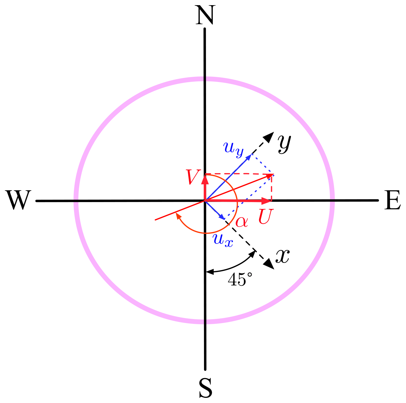
During installing, the coordinates of the sonic anemometer (Campbell CSAT3B), i.e., x, y and z, were in accordance with the observation array, i.e., a 45∘ angle in the northerly direction; see Fig. 3. To retrieve the meteorological wind component from the measured wind velocity components ux, uy and uz, the following equations can be applied,
where u, v and W are the easterly, northerly and vertical components. The wind direction is then calculated as
All parameters obtained are at a sampling frequency of 50 Hz. The measurement resolution is 0.001 m s−1 for ux and uy and 0.0005 m s−1 for uz, respectively. The wind direction can be defined from 0 to 360∘ with an accuracy of at a typical horizontal wind speed of 1 m s−1. Figure 2a–c show the observed meteorological wind speed U, wind direction α and vertical wind velocity W at a height of 3.49 m.
3.2 Air temperature
In addition, the sonic anemometer also provides the air temperature with the same sampling frequency as the wind velocity and a measurement accurate to 0.025 ∘C. Figure 2d shows the collected air temperature with visible outliers, which can be further excluded in analysis using different quality control strategies.
3.3 PM10 concentration
The dust monitor (TSI DustTrak 8530) collected PM10 with a sampling frequency of 1 Hz. The PM10 concentration is on the range of 0.001 to 400 mg m−3 with a typical accuracy of ±0.1 % or . As aforementioned, the measured PM10 concentration is on the range of 0 to 5 mg m−3 with ascending and descending stages that each last for a few hours; see Fig. 2e. Due to a technical reason, the dust sensor at a height of 5 m failed to record the data.
3.4 Quality control
In most instances it is necessary to take many natural factors and events into account, for instance, fierce buoyancy (heat flux) variance and sand and dust movement, to list a few. Quality control methods are necessary to guarantee a good data quality. Generally, the raw data collected from the instrument were necessary to be carried out using pre-processing methods; otherwise, they could be misunderstood as “trustworthy”. Typically, there are generally three types (i.e., missing and unrecognizable characters, extreme values, and values greater than 4 standard deviations) that needed to be pre-processed from the raw data. For the current measurement, there are very few “bad” data; see the temperature curve in Fig. 2d. Therefore, we provide only the raw data with the quality control code.
In general, the following steps can be applied directly to the raw data to remove the outliers. (i) For the “missing” and “unrecognizable characters”: the situations for “data missing” are rare, but the “unrecognizable characters” in the raw data emerge sometimes during a low-battery condition, while the collector (Campbell CR3000) is under a full load or while the GPS is updating. If the irregular point occurs alone, then it was replaced by the mean value on both sides. Otherwise, for some continuous series (less than 1 s, 50 points under the sampling frequency with 50 Hz), they were replaced by the mean values based on the regular points over 1 h. Last, the irregular points greater than 1 s should be considered carefully before using this data series. (ii) Extreme values (for instance, velocity component greater than 100 m s−1 and temperature with 100 ∘C) generally occur as a single point, and it is rare during observation. It is replaced by the mean value on both sides. (iii) For the values greater than 4 standard deviations, the quality control for the database adopts “3σ limits” to produce items of the highest quality, where the data are within 3 standard deviations from the mean to set the upper and lower control limits in statistical quality control charts. Other methodologies are also possible to detect outliers; for instance, instead of 4 standard deviations, one can apply the Hampel identifier to detect the outliers (Davies and Gather, 1993). In this study, to reduce the bias from the interpolation of the data, we replace the outliers by a not-a-number (NaN) variable.
In this section, we present the basic properties of the observed SDS. Without further clarification, the collected data at a height of 3.49 m are presented.
4.1 Nonstationarity
As mentioned above, the SDS event is a typical nonstationary event. Figure 4a shows the hourly averaged curves for both wind speed (U) and PM10, and Fig. 4b shows the corresponding root-mean-square values at a height of 3.49 m. Based on these curves, the observed SDS event can be roughly divided into three stages. (i) During the ascending stage between 09:00 (denoted by A) and 10:00 on 28 March 2016 (denoted by B), the wind speed increases quickly while PM10 starts to rise. (ii) During the stabilizing stage between 10:00 and 17:00 (denoted by C), one sees the strongest wind, which lasts for approximately 7 h. The corresponding PM10 accumulates quickly and reaches its peak value (e.g., ) and maintains it for roughly 3.5 h. (iii) Finally comes the descending stage between 17:00 and 19:00 (denoted by D), where both the wind speed and PM10 are descending sharply. The root-mean-square curves display a similar pattern. Note that a nonlinear trend is evident; see Fig. 4a. When calculating the root-mean-square value, a constant value is subtracted from the raw dataset within a 1 h sliding window, and the trend can not be fully excluded (Wu et al., 2007).

Figure 4(a) Hourly averaged wind speed and at a height of 3.49 m. (b) The corresponding root-mean-square value. This SDS event is roughly divided into three stages, which are illustrated by A–D; see the main text for more detail.
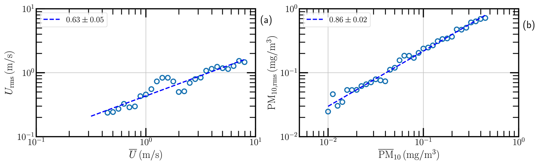
Figure 5(a) Phase diagram of the hourly averaged wind speed versus the root-mean-square speed at a height of 5 m. (b) The hourly averaged concentration PM10 versus its root-mean-square value. The circle is the bin average value with 10 bins for each decade in the logarithmic scale.
Another possible explanation of the above-observed pattern is the amplitude modulation due to the existence of the aforementioned VLSM that is observed in the TABL with typical spatial scales from 𝒪(102 m) to 𝒪(103 m) (Wang and Zheng, 2016) or typical temporal scales from 𝒪(1 min) to 𝒪(10 min) (Wang et al., 2017). The small structures, thus the root-mean-square value, are then modulated by the VLSM (Marusic et al., 2010). This feature is further illustrated as a diagram (hourly averaged value versus the root-mean-square ones) in Fig. 5. The power-law trend is observed with the scaling exponent of 0.63 and 0.86 for the wind speed and PM10, respectively.
4.2 Vertical structure
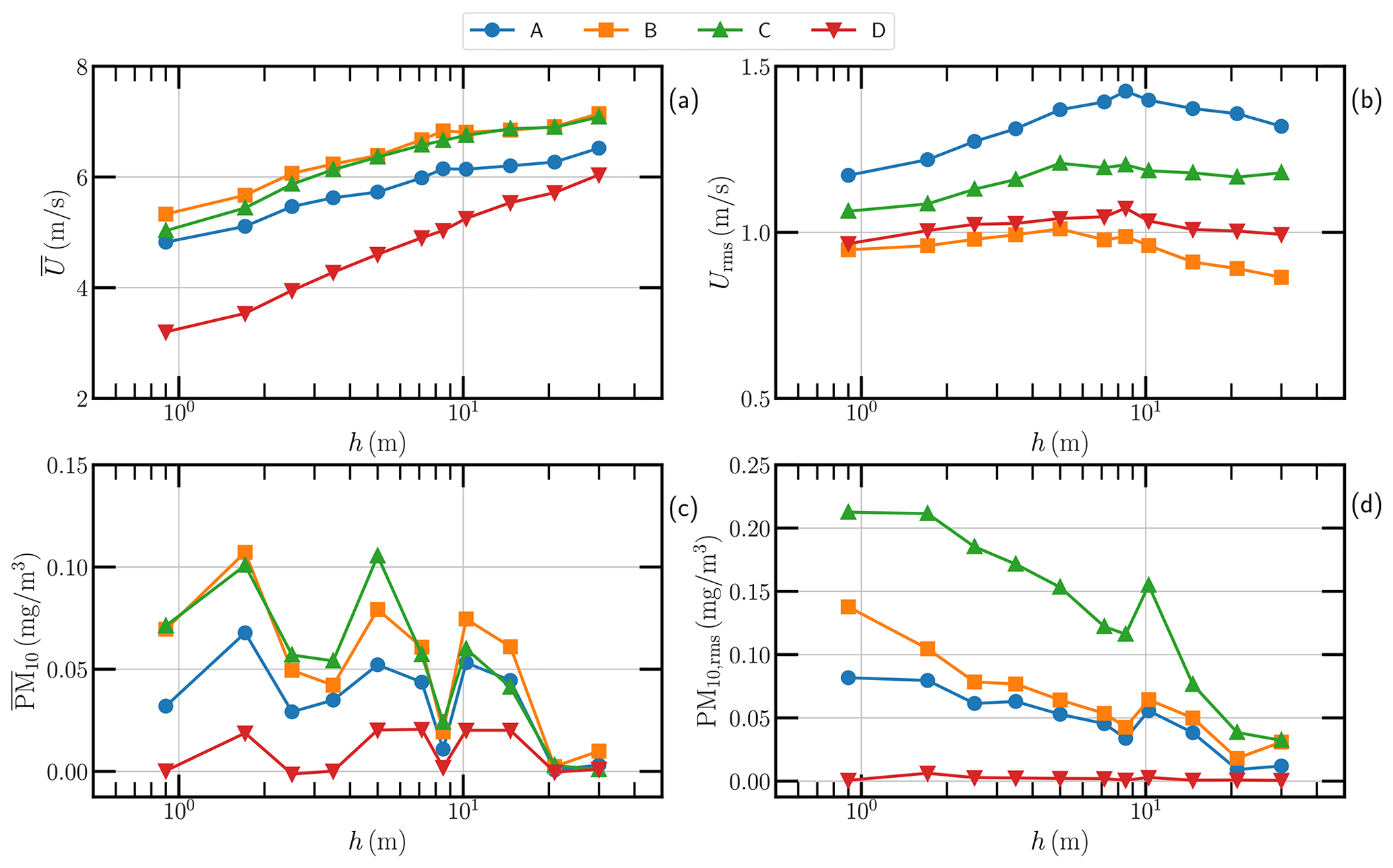
The QLOA is in the logarithmic layer of the TABL, in which the wind speed should vary logarithmically with height that often goes up to 𝒪(102 m) and even to 𝒪(103 m) (Stull, 1997). Figure 6a shows the hourly averaged speed versus h in a semi-log view to emphasize the log law at four time periods from A to D. It suggests that no matter the intensity of the wind speed, the log law of the wall is preserved, which is deeply associated with the TABL. However, the corresponding Urms shows a complex h dependence. It first increases logarithmically with h and reaches its peak, e.g., h=8 m at A, then decreases roughly logarithmically with h. There is no clear h dependence when h≤20 m for the collected in Fig. 6c, while the corresponding PM10,rms clearly logarithmically decreases against h when h<10 m. This is partially due to the interaction between the suspended particles with the turbulent structures, which for sure deserves further investigation.
4.3 Temporal spectral structure
In this work, the Fourier power spectra E(f) are estimated via the Wiener–Khinchin theorem without involving the classical Taylor frozen hypothesis to convert the time measurement to a spatial one (Frisch, 1995). More precisely, the Fourier transform of the autocorrelation ρ(τ) functions as follows:
in which ℛ means the real part; is the complex unit; and
where is the centered θ(xi), θ is the value of either wind speed U or PM10, M(τ) is the sample size at the time separation scale τ, and 〈⋅〉 means average time. With this approach, the estimated Fourier spectrum can recover the correct power-law behavior for the time series with the missing data or irregular time steps without the bias from the interpolation of the data (Gao et al., 2021).
Figure 7a shows the 1 h segment of the raw wind speed U around the typical time periods from A to D at a height of 3.49 m. Fourier power spectra E(f) are then estimated using the abovementioned Fourier spectrum estimator; see Fig. 7b. Due to the existence of atmospheric turbulence, the power-law behavior, i.e., , is observed on the frequency range of Hz with a scaling exponent around 1.53, which is slightly below the classical Kolmogorov value of for three-dimensional homogeneous and isotropic turbulence (Frisch, 1995). This is partially due to the influence of the ground that the scaling exponent βU demonstrates as height dependence. It seems that, except for the intensity of the wind speed, this small-scale scaling feature remains unchanged during the SDS; see Fig. 8.
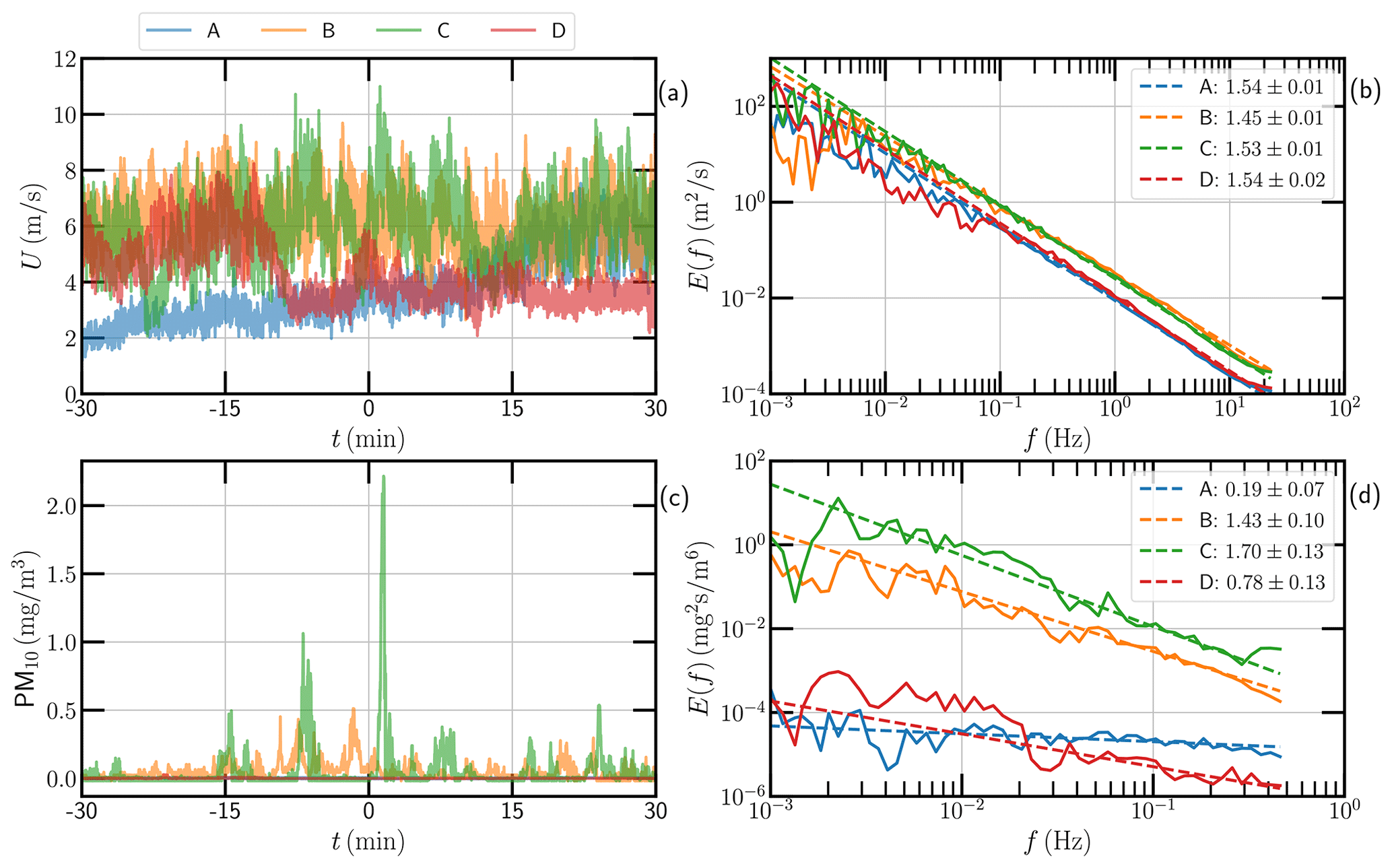
Figure 7(a) Segment of 1 h of the raw wind speed around time A, B, C and D at a height of 3.49 m. (b) The corresponding Fourier power spectrum. (c, d) The PM10 and their Fourier spectra at the same height and time period. The dashed line is the power-law fit for reference.
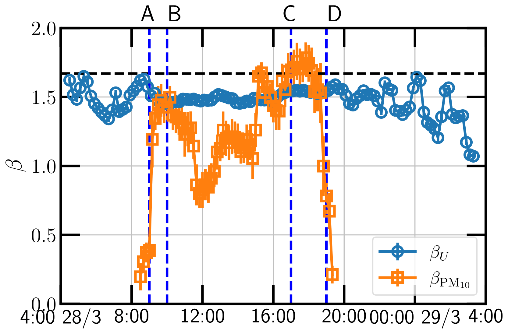
Figure 8Temporal evolution of the scaling exponent β, which is estimated on a 1 h sliding window with 80 % overlap. The horizontal dashed line indicates the Kolmogorov value of for reference. The vertical dash line in Fig. 4 indicates three different stages.
Concerning the concentration of PM10, the scaling feature is more complex; see Fig. 7d and also Fig. 8 for the temporal evolution of the scaling exponents . Note that the density ratio of the sand particle and air is around (Kok et al., 2012). Therefore, the weak wind can not blow the sand particles into the air. The scaling exponents are then approaching zero before the ascending and after the descending periods. During the stabilizing stage, the collected PM10 shows a very intermittent pattern, which can be further linked with the burst events in the TABL; see Fig. 7c. It is interesting to see that the power-law behavior is still preserved and is even closer to the Kolmogorov value; see Fig. 8 for the measured scaling exponent β versus time.
The QLOA site is a one-of-a-kind field observation station that can monitor three-dimensional TABL flows (streamwise, spanwise and wall-normal directions) for both wind-blown sand movement and clean wind, as well as the electric field near the ground surface. The facility's unique measuring array allows us to investigate the three-dimensional shape of coherent structures, as well as the temperature fluctuations that accompany them, which are also covered in this paper. Precious works where the data were collected at the current site can be categorized by three series. (i) The canonical atmospheric turbulent boundary layer is the near-neutral atmospheric surface layer that can be viewed as a truly high-Reynolds-number facility (), where δ is the boundary layer thickness, uτ is the skin-friction velocity and ν is the kinematic viscosity). Characteristics of coherent structures were investigated under near-neutral and stratified conditions (e.g., Wang and Zheng, 2016; Liu et al., 2019; Li and Bo, 2019a; Li et al., 2021b). Roughness effects were explored to illustrate the features in the near-surface layer (e.g., Li and Bo, 2019b; Li et al., 2021c). (ii) Sand-laden flows are wind-blown sand movements that are topically two-phase flows in arid and semiarid regions, where the interaction between flow features and PM10 concentration were previously discussed (e.g., Wang et al., 2017, 2020). (iii) The electric field during an SDS shows granular materials that are regularly brought into contact or collision with one other during dust events such as blowing sand, dust devils and dust storms, generating huge quantities of electrical charge on their surfaces. Measurements of electrical effects in dust events (especially dust storms) have been made specifically and have been further analyzed (e.g., Zhang and Zhou, 2020a, b). Notably, Wang et al. (2020) explored the comparison of large-scale structures of turbulent flows in the atmospheric surface layer with and without sand. According to the research, the streamwise turbulent kinetic energy is enhanced at all scales in the sand-laden flows, and the inclination angles of large-scale structures are shown to increase with sand concentration, owing to the decreased velocity gradient. However, the streamwise length scale of large-scale structures and the size of the most energetic turbulent structures are found to be unaltered compared to clean-air flows. The abundant mechanisms during SDSs are still unknown, especially the difference between the variables during SDS days and those during normal days, which is necessary to be explored in detail in the future.
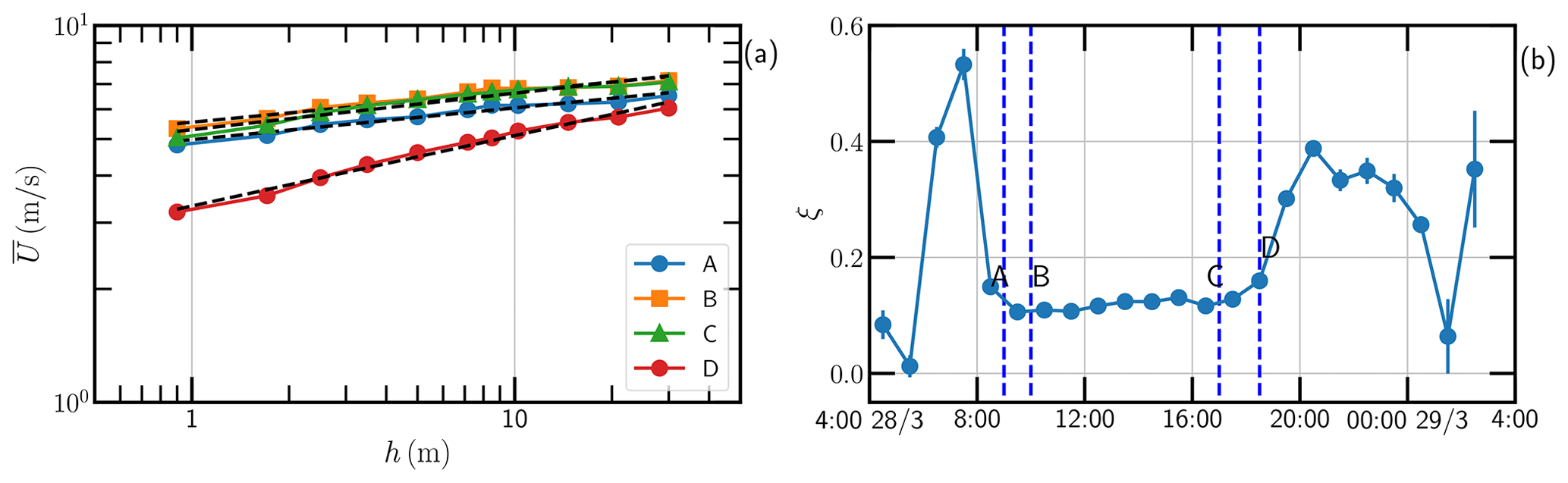
Figure 9(a) Examination of the power-law relation, i.e., , at four typical periods from A to D. The dashed line is a power-law fitting for reference. (b) Temporal evolution of the power-law scaling exponent ξ.
Dust aerosols, being one of the most important types of atmospheric-aerosol constituents, have gotten a lot of attention because of their effects on the environment, weather and climate via radiation and precipitation (Sokolik et al., 2001; DeMott et al., 2003; Zhou et al., 2021). The high-resolution data collected in the current work can benefit researchers who are improving the current sand and dust storm model, as well as the interaction between coherent structures in the flow field and dust field.
5.1 Nonstationarity of the SDS
In general, the TABL shows both daily and seasonal variations due to the rotation and evolution of the earth. Therefore, not only the height of the TABL but also its scaling feature, e.g., scaling of the wind speed and air temperature, show daily and seasonal variations. Within a day, the wind speed, air temperature, etc. often show an intraday trend; see Fig. 4. As aforementioned, it is thus a typical nonstationary event. There exist more rigorous approaches to characterize or analyze the nonstationary time series. For example, a stationary parameter can be defined as quantitatively characterizing nonstationarity (Foken et al., 2004; McCullough and Kareem, 2012). One can also apply either wavelet-based techniques (e.g., wavelet leader and synchrosqueezed wavelet transforms; Flandrin, 1998; Lashermes et al., 2005; Daubechies et al., 2011) or the Hilbert–Huang transform (Huang et al., 1998, 2008; Wu et al., 2007) to extract the local time-frequency information.
It is worth pointing out that the detrending methods should be applied with caution, since the trend is difficult to define and is difficult to separate too (Wu et al., 2007). For example, when calculating the momentum transport (also known as the Reynolds stress) in a wavy aquatic environment, different approaches may provide notable different values (Bian et al., 2018). Therefore, the data-driven approaches, such as wavelet-based techniques or the Hilbert–Huang transform, that can adaptively separate the variations into different scales are recommended to deal with nonstationary SDS data.
5.2 Log law or power law of wind speed
As mentioned above, wind speed is often shown to be logarithmically increasing against height h up to a few hundred meters above the ground; this has been verified at the current site (Wang and Zheng, 2016; Liu et al., 2017). The main assumption of the log law is that the turbulence intensity is only controlled by the amplitude of shear flow and the bottom roughness, relying on the boundary condition. If we consider the situation in the atmosphere, it could be much more complex. Indeed, the convection induced by solar heating brings another source of turbulence that may affect the velocity profile close to the surface, including the influence of sand and dust storms. Meanwhile, the power law is used when surface softness or stability information are not available, even though it has an empirical relation and without a physical basis. There is a simple relationship between the wind speed at one height and that at another; 10 m wind speed is used as the reference level, which is the standard height prescribed by the WMO.
The power-law relation, i.e., , has been proposed (Barenblatt, 1993; Zagarola et al., 1997; Chen and Liu, 2005). The scaling exponent ξ is expected to be constant for an infinite Reynolds number (i.e., , where U is the wind speed; L is the typical length scale, e.g., the height of the sensor location; and ν is the kinetic viscosity of air). It is interesting to note that the power-law relation is evident for the current dataset, since the Reynolds number of the current data is up to 𝒪(107) (Fig. 9). It shows roughly a constant value in the stabilizing stage, since the Reynolds number and wind speed in this period are nearly constant. Note that with such features, a comparison of logarithmic wind profiles and power-law wind profiles is possible.
The dataset was uploaded to a Zenodo repository at https://doi.org/10.5281/zenodo.5034196 (Li et al., 2021a). The datasets are published under the Creative Commons Attribution 4.0 International (CC BY 4.0) license. Additional observation data may be requested from the corresponding author.
High-frequency observatory data for studying the features of the fluid and dust field during sand and dust storms were presented. The complex physical process during the evolution of sand and dust storms is still unknown due to the lack of massive atmospheric observations, especially for high-resolution and synchronous measurements near the surface. For a better understanding of the interplay between turbulent flows and non-turbulent motions during an SDS, a three-stage model was put forward to facilitate the easy understanding of the different fluid and dust features based on the mean velocity changes (also partially taking into consideration the wind direction and PM10 concentration). For the duration of an SDS, structures gradually from ascending to stabilizing to descending effects in turbulent energy and structures were obtained through Fourier spectra, corresponding to the three-stage model. The features revealed in this work grant us a deeper and wider understanding of the SDS fluid and dust field. It is anticipated that data collected in this work will be of utility not only specifically for the boundary layer community in building a model for sand and dust storms but also broadly for communities studying the exchange of the dust and fluid field and energy transfer for the particle-laden two-phase flow.
XZ, GW and XL designed the experiment. XL performed the field observations and data analyses and managed the manuscript with guidance from and editing by YH, GW and XZ. All authors discussed the results and commented on the manuscript.
The contact author has declared that neither they nor their co-authors have any competing interests.
The data are provided as is and with no warranties.
Publisher's note: Copernicus Publications remains neutral with regard to jurisdictional claims in published maps and institutional affiliations.
We thank Haihua Gu, Tianli Bo, Ao Mei, Guowen Han, Yirui Liang, Zhang Huan and Hongyou Liu for their hard work in the field observations. We acknowledge support from the National Natural Science Foundation of China (grant nos. 92052202, 11490553 and 11732010), and Xuebo Li is also supported by a CSC scholarship (file no. 201706180037). Yongxiang Huang is also partially supported by the State Key Laboratory of Ocean Engineering (Shanghai Jiao Tong University) (grant no. 1910).
This research has been supported by the National Natural Science Foundation of China (grant nos. 92052202, 11490553, and 11732010).
This paper was edited by Qingxiang Li and reviewed by two anonymous referees.
Balakumar, B. and Adrian, R.: Large-and very-large-scale motions in channel and boundary-layer flows, Philos. T. R. Soc. A, 365, 665–681, https://doi.org/10.1098/rsta.2006.1940, 2007. a, b
Banta, R. M., Pichugina, Y. L., and Brewer, W. A.: Turbulent velocity-variance profiles in the stable boundary layer generated by a nocturnal low-level jet, J. Atmos. Sci., 63, 2700–2719, https://doi.org/10.1175/jas3776.1, 2006. a
Barenblatt, G. I.: Scaling laws for fully developed turbulent shear flows. Part 1. Basic hypotheses and analysis, J. Fluid Mech., 248, 513–520, https://doi.org/10.1017/S0022112093000874, 1993. a
Bian, C., Liu, Z., Huang, Y., Zhao, L., and Jiang, W.: On Estimating Turbulent Reynolds Stress in Wavy Aquatic Environment, J. Geophys. Res.-Oceans, 123, 3060–3071, https://doi.org/10.1002/2017JC013230, 2018. a
Borbély-Kiss, I., Kiss, A., Koltay, E., Szabo, G., and Bozó, L.: Saharan dust episodes in Hungarian aerosol: elemental signatures and transport trajectories, J. Aerosol Sci., 35, 1205–1224, https://doi.org/10.1016/j.jaerosci.2004.05.001, 2004. a
Chang, Y.-S., Arndt, R. L., and Carmichael, G. R.: Mineral base-cation deposition in Asia, Atmos. Environ., 30, 2417–2427, https://doi.org/10.1016/1352-2310(95)00196-4, 1996. a
Chen, W. F. and Liu, E. M.: Handbook of structural engineering, 2nd Edn., CRC Press, Boca Raton, https://doi.org/10.1201/9781420039931, 2005. a
Daubechies, I., Lu, J., and Wu, H.-T.: Synchrosqueezed wavelet transforms: an empirical mode decomposition-like tool, Appl. Comput. Harmon. A., 30, 243–261, https://doi.org/10.1016/j.acha.2010.08.002, 2011. a
Davies, L. and Gather, U.: The identification of multiple outliers, J. Am. Stat. Assoc., 88, 782–792, https://doi.org/10.2307/2290763, 1993. a
DeMott, P. J., Sassen, K., Poellot, M. R., Baumgardner, D., Rogers, D. C., Brooks, S. D., Prenni, A. J., and Kreidenweis, S. M.: African dust aerosols as atmospheric ice nuclei, Geophys. Res. Lett., 30, 1732, https://doi.org/10.1029/2003GL017410, 2003. a
Flandrin, P.: Time-frequency/time-scale analysis, Academic Press, Cambridge, Massachusetts, 1998. a
Foken, T., Göockede, M., Mauder, M., Mahrt, L., Amiro, B., and Munger, W.: Post-field data quality control, in: Handbook of micrometeorology, Springer, Dordrecht, 181–208, 2004. a
Frisch, U.: Turbulence: the legacy of AN Kolmogorov, Cambridge University Press, Cambridge, England, 1995. a, b
Gao, Y., Arimoto, R., Duce, R., Zhang, X., Zhang, G., An, Z., Chen, L., Zhou, M., and Gu, D.: Temporal and spatial distributions of dust and its deposition to the China Sea, Tellus B, 49, 172–189, https://doi.org/10.3402/tellusb.v49i2.15960, 1997. a
Gao, Y., Schmitt, F. G., Hu, J. Y., and Huang, Y. X.: Scaling Analysis of the China France Oceanography SATellite Along-Track Wind and Wave Data, J. Geophys. Res.-Oceans, 126, e2020JC017119, https://doi.org/10.1029/2020JC017119, 2021. a
Goudie, A. S.: Dust storms: Recent developments, J. Environ. Manage., 90, 89–94, https://doi.org/10.1016/j.jenvman.2008.07.007, 2009. a
Harrison, S. P., Kohfeld, K. E., Roelandt, C., and Claquin, T.: The role of dust in climate changes today, at the last glacial maximum and in the future, Earth Sci. Rev., 54, 43–80, https://doi.org/10.1016/s0012-8252(01)00041-1, 2001. a
Hefflin, B. J., Jalaludin, B., McClure, E., Cobb, N., Johnson, C. A., Jecha, L., and Etzel, R. A.: Surveillance for dust storms and respiratory diseases in Washington State, 1991, Arch. Environ. Health, 49, 170–174, https://doi.org/10.1080/00039896.1994.9940378, 1994. a
Holtslag, A.: Reference module in earth systems and environmental sciences: Encyclopedia of Atmospheric Series, 2nd Edn., Academic Press, Cambridge, Massachusetts, 2015. a
Huang, N. E., Shen, Z., Long, S. R., Wu, M. C., Shih, H. H., Zheng, Q., Yen, N.-C., Tung, C. C., and Liu, H. H.: The empirical mode decomposition and the Hilbert spectrum for nonlinear and non-stationary time series analysis, P. Roy. Soc. Lond. A Mat., 454, 903–995, https://doi.org/10.1098/rspa.1998.0193, 1998. a
Huang, Y., Schmitt, F. G., Lu, Z., and Liu, Y.: An amplitude-frequency study of turbulent scaling intermittency using empirical mode decomposition and Hilbert spectral analysis, Europhys. Lett., 84, 40010, https://doi.org/10.1209/0295-5075/84/40010, 2008. a
Hutchins, N. and Marusic, I.: Evidence of very long meandering features in the logarithmic region of turbulent boundary layers, J. Fluid Mech., 579, 1–28, https://doi.org/10.1017/S0022112006003946, 2007. a, b
Hutchins, N., Chauhan, K., Marusic, I., Monty, J., and Klewicki, J.: Towards reconciling the large-scale structure of turbulent boundary layers in the atmosphere and laboratory, Bound.-Lay. Meteorol., 145, 273–306, https://doi.org/10.1007/s10546-012-9735-4, 2012. a, b
Jickells, T., An, Z., Andersen, K. K., Baker, A., Bergametti, G., Brooks, N., Cao, J., Boyd, P., Duce, R., Hunter, K., Kawahata, H., Kubilay, N., laRoche, J., Liss, P. S., Mahowald, N., Prospero, J. M., Ridgwell, A. J., Tegen, I., and Torres, R.: Global iron connections between desert dust, ocean biogeochemistry, and climate, Science, 308, 67–71, https://doi.org/10.1126/science.1105959, 2005. a
Kok, J. F., Parteli, E. J. R., Michaels, T. I., and Karam, D. B.: The physics of wind-blown sand and dust, Rep. Prog. Phys., 75, 106901, https://doi.org/10.1088/0034-4885/75/10/106901, 2012. a
Kovasznay, L. S., Kibens, V., and Blackwelder, R. F.: Large-scale motion in the intermittent region of a turbulent boundary layer, J. Fluid Mech., 41, 283–325, https://doi.org/10.1017/S0022112070000629, 1970. a
Lashermes, B., Jaffard, S., and Abry, P.: Wavelet leader based multifractal analysis, in: ICASSP 2005 Conference, Philadelphia, USA, https://doi.org/10.1109/ICASSP.2005.1415970, 3–23 March 2005. a
Laurent, B., Marticorena, B., Bergametti, G., and Mei, F.: Modeling mineral dust emissions from Chinese and Mongolian deserts, Global Planet. Change, 52, 121–141, https://doi.org/10.1016/j.gloplacha.2006.02.012, 2006. a
Leys, J. F., Heidenreich, S. K., Strong, C. L., McTainsh, G. H., and Quigley, S.: PM10 concentrations and mass transport during “Red Dawn”– Sydney 23 September 2009, Aeolian Res., 3, 327–342, https://doi.org/10.1016/j.aeolia.2011.06.003, 2011. a
Li, X. and Bo, T.: An application of quadrant and octant analysis to the atmospheric surface layer, J. Wind Eng. Ind. Aerod., 189, 1–10, https://doi.org/10.1016/j.jweia.2019.03.013, 2019a. a
Li, X. and Bo, T.: Statistics and spectra of turbulence under different roughness in the near-neutral atmospheric surface layer, Earth Surf. Proc. Land., 44, 1460–1470, https://doi.org/10.1002/esp.4588, 2019b. a
Li, X., Huang, Y., Wang, G., and Zheng, X.: High frequency observation during the sand and dust storms in the Qingtu Lake Observatory, Zenodo [data set], https://doi.org/10.5281/zenodo.5034196, 2021a. a, b, c, d
Li, X., Wang, G., and Zheng, X.: Study of coherent structures and heat flux transportation under different stratification stability conditions in the atmospheric surface layer, Phys. Fluids, 33, 065113, https://doi.org/10.1063/5.0054205, 2021b. a
Li, X., Wang, G., and Zheng, X.: Turbulent/Synoptic Separation and Coherent Structures in the Atmospheric Surface Layer for a Range of Surface Roughness, Bound.-Lay. Meteorol., https://doi.org/10.1007/s10546-021-00643-z, online first, 2021c. a
Liu, H., Bo, T., and Liang, Y.: The variation of large-scale structure inclination angles in high Reynolds number atmospheric surface layers, Phys. Fluids, 29, 035104, https://doi.org/10.1063/1.4978803, 2017. a
Liu, H., Wang, G., and Zheng, X.: Three-dimensional representation of large-scale structures based on observations in atmospheric surface layers, J. Geophys. Res.-Atmos., 124, 10753–10771, https://doi.org/10.1029/2019JD030733, 2019. a
Marusic, I., Mathis, R., and Hutchins, N.: Predictive model for wall-bounded turbulent flow, Science, 329, 193, https://doi.org/10.1126/science.1188765, 2010. a
McCullough, M. and Kareem, A.: Testing stationarity with wavelet-based surrogates, J. Eng. Mech., 139, 200–209, https://doi.org/10.1061/(ASCE)EM.1943-7889.0000484, 2012. a
McTainsh, G. and Pitblado, J.: Dust storms and related phenomena measured from meteorological records in Australia, Earth Surf. Proc. Land., 12, 415–424, https://doi.org/10.1002/esp.3290120407, 1987. a
Monin, A. S.: The atmospheric boundary layer, Annu. Rev. Fluid Mech., 2, 225–250, https://doi.org/10.1146/annurev.fl.02.010170.001301, 1970. a
Panofsky, H. A.: The atmospheric boundary layer below 150 meters, Annu. Rev. Fluid Mech., 6, 147–177, https://doi.org/10.1146/annurev.fl.06.010174.001051, 1974. a
Shao, Y. and Dong, C.: A review on East Asian dust storm climate, modelling and monitoring, Global Planet. Change, 52, 1–22, https://doi.org/10.1016/j.gloplacha.2006.02.011, 2006. a
Shi, Y., Shen, Y., Kang, E., Li, D., Ding, Y., Zhang, G., and Hu, R.: Recent and future climate change in northwest China, Climatic Change, 80, 379–393, https://doi.org/10.1007/s10584-006-9121-7, 2007. a
Smits, A., McKeon, B., and Marusic, I.: High-Reynolds number wall turbulence, Annu. Rev. Fluid Mech., 43, 353–375, https://doi.org/10.1146/annurev-fluid-122109-160753, 2011. a, b
Sokolik, I. N., Winker, D., Bergametti, G., Gillette, D., Carmichael, G., Kaufman, Y., Gomes, L., Schuetz, L., and Penner, J.: Introduction to special section: Outstanding problems in quantifying the radiative impacts of mineral dust, J. Geophys. Res.-Atmos., 106, 18015–18027, https://doi.org/10.1029/2000JD900498, 2001. a
Stull, R. B.: An Introduction to Boundary Layer Meteorology, Kluwer Academic Publishers, Berlin/Heidelberg, Germany, 1997. a
Sun, J., Mahrt, L., Nappo, C., and Lenschow, D. H.: Wind and temperature oscillations generated by wave–turbulence interactions in the stably stratified boundary layer, J. Atmos. Sci., 72, 1484–1503, https://doi.org/10.1175/jas-d-14-0129.1, 2015. a
Terada, H., Ueda, H., and Wang, Z.: Trend of acid rain and neutralization by yellow sand in east Asia – a numerical study, Atmos. Environ., 36, 503–509, https://doi.org/10.1016/s1352-2310(01)00509-x, 2002. a
Terradellas, E., Soler, M., Ferreres, E., and Bravo, M.: Analysis of oscillations in the stable atmospheric boundary layer using wavelet methods, Bound.-Lay. Meteorol., 114, 489–518, https://doi.org/10.1007/s10546-004-1293-y, 2005. a
Uematsu, M., Duce, R. A., Prospero, J. M., Chen, L., Merrill, J. T., and McDonald, R. L.: Transport of mineral aerosol from Asia over the North Pacific Ocean, J. Geophys. Res.-Oceans, 88, 5343–5352, https://doi.org/10.1029/JC088iC09p05343, 1983. a
UNESCAPReport: Sand and Dust Storms in Asia and the Pacific: Opportunities for Regional Cooperation and Action, Tech. rep., United Nations ESCAP, Bangkok, 2018. a
Wang, G. and Zheng, X.: Very large scale motions in the atmospheric surface layer: a field investigation, J. Fluid Mech., 802, 464–489, https://doi.org/10.1017/jfm.2016.439, 2016. a, b, c, d, e, f
Wang, G., Zheng, X., and Tao, J.: Very large scale motions and PM10 concentration in a high-Re boundary layer, Phys. Fluids, 29, 061701, https://doi.org/10.1063/1.4990087, 2017. a, b, c
Wang, G., Gu, H., and Zheng, X.: Large scale structures of turbulent flows in the atmospheric surface layer with and without sand, Phys. Fluids, 32, 106604, https://doi.org/10.1063/5.0023126, 2020. a, b
Wang, Q., Dong, X., Fu, J. S., Xu, J., Deng, C., Jiang, Y., Fu, Q., Lin, Y., Huang, K., and Zhuang, G.: Environmentally dependent dust chemistry of a super Asian dust storm in March 2010: observation and simulation, Atmos. Chem. Phys., 18, 3505–3521, https://doi.org/10.5194/acp-18-3505-2018, 2018. a
Wu, Z., Huang, N. E., Long, S. R., and Peng, C.-K.: On the trend, detrending, and variability of nonlinear and nonstationary time series, P. Natl. Acad. Sci. USA, 104, 14889–14894, https://doi.org/10.1073/pnas.0701020104, 2007. a, b, c
Yin, S., Anpu, W., Shulan, Y., and Pingsheng, L.: Correlation of acid rain with the distributions of acid and alkaline elements in aerosols, Nucl. Instrum. Meth. B, 109, 551–554, https://doi.org/10.1016/0168-583X(95)00967-1, 1996. a
Zagarola, M. V., Perry, A. E., and Smits, A. J.: Log laws or power laws: The scaling in the overlap region, Phys. Fluids, 9, 2094–2100, https://doi.org/10.1063/1.869328, 1997. a
Zhang, H. and Zheng, X.: Quantifying the large-scale electrification equilibrium effects in dust storms using field observations at Qingtu Lake Observatory, Atmos. Chem. Phys., 18, 17087–17097, https://doi.org/10.5194/acp-18-17087-2018, 2018. a
Zhang, H. and Zhou, Y.-H.: Effects of 3D electric field on saltation during dust storms: an observational and numerical study, Atmos. Chem. Phys., 20, 14801–14820, https://doi.org/10.5194/acp-20-14801-2020, 2020a. a
Zhang, H. and Zhou, Y.-H.: Reconstructing the electrical structure of dust storms from locally observed electric field data, Nat. Commun., 11, 1–12, https://doi.org/10.1038/s41467-020-18759-0, 2020b. a
Zhou, C., Zhang, X., Zhang, J., and Zhang, X.: Representations of dynamics size distributions of mineral dust over East Asia by a regional sand and dust storm model, Atmos. Res., 250, 105403, https://doi.org/10.1016/j.atmosres.2020.105403, 2021. a
Zhuang, G., Yi, Z., Duce, R. A., and Brown, P. R.: Link between iron and sulphur cycles suggested by detection of Fe (n) in remote marine aerosols, Nature, 355, 537, https://doi.org/10.1038/355537a0, 1992. a
Zoljoodi, M., Didevarasl, A., and Saadatabadi, A. R.: Dust events in the western parts of Iran and the relationship with drought expansion over the dust-source areas in Iraq and Syria, Atmospheric and Climate Sciences, 3, 321, https://doi.org/10.4236/acs.2013.33034, 2013. a