the Creative Commons Attribution 4.0 License.
the Creative Commons Attribution 4.0 License.
 | 30 Nov 2021
Arctic sea surface height maps from multi-altimeter combination
Jean-Christophe Poisson
Yannice Faugère
Amandine Guillot
Gérald Dibarboure
We present a new Arctic sea level anomaly dataset based on the combination of three altimeter missions using an optimal interpolation scheme. Measurements from SARAL/AltiKa, CryoSat-2 and Sentinel-3A are blended together, providing an unprecedented resolution for this type of product. Such high-resolution products are necessary to tackle some contemporaneous science questions in the basin. We use the adaptive retracker to process both open ocean and lead echoes on SARAL/AltiKa, thus removing the need to estimate a bias between open ocean and ice-covered areas. The usual processing approach, involving an empirical retracking algorithm on specular echoes, is applied on CryoSat-2 and Sentinel-3A synthetic aperture radar (SAR) mode echoes. SARAL/AltiKa also provides the baseline for the cross-calibration of CryoSat-2 and Sentinel-3A data. The final gridded fields cover all latitudes north of 50∘ N, on a 25 km EASE2 grid, with one grid every 3 d over 3 years from July 2016 to April 2019. When compared to tide gauge measurements available in the Arctic Ocean, the combined product exhibits a much better performance than mono-mission datasets with a mean correlation of 0.78 and a mean root-mean-square deviation (RMSd) of 5 cm. The effective temporal resolution of the combined product is 3 times better than a single mission analysis. This dataset can be downloaded from https://doi.org/10.24400/527896/a01-2020.001 (Prandi, 2020).
- Article
(6078 KB) - Full-text XML
- BibTeX
- EndNote


All components of the Arctic are undergoing large climate changes (Meredith et al., 2019). Among them the Arctic sea ice is certainly the most striking, with dramatic extent (Stroeve and Notz, 2018), thickness and volume losses (e.g., Kwok, 2018). Physical characteristics of the Arctic Ocean are also changing. Ocean temperature is increasing both in the mixed layer (Timmermans et al., 2017) and at depth (e.g., Polyakov et al., 2017). Regarding salinity, the Beaufort Gyre region is freshening (Proshutinsky et al., 2015), while freshwater content decline is reported in other parts of the basin (Armitage et al., 2016). Changes in the Arctic Ocean circulation are also documented, with a strengthening of surface geostrophic currents (Armitage et al., 2017) or intensification of eddy activity (Zhao et al., 2016) in some parts of the basin.
Despite those pressing matters and due to harsh conditions the Arctic Ocean remains poorly observed (Smith et al., 2019). In this context remote sensing, and satellite altimetry in particular, is of great interest. While satellite altimetry was designed to measure the global ocean circulation (Stammer and Cazenave, 2018), it is also used in the Arctic Ocean to retrieve sea level (SL) and sea ice freeboard (Quartly et al., 2019). First estimates of Arctic SL variability from satellite altimetry were made by Peacock and Laxon (2004). The same methodology was successfully used by Giles et al. (2012) to estimate freshwater variations in the Beaufort Gyre. More recently a state-of-the-art Arctic SL dataset (Armitage et al., 2016) has been used to estimate the shape and extent of the Beaufort Gyre (Regan et al., 2019).
Current state-of-the-art Arctic SL datasets (Armitage et al., 2016; Rose et al., 2019) rely on the measurements of one altimeter at a time to produce SL maps with monthly temporal resolution and spatial resolutions of several hundred kilometers, which is not enough to characterize mesoscale activity (Regan et al., 2020). Armitage et al. (2016) processed Envisat and CryoSat-2 data to produce monthly dynamic ocean topography estimates from 2003 to 2014 on a 0.5∘ latitude by 0.75∘ longitude grid. Rose et al. (2019) processed the full altimeter record from 1991 (ERS-1) to 2019 (CryoSat-2). Monthly sea level anomaly (SLA) fields are available on a 0.25∘ latitude by 0.5∘ longitude grid. The field is interpolated onto the grid using a least squares collocation technique and specifying correlation scales of 500 km. Both those datasets are undefined above 81.5∘ N.
The combination of several altimeters can improve the resolution of global SL maps (Ducet et al., 2000; Pascual et al., 2006). This multi-mission combination is operational in the Data Unification and Altimeter Combination System (DUACS) (Pujol et al., 2016; Taburet et al., 2019). In this paper we present a new Arctic SL dataset based on the combination of three satellite altimetry missions: SARAL/AltiKa (SRL), Sentinel-3A (S3A) and CryoSat-2(C2). Section 2.2 details the along-track data processing scheme, as well as the standards used. The multi-mission cross-calibration and combination methods are described in Sect. 2.3. Results of the data quality assessment are presented in Sect. 4.
SL estimation in the ice-covered Arctic Ocean relies on the identification of radar waveforms originating from leads (cracks) in the ice pack where the ocean surfaces (Quartly et al., 2019). All groups (Armitage et al., 2016; Rose et al., 2019) follow the same general workflow, but processing details can be different. In this section we describe our regional Arctic sea level processing: data sources (Sect. 2.1), echo classification (Sect. 2.2.1) and retracking (Sect. 2.2.2), lead selection (Sect. 2.2.3), geophysical corrections (Sect. 2.2.4), and data editing (Sect. 2.2.5) and mapping (Sect. 2.3).
2.1 Satellite radar altimetry missions
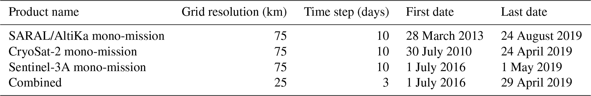
We processed measurements from three satellite altimetry missions: SARAL/AltiKa, Sentinel-3A and CryoSat-2. Some relevant characteristics of these missions are summarized in Table 1. A brief description of each mission is given below.
2.1.1 SARAL/AltiKa
SARAL/AltiKa (herein abbreviated SRL) is a joint French (CNES) and Indian (ISRO) satellite radar altimetry mission (Verron et al., 2015). Its main instrument is a Ka-band pulse-limited radar altimeter. The higher frequency compared to Ku-band missions, combined with a higher pulse repetition frequency permits a higher along-track sampling. A better range resolution is also achieved thanks to a larger bandwidth (Steunou et al., 2015). SRL was launched in February 2013 and is still operational today. Initially launched on the Envisat orbit it provides measurements up to 81.5∘ latitude. SRL data used in this study are taken from the CNES PEACHI project dataset (Valladeau et al., 2015).
2.1.2 CryoSat-2
CryoSat-2 (herein abbreviated C2) was launched in April 2010 and is an ESA satellite radar altimetry mission designed to monitor the Earth's cryosphere (Wingham et al., 2006). Polar regions are observed up to 88∘ thanks to its 92∘ orbit inclination. The SAR Interferometric Radar Altimeter (SIRAL) radar on board CryoSat-2 can operate in low-resolution mode (LRM), synthetic aperture radar (SAR) mode or synthetic aperture interferometric mode (SARIn). The switch from one mode to another is based on a geographical mode mask. SAR mode is generally used over sea ice areas and provides an unprecedented along-track resolution of 300 m. In this study, only SAR mode data from C2 are used, and the area covered therefore varies over time with the geographical mode mask. C2 data used in this study are L1b data taken from ESA payload data ground segment Ice Baseline C processor. The Payload Data Ground Segment (PDGS) Ice processor includes zero padding and Hamming windowing which reduce the impact of antenna side lobes and increase the range resolution over peaky echoes (Smith and Scharroo, 2015).
2.1.3 Sentinel-3A
Sentinel-3A (herein abbreviated S3A) is a Copernicus mission providing sea surface topography measurements (among other variables) thanks to its SRAL (Sentinel-3 Radar ALtimeter) SAR mode altimeter (Donlon et al., 2012). S3A provides measurements up to 81.5∘ latitude. Compared to C2, S3A always operates in SAR mode whether over open ocean or ice-covered areas. S3A was launched in February 2016 with an expected lifetime of 7 years. For S3A no operational ground segments implement zero padding or Hamming windowing (Lawrence et al., 2019). We therefore rely on data from the CNES S3A Processing Prototype (S3PP), an experimental SAR processing chain derived from previous work on CryoSat-2 (Boy et al., 2017) which does include these algorithms.
2.2 Along-track data processing
2.2.1 Waveform classification
Waveform classification aims at separating radar altimetry waveforms based on their shape to identify echoes from leads, floes and open ocean. In Arctic SL studies, classification generally relies on the pulse peakiness (Peacock and Laxon, 2004, for example): peaky echoes are associated with leads which act as bright targets in the radar footprint. New classification methods were more recently introduced such as unsupervised clustering based on several waveform-derived features (Müller et al., 2017). Here we use the neural-network-based classification method proposed by Poisson et al. (2018). This classification method provides a wealth of information with 16 output classes. Classification outputs were validated against coincident SAR images from Sentinel-1 by Longépé et al. (2019), especially for sea ice lead detection. For the purpose of this study we only select echoes labeled as class 1 (Brownian echoes, associated with open ocean) and class 2 (peaky echoes, associated with sea ice leads). For C2, the geographical SAR mode mask varies over time to match sea ice extent, and since we only process C2 SAR mode data, only a very small fraction of the open ocean is observed. These data (Brownian C2 echoes) are discarded from the analysis.
2.2.2 Retracking
Retracking designates the process of extracting geophysical parameters from the radar waveforms. There is a variety of retracking algorithms, from purely empirical algorithms to physical ones which require a waveform model. In this study several retracking algorithms are used depending on the measurement mode (LRM or SAR) and echo type (Brownian or peaky). For SRL, all echoes are retracked by the adaptive algorithm (Poisson et al., 2018). This physical retracker provides a processing continuity between open ocean and ice-covered areas, thus removing the need to estimate a bias between the two surfaces. This represents an important difference with respect to other Arctic SL datasets (Armitage et al., 2016) in which different retracking algorithms are used to process open ocean and leads. C2 and S3A operate in SAR mode, and we fall back to using different retracking algorithms over sea ice and open ocean areas. At this stage sea ice and open ocean selection is based only on the outcome of the waveform classification. On S3A, class 2 (peaky) echoes are retracked by the threshold first maximum retracker algorithm (TFMRA) (50 % threshold; Helm et al., 2014), while class 1 (Brownian) echoes are retracked using the standard ocean (MLE3) algorithm. For C2 only class 2 (peaky) echoes are kept in the analysis, and they are retracked using the TFMRA algorithm (50 % threshold).
2.2.3 Ocean and lead selection
After waveform classification and retracking, a second stage of the ocean and lead selection algorithm is applied. This algorithm is based on three parameters: sea ice concentration (SIC) taken from OSI-450 product (Lavergne et al., 2019), waveform class and radar backscatter coefficient. All class 1 (Brownian) echoes in areas where SIC is lower than 30 % are considered to represent the open ocean. All class 2 echoes with enough backscattered power over areas where SIC is greater than 30 % are considered to be lead echoes. Backscattering distributions differ for each mission, and therefore backscattering thresholds are different for SRL, S3A and C2. Thresholds used in this study are given in Table 2. These thresholds were empirically set based on the comparison of backscatter distributions for class 2 and class 4 and 6 echoes (associated with sea ice floes; Longépé et al., 2019).
Leads act as bright targets in the radar footprint, and their contribution tends to be dominant even when they represent a small fraction of the radar footprint. This can lead to the retracker following off-nadir targets and biasing range estimates. This effect is called “snagging” (Peacock and Laxon, 2004) or “hooking” (Boergens et al., 2016). SRL, as an LRM altimeter, is more prone to this phenomenon than S3A and C2. Here we use the method proposed by Poisson et al. (2018) to remove measurements identified as leads that may be affected by hooking. Hooking removal is based on the selection of the maximum backscatter echo within a moving window.
SAR altimetry is less sensitive to such effects due to the much smaller along-track resolution, and no hooking flag is applied to S3A and C2. Note that this does not account for cross-track hooking errors which were investigated by Armitage and Davidson (2014), resulting in an estimated −1 to −4 cm bias on ocean topography itself and are neglected in the present study.
(Iijima et al., 1999)(Carrère and Lyard, 2003)Desai et al. (2015)(Carrère et al., 2016)(Cartwright and Edden, 1973)(Andersen et al., 2016)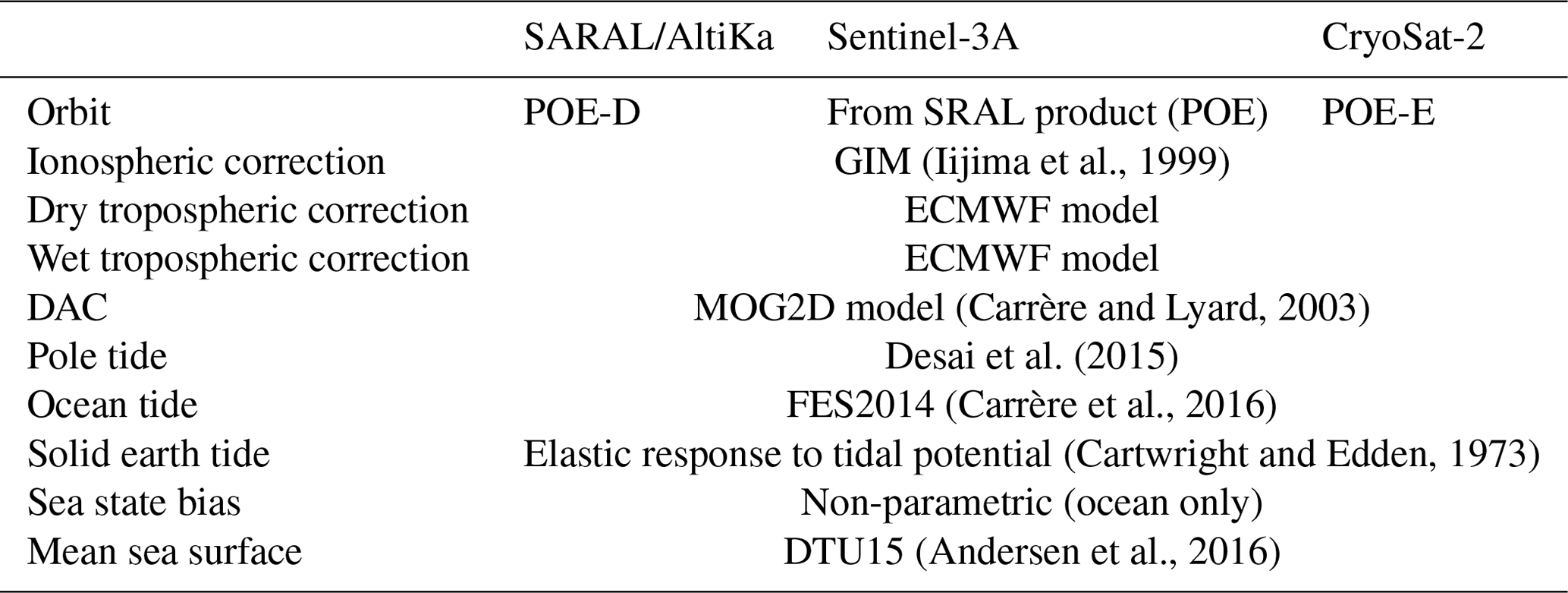
2.2.4 Sea level anomaly estimation
Once relevant radar echoes are selected and retracked to estimate the radar range, one can estimate sea levels. Classically sea level is estimated following Eq. (1) (e.g., Chelton et al., 2001).
where the corrections account for a range of geophysical and instrumental effects, and MSS signifies mean sea surface. The standards and models used in this study are given in Table 3. The corrections used are not uncommon and are mainly derived from DUACS processing (Taburet et al., 2019), with three notable exceptions:
-
We use the DTU15 mean sea surface (Andersen et al., 2016), which thanks to its use of C2 is defined over the whole Arctic domain.
-
Over leads, the sea state bias correction is set to zero, as we consider that over these small open water stretches waves are small.
-
The radiometer wet tropospheric correction is undefined over sea ice, and we therefore use a modeled wet tropospheric correction over the whole product domain.
2.2.5 Data editing
The data editing is a crucial step for final product quality and is always the result of a balance between data quality and coverage. The most fundamental editing is the ocean and lead selection algorithm described above, yet this may retain erroneous measurements. Here we tried to remove obvious outliers while retaining as many measurements as possible to build the final SL product. First we apply a basic thresholding to remove any SL anomalies greater than 2 m (absolute deviation). Over open ocean areas, an iterative editing process is applied. The iterative editing processes along-track segments and removes measurements more than 2.5 standard deviations from the segment mean. For this iterative editing to work continuous segments are required. This requirement is not met over ice-covered areas, and the iterative editing is not applied to lead measurements. Following Rose et al. (2019) we also apply a statistical editing based on local SL anomaly variance levels derived from a coarse gridding (200 km) of each mission's data. Measurements that are locally more than 2.5σ from a 3-month running mean are discarded. This methods takes into account local SL variance levels, and the running mean prevents systematically removing measurements at highs and lows of the seasonal cycle.
2.2.6 Ocean and lead bias correction
S3A data are retracked by different algorithms over open ocean and leads. This introduces a discontinuity that must be corrected empirically (Giles et al., 2012). Armitage et al. (2016) faced a similar issue and proposed a correction method comparing sea ice and open ocean echoes near the sea ice edge. Using a similar methodology leads to an average lead and ocean bias of around 16 cm for S3A with a large uncertainty. Using the adaptive retracker on SRL means that a baseline is available to estimate the lead and ocean bias for S3A. Comparing SRL and S3A over leads and ocean results in a S3A lead and ocean bias estimate of 11 cm. This emphasizes the importance of processing continuity for at least one mission, which can be used as a reference, to ensure final product accuracy. As we only process lead echoes for C2, no lead and ocean bias estimation is required.
2.3 Multi-mission combination
After the operations described in Sect. 2.2 we are left with an ensemble of valid SL anomaly measurements along the track of three different satellite radar altimeters. While this is already enough to estimate mono-mission products (see Sect. 3), our goal here is to combine all three missions together to increase SL map resolution. The methods used here are derived from the DUACS processing (e.g., Le Traon and Dibarboure, 1999; Pascual et al., 2006) with adaptations to fit the Arctic Ocean.
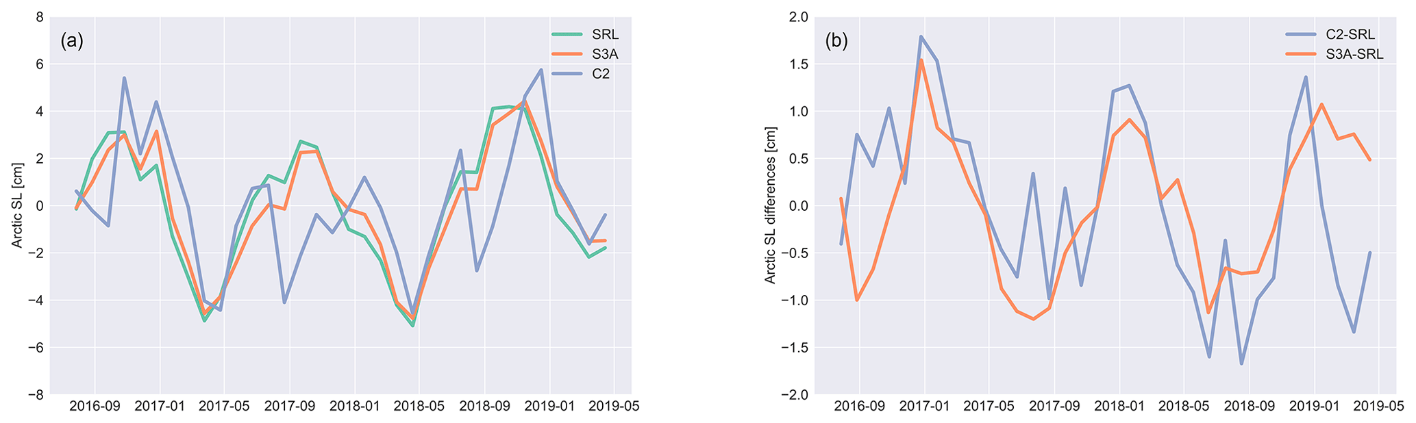
Figure 1Time series of Arctic regional sea level for SRL, S3A and C2 (a), as well as regional sea level differences between C2 and SRL and S3A and SRL (b).
2.3.1 Cross-calibration
Cross-calibration is designed to remove long-wavelength errors (LWEs) in along-track altimetry prior to the optimal interpolation (OI). In a typical global ocean processing inter-mission cross-calibration would be performed through empirical orbit error estimation (Le Traon and Ogor, 1998). Orbit error estimation requires a global crossover dataset which is not available in this case as we processed only areas north of 50∘ N. Moreover empirical orbit errors are not well constrained over the Arctic, which is surrounded by large continental areas where no crossovers are available. As a result a much simpler regional bias removal technique is used here, which is based on the comparison of regional SL estimates from the three altimeters.
Time series of regional SL for SRL, C2 and S3A are shown in Fig. 1. These time series are estimated over the whole domain of each mission using box averages. For SRL and S3A, domains are consistent through time, and both missions observe similar regional SL variability. For C2, only sea ice lead measurements are used; hence larger discrepancies with respect to SRL and S3A are observed in summer months when sea ice extent is small. Differences are estimated over the common domain of two missions (Fig. 1, right panel), and discrepancies between SRL and C2 are reduced. In both cases differences exhibit an annual pattern with an amplitude around 1 cm. The higher month-to-month variability observed in the C2 minus SRL difference with respect to S3A minus SRL is the result of a smaller and more variable geographical cover on the former.
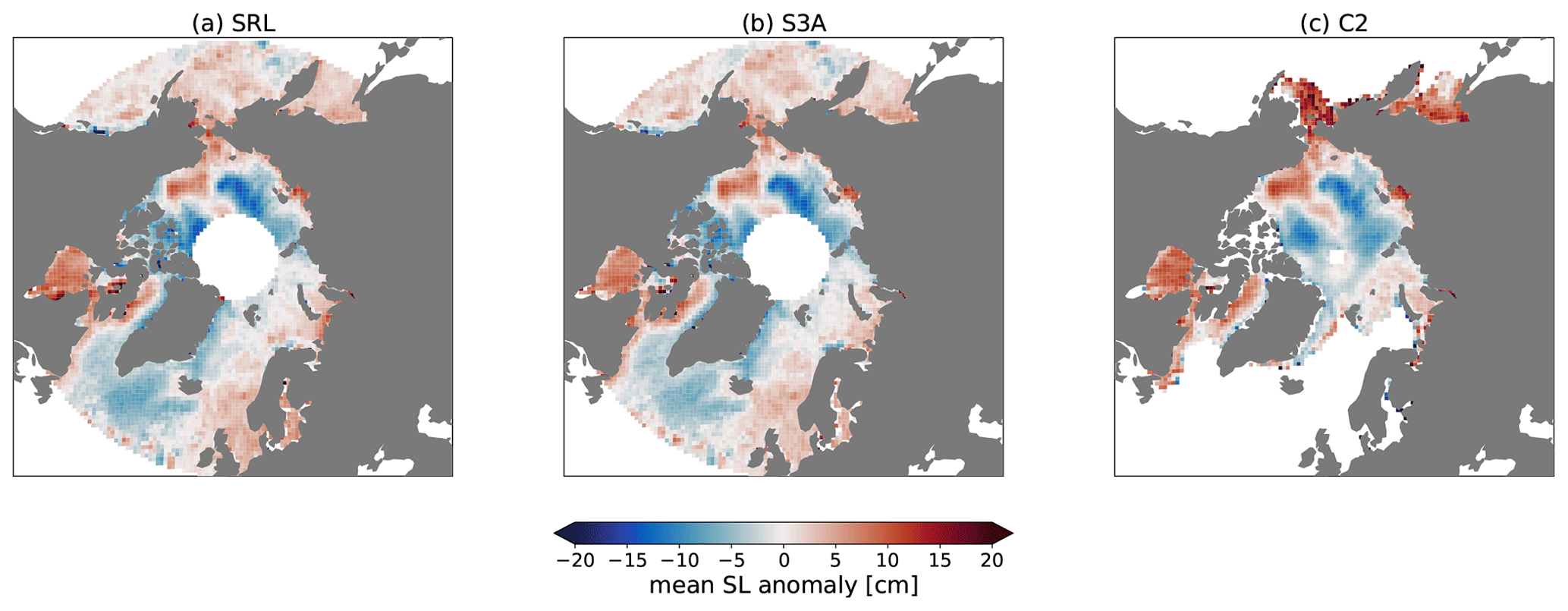
Figure 2Mean Arctic SLA maps for SRL (a), S3A (b) and C2 (c). All maps are estimated over the time span common to all missions (July 2016–April 2019).
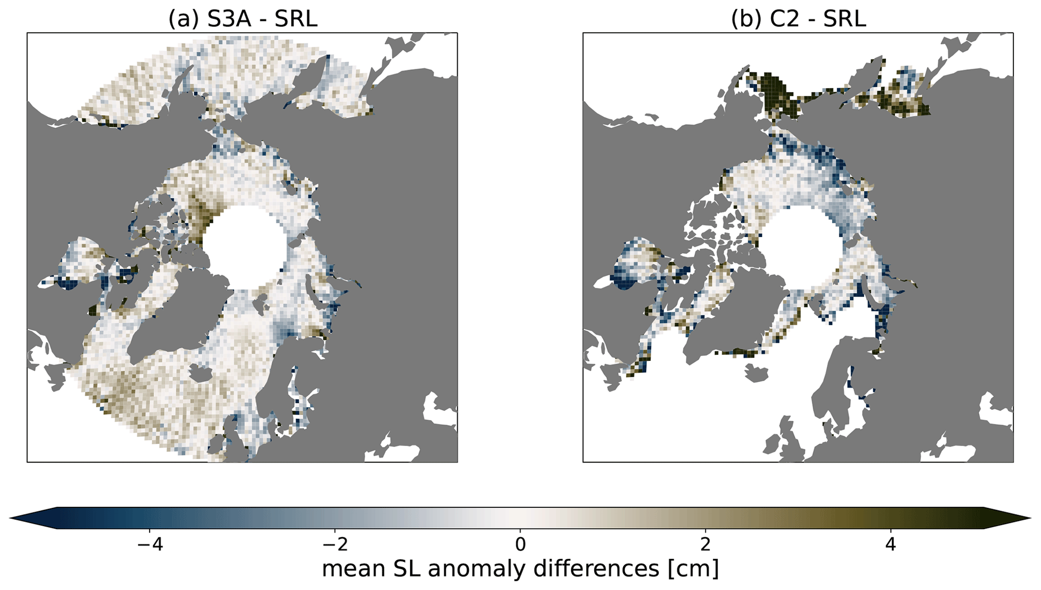
Figure 3Maps of mean SL differences between (a) S3A and SRL and (b) C2 and SRL. Differences are estimated over the time span common to all missions (July 2016–April 2019).
We fit and remove a 1-year period sine wave to correct for the time-dependent part of the intermission bias. Geographically dependent biases were also investigated: maps of average SL are shown in Fig. 2 and maps of SL differences between C2 and SRL and S3A and SRL in Fig. 3. Differences remain small (below 2.5 cm) except along the coasts and at the sea ice edge for C2. Some large-scale geographical patterns are observed: higher SLA values for C2 and S3A than for SRL in the multi-year ice region north of the Canadian Arctic Archipelago are not easily modeled and are left uncorrected.
2.3.2 Along-track filtering and subsampling
Before the optimal interpolation open ocean along-track SL anomaly measurements are filtered and sub-sampled to reach a 5 Hz resolution. Using 5 Hz measurements rather than the full altimeter resolution significantly reduces the processing time for the optimal interpolation with almost no impact on the estimated fields. Measurements over the ice-covered Arctic Ocean are left at the full resolution of the altimeter.
2.3.3 Optimal interpolation
We use an optimal interpolation (OI) scheme to map SL anomaly fields on a regular grid. OI is based on an inverse formulation first introduced in oceanography by Bretherton et al. (1976). The methodology used here is derived from the DUACS global processing (Le Traon and Dibarboure, 1999; Ducet et al., 2000) with some adaptations to the Arctic Ocean which are described below. The quality of interpolated fields depends on the accuracy of several prior fields such as signal variance, covariance scales and error levels.
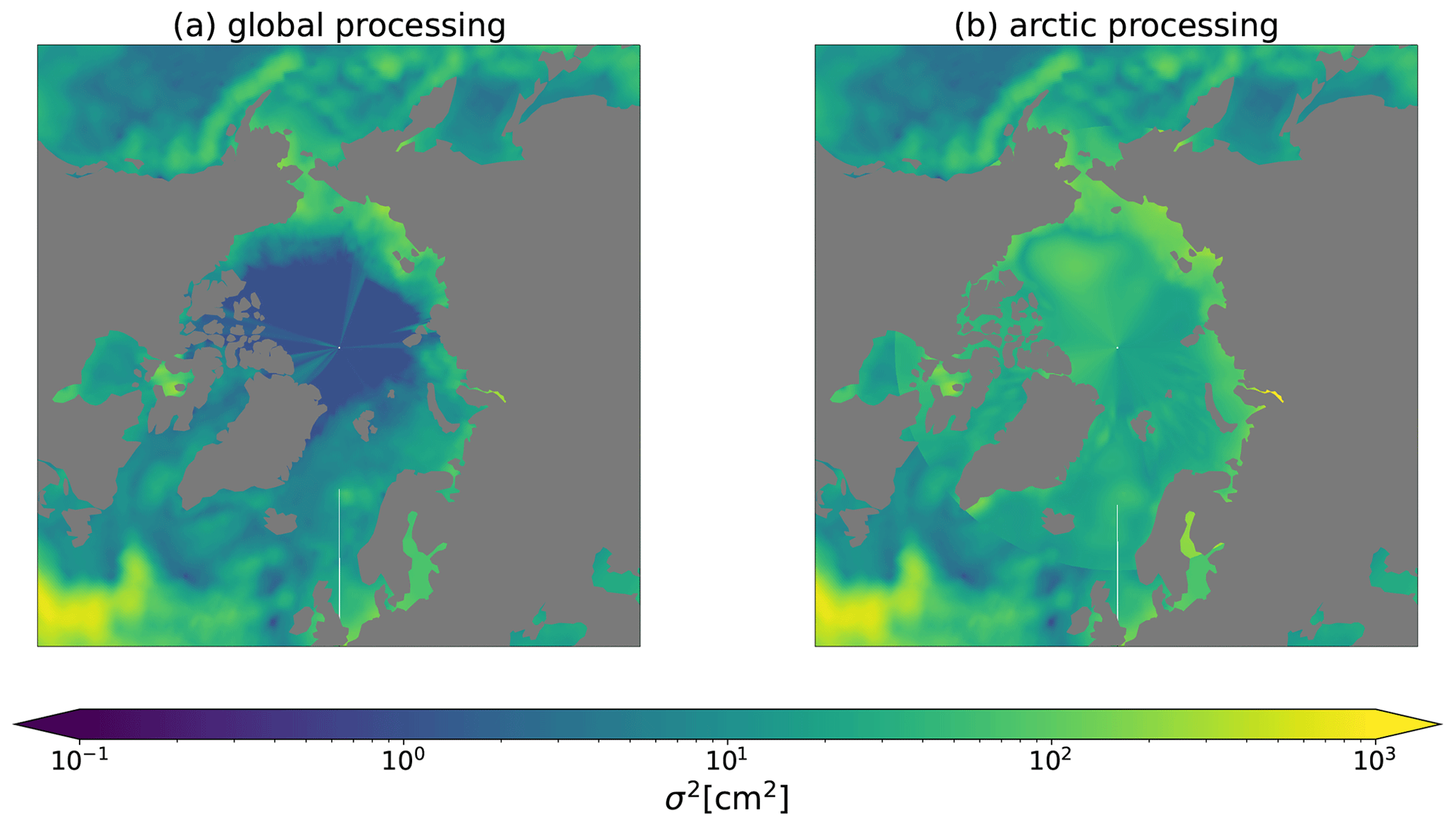
Figure 4A priori signal variance maps used in (a) DUACS global processing and (b) the Arctic regional processing.
Signal variance and error levels were adapted from currently used global values (Taburet et al., 2019) to fit the Arctic. One important adaptation is an updated prior for signal variance. The signal variance map currently used in the DUACS global processing is shown in Fig. 4 (left panel) and shows large drop at latitudes inside the Arctic Ocean. An analysis of the Centre for Polar Observation and Modelling (CPOM) dataset (Armitage et al., 2016) or the Climate Change Initiative (CCI) dataset (Rose et al., 2019) does not show the same pattern. Unrealistically low variance levels will cause the interpolation to dampen signals during the mapping, which is unwanted. We estimate an updated signal variance map by locally taking the maximum variance level among DUACS, CCI and CPOM data for latitudes greater than 60∘ N. The resulting variance map is shown in Fig. 4 (right panel). This method introduces a discontinuity, which shall be addressed in future versions of the product, but does not impact the final product variance (see Fig. 7, right panel).
Two terms control the prior error level in the input data: uncorrelated noise and long-wavelength errors (LWEs). Accurate error priors will prevent error artifacts being interpreted as real signals during the interpolation. Both were tuned to account for regional characteristics. DUACS standard processing uses different noise levels for different missions, reflecting the actual level of noise of each mission, plus the unobservable part of the ocean dynamics. For the Arctic dataset, we rely on a simpler approach with a noise level for open ocean measurements: one for leads measurements and one for LWEs. Uncorrelated noise level priors are derived from existing DUACS noise levels under the following assumptions:
-
Over ocean, our measurements should be slightly noisier than the standard processing due to the modeled wet tropospheric correction and a less accurate mean sea surface model (Pujol et al., 2018).
-
Over sea ice, noise levels should be even higher due to increased errors in geophysical corrections and in range retrieval from peaky waveforms.
-
Noise levels should be scaled to account for the fact that we are using 5 Hz or 20 (40) Hz measurements depending on the surface.
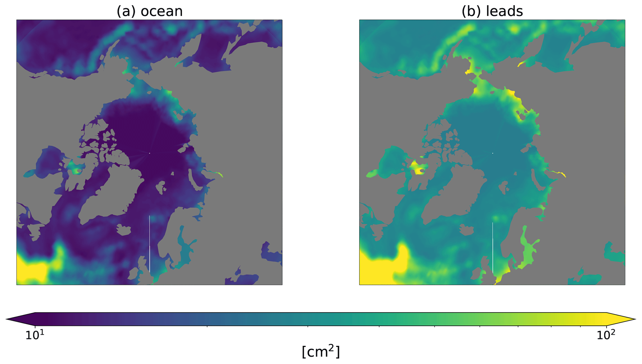
Figure 5Noise levels over open ocean (a) and ice-covered (b) areas used in the regional analysis.
The ice-covered noise level is empirically derived from open ocean noise by adding 5 cm2, based on the analysis of measurement distributions over both surfaces, and accounting for the use of high-resolution measurements. Open and ice-covered ocean uncorrelated noise level priors are shown in Fig. 5.
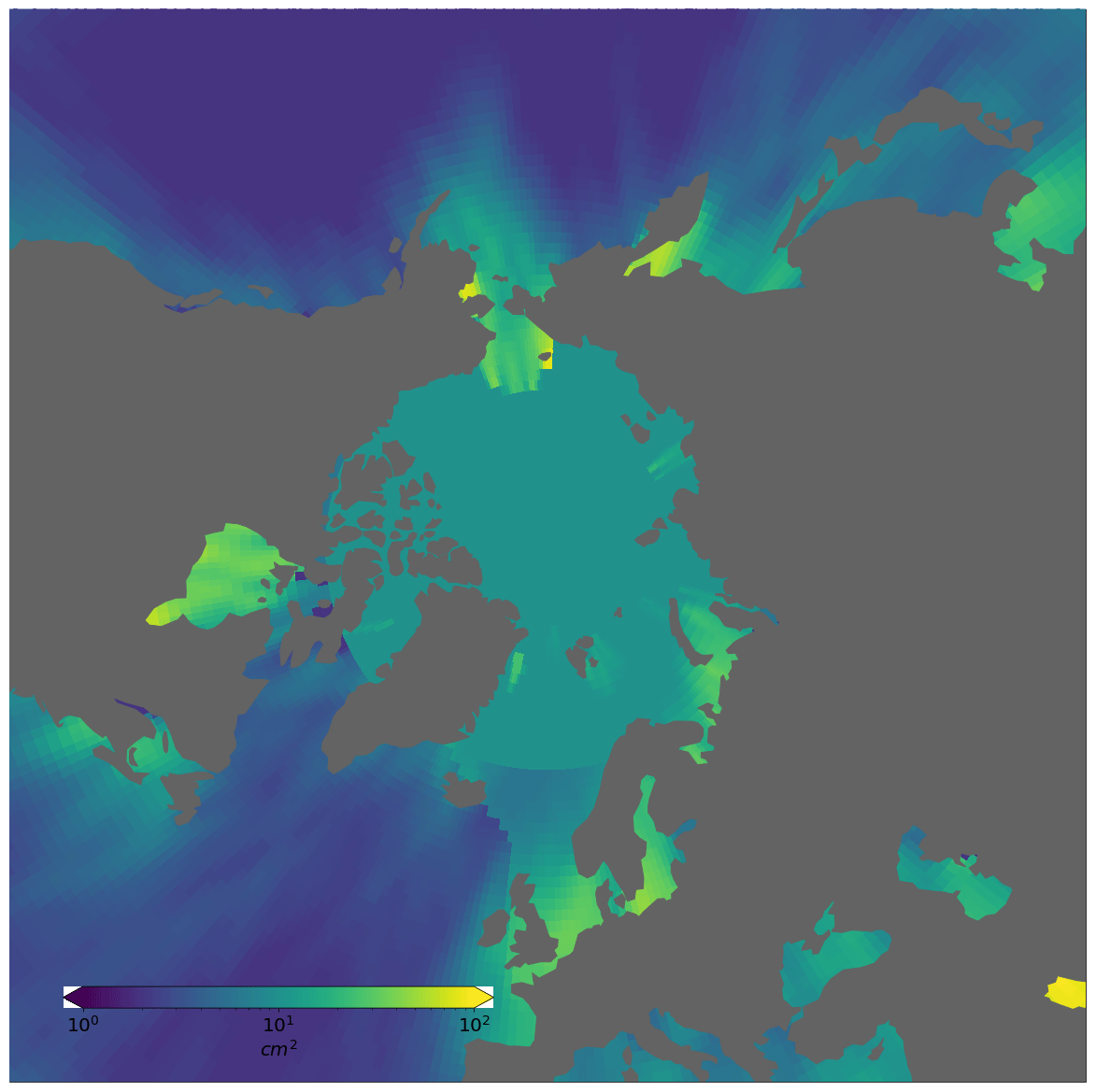
Figure 6Variance of LWEs used for the Arctic Ocean optimal interpolation.
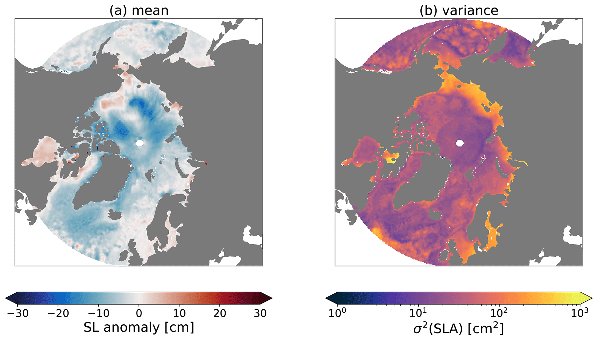
Figure 7Maps of (a) mean SL and (b) variance of SL in the Arctic Ocean from the combined product.
LWEs are designed to absorb correlated errors along-track coming from errors in geophysical models such as the tide and DAC (dynamical atmospheric correction) corrections. For this regional analysis, they should also be able to absorb residual orbit errors, which are not corrected due to the lack of a proper cross-calibration. Again we derive the LWE priors from existing DUACS priors and set a minimum LWE variance of 10 cm2 for all latitudes greater than 68∘ N to account for uncorrected radial orbit errors. This value was empirically set based on the analysis of global empirical orbit error corrections (available from DUACS) which provide a proxy for radial orbit errors. The resulting LWE variance distribution, which is used for all three missions considered here, is shown in Fig. 6. Again, our prior estimation method does introduce some discontinuities that shall be addressed in future dataset version, but these do not appear to have a large negative impact on product quality.
Correlation scales are kept unchanged from the DUACS global processing, and SL anomaly fields are interpolated onto a 25 km EASE2 grid (Brodzik et al., 2012, 2014) every 3 d.
The combined product is distributed as a single NetCDF file containing maps of SL anomalies and absolute dynamic topography (ADT). ADT fields are obtained by adding the DTU15 mean dynamic topography (MDT) (Andersen et al., 2016) to SL anomaly fields.
We also provide three mono-mission products for SRL, C2 and S3A which are available over longer periods (see Table 4) depending on input data availability at product generation time. These are the result of simple box averages of along-track measurements with no cross-calibration. Due to their mono-mission nature, they are only available at a lower resolution (75 km, 1 month).
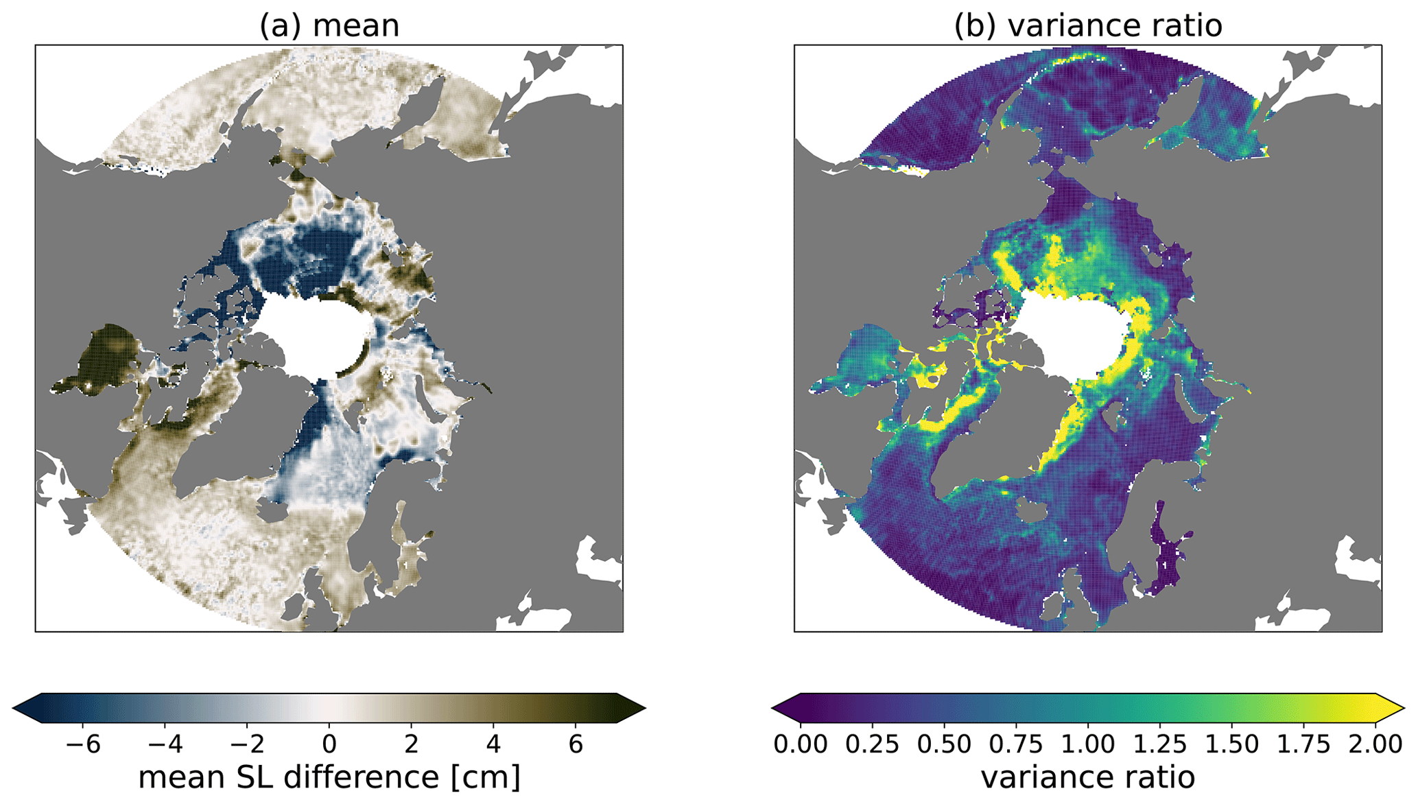
Figure 8Differences between arctic product and CMEMS global products: (a) mean difference and (b) variance of the differences expressed as a fraction of signal variance.
In this section we present some product validation results. Assessing the product accuracy is difficult in the Arctic Ocean as few independent validation datasets are available (Smith et al., 2019). Here we rely on comparisons between mono-mission products (Sect. 4.1), analysis of regional statistics (Sect. 4.2), comparisons to the DUACS global product (Sect. 4.3) and comparisons to tide gauge data available in the basin (Sect. 4.4) .
4.1 Mono-mission product comparisons
Time series of the regional average sea level in the Arctic Ocean from SRL, S3A and C2 are shown in Fig. 1, while maps of the average SL anomalies are shown in Fig. 2. All three missions exhibit very consistent behaviors considering SL variations over time, as well as geographical patterns, even before any type of cross-calibration is applied. This is already a good indication that observed variations are not artifacts arising from errors in the data. Regional average SL differences remain below 2 cm (see Fig. 1, right panel). Differences in geographical patterns (see Fig. 3) are slightly larger with differences (up to 5 cm) found on the coast, near the sea ice edge and to a lesser extent in the thicker ice zones north of Greenland and the Canadian Arctic Archipelago.
4.2 Regional statistics
Maps of the mean SL and variance of SL in the Arctic Ocean, derived from the combined products, are shown in Fig. 7. SL variance levels are consistent throughout the Arctic Basin. This suggests a good product accuracy as high variance levels in the interior of the Arctic Ocean would be an indication of errors. The variance distribution is consistent with previous datasets (Armitage et al., 2016; Rose et al., 2019) with high variance levels along the Russian Arctic coasts. Such variance levels could result from continental shelf wave propagation (Danielson et al., 2020). Another prominent feature is the SL variance's slight drop above 81.5∘ N. This is expected, as in this area C2 is the only radar altimeter mission, and the product is therefore unable to reach the same resolution as at lower latitudes.
Table 5Comparisons to tide gauges. RMSd values are given in meters.
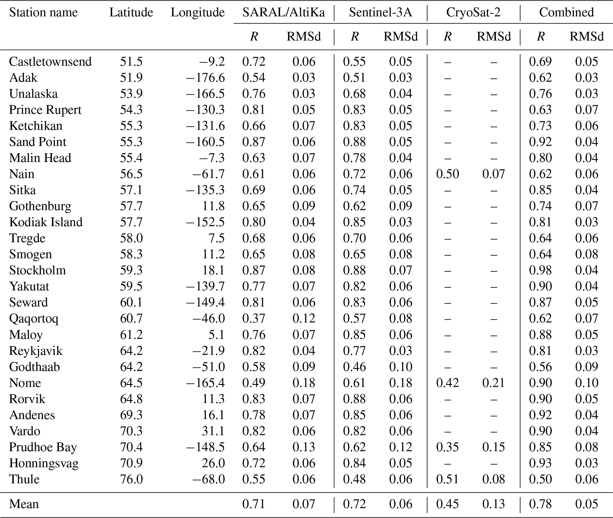
Figure 7 also shows the mean Arctic Ocean SL from the combined products. First, there is no large bias between the open ocean and the seasonally ice-covered areas, suggesting that our lead detection and retracking algorithms perform well. A negative geometric patch is visible north of the Canadian Arctic Archipelago in the so-called “Wingham box” where C2 operated in SARIn mode from April 2011 to July 2014 (geographical mode mask versions 3.2, 3.3 and 3.4). There are no SARIn data over the period considered here, and this bias is certainly coming from the MSS. Another bias is clearly visible between the Labrador Sea and Hudson Bay, and is extends up north into the western parts of Baffin Bay. The origin of this pattern remains to be investigated: it could again be an error in the MSS or an issue in our current classification and retracking methods in this area.
4.3 Comparisons to the DUACS global product
The Arctic regional product presented here focuses on SL estimation in ice-covered areas, and its accuracy over open ocean might be hindered by some processing choices such as using the modeled wet tropospheric correction or the lack of a proper cross-calibration prior to the optimal interpolation. Comparing the Arctic Ocean product with the Copernicus Marine Environment Monitoring Service (CMEMS) global dataset (Taburet et al., 2019) is a way to assess whether, despite these processing choices, we still have an acceptable performance over open ocean surfaces. To perform this comparison, CMEMS grids are bilinearly interpolated onto the 25 km EASE2 grid used for the Arctic Ocean product. The mean and variance of SLA differences are shown in Fig. 8. The largest differences are found in the interior of the Arctic Ocean, as expected. It this area, the CMEMS global product is largely inaccurate (all measurements affected by sea ice are removed by the editing). In the permanently open ocean areas (North Atlantic Ocean, Pacific Ocean) the regional product appears biased with respect to DUACS but with no geographically varying pattern. In these areas the variance of SLA differences is generally low, indicating a good agreement between both products. There is a strong bias gradient in the Atlantic Ocean, between Iceland and Norway, likely related to the different mean sea surfaces used in both products (DTU15 rather than CNES/CLS15).
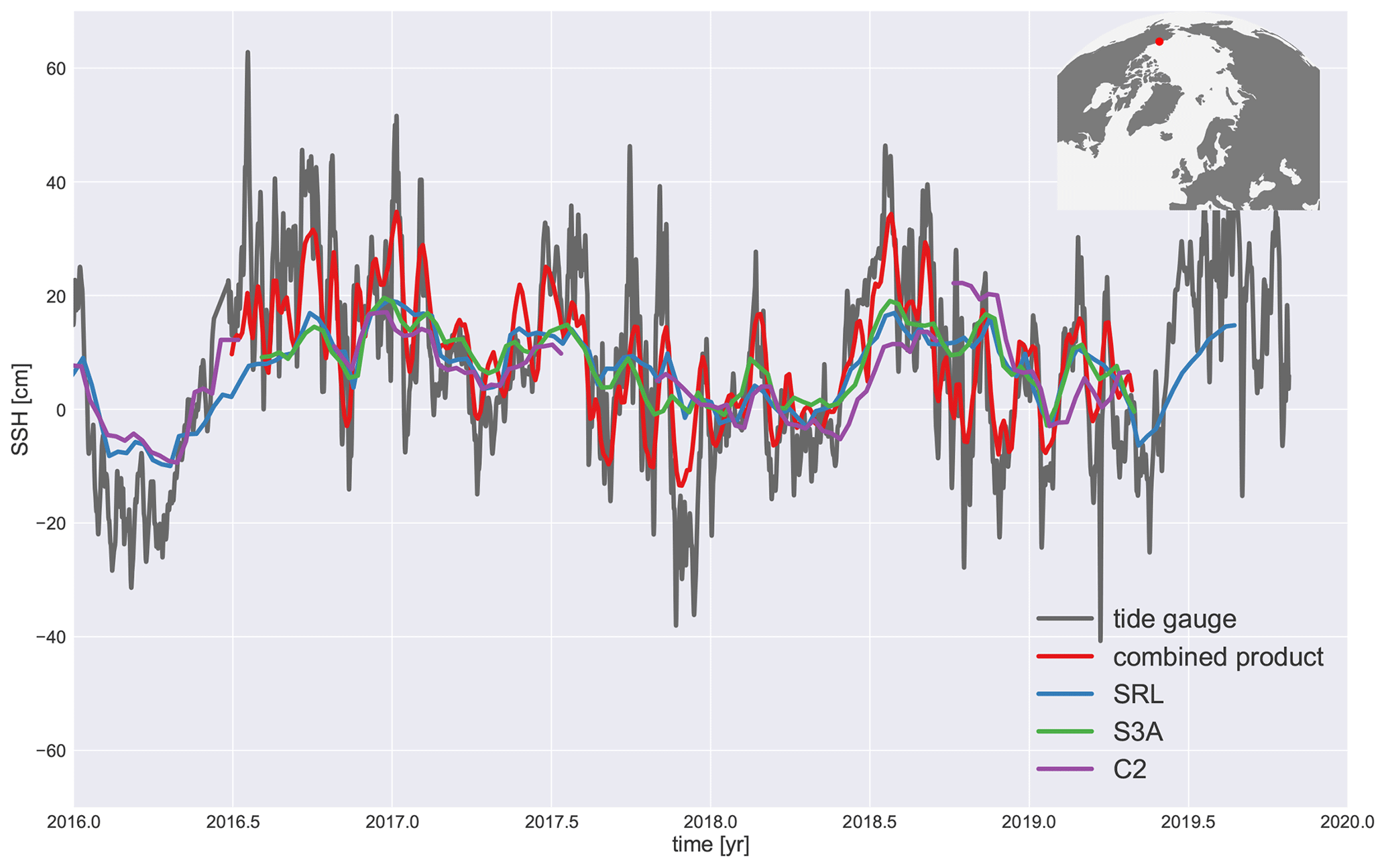
Figure 9Sea level anomaly time series at station Prudhoe Bay from the tide gauge station (dark gray), the combined altimetry product (red) and mono-mission sea levels for SRL (blue), S3A (green) and C2 (purple). SSH signifies sea surface height.
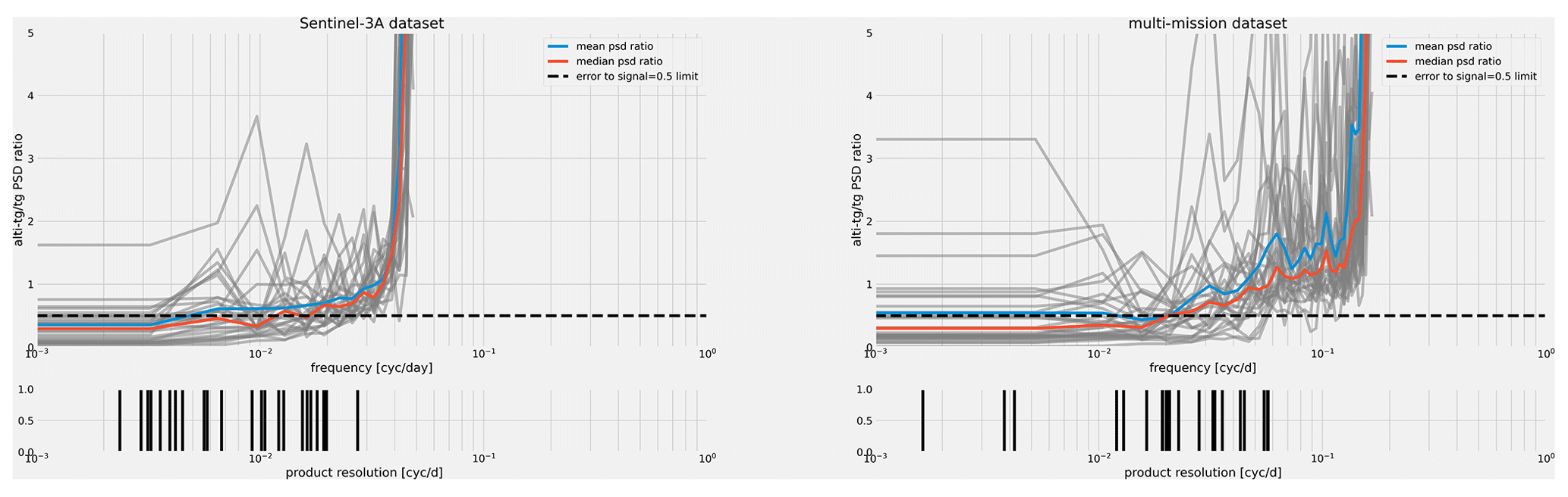
Figure 10Ratio of the error power spectrum to the signal power spectrum at tide gauges (gray lines); the mean (blue) and median (red) ratios are shown. The resolution threshold is displayed as a dashed black line. Resolution values are displayed (in cycles per day) in the bottom panels. The left panel is for a single altimeter (S3A) product and the right panel for the combined product. In the legend, psd signifies power spectral density.
4.4 Comparisons to tide gauges
Tide gauges provide an independent measurements of SL variability and are very valuable for the validation of satellite altimetry products (e.g., Cipollini et al., 2016). They are relatively scarce in the Arctic Ocean. Here we use data from the GLOSS/CLIVAR (Global Sea Level Observing System/Climate and Ocean – Variability, Predictability, and Change) tide gauge dataset from the University of Hawaii Sea Level Center (UHSLC) (Caldwell et al., 2010). Hourly tide gauge time series are de-tided using a Demerliac filter, corrected for dynamical atmospheric effects using the MOG2D model (Carrère and Lyard, 2003) and from glacial isostatic adjustment effects using the ICE5G-VM2 model (Peltier, 2004). A total of 27 stations are left after removal of records with obvious issues or large data gaps. Co-location with the altimetry dataset is performed by averaging altimeter grid points within 50 km (multi-mission data) or 150 km (mono-mission data) of the tide gauge position. Table 5 summarizes the correlations and root-mean-square deviation (RMSd) of altimetry and in situ SL differences for the combined product and for the three mono-mission products. For the combined product, the mean correlation across all stations is 0.78, and the mean RMSd is 5.3 cm, indicating an excellent agreement between tide gauge and altimeter data. The combined product performs better than any mono-mission product, indicating that the product accuracy benefits from the multi-mission combination.
To illustrate the level of agreement between altimetry and tide gauges, the Prudhoe Bay station records are shown in Fig. 9. Prudhoe Bay is one of the few stations providing high-quality tide gauge data in an area that is seasonally ice covered. At this station, where the ocean is seasonally ice covered, there is a good agreement between the tide gauge and all satellite radar altimeter products (mono-mission and combined). However, the combined product is able to capture the high-frequency SL variability observed by the tide gauge much better than any single altimeter product.
We also use tide gauges records to estimate the effective temporal resolution of the altimeter product following Ballarotta et al. (2019). Let the product error be the altimeter minus tide gauge SL differences, while the true signal is given by the tide gauge record. Then the product resolution corresponds to the frequency at which the error spectrum becomes greater than half the signal spectrum. Results are summarized in Fig. 10 The spread of the spectrum ratio remains large as the time span available is limited to 3 years. However, the improvement in resolution from a single altimeter product to a combined one is large. At best the resolution of the S3A-only product is around 3 months. For the combined product resolution can be as low as 1.5 months.
The different gridded datasets described in this paper are freely available, after registration, on the AVISO website (https://www.aviso.altimetry.fr/, last access: 19 November 2021) at https://doi.org/10.24400/527896/a01-2020.001 (Prandi, 2020).
Tide gauge data used in this study were retrieved from the UHSLC data portal at http://uhslc.soest.hawaii.edu/data/ (last access: 20 November 2021) (Caldwell et al., 2010, https://doi.org/10.7289/V5V40S7W).
In this paper, we document a new Arctic Ocean sea level dataset based on the combination of measurements from three satellite radar altimetry missions: SARAL/AltiKa, CryoSat-2 and Sentinel-3A. The processing applied to those three missions is described, as well as the optimal interpolation scheme used to create sea level anomaly fields.
Combined sea level anomaly and absolute dynamic topography fields are available over 3 years (from July 2016 to April 2019) on a 25 km grid, every 3 d, for all latitudes greater than 50∘ N. Temporal extensions are planned to increase the time span of the dataset. Comparisons to the DUACS global product suggest that despite focusing on high latitudes and ice-covered areas, the product performs well in permanently open ocean areas at lower latitudes. This dataset already helped support the existence of newly developing water pathways north of Svalbard (Athanase et al., 2021). Comparisons with tide gauges available in the Arctic Ocean show that the combined product is able to capture some of the high-frequency sea level variability observed by tide gauges and generally performs better than any of our single-altimeter analyses.
This unprecedented resolution may be useful for the characterization of small-scale Arctic Ocean circulation features.
PP generated the dataset, and JCP provided algorithms and advice for waveform processing. GD and YF helped with the multi-mission combination. AG led the project for CNES. All authors contributed to the manuscript.
The authors declare that they have no conflict of interest.
Publisher's note: Copernicus Publications remains neutral with regard to jurisdictional claims in published maps and institutional affiliations.
The work presented here was performed within the frame of the CNES Alti-Doppler Glaciologie contract. Radar altimeter data were provided by CNES (SARAL/AltiKA, Sentinel-3A) and ESA (CryoSat-2).
This paper was edited by Giuseppe M. R. Manzella and reviewed by two anonymous referees.
Andersen, O., Stenseng, L., Piccioni, G., and Knudsen, P.: The DTU15 MSS (Mean Sea Surface) and DTU15LAT (Lowest Astronomical Tide) reference surface, DTU Space, available at: ftp://ftp.space.dtu.dk/pub/DTU15/DOCUMENTS/MSS/DTU15MSS+LAT.pdf (last access: 19 November 2021), 2016. a, b, c
Armitage, T. W. K. and Davidson, M. W. J.: Using the Interferometric Capabilities of the ESA CryoSat-2 Mission to Improve the Accuracy of Sea Ice Freeboard Retrievals, IEEE T. Geosci. Remote, 52, 529–536, 2014. a
Armitage, T. W. K., Bacon, S., Ridout, A. L., Thomas, S. F., Aksenov, Y., and Wingham, D. J.: Arctic sea surface height variability and change from satellite radar altimetry and GRACE, 2003–2014, J. Geophys. Res.-Oceans, 121, 4303–4322, https://doi.org/10.1002/2015JC011579, 2016. a, b, c, d, e, f, g, h, i
Armitage, T. W. K., Bacon, S., Ridout, A. L., Petty, A. A., Wolbach, S., and Tsamados, M.: Arctic Ocean surface geostrophic circulation 2003–2014, The Cryosphere, 11, 1767–1780, https://doi.org/10.5194/tc-11-1767-2017, 2017. a
Athanase, M., Provost, C., Artana, C., Pérez-Hernández, M. D., Sennéchael, N., Bertosio, C., Garric, G., Lellouche, J.-M., and Prandi, P.: Changes in Atlantic Water Circulation Patterns and Volume Transports North of Svalbard Over the Last 12 Years (2008–2020), J. Geophys. Res.-Oceans, 126, e2020JC016825, https://doi.org/10.1029/2020jc016825, 2021. a
Ballarotta, M., Ubelmann, C., Pujol, M.-I., Taburet, G., Fournier, F., Legeais, J.-F., Faugère, Y., Delepoulle, A., Chelton, D., Dibarboure, G., and Picot, N.: On the resolutions of ocean altimetry maps, Ocean Sci., 15, 1091–1109, https://doi.org/10.5194/os-15-1091-2019, 2019. a
Boergens, E., Dettmering, D., Schwatke, C., and Seitz, F.: Treating the Hooking Effect in Satellite Altimetry Data: A Case Study along the Mekong River and Its Tributaries, Remote Sens.-Basel, 8, 91, https://doi.org/10.3390/rs8020091, 2016. a
Boy, F., Desjonqueres, J.-D., Picot, N., Moreau, T., and Raynal, M.: CryoSat-2 SAR-Mode Over Oceans: Processing Methods, Global Assessment, and Benefits, IEEE Transactions on Geoscience and Remote Sens.-Basel, 55, 148–158, https://doi.org/10.1109/tgrs.2016.2601958, 2017. a
Bretherton, F. P., Davis, R. E., and Fandry, C.: A technique for objective analysis and design of oceanographic experiments applied to MODE-73, Deep-Sea Research and Oceanographic Abstracts, 23, 559–582, https://doi.org/10.1016/0011-7471(76)90001-2, 1976. a
Brodzik, M. J., Billingsley, B., Haran, T., Raup, B., and Savoie, M.: Correction: Brodzik, M. J., et al. EASE-Grid 2.0: Incremental but Significant Improvements for Earth-Gridded Data Sets, ISPRS Int. J. Geo-Inf. 2012, 1, 32–45, ISPRS Int. J. Geo-Inf., 3, 1154–1156, https://doi.org/10.3390/ijgi3031154, 2014. a
Brodzik, M. J., Billingsley, B., Haran, T., Raup, B., and Savoie, M. H.: EASE-Grid 2.0: Incremental but Significant Improvements for Earth-Gridded Data Sets, ISPRS Int. J. Geo-Inf., 1, 32–45, https://doi.org/10.3390/ijgi1010032, 2012. a
Caldwell, P. C., Merrifield, M. A., and Thompson, P. R.: Sea level measured by tide gauges from global oceans as part of the Joint Archive for Sea Level (JASL) since 1846, NOAA National Centers For Environmental Information [data set], https://doi.org/10.7289/V5V40S7W, 2010 (data available at: http://uhslc.soest.hawaii.edu/data/, last access: 20 November 2021). a, b
Carrère, L. and Lyard, F.: Modeling the barotropic response of the global ocean to atmospheric wind and pressure forcing – comparisons with observations, Geophys. Res. Lett., 30, 1275, https://doi.org/10.1029/2002gl016473, 2003. a, b
Carrère, L., Lyard, F., Cancet, M., Guillot, A., and Picot, N.: FES 2014, a new tidal model – Validation results and perspectives for improvements, ESA Living Planet Symposium, 2016. a
Cartwright, D. E. and Edden, A. C.: Corrected Tables of Tidal Harmonics, Geophys. J. Int., 33, 253–264, https://doi.org/10.1111/j.1365-246x.1973.tb03420.x, 1973. a
Chelton, D. B., Ries, J. C., Haines, B. J., Fu, L.-L., and Callahan, P. S.: Satellite Altimetry, Chapter 1, International Geophysics, 69, 1–131, i–ii, https://doi.org/10.1016/s0074-6142(01)80146-7, 2001. a
Cipollini, P., Calafat, F. M., Jevrejeva, S., Melet, A., and Prandi, P.: Monitoring Sea Level in the Coastal Zone with Satellite Altimetry and Tide Gauges, Surv. Geophys., 38, 33–57, https://doi.org/10.1007/s10712-016-9392-0, 2016. a
Danielson, S. L., Hennon, T. D., Hedstrom, K. S., Pnyushkov, A. V., Polyakov, I. V., Carmack, E., Filchuk, K., Janout, M., Makhotin, M., Williams, W. J., and Padman, L.: Oceanic Routing of Wind-Sourced Energy Along the Arctic Continental Shelves, Frontiers in Marine Science, 7, 509, https://doi.org/10.3389/fmars.2020.00509, 2020. a
Desai, S., Wahr, J., and Beckley, B.: Revisiting the pole tide for and from satellite altimetry, J. Geodesy, 89, 1233–1243, https://doi.org/10.1007/s00190-015-0848-7, 2015. a
Donlon, C., Berruti, B., Buongiorno, A., Ferreira, M.-H., Féménias, P., Frerick, J., Goryl, P., Klein, U., Laur, H., Mavrocordatos, C., Nieke, J., Rebhan, H., Seitz, B., Stroede, J., and Sciarra, R.: The Global Monitoring for Environment and Security (GMES) Sentinel-3 mission, Remote Sens. Environ., 120, The Sentinel Missions – New Opportunities for Science, 37–57, https://doi.org/10.1016/j.rse.2011.07.024, 2012. a
Ducet, N., Le Traon, P. Y., and Reverdin, G.: Global high-resolution mapping of ocean circulation from TOPEX/Poseidon and ERS-1 and -2, J. Geophys. Res.-Oceans, 105, 19477–19498, https://doi.org/10.1029/2000jc900063, 2000. a, b
Giles, K. a., Laxon, S. W., Ridout, A. L., Wingham, D. J., and Bacon, S.: Western Arctic Ocean freshwater storage increased by wind-driven spin-up of the Beaufort_Gyre, Nat. Geosci., 5, 194–197, https://doi.org/10.1038/ngeo1379, 2012. a, b
Helm, V., Humbert, A., and Miller, H.: Elevation and elevation change of Greenland and Antarctica derived from CryoSat-2, The Cryosphere, 8, 1539–1559, https://doi.org/10.5194/tc-8-1539-2014, 2014. a
Iijima, B., Harris, I., Ho, C., Lindqwister, U., Mannucci, A., Pi, X., Reyes, M., Sparks, L., and Wilson, B.: Automated daily process for global ionospheric total electron content maps and satellite ocean altimeter ionospheric calibration based on Global Positioning System data, J. Atmos. Sol.-Terr. Phy., 61, 1205–1218, https://doi.org/10.1016/s1364-6826(99)00067-x, 1999. a
Kwok, R.: Arctic sea ice thickness, volume, and multiyear ice coverage: losses and coupled variability (1958–2018), Environ. Res. Lett., 13, 105005, https://doi.org/10.1088/1748-9326/aae3ec, 2018. a
Lavergne, T., Sørensen, A. M., Kern, S., Tonboe, R., Notz, D., Aaboe, S., Bell, L., Dybkjær, G., Eastwood, S., Gabarro, C., Heygster, G., Killie, M. A., Brandt Kreiner, M., Lavelle, J., Saldo, R., Sandven, S., and Pedersen, L. T.: Version 2 of the EUMETSAT OSI SAF and ESA CCI sea-ice concentration climate data records, The Cryosphere, 13, 49–78, https://doi.org/10.5194/tc-13-49-2019, 2019. a
Lawrence, I. R., Armitage, T. W., Tsamados, M. C., Stroeve, J. C., Dinardo, S., Ridout, A. L., Muir, A., Tilling, R. L., and Shepherd, A.: Extending the Arctic sea ice freeboard and sea level record with the Sentinel-3 radar altimeters, Adv. Space Res., 68, 711–723, https://doi.org/10.1016/j.asr.2019.10.011, 2019. a
Le Traon, P. Y. and Dibarboure, G.: Mesoscale Mapping Capabilities of Multiple-Satellite Altimeter Missions, J. Atmos. Ocean. Tech., 16, 1208–1223, https://doi.org/10.1175/1520-0426(1999)016<1208:mmcoms>2.0.co;2, 1999. a, b
Le Traon, P.-Y. and Ogor, F.: ERS-1/2 orbit improvement using TOPEX/POSEIDON: The 2 cm challenge, J. Geophys. Res.-Oceans, 103, 8045–8057, https://doi.org/10.1029/97jc01917, 1998. a
Longépé, N., Thibaut, P., Vadaine, R., Poisson, J., Guillot, A., Boy, F., Picot, N., and Borde, F.: Comparative Evaluation of Sea Ice Lead Detection Based on SAR Imagery and Altimeter Data, IEEE T. Geosci. Remote, 57, 4050–4061, https://doi.org/10.1109/TGRS.2018.2889519, 2019. a, b
Meredith, M., Sommerkorn, M., Cassotta, S., Derksen, C., Ekaykin, A., Hollowed, A., Kofinas, G., Mackintosh, A., Melbourne-Thomas, J., Muelbert, M., Ottersen, G., Pritchard, H., and Schuur, E.: Polar Regions, Cahp. 3, IPCC's Special Report on the Ocean and Cryosphere in a Changing Climate, 2019. a
Müller, F., Dettmering, D., Bosch, W., and Seitz, F.: Monitoring the Arctic Seas: How Satellite Altimetry Can Be Used to Detect Open Water in Sea-Ice Regions, Remote Sens.-Basel, 9, 551, https://doi.org/10.3390/rs9060551, 2017. a
Pascual, A., Faugère, Y., Larnicol, G., and Le Traon, P. Y.: Improved description of the ocean mesoscale variability by combining four satellite altimeters, Geophys. Res. Lett., 33, L02611, https://doi.org/10.1029/2005GL024633, 2006. a, b
Peacock, N. R. and Laxon, S.: Sea surface height determination in the Arctic Ocean from ERS altimetry, J. Geophys. Res., 109, C07001, https://doi.org/10.1029/2001JC001026, 2004. a, b, c
Peltier, W.: GLOBAL GLACIAL ISOSTASY AND THE SURFACE OF THE ICE-AGE EARTH: The ICE-5G (VM2) Model and GRACE, Annu. Rev. Earth Pl. Sc., 32, 111–149, https://doi.org/10.1146/annurev.earth.32.082503.144359, 2004. a
Poisson, J., Quartly, G. D., Kurekin, A. A., Thibaut, P., Hoang, D., and Nencioli, F.: Development of an ENVISAT Altimetry Processor Providing Sea Level Continuity Between Open Ocean and Arctic Leads, IEEE T. Geosci. Remote, 56, 5299–5319, 2018. a, b, c
Polyakov, I. V., Pnyushkov, A. V., Alkire, M. B., Ashik, I. M., Baumann, T. M., Carmack, E. C., Goszczko, I., Guthrie, J., Ivanov, V. V., Kanzow, T., Krishfield, R., Kwok, R., Sundfjord, A., Morison, J., Rember, R., and Yulin, A.: Greater role for Atlantic inflows on sea-ice loss in the Eurasian Basin of the Arctic Ocean, Science, 356, 285–291, https://doi.org/10.1126/science.aai8204, 2017. a
Prandi, P.: Gridded Sea Level Heights – Arctic Ocean, AVISO+ [data set], https://doi.org/10.24400/527896/a01-2020.001, 2020 (data available at: https://www.aviso.altimetry.fr/, last access: 19 November 2021). a, b
Proshutinsky, A., Dukhovskoy, D., Timmermans, M.-L., Krishfield, R., and Bamber, J. L.: Arctic circulation regimes, Philos. T. R. Soc. A, 373, 20140160, https://doi.org/10.1098/rsta.2014.0160, 2015. a
Pujol, M.-I., Faugère, Y., Taburet, G., Dupuy, S., Pelloquin, C., Ablain, M., and Picot, N.: DUACS DT2014: the new multi-mission altimeter data set reprocessed over 20 years, Ocean Sci., 12, 1067–1090, https://doi.org/10.5194/os-12-1067-2016, 2016. a
Pujol, M.-I., Schaeffer, P., Faugère, Y., Raynal, M., Dibarboure, G., and Picot, N.: Gauging the Improvement of Recent Mean Sea Surface Models: A New Approach for Identifying and Quantifying Their Errors, J. Geophys. Res.-Oceans, 123, 5889–5911, https://doi.org/10.1029/2017jc013503, 2018. a
Quartly, G., Rinne, E., Passaro, M., Andersen, O., Dinardo, S., Fleury, S., Guillot, A., Hendricks, S., Kurekin, A., Müller, F., Ricker, R., Skourup, H., and Tsamados, M.: Retrieving Sea Level and Freeboard in the Arctic: A Review of Current Radar Altimetry Methodologies and Future Perspectives, Remote Sens.-Basel, 11, 881, https://doi.org/10.3390/rs11070881, 2019. a, b
Regan, H., Lique, C., Talandier, C., and Meneghello, G.: Response of total and eddy kinetic energy to the recent spinup of the Beaufort Gyre, J. Phys. Oceanogr., 50, 575–594, https://doi.org/10.1175/JPO-D-19-0234.1, 2020. a
Regan, H. C., Lique, C., and Armitage, T. W. K.: The Beaufort Gyre Extent, Shape, and Location Between 2003 and 2014 From Satellite Observations, J. Geophys. Res.-Oceans, 124, 844–862, https://doi.org/10.1029/2018JC014379, 2019. a
Rose, S. K., Andersen, O. B., Passaro, M., Ludwigsen, C. A., and Schwatke, C.: Arctic Ocean Sea Level Record from the Complete Radar Altimetry Era: 1991–2018, Remote Sens.-Basel, 11, 1672, https://doi.org/10.3390/rs11141672, 2019. a, b, c, d, e, f
Smith, G. C., Allard, R., Babin, M., Bertino, L., Chevallier, M., Corlett, G., Crout, J., Davidson, F., Delille, B., Gille, S. T., Hebert, D., Hyder, P., Intrieri, J., Lagunas, J., Larnicol, G., Kaminski, T., Kater, B., Kauker, F., Marec, C., Mazloff, M., Metzger, E. J., Mordy, C., OCarroll, A., Olsen, S. M., Phelps, M., Posey, P., Prandi, P., Rehm, E., Reid, P., Rigor, I., Sandven, S., Shupe, M., Swart, S., Smedstad, O. M., Solomon, A., Storto, A., Thibaut, P., Toole, J., Wood, K., Xie, J., Yang, Q., and the WWRP PPP Steering Group: Polar Ocean Observations: A Critical Gap in the Observing System and Its Effect on Environmental Predictions From Hours to a Season, Frontiers in Marine Science, 6, 429, https://doi.org/10.3389/fmars.2019.00429, 2019. a, b
Smith, W. H. F. and Scharroo, R.: Waveform Aliasing in Satellite Radar Altimetry, IEEE T. Geosci. Remote, 53, 1671–1682, https://doi.org/10.1109/TGRS.2014.2331193, 2015. a
Stammer, D. and Cazenave, A. (Eds.): Satellite Altimetry Over Oceans and Land Surfaces, CRC Press, Boca Raton, https://doi.org/10.1201/9781315151779, 2018. a
Steunou, N., Desjonquères, J. D., Picot, N., Sengenes, P., Noubel, J., and Poisson, J. C.: AltiKa Altimeter: Instrument Description and In Flight Performance, Mar. Geod., 38, 22–42, https://doi.org/10.1080/01490419.2014.988835, 2015. a
Stroeve, J. and Notz, D.: Changing state of Arctic sea ice across all seasons, Environ. Res. Lett., 13, 103001, https://doi.org/10.1088/1748-9326/aade56, 2018. a
Taburet, G., Sanchez-Roman, A., Ballarotta, M., Pujol, M.-I., Legeais, J.-F., Fournier, F., Faugere, Y., and Dibarboure, G.: DUACS DT2018: 25 years of reprocessed sea level altimetry products, Ocean Sci., 15, 1207–1224, https://doi.org/10.5194/os-15-1207-2019, 2019. a, b, c, d
Timmermans, M.-L., Ladd, C., and Wood, K.: Sea surface temperature, Arctic Report Card, available at: https://arctic.noaa.gov/Report-Card/Report-Card-2017/ArtMID/7798/ArticleID/698/Sea-Surface-Temperature (last access: 20 November 2021), 2017. a
Valladeau, G., Thibaut, P., Picard, B., Poisson, J. C., Tran, N., Picot, N., and Guillot, A.: Using SARAL/AltiKa to Improve Ka-band Altimeter Measurements for Coastal Zones, Hydrology and Ice: The PEACHI Prototype, Mar. Geod., 38, 124–142, https://doi.org/10.1080/01490419.2015.1020176, 2015. a
Verron, J., Sengenes, P., Lambin, J., Noubel, J., Steunou, N., Guillot, A., Picot, N., Coutin-Faye, S., Sharma, R., Gairola, R. M., Murthy, D. V. A. R., Richman, J. G., Griffin, D., Pascual, A., Rémy, F., and Gupta, P. K.: The SARAL/AltiKa Altimetry Satellite Mission, Mar. Geod., 38, 2–21, https://doi.org/10.1080/01490419.2014.1000471, 2015. a
Wingham, D., Francis, C., Baker, S., Bouzinac, C., Brockley, D., Cullen, R., de Chateau-Thierry, P., Laxon, S., Mallow, U., Mavrocordatos, C., Phalippou, L., Ratier, G., Rey, L., Rostan, F., Viau, P., and Wallis, D.: CryoSat: A mission to determine the fluctuations in Earth's land and marine ice fields, Adv. Space Res., 37, 841–871, https://doi.org/10.1016/j.asr.2005.07.027, 2006. a
Zhao, M., Timmermans, M.-L., Cole, S., Krishfield, R., and Toole, J.: Evolution of the eddy field in the Arctic Ocean's Canada Basin, 2005–2015, Geophys. Res. Lett., 43, 8106–8114, https://doi.org/10.1002/2016GL069671, 2016. a