the Creative Commons Attribution 4.0 License.
the Creative Commons Attribution 4.0 License.
 | 18 Nov 2021
The first global 883 GHz cloud ice survey: IceCube Level 1 data calibration, processing and analysis
Dong L. Wu
Patrick Eriksson
Sub-millimeter (200–1000 GHz) wavelengths contribute a unique capability to fill in the sensitivity gap between operational visible–infrared (VIS–IR) and microwave (MW) remote sensing for atmospheric cloud ice and snow. Being able to penetrate clouds to measure cloud ice mass and microphysical properties in the middle to upper troposphere, a critical spectrum range, is necessary for us to understand the connection between cloud ice and precipitation processes.
As the first spaceborne 883 GHz radiometer, the IceCube mission was NASA's latest spaceflight demonstration of commercial sub-millimeter radiometer technology. Successfully launched from the International Space Station, IceCube is essentially a free-running radiometer and collected valuable 15-month measurements of atmosphere and cloud ice. This paper describes the detailed procedures for Level 1 (L1) data calibration, processing and validation. The scientific quality and value of IceCube data are then discussed, including radiative transfer model validation and evaluation, as well as the unique spatial distribution and diurnal cycle of cloud ice that are revealed for the first time on a quasi-global scale at this frequency. IceCube Level 1 dataset is publicly available at Gong and Wu (2021) (https://doi.org/10.25966/3d2p-f515).
- Article
(6928 KB) - Full-text XML
- BibTeX
- EndNote


Ice clouds play a crucial role in Earth’s climate and weather through interactions with atmospheric radiation, dynamics and precipitation processes at a wide range of spatial and temporal scales (Wu et al., 2019). By far ice clouds remain the leading source of uncertainty in weather model predictions and future climate projections (Stocker et al., 2013) mainly because of two reasons. On the one hand, upper-tropospheric ice clouds are radiatively important to Earth’s energy budget, and inaccurate measurements of ice cloud properties add poor or even misleading constraints on ice cloud radiative feedback (CRF) in models. On the other hand, large ice crystals fall and form precipitation eventually. Traditional remote sensing techniques leave gaps in this cloud–precipitation transition and coupling process. As a result, ice cloud and associated radiative and hydrological properties simulated by general circulation models (GCMs) vary wildly and are often subjected to heavy tuning to close the radiation budget at the top of the atmosphere and precipitation at the surface, leaving the middle of the process highly uncertain and underconstrained (Waliser et al., 2009; Li et al., 2016).
Ice clouds' net radiative effect can be positive or negative depending on its macrophysical (e.g., cloud top height and optical thickness) and microphysical (e.g., particle size distribution and particle shape) properties. Large discrepancies still remain among various satellite ice cloud retrieval products and between observations and reanalyses and/or GCM simulations. Traditional remote sensing techniques working at visible (VIS) and infrared (IR) spectrum ranges are sensitive to ice cloud properties such as cloud top height, optical thickness, particle size, etc. (Wang et al., 2016) but suffer from only being able to penetrate the top few kilometers of the cloud layer (Eliasson et al., 2011). For example, Eliasson et al. (2011) and Duncan and Eriksson (2018) identified more than 300 % discrepancies among ice water path (IWP) retrievals derived from different A-Train satellite instruments, although they all sample the same body of cloud at the same local time.
Moreover, achieving consensus about ice cloud mass is unavoidably a critical step when attempting to close the global hydrological budget. Unfortunately the aforementioned sensitivity gap between the VIS–IR and MW (microwave) measurements results in the missing piece of the inter-coupled process that connects atmospheric clouds with precipitation-sized hydrometers. Although combined spaceborne radar and lidar observations (e.g., DARDAR – radar lidar – or 2C-ICE – CloudSat and CALIPSO (Cloud-Aerosol Lidar and Infrared Pathfinder Satellite Observation) Ice Cloud Property Product – products) largely alleviated this problem, they are not suitable for capturing daily weather-scale variabilities because of narrow swaths and infrequent revisit times. Relatively inexpensive passive sensors are still required to cover the wide spatial and temporal scales of weather as well as to produce the climate record.
The sensitivity gap is visually quantified in Fig. 1a. In this figure, the two-dimensional probability density functions (PDFs) between Tcir and IWP are constructed based on pure observations from a passive infrared sensor (Atmospheric Infrared Sounder, or AIRS) and a passive-microwave sensor (Microwave Humidity Sounder, or MHS), respectively. Tcir, the so-called “cloud-induced radiance depression”, is defined as the difference between the observed brightness temperature (TB) and the simulated clear-sky radiance (Tccr) by removing any frozen hydrometeors from the column (Gong and Wu, 2014; Wu et al., 2019). IWP “truth” is extracted from the joint spaceborne radar and lidar product called 2C-ICE, and Tcir values are taken from collocated IR and MW observations, respectively. From Fig. 1a we can see the sensitivity range, where the slope is steep enough to be estimated, is about 10–70 g m−2 for passive IR sensors; however, Tcir for a typical passive MW sensor does not start to become sensitive to IWP before it exceeds 300 g m−2 or so, as marked by the horizontal rectangles in Fig. 1a. The sensitivity range for IceCube, based on a radiative transfer model simulation (blue curve), is between 40 and 600 g m−2, which perfectly fills in the gap between IR and MW sensors (orange rectangles). Readers are directed to Appendix A for details of observational datasets, collocation algorithm and model simulations. Hence, we add the sub-millimeter (sub-mm) sensitivity column (blue cylinder) in Fig. 1 of Eliasson et al. (2011), as shown here in Fig. 1b. Admittedly the VIS–IR spectrum (yellow cylinder) could largely cover the same sensitivity range of the sub-millimeter spectrum, but visible spectrum loses its capability at nighttime and during the polar night season and furthermore suffers from multiple scattering to small ice crystals.

Figure 1(a) Two-dimensional probability density functions (PDFs) of cloud-induced radiance perturbation (Tcir) and ice water path (IWP) derived from collocated CloudSat–CALIPSO and AIRS (color shaded) and MHS (color contours) observations in the tropics (30∘ S–30∘ N). The blue solid line connects the PDF peak for AIRS and CloudSat–CALIPSO. Black solid (dashed) line is from the ARTS model simulation for 874 (190) GHz. See Appendix A for details. (b) A conceptual depiction of the rough penetration depth of different passive and active spaceborne sensors. This panel is modified from Fig. 1 in Eliasson et al. (2011) by adding the sub-millimeter sensitivity column (blue).
The 874 GHz channel (or more generally speaking, 860–900 GHz range) not only provides great sensitivity to cloud ice scattering but also allows for sufficient penetration to measure upper–middle-tropospheric cloud ice mass and size properties. Gruntzun et al. (2018) found out that the sensitivity level to cloud (snow) ice peaks at ∼300 hPa (400 hPa) for 874 GHz at the nadir view using the Atmospheric Radiative Transfer Simulator (ARTS) and its comprehensive ice scattering database and absorption spectrum (Buehler et al., 2018). This channel also has a strong positive response at about 200–300 hPa to water vapor, meaning that it can be merely contaminated by complicated surface signals or liquid/rain clouds in the lower troposphere, unless the upper troposphere is extremely dry. Since it is relatively easy to obtain water vapor information in the upper troposphere (e.g., Moradi et al., 2015; Bosilovich et al., 2017), 874 GHz is an ideal channel for retrieving ice cloud mass for medium-thick ice clouds located above 400 hPa. Moreover, radiative transfer model (RTM) simulations also indicate that this frequency is the most sensitive to ice particles with an effective diameter (De) between 100–200 µm (Buehler et al., 2007; Tang et al., 2015). While numerous studies have revealed that MW Mie scattering only happens for precipitation-sized particles (De>200 µm), the VIS channel sensitivity range is 10–120 µm (Platnick et al., 2017), and the IR sensitivity range is 20–100 µm (Garnier et al., 2013; Wang et al., 2016); 874 GHz fills in not only the sensitivity gap of ice cloud mass but also the gap of the ice particle size spectrum. Above that frequency at the THz band, cloud ice remote sensing becomes more difficult because of increasing atmospheric attenuation from the gas continuum absorption (Wu et al., 2019).
Working at 883 GHz with the lower sideband at 874 GHz, IceCube is one of the only three known instruments that were ever built to work at this frequency. Therefore, making IceCube data available to the public is of critical importance to benefit the entire scientific community to advance our understanding of ice cloud radiative feedback and cloud–precipitation coupling processes.
This paper is organized as follows. Section 2 describes the procedures for data calibration, gain model construction and geolocation registration. Section 3 validates the quality of the delivered Level 1 (L1) radiance data against other satellite datasets and previous campaign data collections as well as RTM simulations. Section 4 discusses some scientific applications of this dataset. Section 5 includes the conclusion and some discussion about future directions for instrument design and orbital selection.
The IceCube mission was funded by NASA to make a fast-track spaceflight demonstration and validation of the VDI (Virginia Diodes, Inc.) 883 GHz receiver for cloud ice observations. VDI’s commercialized 874 GHz receiver greatly reduced the cost of this mission, yet the stability of this receiver in space is uncertain. IceCube was successfully deployed from the International Space Station (ISS) on 16 May 2017 and re-entered Earth's atmosphere on 2 October 2018. During its ∼15 months of life in space, IceCube not only successfully completed its primary goal to retire the risks for the VDI receiver but also collected a large amount of scientifically valuable data over low latitudes to mid-latitudes that led the first-ever global cloud ice map at this frequency. This section is dedicated describing the procedures we carried out to deliver the Level 1 radiance data (Gong and Wu, 2021).
To reduce the mission risk and power usage, IceCube was chosen to fly without a scan mirror for radiometric calibration. Instead, it spins the spacecraft to obtain periodic views between cold space and Earth’s atmosphere. Thus, the cold-space count measurements and clear-sky Earth atmosphere are used for the radiometric calibration and receiver gain calculation. This simplified engineering design successfully kept the cost low but poses some challenges for the data calibration, geolocation registration and data processing. The IceCube antenna produces a 1.8∘ half-power beam width, which translates to a 12.6 km nadir footprint size at ISS orbit (∼400 km), which gradually decreased as the IceCube spacecraft dropped down to its orbit height. Interested readers are encouraged to read Wu et al. (2019) for more details regarding instrument design, altitude control, etc.
2.1 Cold-space calibration and offset
IceCube is essentially a free-running radiometer. As it lacks a stable cold/hot reference for absolute calibration, IceCube is calibrated against the predicted “space counts” in each spin, which should be calibrated to 0 all the time. Here “count” stands for the digitized number of voltage. The space count (Csp) is not a constant but a strong function of the receiver temperature (Tp) and the relative time duration with respect the most recent switch-on time (dt). A noise source injector is included, so the output voltage counts have four modes: antenna plus noise (Ant+N), antenna (Ant), reference (Ref) and reference plus noise (Ref+N). Adding noise is for testing the instrument calibration function, so the measured total voltage count (C) is defined as CAnt−CRef, where C is a function of Tp, as shown in Eq. (1):
Here Ce is the Earth-view counts. G is the instrument gain, which is also a function of Tp and Δt. The latter corresponds to the Julian day counted from 1 January 2017, as instrument gain is degrading slowly through time but is considered stable each day. Tb is the Level 1 radiance that we aim to get at the end. Rsp is the residual of Csp which could not be fitted by our space count fitting procedures. Four temperature readings were recorded, which are temperatures for the isolator (Tp1), detector (Tp2), reflector (Tp3) and mixer (Tp4). They are highly correlated, but as the mixer is closest to the output end, we use this record to represent Tp for the first two steps of calibration. Another three Tp measurements are used subsequently in the machine learning/artificial intelligence (ML/AI) training step to identify any trivial contributions to the unexplained residual.
To give an example, Fig. 2a plots the time series (with respect to the orbit switch-on time) of the raw counts (C) measurements. The first step shown in Fig. 2b is to apply a second-order polynomial fitting twice with respect to Tp4 to remove the temperature-dependent variation in Csp, which is successfully captured (red line). The second step is to remove the periodically varying component by a fifth-order polynomial fitting (blue line), which may be associated with IceCube location and/or spin velocity. The third step is to further remove the periodically varying component with respect to Tp3 and Tp4 by applying a sinusoidal fitting to Tp3 and then Tp4 (purple line), respectively. After removing this low-frequency component, the residual of Csp is about four counts for this case, and the Earth-view counts Ce now remain stable on this orbit and are clearly separated from the Csp. The fifth step is to separate them by detecting the sudden jumps along the time series, as shown by the blue and red crosses in Fig. 3. Once the jumping points are identified, the average time in between is considered the “nadir-view” time (indicated by thin black vertical lines). Now we can see “dips” in some segments of Ce in Fig. 3, e.g., the one at dt=710 s and the one at dt=1720 s. These dips are induced by cloud scattering.
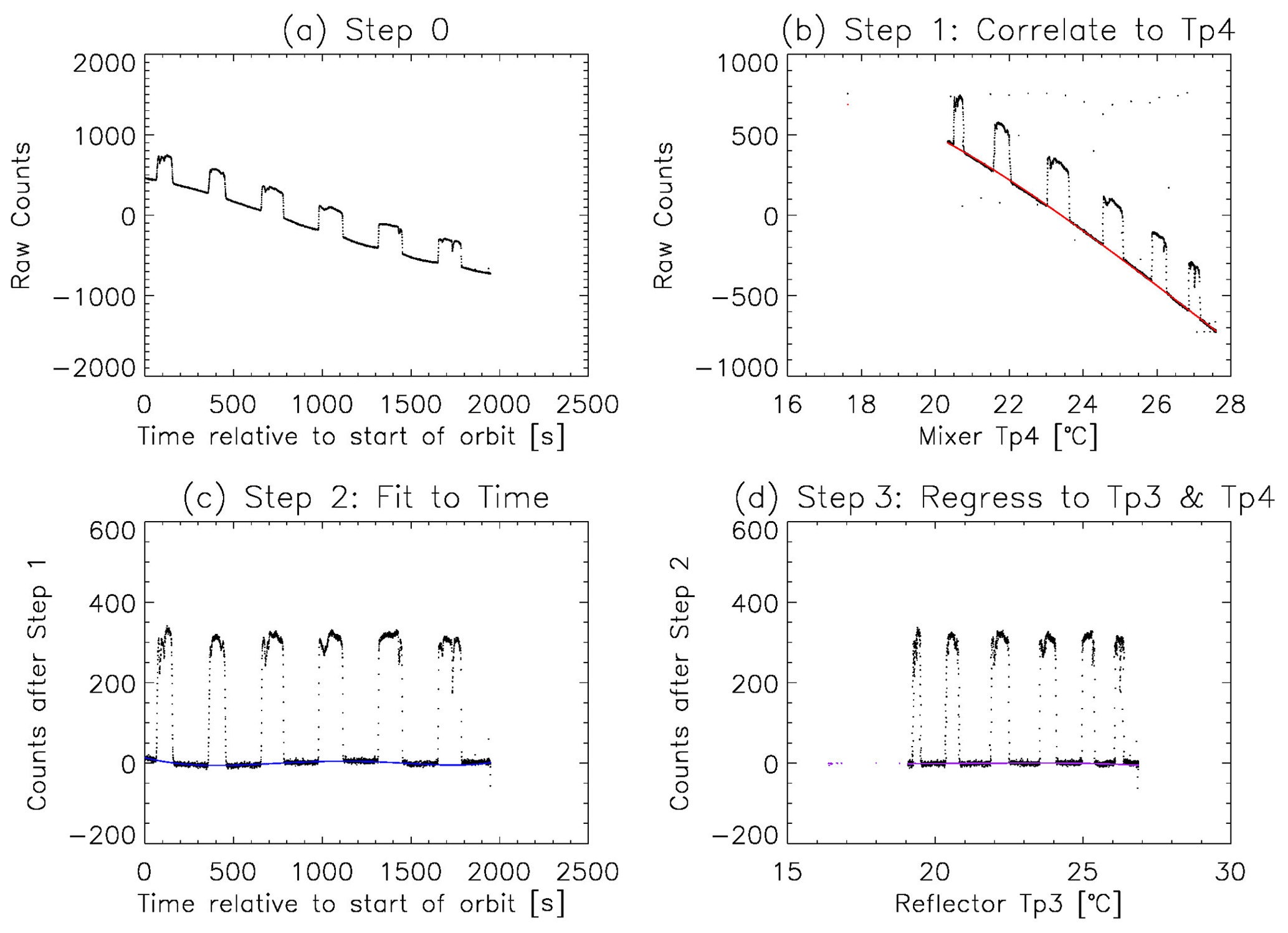
Figure 2An example showing the four steps of relative calibration: (a) raw total counts (C), (b) raw counts polynomial fitting to Tp4 (red) can largely capture the Csp variation, (c) count residuals polynomial fitting to relative time (blue), and (d) count residuals polynomial fitting to Tp3 and Tp4 (purple). After these four steps, standard deviation of Csp decreased to about four counts. This orbit is taken from the first orbit of IceCube on 14 August 2017.
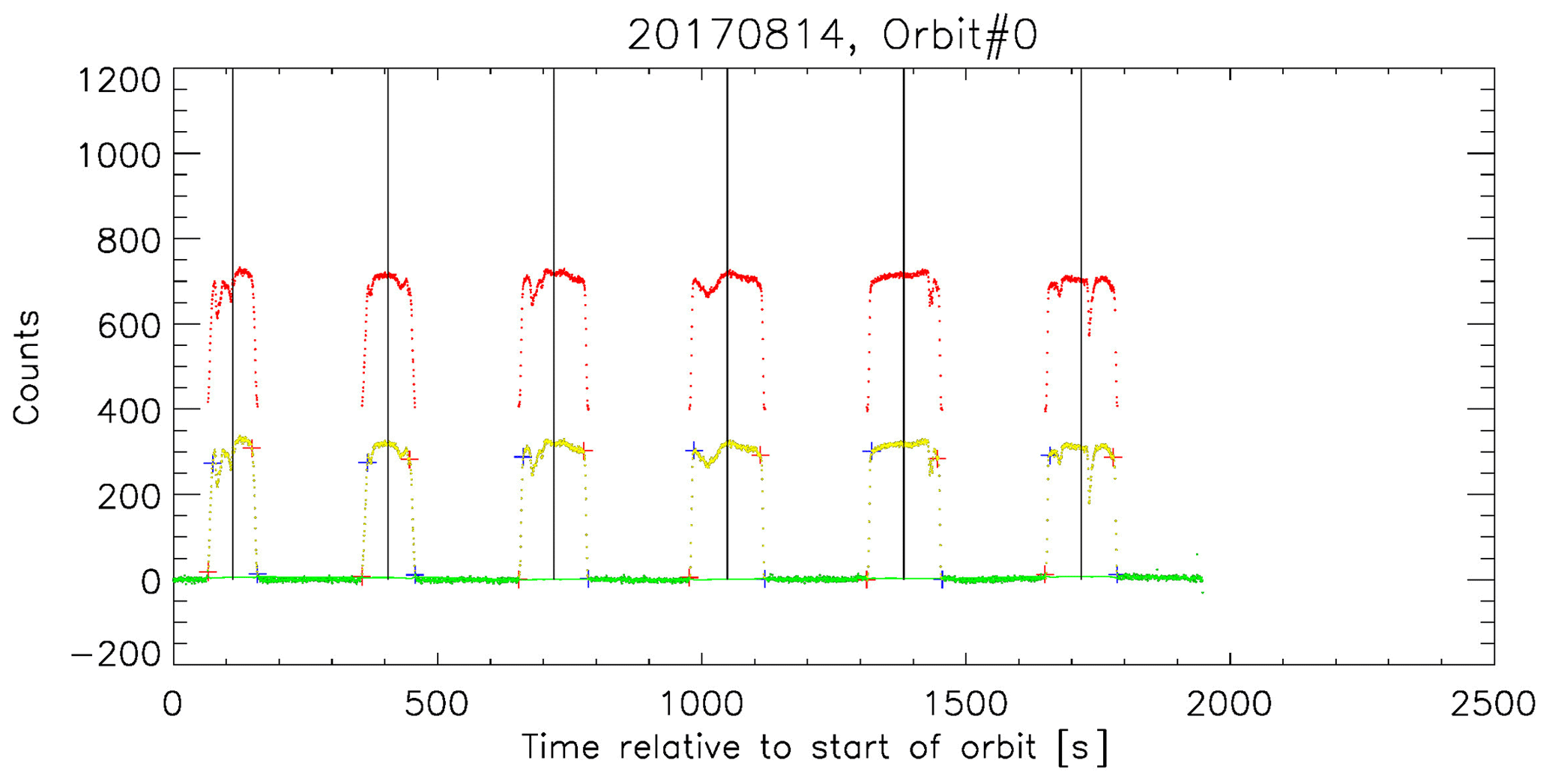
Figure 3Further separation of space view (green) and Earth view (yellow) by detecting the jumping thresholds (blue and red crosses). After separating the views, Csp was further fitted again by a polynomial fitting to remove slowly varying component. The red dots (shifted upward by 200 counts) are the final Earth voltage counts that will be converted to TB. This final polynomial fitting seems redundant here for a good orbit but is quite necessary for a bad orbit, an example of which is given in Appendix B. The average time between the starting and ending times of each Earth-view spin is assigned as the nadir-view time (thin black vertical lines). Please note that the date format in this figure is year month day.
However, it turned out that steps 3 and 4 may not remove all slowly varying Csp components, as suggested by a “bad example” in Appendix B. Therefore, a further polynomial fit is carried out (green thin line in Fig. 3) to secure the stability of Ce. In this final step, the spin velocity is calculated and compared to the recorded angular velocity. If the spin velocity is too slow or if the contrast between the adjacent Ce and Csp is too small, this spin is considered of poor quality and is entirely excluded from the final Level 1 product (see Appendix B for examples).
The residual (Rsp) (i.e., difference between the green dots and the green line on Fig. 3) provides a good estimate of the noise level of Ce, which remains ∼4 K throughout the mission (black crosses in Fig. 4). Since only dt, Tp3 and Tp4 are used for the empirical calibration of steps 1–5, an ML/AI model was trained and used as the final step to check whether the noise (σsp) can be further reduced. Here σsp is defined as the standard deviation of the residual Rsp. After applying this model, σsp indeed was reduced to ∼2 K as shown by the red crosses in Fig. 4. While details of the ML/AI model can be found in Appendix C, this exercise is somewhat illuminating to the engineering team: ML/AI may serve as a general and cost-effective calibration approach for any instrument to combat after-deployment variations that are not well understood in the pre-launch phase and can be relatively easily carried over to a constellation of CubeSats/microsatellites.
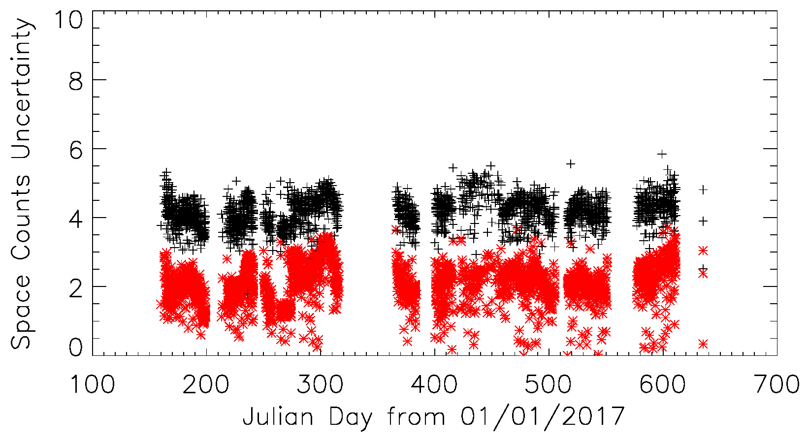
Figure 4Time series of σsp before the ML/AI model fitting (black crosses) and after the fitting (red crosses). Each cross represents one orbit.
2.2 Viewing angle and geolocation registration
IceCube essentially flies on the same orbit as the ISS. However, due to its free-spinner design, its latitude coverage can reach up to 58∘ N/S. Spin rate is a critical parameter in order to accurately register the geolocation of an observation. Spin rate in the unit of degrees per second (dps) is the second-tier variable to determine. In addition, because geolocation is necessary for the calculation of clear-sky radiance Tccr, which is used for constructing the gain model as well as for the IWP retrieval, spin rate is subsequently a must.
IceCube has three spinning modes. In the daytime, it spun around the sun vector (−y axis) at the sun point (SP) mode (−1 dps) or fine reference point (FRP) mode (−1.2 dps). At nighttime, it spun around the geomagnetic field (+z axis) at a speed between +1 to +2 dps. Three axis spin rates are recorded as spinx, spiny and spinz. However, the observed spin rate does not necessarily agree with the recorded numbers. As a matter of fact, a systematic low bias was identified when the viewing angle is greater than 30∘ at the SP mode (see Figs. 1–10 in Wu et al., 2019 for comparison). We therefore threw away all observations with a viewing angle beyond 50∘ and assigned a low-quality flag to those between 30 and 50∘.
After we obtained the Earth-view Ce and identified the limb-to-limb time (LLT) and nadir-to-nadir time (NNT), the ratio between measured and calculated LLT and NNT are inspected, respectively. In Fig. 3, LLT is represented by the time difference between each pair of the blue and red crosses, and NNT is represented by the time difference between two adjacent vertical lines. We found the ratio from measured and calculated LLT for daytime is correlated with the beta angle variation, while the LLT ratio at nighttime and NNT ratio at both daytime and nighttime remain rather stable, varying between 0.9 to 1.1 (see Figs. 1–11 in Wu et al., 2019). We hence use the NNT ratio as a scaling factor to multiply the measured spin rate, which is then used for viewing angle calculation and geolocation registration (with the altitude and orbit information well-known from the orbital TLE – two-line element – parameters). If this ratio is beyond 1.1 or less than 0.9, this spin is excluded in the subsequent processing (e.g., the last five spins in Fig. B2 are excluded due to slow spin rate). Overall there is an estimated ∼10 % uncertainty associated with the viewing angle, which induces up to one footprint offset (or 0.1∘ latitude and longitude offset) for geolocation registration using the aforementioned processes. Readers are referred to Sect. 1.4.1 of Wu et al. (2019) for details of this part.
2.3 Gain model reconstruction
The gain model G(Tp,Δt) is the ratio between Ce and the Level 1 radiance or brightness temperature TB. It is a function of instrument Tp and days in the orbit to account for the instrument degradation. As ice cloud scattering strongly depresses the Earth-view voltage counts Ce, simulated clear-sky Tccr is used to compute the ratio and to construct the gain model. Tccr is computed from the radiative transfer model (RTM) used for the Aura-Microwave Limb Sounder (Wu et al., 2006). In this RTM, dry and wet continua, as well as line emissions including broadening parameters for ozone lines, were computed following Wu and Jiang (2004). This RTM requires input of atmospheric profiles, including temperature, water vapor and ozone interpolated from the MERRA-2 (Modern-Era Retrospective analysis for Research and Applications) reanalysis (Bosilovich et al., 2017) using the nearest-neighborhood method. In addition, footprint geolocation, timing and viewing angle (or solar zenith angle) are also required. In practice, given the fact that the nadir-view footprint location and timing are well determined from the orbital TLE parameters, we can then compute the 360∘ full-spin radiances using three spin rate assumptions: 0.8, 1 and 1.2 dps. Tccr is then interpolated (or extrapolated) given the actual spin rate and viewing angle.
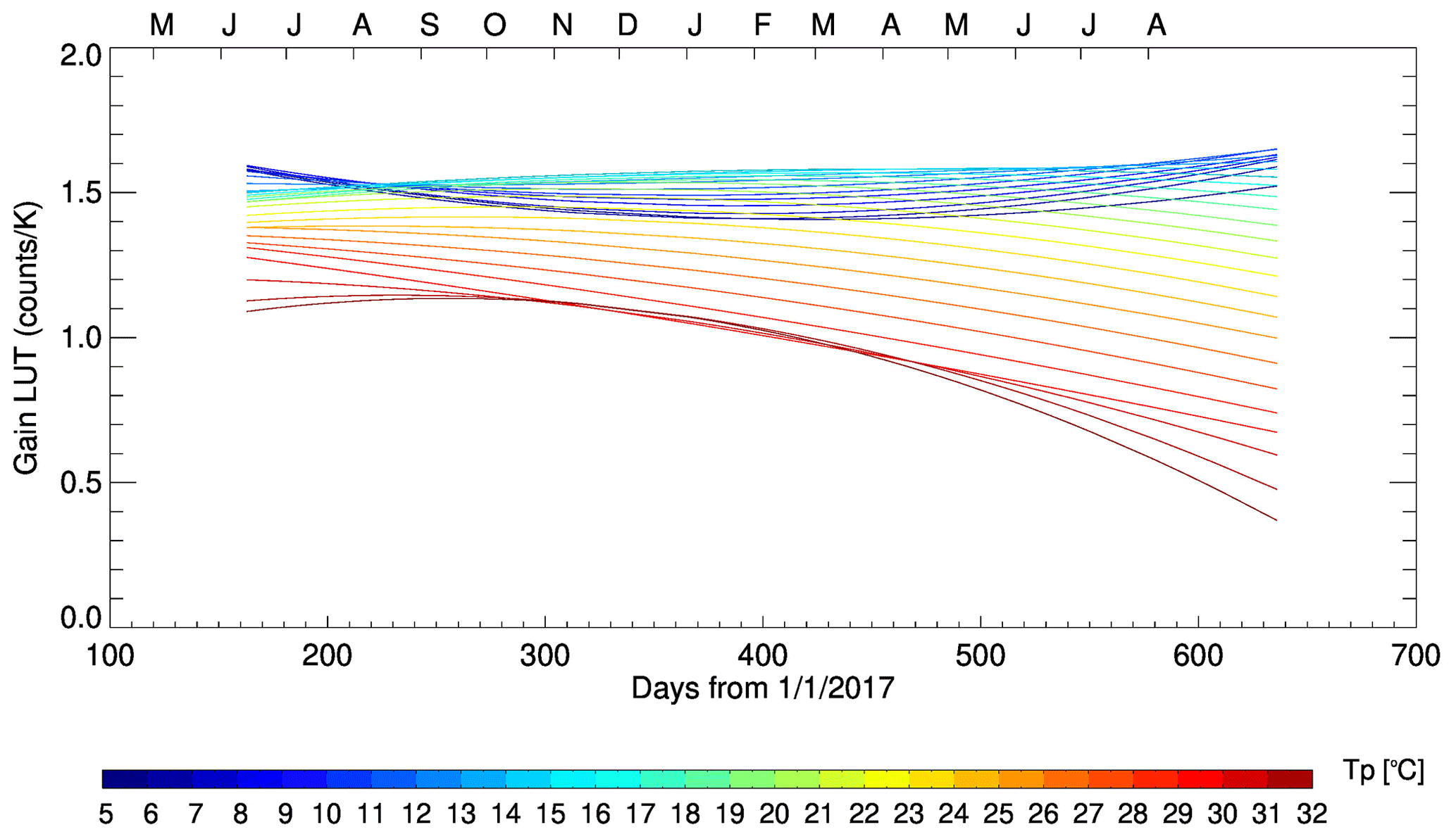
Gain was computed on a daily basis from the ratio of Ce and Tccr as a function of Tp4. Every day we can compute the two-dimensional statistics from the global samples and identify the most probable Tp4–G relationship. A second-order polynomial fitting was then applied to parameterize this relationship so to construct the final lookup table (LUT) as shown in Fig. 6. The daily variation of G is plotted in Fig. 5, separately for day and night. We can see that although the night yield of high-quality observations is fewer than that during the daytime because IceCube was turned off during most of the night to save power, the magnitude of gain and its degradation over time are almost identical. Therefore, we do not separate day and night in the final construction of the LUT. Yet small variations in the gain can be visually identified from Fig. 5, which is nevertheless omitted with using the LUT in Fig. 6. But in rare situations when the daily gain dropped dramatically (e.g., the outlier at ∼ day 270 in Fig. 5), data collected for the abnormal day were excluded completely. It is worth mentioning the history of the gain. It was measured at 2.37 count K−1 at 20 ∘C during the instrument thermal vacuum test (TVAC). However, it dropped to 1.1 count K−1 at 20 ∘C after the integration and testing (I&T) phase, which was suspected to be caused by debris falling into the unprotected receiver's feedhorn during the I&T phase. Nevertheless, the in-flight gain at 20 ∘C (black circles in Fig. 5) fortunately never dropped to below 1.3 count K−1. Ce is converted to TB using the gain LUT shown in Fig. 6. Furthermore, TB values are flagged as “poor quality” when the gain is smaller than 0.9.
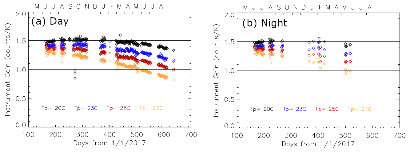
Figure 5Time series of daily gain for (a) daytime and (b) nighttime when the Tp4 value equals to 20 ∘C (black), 23 ∘C (blue), 25 ∘C (red) and 27 ∘C (orange). The gain declines consistently with increasing instrument temperature.
As the final step, TB is computed from Eq. (1). Note that we can also estimate the uncertainty of TB at the same time, which is 2–4 K for most orbits. Details of the TB uncertainty estimation can be found in Appendix D.
3.1 Comparison against model simulations
To evaluate the quality of the IceCube Level 1 TB, we will first compare the general statistics of TB against RTM simulations. The RTM employed here is the ARTS model. This model is chosen not only because it is one of the very few RTMs that can conduct cloud simulations at 874–883 GHz but also because of its well-developed comprehensive ice scattering databases and absorption spectrum at sub-millimeter frequencies (Buehler et al., 2018). CloudSat ice water content (IWC) profiles together with ECMWF ERA-Interim atmospheric profiles in the deep tropics (15∘ S–15∘ N) during June, July and August 2017 are used as the input parameters for ARTS model simulations, because 883 GHz is the least impacted by surface emissivity contaminations in the humid tropics, and IceCube data quality was the best in these 3 months of flight. To limit the “beam-filling” effect, this comparison is only limited to IceCube observations within ±15∘ viewing angles.
CloudSat carries a spaceborne 94 GHz nadir-pointing Cloud Profiling Radar (CPR) orbiting on a sun-synchronized afternoon polar orbit. The synthetic 883 GHz TB is generated using the “dBZ-based” (decibel relative to Z) method described in detail in Ekelund et al. (2020). Briefly speaking, given a particle size distribution (PSD) and a particle shape model (PM), the radar backscattering cross section from ice and/or liquid can be computed and associated with CloudSat radar reflectivity. An onion-peeling method is then applied from the cloud top down layer by layer to account for the two-way radar attenuation in each layer by IWC or rain water content (RWC) as well as multiple scattering. The IWC and RWC grids are calculated iteratively downward to construct the final profile. Then the retrieved IWC and RWC vertical profiles as well as ECMWF ERA-Interim atmosphere gas and water vapor are supplied to the forward model ARTS to compute the synthesized 883 GHz TB using the IceCube channel specification. Through this dBZ-based way, the consistency is kept for microphysics assumptions for hydrometeors between the CloudSat radar and IceCube radiometer.
Two particle PSDs, namely MH97 (McFarquhar and Heymsfield, 1997) and F07T (Field et al., 2007; tropics), are considered. MH97 has been used widely in the sub-limb and sub-millimeter community (e.g., Wu et al., 2006; Eriksson et al., 2007). In contrast to many other PSDs, MH97 uses the volume-equivalent (or mass-equivalent) diameter for the size (Dme) rather than the optically defined effective diameter (De), so the PSD-integrated mass is not dependent on density and is hence mass conserved with respect to different PMs. F07 is a single-moment PSD based on in situ data collected from multiple campaigns and has different settings for tropics (F07T) and mid-latitudes (F07M). Similar to the gamma-size PSD, it is not mass conserved. F07 has been used widely in the passive-microwave community (e.g., Kulie et al., 2010; Geer and Baordo, 2014) and is believed to have a better representation of precipitation-sized frozen particles, while MH97 is believed to represent anvil or cirrus ice better (a good comparison is given in Fig. 2 of Ekelund et al., 2020). Eight particle shape models are tested for each PSD assumption, as listed in the legend of Fig. 7. Random orientation is assumed for all simulations. More descriptions of model setups, including sensitivity to PSD and PM assumptions, can be found in Ekelund et al. (2020).
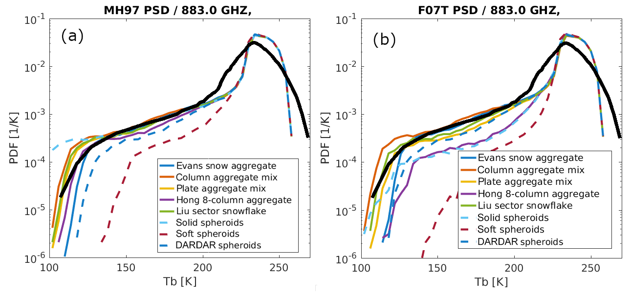
Figure 7PDF comparison of the IceCube TB (bold black line) against various ARTS model simulations using 3 months of tropical CloudSat observations and different ice shape assumptions and two particle size distribution assumptions: (a) MH97 PSD and (b) F07 PSD. Only IceCube observations within a ±15∘ viewing angle, at 15∘ S–15∘ N and during June–July–August 2017 are considered.
Based on the PDF comparison of simulated and observed TB shown in Fig. 7, we can clearly see that model simulations capture well the peak of the IceCube-observed radiances, although the clear-sky variation (roughly for TB>220 K) is significantly smaller than that observed. If Gaussian noise with width of 7 K is added to the ARTS simulation, it can greatly mimic the IceCube statistics (not shown); we thus speculate that the warm-end discrepancy is likely induced by the nosier IceCube data. This Gaussian shape of random noise mainly originates from three components: error induced by gain uncertainty, space count prediction and geolocation registration. The former two factors are explained in more detail in Appendix D, which is 2–4 K. The third factor's contribution is therefore estimated to be ∼3 K. Nevertheless, we cannot completely exclude other factors; e.g., the water continuum might be slightly overrepresented in the model. At the cold end however, model–observation discrepancies reveal interesting microphysical information. Firstly, none of the spheroid PM assumptions could make TBs cold enough that IceCube observes (except a solid spheroid with an MH97 assumption), indicating that current sphere or spheroid assumptions in many retrieval algorithms and model microphysical schemes are probably wrong or at least not sufficient to capture the observed cloud ice variabilities and radiative properties. Furthermore, even for non-spheroid particles, the differences among produced PDFs are discernible as well. For example, the “Hong eight-column aggregate” (purple solid) seems to capture the observed statistics with the MH97 assumption well but apparently produces a TB that is too warm with the F07T assumption. This particle shape is very similar to the PM assumption used in the current MODIS cloud retrieval algorithms (six-column aggregate; Platnick et al., 2017), where a gamma-size distribution is assumed. Recall that the sub-millimeter spectrum has a similar penetration depth as the passive visible spectrum (Fig. 1b). Such an inconsistency could therefore only be explained by the inconsistent PSD assumptions or the fact that IceCube and the MODIS visible band are observing different parts of the ice particle size spectrum. Another discernible discrepancy is from the simulation using DARDAR microphysics (blue dashed line in Fig. 7). DARDAR is a joint CloudSat radar and CALIPSO lidar IWC retrieval product which is believed to provide the best global knowledge about IWC vertical structures by far. However, with the DARDAR spheroid assumption, neither of the PSDs could reproduce IceCube ice observations in the upper troposphere. This strongly indicates that the “one-size-fits-all” approach does not work for all cloud ice particles. Aggregates and an aggregate mix seem to overall produce the best match to the IceCube observations. The spread of the simulated PDF lines occurs at a warm TB (∼220 K), which indicates that the sub-millimeter channel is more sensitive to a particular shape than MW channels (e.g., similar simulations carried for 190 GHz in Ekelund et al., 2020).
To summarize this section, the comparison between the IceCube TB distribution and a variety of ARTS model simulations demonstrates the good quality of IceCube data, especially for the cold ice cloud. The difference on the warm-end widths indicates that IceCube data probably contain ∼7 K of random noise (see Appendix E for IceCube instrument noise estimation using ARTS simulations). On the other hand, the spread of the simulations covers the IceCube measurements fairly well, reflecting the model's capability at simulating cloud ice scattering at the sub-millimeter range. This model serves as the core RTM for the upcoming Ice Cloud Imager (ICI) mission with all channels at the sub-millimeter range. Therefore, IceCube Level 1 data (Gong and Wu, 2021) provide a valuable asset for model validation and testing.
3.2 Comparison against other observations
In this section, IceCube TB will be compared against two other independent spaceborne observations at collocated footprints to validate the quality of IceCube cloud radiance measurements. These comparisons will be further compared with previous airborne campaign observations to evaluate the consistency and accuracy of IceCube Level 1 data.
The two independent spaceborne observations are the CloudSat 2B-CWC-RO (radar-only cloud water content) IWC retrieval product (version 05) and CALIPSO Imaging Infrared Radiometer (IIR) cloud product (version 4.20). We chose the CloudSat 2B-CWC-RO product instead of the DARDAR product that was used in the previous section simply because DARDAR data were not available for the IceCube flight period at the time when this part of the research was conducted. IIR was chosen because of two considerations. First, it is a passive IR radiometer, so we can scrutinize the sensitivity window overlaps between sub-millimeter and IR techniques on the IWP spectrum. Secondly, IIR has a 1 km2 footprint size and a 64 km×64 km swath, and it is geolocated with the CALIOP (Cloud-Aerosol Lidar with Orthogonal Polarization) lidar. It has three medium-IR broadband channels centered at 8.65, 10.6 and 12.05 µm. IIR's cloud product was retrieved against collocated CALIOP lidar measurements and then extended to the entire swath. Therefore, it has the advantage of high spatial resolution, high accuracy and a wider swath than lidar (hence more collocation samples with IceCube). Details of IIR cloud product retrieval algorithms and evaluation can be found in Garnier et al. (2013, 2020).
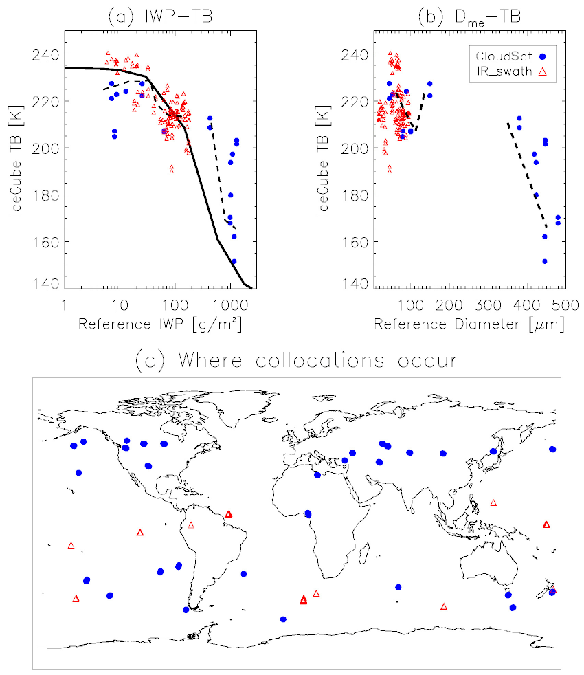
Figure 8IceCube TB generally shows good correlations with CloudSat (filled blue circle) and CALIPSO-IIR-retrieved (open red triangle) IWP (a) and Dme (b). Places for the collocations are marked in (c) with corresponding symbols. ARTS-simulated TB–IWP relationship (the solid black line from Fig. 1a) is overlaid in panel (a). Dashed lines connect the mean of every IWP or De bin, where the bin size is determined on a log scale for IWP and linear scale for De. Note that CloudSat IWP is calculated from the 2B-CWC-RO V05 IWC product and integrated between 7–15 km.
Collocated observations between CloudSat-, IIR- and IceCube TB observations within a ±30∘ viewing angle are identified globally and mapped on Fig. 8c as blue filled circles and red triangles, respectively. The collocation criteria are defined as the time difference within 10 min and distance within 30 km. We can see collocation samples are too limited to make robust statistics. However, they are enough to put together a steep and near-linear TB–IWP relationship that agrees with ARTS model simulation in a broad sense (Fig. 8a, model simulation is taken from the one on Fig. 1a), although model simulation seems to overestimate the TB depression at a larger IWP. Note that the partially column-integrated IWC profile in the middle-to-upper troposphere (7–15 km), or pIWP, computed from CloudSat retrievals has been presented and compared here to account for the maximum penetration depth of IceCube observations in the mid-latitudes according to a mid-latitude case simulation in Gruntzun et al. (2018). We tried different bottom heights for the pIWP integration and found that the slope barely changed. We can also see from the limited collocated samples that IceCube only starts to show sensitivity to IWP when it exceeds 40 g m−2, which agrees beautifully with the RTM simulation even though this simulation has quite some oversimplified settings.
Moreover, IceCube TB is found to show some sensitivity to the equivalent sphere diameter De in the 50–100 µm range before the slope becomes chaotic (Fig. 8b). We will revisit this point in the comparison with a field campaign below.
So far the only other two passive sensors that carry a 874–883 GHz channel are ESA's airborne International SubMillimeter Airborne Radiometer (ISMAR) and NASA's airborne Compact Scanning Submillimeter-wave Imaging Radiometer (CoSSIR). ISMAR only added the 874 GHz channel in recent flights, so data are not publicly available at this moment (Hammar et al., 2018; Fox, 2020). CoSSIR channel frequencies range from 183±1, ±3, ±7 GHz (water vapor profiling), 220, 380±1, ±2, ±3, ±6 GHz (temperature profiling) and 640 GHz vertically polarized and horizontally polarized pairs to 874 GHz. Designed with both conical and cross-track scan patterns, CoSSIR was onboard the NASA ER-2 aircraft and deployed to the TC4 (Tropical Composition, Cloud and Climate Coupling) campaign together with the 94 GHz Cloud Radar System (CRS) (Zhang and Monosmith, 2008). Comparison between CoSSIR 874 GHz and CRS retrievals is equivalent to comparisons between IceCube and CloudSat except that the in-flight comparison should yield a much cleaner and more robust relationship because of the perfect collocation, lower noise level and fortune to sample deep convective systems during the TC4 campaign. Evans et al. (2012) and Davis et al. (2010) described detailed retrieval procedures for Dme and IWC from CoSSIR. Dme is the mass-weighted equivalent sphere diameter, defined as
where N is the number density. Evans et al. (2012) has proven that a dedicated suite of MW and sub-millimeter cloud radiometers such as CoSSIR can achieve the vertical profiling of cloud ice. Gong and Wu (2017) demonstrated the usefulness of polarized 640 GHz radiance measurement on inferring ice crystal shape and orientation.
Collocated CoSSIR 874 GHz TB–CRS IWP and Dme are scattered in Fig. 9. To make a fair comparison, only cross-track scan samples with viewing angles <30∘ are used. Also, again the partial column integration is used for IWP and Dme calculation but for 9 km above instead of 7 km above for CloudSat pIWP integration. This consideration is to account for the tropopause height difference between the mid-latitudes and deep tropics because almost all CloudSat–IceCube collocations happen at mid-latitudes, while the TC4 campaign flew in the deep tropics. Comparisons from IceCube–CloudSat and IceCube–IIR are overlaid as blue filled circles, and the difference between physical meanings of Dme and De is ignored here. To account for gas absorption between the flight altitude and satellite altitude, a 10 K warm offset is added to the spaceborne comparison data. From visual inspection we can tell the TB–IWP and TB–Dme relationships are robust and consistent with those spaceborne relationships. The scattered spaceborne observations at ∼1000 g m−2 and 400–500 µm are from one collocation overpass over the central US. While it is reasonable to argue that these may be outliers or caused by imperfect collocations, their spread and mean values indicate the upper boundary of 874 GHz sensitivity thresholds, as also suggested by the flattening end to the right of Fig. 9 from the campaign data.
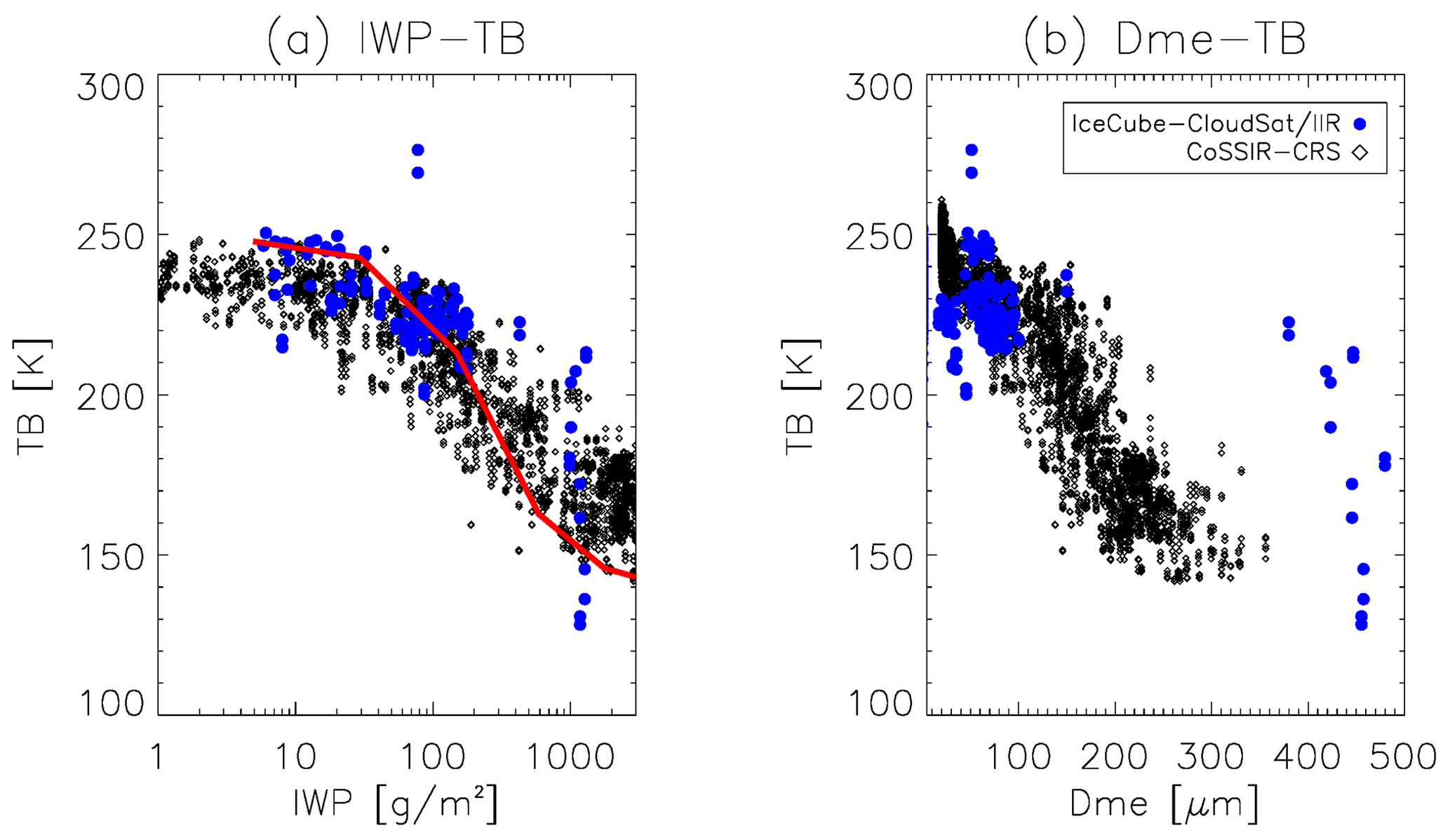
Figure 9(a) IWP–TB and (b) Dme–TB relationship derived from collocated CoSSIR–CRS measurements (black dots) during the TC4 campaign. Note that IWP here is the partial column integration from 9 km above. IceCube–CloudSat–IIR data from Fig. 8 are overlaid as blue dots with a warm offset of 10 K added. ARTS simulation (red curve) is added as the reference.
In summary, TB–IWP and TB–De relationships observed by collocated IceCube and other independent spaceborne observations show impressively good agreement with RTM prediction as well as airborne observations. Based on these two sets of comparisons, we can conclude that IceCube observations can indeed fill in the sensitivity gap between passive IR and MW sensors for IWP and ice particle size. CoSSIR is anticipated to be deployed again in the near future for the IMPACTS (Investigation of Microphysics and Precipitation for Atlantic Coast-Threatening Snowstorms) campaign, where more 874 GHz measurements are going to be collected from mid-latitude winter frontal systems. IceCube data (Gong and Wu, 2021) can be used as observational references for future RTM simulations or feasibility studies for developing new sub-millimeter instruments (e.g., CoSSIR and ICI).
IceCube provides the first-ever global ice cloud observation at 874–883 GHz. Although IceCube was not designed as a science mission, it is still worthwhile exploring and discussing the scientific value of this dataset (Gong and Wu, 2021). We do not intend to provide the Level 2 retrievals at this moment mainly due to two considerations. Firstly, the geolocation registration has ∼14 km uncertainty as aforementioned. As clouds can often be very inhomogeneous, pixel-by-pixel retrieval might yield poor quality, especially at large viewing angles. Despite this, we will show in the last example that IceCube data can be used for weather-scale studies as well. Secondly, with only one single-frequency channel, the retrieval cannot avoid large uncertainties induced by microphysics assumptions. Even it is backed up by sophisticated RTM simulations, one can clearly see from Fig. 7 how different microphysics assumptions can make huge differences in the simulated TB and therefore impact the retrieved IWP. Nevertheless, IceCube data (Gong and Wu, 2021) are suitable for climatology studies. The IceCube-observed cloud ice distribution and diurnal variation can help reveal the physical processes that were missing in the IR and MW pictures.
To avoid arbitrarily setting too many assumptions before using an RTM (e.g., ARTS) for retrieval, we applied the empirical relationships of TB–pIWP and TB–Dme derived from the airborne campaign CoSSIR–CRS collocation statistics shown in Fig. 9. A 10 K gas absorption offset is added to IceCube TB before the conversion. Apparently a positive value of IWP or Dme should not be assigned for every TB observation. Accounting for the sensitivity range and general statistics, a commonly used cloud-screen method, called the iterative 3σ method, is used. This method and the empirical retrieval approach has been used previously in Gong and Wu (2014) and Wu et al. (2014). A 10-loop iteration is carried out to screen out the clear-sky TB. In each iteration, the standard deviation σ and the corresponding peak value TBpeak are calculated, and then any TB values below the TBpeak−2σ threshold are excluded from the next iteration step. After several iterations, the contribution from the long left tail of the TB's PDF to the skewness can be removed, and the Gaussian spread of the clear-sky variability can be relatively well captured. We then apply TBpeak−3σ from the last iteration step as the threshold to separate clear-sky and cloudy-sky scenes. Only pixels with are used for the “retrieval”. This procedure has been carried out monthly for every 5∘ latitude band and only for observations at viewing angles <30∘.
Figure 10 shows the geographic distribution of the mean IWP, cloud occurrence frequency (OF) and mean Dme for June–July–August 2017 and 2018 (left) and January–February 2018 (right). December 2017 was not included because of too few data samples collected during that month. Note that by saying IWP, it is actually the partially column-integrated pIWP from about 9 km above in the tropics and 7 km above in the mid-latitudes based on the empirical relationships. As expected, large IWP, OF and Dme measurements are identified in the tropical deep convective regions. The geographic distributions of IceCube IWP agree well with Aura Microwave Limb Sounder (MLS) 640 GHz pIWP retrieved above 10 km (Wang et al., 2021), Odin SMR (501 and 554 GHz; Submillimeter wave Radiometer) and SMILES (624–650 GHz; Superconducting Submillimeter-Wave Limb-Emission Sounder) pIWP retrieved above 260 hPa (Eriksson et al., 2014). Overall the magnitude of IceCube IWP is slightly larger than the above three other passive satellite measurements but within good agreement with CloudSat pIWP above 260 hPa (Eriksson et al., 2014). This is more or less expected because we used the empirical relationship, while Odin SMR and SMILES pIWP retrievals are based on RTM simulations, while Aura MLS 640 GHz retrieval is based on the empirical relationship against the CALIPSO lidar. OF derived from IceCube data ranges between 15 %–30 % in the tropical deep convective regions. Comparing to MODIS IR band ice cloud coverage retrieved at 40 %–80 % in the same regions which is more widely spread (Wang et al., 2016) and to CloudSat-observed deep convective clouds occurring at a frequency of 5 %–20 % in the deep tropics and more narrowly defined (Sassen et al., 2009), we can thus reconfirm that an observed sub-millimeter cloud is in the middle of the developing processes of deep convective systems between deep convective clouds and IR-observed cirrus and anvils when they spread out, as well as in the middle of the decaying processes when the anvil and cirrus clouds settle down. Mean Dme however, starts to lose its geographic differentiation in these regions, indicating the sensitivity threshold in deep convective regions. Other than tropical deep convective regions that migrate with the season shift, coherent enhancements of the three parameters are also found at the Southern Ocean storm track and cold-air outbreak regions in austral winter and North Atlantic storm track regions in boreal winter.
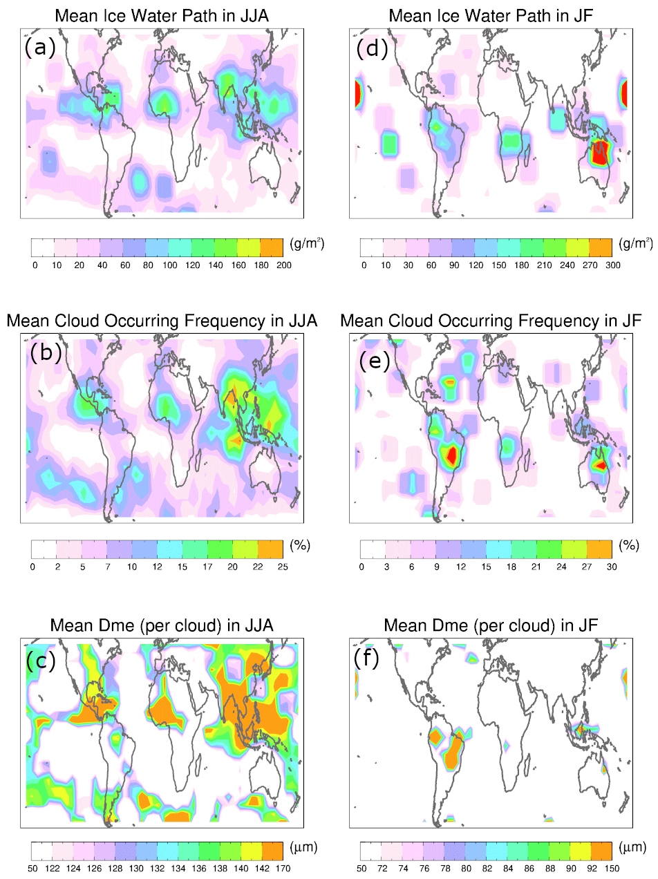
Figure 10Global distribution (55∘ S–55∘ N) of IceCube pIWP (a, d), cloud occurrence frequency (b, e) and cloud mean Dme (c, f) for June–July–August 2017 and 2018 (a, b, c) and January–February 2018 (d, e, f). Grid box size is 5∘ latitude × 7.5∘ longitude.
As we argued about the importance and unique merit of sub-millimeter techniques, it is more straightforward to compare the diurnal cycle from sub-millimeter observations with surface precipitation to identify some plausible coupling processes between the cloud and precipitation. Figure 11 overlaps the diurnal cycle of IceCube cloud IWP with that of the surface precipitation rate (PRS) retrieved by the Global Precipitation Mission Dual Precipitation Radar (GPM-DPR) in the deep tropics (20∘ S–20∘ N) for ocean and land conditions, separately. Over tropical land, we can see that the IceCube cloud diurnal cycle lags the minima and maxima of surface precipitation by ∼3–5 h. Early-evening heavy precipitation at around 17:00 LST (local solar time) is well-known as a result of the development of tropical mesoscale convective systems (MCSs) (Nesbitt and Zipser, 2003). While deep convective systems downpour, its upper level cloud continues to develop and spread out. IceCube cloud IWP peak timing (22:00 LST) strongly suggests they are likely anvils or thick cirrus. As land convection calms down and eventually dissipates and surface precipitation reaches minimum at ∼ 10:00 LST, the upper-level cloud does not completely dissipate until noon. So from the diurnal cycles of precipitation and clouds over land, we may conclude that these IceCube-observed clouds are likely dominated by those deep convective clouds and cloud systems.
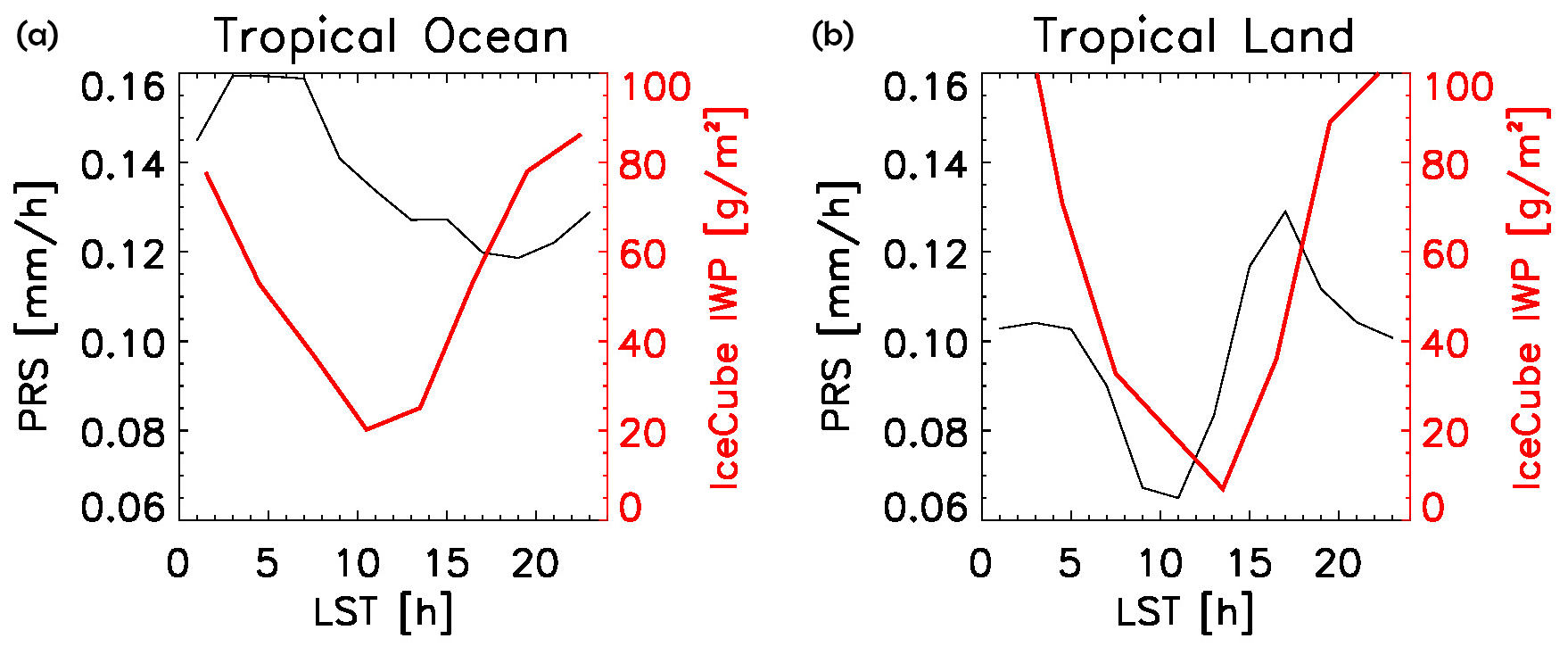
Figure 11Diurnal cycle for IceCube IWP (red) and surface precipitation rate (PRS) derived from GPM-DPR radar (black) over tropical ocean (a) and land (b) with respect to local solar time (LST). Only IceCube data within a ±30∘ viewing angle are used for generating these statistics, and the tropics are bounded by 20∘ S and 20∘ N. Time interval is every 3 h, and IceCube does not have samples between 22:00 to 01:00 LST.
However, the diurnal cycle of precipitation and IceCube cloud over tropical ocean tell a different story. Firstly, the magnitude of the diurnal cycle of oceanic precipitation is significantly smaller than that over tropical land, although the mean is larger, which has been reported previously in literature. The overall precipitation peak at 05:00 LST is believed to be a mixed signature among isolated convection, shallow convection and MCSs (Nesbitt and Zipser, 2003). However, an IceCube-observed ice cloud leads the development of surface precipitation by about 5 h, as does the trough (i.e., dissipation phase). This hints that stratiform precipitation forming from anvils rather than bottom-up convective downpours is likely the dominant physical process in determining the diurnal cycle of the tropical oceanic precipitation. This speculation explains the opposite phase lag between the diurnal cycle of IWP and surface precipitation over tropical ocean versus land. It is also supported by the longer time delay over ocean (∼5 h) than over land (∼3 h), as it takes a longer timescale for the stratiform precipitation particle to form from the anvils and to fall down to the ground. Using Tropical Rainfall Measurement Mission (TRMM) products, Yang and Smith (2008) found that stratiform precipitation dominated the tropical oceanic precipitation throughout the day, with more contributions from local afternoon to midnight. This partially supports our hypothesis. Nevertheless, we could only complete the picture of the convection-cloud–precipitation process by wisely using a combination of satellite observations that detect different components of this entire process.
There are some caveats to this diurnal comparison though. IceCube does not collect enough cloudy-sky samples between 22:00 and 01:00 LST in the tropics, so the diurnal cycle is not complete. Due to the same reason, we cannot further scrutinize different regions (e.g., maritime continent), so different mechanisms are unavoidably mixed together. Moreover, the IceCube diurnal cycle over tropical land is similar to that derived from SMILES, but its diurnal cycle over the tropical ocean is too strong compared to that of SMILES (Millan et al., 2013; Eriksson et al., 2014). The discrepancy between the two passive sub-millimeter missions could not be understood without further sub-millimeter missions that scan Earth at different local times. Multiple channels will greatly improve the retrieval quality and increase the retrievable microphysical parameters (Eriksson et al., 2020).
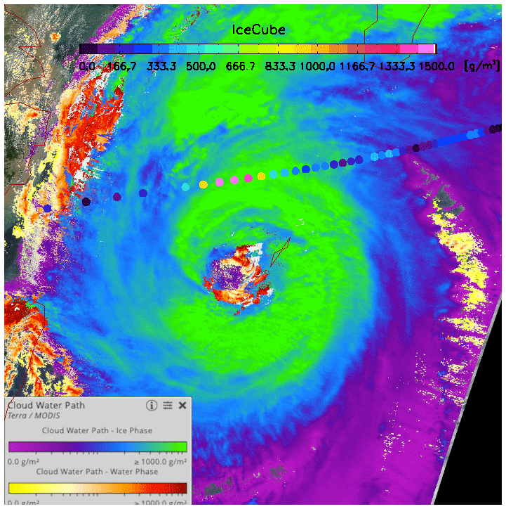
Figure 12IWP retrievals of Typhoon Trami on 29 September 2018 from an overpass of IceCube (color bar on the top) and Terra–MODIS (color bar on the bottom left corner). Their time difference is about 1.5 h. MODIS retrieval image is from https://worldview.earthdata.nasa.gov (last access: 11 November 2021). We acknowledge the use of imagery from the NASA Worldview application (https://worldview.earthdata.nasa.gov, last access: 11 November 2021), part of the NASA Earth Observing System Data and Information System (EOSDIS).
In the last example to demonstrate IceCube data's scientific merit, we show a case study of Typhoon Trami (Fig. 12). IceCube overpassed this typhoon on 29 September 2018 at an orbital altitude of ∼250 km 4 d before it re-entered Earth's atmosphere. However, it was still capable to yield a set of scientifically valuable observations in terms of both the retrieved IWP value range compared with Terra MODIS retrievals, as well as the geolocations. Although there is a ∼1.5 h time difference between the Terra MODIS and IceCube measurements, both observations exhibit good agreements with each other: large IWP values (>1000 g m−2) for the northern arm and medium IWP values (200–500 g m−2) for the outer bands. IceCube data show a sharp gradient of retrieved IWP from left to right across the northern arm, while the MODIS visible band apparently saturated and cannot tell more detailed structures within the band.
Data processing codes are available upon request.
IceCube Level 1 data are available in NASA's Open Data Portals at Gong and Wu (2021) (https://doi.org/10.25966/3d2p-f515). They are also available to the public on the main IceCube website at https://earth.gsfc.nasa.gov/climate/missions/icecube/ (last access: 11 November 2021). A list with variable names and their meanings can be found in Appendix F.
IceCube carries the first-ever spaceborne 874–883 GHz radiometer, which kept on acquiring Earth's ice cloud measurements for more than 15 months. In this paper, we discussed the motivation and algorithms to obtain IceCube Level 1 radiance data (Gong and Wu, 2021). The detailed procedures for data processing have been documented in Sect. 2. The main steps include space count prediction and calibration, viewing angle determination and geolocation registration, and gain model construction. The processed IceCube radiance data are then compared with RTM-simulated clear-sky radiances, collocated active and passive satellite observations, and airborne campaign data to validate their quality. Overall IceCube Level 1 data are found to be of good quality at near-nadir viewing angles. Data quality in general decreases in 2018 compared with 2017 because of instrument degradation. The estimated uncertainty of IceCube radiance data is ∼7 K.
Scientific values of IceCube data are discussed with three examples presented. The first is the global 883 GHz cloud ice map. The agreement and disagreement with what have been found from other passive and active spaceborne measurements demonstrate unique assets of this dataset in filling the missing piece of the entire coupled cloud–precipitation process. Then we show the diurnal cycle to further demonstrate this point. A typhoon case is given at last to showcase that IceCube data are unique and important not only for understanding the climatologies but also valuable for weather scale studies.
A few sub-millimeter sensors will hopefully be launched to space in the upcoming years. Together with their airborne and ground variants as well as their predecessors such like IceCube, we will gain more comprehensive understanding of this band and explore more capabilities from this band for better monitoring and predicting Earth's weather and climate.
As CloudSat, CALIPSO and AIRS are the spaceborne radar, lidar and passive infrared sensors flying on the A-train constellation, only 1 month of tropical collocation statistics (January 2009, 30∘ S–30∘ N) is robust enough. The collocation criteria is defined such that the spatial difference should be less than 5 km, and temporal difference should be less than 1 min. AIRS water vapor channel no. 1247 (wavenumber=1128.57 cm−1) is employed here. AIRS Tcir is computed by subtracting Level 2 cloud-cleared radiance (Tccr, version 6) from Level 1B brightness temperature TB (version 5). The CloudSat–CALIPSO joint IWP retrieval product 2C-ICE (version 4) is used as the truth showing on the horizontal axis. In the case that multiple CloudSat–CALIPSO footprints collocated with one AIRS footprint, the IWP values retrieved from the former are averaged first before constructing the two-dimensional PDF. The blue solid line connects the peaks of the AIRS–CloudSat–CALIPSO two-dimensional PDF.
To construct MHS's Tcir–IWP relationship, collocated tropical near-nadir samples from multiple months are used to compile the statistics. Details about collocation criteria, the near-nadir definition, etc. can be found in Gong and Wu (2014). Different from the above blue line, the black dashed line is created from an ARTS model simulation at 190 GHz by inserting a Gaussian shape of an ice cloud layer between 150 and 600 hPa with a peak at 400 hPa. One can see that the RTM simulation, even when using an idealized cloud layer, can accurately mimic the observed Tcir–IWP relationship, indicating that MW channels are more sensitive to the total mass than to the vertical structure.
The black solid line is based on another ARTS model simulation at 874 GHz with the same ice cloud configuration. For both the simulations at 190 and 874 GHz, Tcir is derived by subtracting the simulated clear-sky radiance (i.e., setting IWC=0 in the entire column), so any surface contribution is excluded using this strategy.
Figures 2 and 3 only give an example of good measurements. In the later time of the IceCube mission, various experiments were tested to gain knowledge of instrument behavior under different scenarios. Figure B1 and B2 here gave an example of a poor-quality orbit. IceCube was kept on for several orbits actually, but the instrument temperature was kept under 35 ∘C. As a result, one can clearly see the oscillation in the later part of this orbit, and the Ce–Csp contrast declines over time due to the relatively high temperature (Fig. B1a). In Fig. B1d, it is also clear that the periodic low-frequency oscillation of Csp against Tp3 and Tp4 also changed after Tp4 hit the temperature cap and IceCube was cooled down and then heated up again. As a result, Fig. B1c and d failed to capture the slowly varying oscillations of Csp. Therefore, we need to further apply a fitting to Csp (green line in Fig. B2), and the final Ce now remains largely stable among different spins (red dots of Fig. B2, shifted upward by 200 counts). Some spins that have too low of a Ce–Csp contrast (e.g., the five spins between s and s) or too slow of a spin velocity (e.g., the last four spins) are excluded.
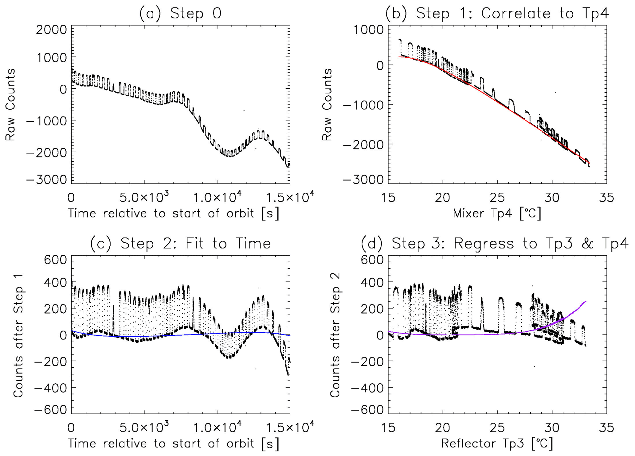
Figure B1Same with Fig. 2, except this is an example showing a bad-quality orbit. This orbit is the second orbit of IceCube on 2 April 2018.

Figure B2Same with Fig. 3, except this is the final step for the case in Fig. B1. The final polynomial fitting to the space-view counts only is a very necessary step to capture the slowly varying component of the time series, which was failed to be captured in the step 3 based on Fig. B1c using all-sky counts. Please note that the date format in this figure is year month day.
Empirical relationships have been used in steps 1–4 to account for the majority of Csp variations even for irregular orbits like the one shown in Fig. B2. Therefore, the residual between observed Csp and predicted ones remain stable with a standard deviation of ∼4 K (black crosses in Fig. 4). During these procedures, instrument parameters such as spin rate (spinx, spiny and spinz), measured magnet field (Magx, Magy and Magz) were not used. They were believed to not affect Csp in the pre-launch tests. As such, the ML/AI model is only included in this Appendix for the purpose of testing the robustness of this approach in reducing any generic instrument noise for IceCube and future CubeSat type missions or constellations that are less well calibrated due to the low cost cap. In the final product, we provide both the TB before and after this ML/AI step for the user to select.
Only the random forest model was tested for this work. As we can see from the poor-quality orbit case in Fig. B1b and d, Csp shows a hint of slight elevation after IceCube has been switched on for a long time given the same Tp3 and Tp4. Therefore, relative change in time and temperature with respect to the switch-on parameters for each orbit are also factored in as DT1, DT2, DT3, DT4 and DTime. The Julian day counted from 1 January 2017 is marked as “time”. As there is no need or intention to “predict for the future” but rather to capture the fast-varying and slow-varying components of the Csp residual, we split the total samples randomly so to assign 70 % for training and the remaining 30 % for testing and validation. This is different from a traditional ML/AI model performance check and admittedly makes some caveats to the argument. Only 30 % of the testing sample statistics are shown in Fig. C1.
As one can see from the heatmap in Fig. C1a, the majority of the predicted residual is centered around 0 K, meaning that the trained model can largely capture the residual variations most of the time (recall that “residual” is defined as the discrepancies between the predicted and the observed Csp values). It also indicates that there is no associated bias to skew the statistics. The standard deviation of the predicted residual σsp is ∼2 K as opposed to ∼4 K before the ML/AI treatment, which is a direct reflection of the strength of this ML/AI approach in capturing the sophisticated, “white-noise-like” features of the residuals. In the meantime, large residual values up to ±10 K, showcased along the 1:1 line in the heatmap, can be produced as well. These values mainly occur at the start and end of the Earth-view leg with big slant viewing angles.
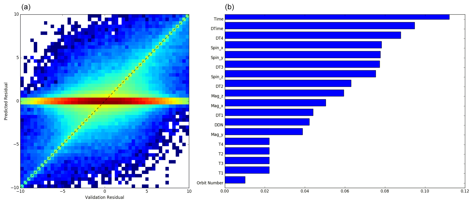
Figure C1(a) Heatmap of the predicted Csp residuals (vertical axis) against the observed ones (horizontal axis), colored in log-scale. (b) Rank of importance of different parameters. Spin(Mag)_x, _y and _z correspond to the spin rate (magnetic field) on the x, y and z axes, respectively; DDN stands for the day of the year, and please refer to text in Appendix C for the meaning of other variables.
The rank of importance among all variables can help further diagnose the sources of the residual time series. As expected, instrument degradation (i.e., time) and switch-on time duration affect the residual noise of Csp the most. In addition, the relative change of Tp4 and Tp3, indicated by DT4 and DT3, and the spin rate along three axes contribute about the same amount of importance to the final prediction.
The uncertainty (i.e., error bar) of derived TB can be calculated as follows. According to the definition of TB, ; therefore, the full derivative of TB, i.e., dTB, could be written as
The first term is uncertainty induced by gain estimation, and the second term is induced by the space count prediction. ΔC is calculated for each orbit as shown in Fig. 4, which should be ∼4 K (∼2 K) before (after) the ML/AI process. ΔG is computed from the standard deviation of PDFs of daily G, the value of which varies around 0.002–0.005 [counts K−1] for most days and occasionally reaches up to 0.02 [counts K−1]. dTB is thus calculated for each given Ce once TB is converted. This value is reported in the Level 1 data as well.
The ∼7 K instrument noise is estimated as shown in Fig. E1. With applying a 7 K random noise that follows the Gaussian distribution on the simulated TB, we can achieve an excellent agreement on spread of the warm side (red versus black lines), indicating that the warm-side discrepancy in Fig. 7 is indeed mainly induced by IceCube noise of ∼7 K. Note that this instrument noise includes the TB uncertainty quantified for each single observation using the method described in Appendix D. However, the total noise can only be quantified using the PDF method suggested here, and it is impossible to accurately capture this noise at a single footprint level.
Another interesting feature to notice is that the discrepancy between 220–235 K shown in Fig. 7 disappears if the model inputs are self-consistent in terms of particle shape and PSD when the retrieval algorithm is applied (i.e., DARDAR algorithm assumptions about microphysics are applied throughout the simulations in Fig. E1). We cannot reach a quick conclusion before rerunning a group of sensitivity tests. Unfortunately Fig. E1 was generated at the end of this project, and we do not have further resources to rerun sensitivity experiments like those in Fig. 7 again.
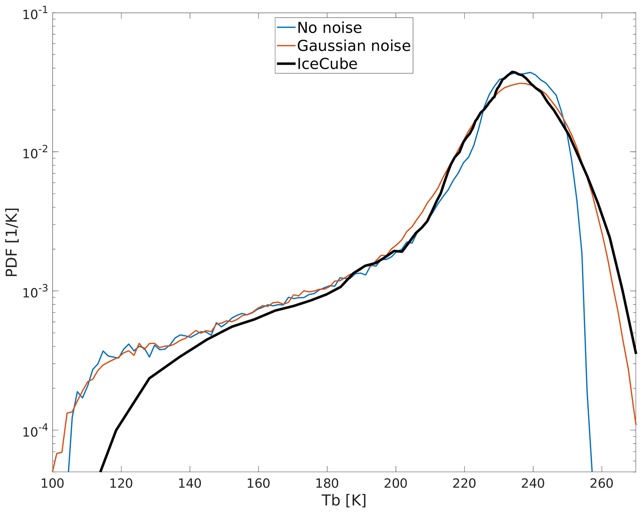
Figure E1PDF comparisons of IceCube TB (black) against ARTS model simulations using DARDAR retrieved IWC profiles as the input (blue) and the same simulation with 7 K Gaussian random noise applied (red). Only DARDAR profiles that are within the same area and time range of Fig. 7 are used and the simulation follows Ekelund et al. (2020).
IceCube Level 1 data (Gong and Wu, 2021) are stored in the HDF5 (Hierarchical Data Format) format. The data filename is IceCube.L1.YYYYMMDD.V01.h5, where YYYYMMDD indicates the year (four digits), month (two digits) and day (two digits).
The variable name list can be found below.
-
LAT – latitude; unit: [∘]
-
LNG – longitude; unit: [∘]
-
TB_MODEL – RTM-simulated clear-sky TB; unit: [K]
-
TB_OBS1 – observed TB; unit [K]
-
TB_OBS2 – observed TB with ML/AI-predicted residual subtracted (see Appendix C for details of this procedure); unit: [K]
-
TB_UNC1 – TB uncertainty; unit: [K]
-
TB_UNC2 – TB uncertainty after ML/AI treatment; unit: [K]
-
UTC – universal time; unit: [s]
-
VIEW_ANG – viewing angle from the nadir; unit: [∘]
-
DN_FLAG – day/night flag (0 for day, 1 for night); unitless
-
QC – quality control flag; unitless
-
0: good quality
-
1: geolocation quality is poor due to large viewing angle
-
2: quality is doubtable due to abnormal gain
-
3: quality is doubtable due to abnormal spin rate or instrument temperature
-
-
ORBIT_NUMBER – orbit number counted from the switch-on time to the switch-off time (every day reset to 0); unitless
DLW conceptualized the project and procedures for data calibration and processing. JG refined and improved the algorithm, conducted the data analysis, and wrote the manuscript. PE provided the ARTS model simulation. All authors were heavily involved in interpreting the results.
The authors declare that they have no conflict of interest.
Publisher’s note: Copernicus Publications remains neutral with regard to jurisdictional claims in published maps and institutional affiliations.
This work is supported by NASA (grant no. NNH19ZDA001N-RRNES). The authors are grateful to the entire IceCube team for the successful fabrication and launching of the IceCube instrument as well as industrious effort regarding the data collection. The NASA Earth Science Technology Office (ESTO) is acknowledged for the selection and support of the IceCube mission. Yuping Liu contributed to the early data processing and Tccr computation; this work was indispensable to the completion of the current paper. Helpful discussions with Stuart Fox, Anne Garnier, Inderpreet Kaur and Chenxi Wang are greatly appreciated.
This research has been supported by the National Aeronautics and Space Administration Goddard Space Flight Center (program ROSES-RRNES-2019).
This paper was edited by Ge Peng and reviewed by two anonymous referees.
Bosilovich, M. G., Robertson, F. R., Takacs, L., Molod, A., and Mocko, D.: Atmospheric water valance and variability in the MERRA-2 reanalysis, J. Climate, 30, 1177–1196, https://doi.org/10.1175/JCLI-D-16-0338.1, 2017. a, b
Buehler, S. A., Jiménez, C., Evans, K. F., Eriksson, P., Rydberg, B., Heymsfield, A. J., Stubenrauch, C. J., Lohmann, U., Emde, C., John, V. O., Sreerekha, T. R., and Davis, C. P.: A concept for a satellite mission to measure cloud ice water path, ice particle size, and cloud altitude, Q. J. Roy. Meteor. Soc., 133, 109–128, https://doi.org/10.1002/qj.143, 2007. a
Buehler, S. A., Mendrok, J., Eriksson, P., Perrin, A., Larsson, R., and Lemke, O.: ARTS, the Atmospheric Radiative Transfer Simulator – version 2.2, the planetary toolbox edition, Geosci. Model Dev., 11, 1537–1556, https://doi.org/10.5194/gmd-11-1537-2018, 2018. a, b
Davis, S., Hlavka, D., Jensen, E., Rosenlof, K., Yang, Q., Schmidt, S., Borrmann, S., Frey, W., Lawson, P., Voemel, H., and Bui, T. P.: In situ and lidar observations of tropopause subvisible cirrus clouds during TC4, J. Geophys. Res., 115, D00J17, https://doi.org/10.1029/2009JD013093, 2010. a
Duncan, D. I. and Eriksson, P.: An update on global atmospheric ice estimates from satellite observations and reanalyses, Atmos. Chem. Phys., 18, 11205–11219, https://doi.org/10.5194/acp-18-11205-2018, 2018. a
Ekelund, R., Eriksson, P., and Pfreundschuh, S.: Using passive and active observations at microwave and sub-millimetre wavelengths to constrain ice particle models, Atmos. Meas. Tech., 13, 501–520, https://doi.org/10.5194/amt-13-501-2020, 2020. a, b, c, d, e
Eliasson, S., Buehler, S. A., Milz, M., Eriksson, P., and John, V. O.: Assessing observed and modelled spatial distributions of ice water path using satellite data, Atmos. Chem. Phys., 11, 375–391, https://doi.org/10.5194/acp-11-375-2011, 2011. a, b, c, d
Eriksson, P., Ekström, M., Rydberg, B., and Murtagh, D. P.: First Odin sub-mm retrievals in the tropical upper troposphere: ice cloud properties, Atmos. Chem. Phys., 7, 471–483, https://doi.org/10.5194/acp-7-471-2007, 2007. a
Eriksson, P., Rydberg, B., Sagawa, H., Johnston, M. S., and Kasai, Y.: Overview and sample applications of SMILES and Odin-SMR retrievals of upper tropospheric humidity and cloud ice mass, Atmos. Chem. Phys., 14, 12613–12629, https://doi.org/10.5194/acp-14-12613-2014, 2014. a, b, c
Eriksson, P., Rydberg, B., Mattioli, V., Thoss, A., Accadia, C., Klein, U., and Buehler, S. A.: Towards an operational Ice Cloud Imager (ICI) retrieval product, Atmos. Meas. Tech., 13, 53–71, https://doi.org/10.5194/amt-13-53-2020, 2020. a
Evans, K. F., Wang, J. R., O'C Starr, D., Heymsfield, G., Li, L., Tian, L., Lawson, R. P., Heymsfield, A. J., and Bansemer, A.: Ice hydrometeor profile retrieval algorithm for high-frequency microwave radiometers: application to the CoSSIR instrument during TC4, Atmos. Meas. Tech., 5, 2277–2306, https://doi.org/10.5194/amt-5-2277-2012, 2012. a, b
Field, P. R., Heymsfield, A. J., and Bansemer, A.: Snow size distribution parameterization for midlatitude and tropical ice clouds, J. Atmos. Sci., 64, 4346–4365, https://doi.org/10.1175/2007JAS2344.1, 2007. a
Fox, S.: An evaluation of radiative transfer simulations of cloudy scenes from a numerical weather prediction model at sub-millimetre frequencies using airborne observations, Remote Sens., 12, 2758, https://doi.org/10.3390/rs12172758, 2020. a
Garnier, A., Pelon, J., Dubuisson, P., Yang, P., Faivre, M., Chomette, O., Pascal, N., Lucker, P., and Murray, T.: Retrieval of Cloud Properties Using CALIPSO Imaging Infrared Radiometer. Part II: Effective Diameter and Ice Water Path, J. Appl. Meteorol. Clim., 52, 2582–2599, https://doi.org/10.1175/JAMC-D-12-0328.1, 2013. a, b
Garnier, A., Pelon, J., Pascal, N., Vaughan, M. A., Dubuisson, P., Yang, P., and Mitchell, D. L.: Version 4 CALIPSO Imaging Infrared Radiometer ice and liquid water cloud microphysical properties – Part II: Results over oceans, Atmos. Meas. Tech., 14, 3277–3299, https://doi.org/10.5194/amt-14-3277-2021, 2020. a
Geer, A. J. and Baordo, F.: Improved scattering radiative transfer for frozen hydrometeors at microwave frequencies, Atmos. Meas. Tech., 7, 1839–1860, https://doi.org/10.5194/amt-7-1839-2014, 2014. a
Gong, J. and Wu, D. L.: CloudSat-constrained cloud ice water path and cloud top height retrievals from MHS 157 and 183.3 GHz radiances, Atmos. Meas. Tech., 7, 1873–1890, https://doi.org/10.5194/amt-7-1873-2014, 2014. a, b, c
Gong, J. and Wu, D. L.: Microphysical properties of frozen particles inferred from Global Precipitation Measurement (GPM) Microwave Imager (GMI) polarimetric measurements, Atmos. Chem. Phys., 17, 2741–2757, https://doi.org/10.5194/acp-17-2741-2017, 2017. a
Gong, J. and Wu, D. L.: IceCube Level 1 Radiance Data and Codes, NASA Open Data Repository [data set], https://doi.org/10.25966/3d2p-f515, 2021 (data available at: https://earth.gsfc.nasa.gov/climate/missions/icecube/, last access: 11 November 2021). a, b, c, d, e, f, g, h, i
Grützun, V., Buehler, S. A., Kluft, L., Mendrok, J., Brath, M., and Eriksson, P.: All-sky information content analysis for novel passive microwave instruments in the range from 23.8 to 874.4 GHz, Atmos. Meas. Tech., 11, 4217–4237, https://doi.org/10.5194/amt-11-4217-2018, 2018. a, b
Hammar, A., Sobis, P., Drakinskiy, V., Emrich, A., Wadefalk, N., Schleeh, J., and Stake, J.: Low noise 874 GHz receivers for the International Submillimetre Airborne Radiometer (ISMAR), Review of Scientifc Instruments, 89, 055104, https://doi.org/10.1063/1.5017583, 2018. a
Kulie, M. S., Bennartz, R., Greenwald, T. J., Chen, Y., and Weng, F.: Uncertainties in microwave properties of frozen precipitation: Implications for remote sensing and data assimilation, J. Atmos. Sci., 67, 3471–3487, https://doi.org/10.1175/2010JAS3520.1, 2010. a
Li, J.-L. F., Waliser, D. E., Stephens, G., and Lee, S. W.: Characterizing and understanding cloud ice and radiation budgets in global climate models and reanalysis, AMS monograph Attribute to Late Professor M. Yanai, Chap. 13, 13.1–13.20, https://doi.org/10.1175/AMSMONOGRAPHS-D-15-0007.1, 2016. a
McFarquhar, G. M. and Heymsfield, A. J.: Parameterization of tropical cirrus ice crystal size distributions and implications for radiative transfer: Results from CEPEX, J. Atmos. Sci., 54, 2187–2200, 1997. a
Millan, L., Read, W., Kasai, Y., Lambert, A., Livesey, N., Mendrok, J., Sagawa, H., Sano, T., Shiotani, M. and Wu, D. L.: SMILES ice cloud products, J. Geophys. Res.-Atmos., 118, 6468–6477, https://doi.org/10.1002/jgrd.50322, 2013. a
Moradi, I., Ferraro, R. R., Soden, B. J., Eriksson, P., and Arkin, P.: Retrieving Layer-Averaged Tropospheric Humidity from Advanced Technology Microwave Sounder Water Vapor Channels, IEEE T. Geosci. Remote, 53, 6675–6688, https://doi.org/10.1109/TGRS.2015.2445832, 2015. a
NAS (National Academy of Sciences of Medicine and Engineering, Division on Engineering and Physical Sciences, Space Studies Board, Committee on the Decadal Survey for Earth Science and Applications from Space): Thriving on Our Changing Planet: A Decadal Strategy for Earth Observation from Space: An overview for decision makers and the public, The National Academies Press, Washington, DC, ISBN-10:0309467578, 716 pp., 2017.
Nesbitt, S. W and Zipser, E. J.: The Diurnal Cycle of Rainfall and Convective Intensity according to Three Years of TRMM Measurements, J. Climate, 16, 1456–1475, https://doi.org/10.1175/1520-0442(2003)016<1456:TDCORA>2.0.CO;2, 2003. a, b
Platnick, S., Meyer, K. G., King, M. D., Wind, G., Amarasinghe, N., Marchant, B., Arnold, G. T., Zhang, Z., Hubanks, P. A., Holz, R. E., Yang, P., Ridgway, W. L., and Riedi, J.: The MODIS Cloud Optical and Microphysical Products: Collection 6 Updates and Examples From Terra and Aqua, IEEE T. Geosci. Remote, 55, 502–525, https://doi.org/10.1109/TGRS.2016.2610522, 2017. a, b
Sassen, K., Wang, Z., and Liu, D.: Cirrus clouds and deep convection in the tropics: Insights from CALIPSO and CloudSat, J. Geophys. Res., 114, D00H06, https://doi.org/10.1029/2009JD011916, 2009. a
Stocker, T. F., Qin, D., Plattner, G.-K., Tignor, M., Allen, S. K., Boschung, J., Nauels, A., Xia, Y., Bex, V., and Midgley, P. M. (Eds.): Climate Change 2013: The Physical Science Basis. Contribution of Working Group I to the Fifth Assessment Report of the Intergovernmental Panel on Climate Change. Cambridge University Press, Cambridge, United Kingdom and New York, NY, USA, 1535 pp., 2013. a
Tang, G.-L., Yang, P., and Wu, D. L.: Sensitivity study of ice crystal optical properties in the 874 GHz submillimeter band, J. Quant. Spectrosc. Ra., 178, 416–421, https://doi.org/10.1016/j.jqsrt.2015.12.008, 2015. a
Waliser, D. E., Li, J.-L., Woods, C. P., Austin, R. T., Bacmeister, J., Chern, J., Del Genio, A., Jiang, J. H., Kuang, Z., Meng, H., Minnis, P., Platnick, S., Rossow, W. B., Stephens, G. L., Sun-Mack, S., Tao, W.-K., Tompkins, A. M., Vane, D. G., Walker, C., and Wu, D. L.: Cloud ice: A climate model challenge with signs and expectations of progress, J. Geophys. Res., 114, D00A21, https://doi.org/10.1029/2008JD010015, 2009. a
Wang, C., Platnick, S., Zhang, Z., Meyer, K., Wind, G., and Yang, P.: Retrieval of ice cloud properties using an optimal estimation algorithm and MODIS infrared observations: 2. Retrieval evaluation, J. Geophys. Res. Atmos., 121, 5827–5845, https://doi.org/10.1002/2015JD024528, 2016. a, b, c
Wang, T., Wu, D. L., Gong, J., and Wang, C.: Long-term observations of upper-tropospheric cloud ice from MLS, J. Geophyss. Res.-Atmos., 126, e2020JD034058, https://doi.org/10.1029/2020JD034058, 2021. a
Wu, D. L. and Jiang, J. H.: EOS MLS algorithm theoretical basis for cloud measurements, NASA Jet Propulsion Lab Report number: D-19299/CL#04-2160, available at: https://mls.jpl.nasa.gov/data/eos_cloud_atbd.pdf (last access: 11 November 2021), 2004. a
Wu, D. L., Jiang, J. H., and Davis, C. P.: EOS MLS cloud ice measurements and cloudy-sky radiative transfer model, IEEE T. Geosci. Remote, 44, 1156–1165, https://doi.org/10.1109/TGRS.2006.869994, 2006. a, b
Wu, D. L., Lambert, A., Read, W. G., Eriksson, P., and Gong, J.: MLS and CALIOP Cloud Ice Measurements in the Upper Troposphere: A Constraint from Microwave on Cloud Microphysics, J. Appl. Meteorol. Clim., 53, 157–165, https://doi.org/10.1175/JAMC-D-13-041.1, 2014. a
Wu, D. L., Piepmeier, J. R., Esper, J., Ehsan, N., Racette, P. E., Johnson, T. E., Abresch, B. S. and Bryerton, E.: Chapter 1: IceCube: Submm-wave Technology Development for Future Science on a CubeSat, available at: https://atmospheres.gsfc.nasa.gov/uploads/images_db/IceCubeChapter-clean.pdf (last access: 11 November 2021), 2019. a, b, c, d, e, f, g
Yang, S. and Smith, E. A.: Convective–Stratiform Precipitation Variability at Seasonal Scale from 8 Yr of TRMM Observations: Implications for Multiple Modes of Diurnal Variability, J. Climate, 21, 4087–4114, https://doi.org/10.1175/2008JCLI2096.1, 2008. a
Zhang, Z. and Monosmith, B.: Dual-643 GHz and 874 GHz Airborne Radiometers for Ice Cloud Measurements, IEEE Int. Geoscience and Remote Sensing Symposium (IGARSS), Boston, MA, USA, 7–11 July 2008, 2, 1172–1175, 2008. a
- Abstract
- Introduction
- Procedures for Level 1 data calibration and processing
- Level 1 data analysis
- Cloud ice science
- Code availability
- Data availability
- Conclusions
- Appendix A: Details of Fig. 1a
- Appendix B: Poor-quality orbit examples
- Appendix C: Machine learning/artificial intelligence model
- Appendix D: TB uncertainty
- Appendix E: IceCube instrument noise estimation
- Appendix F: Variable name list
- Author contributions
- Competing interests
- Disclaimer
- Acknowledgements
- Financial support
- Review statement
- References