the Creative Commons Attribution 4.0 License.
the Creative Commons Attribution 4.0 License.
 | 12 Nov 2021
Baseline data for monitoring geomorphological effects of glacier lake outburst flood: a very-high-resolution image and GIS datasets of the distal part of the Zackenberg River, northeast Greenland
Marek W. Ewertowski
The polar regions experience widespread transformations, such that efficient methods are needed to monitor and understand Arctic landscape changes in response to climate warming and low-frequency, high-magnitude hydrological and geomorphological events. One example of such events, capable of causing serious landscape changes, is glacier lake outburst floods. On 6 August 2017, a flood event related to glacial lake outburst affected the Zackenberg River (NE Greenland). Here, we provided a very-high-resolution dataset representing unique time series of data captured immediately before (5 August 2017), during (6 August 2017), and after (8 August 2017) the flood. Our dataset covers a 2.1 km long distal section of the Zackenberg River. The available files comprise (1) unprocessed images captured using an unmanned aerial vehicle (UAV; https://doi.org/10.5281/zenodo.4495282, Tomczyk and Ewertowski, 2021a) and (2) results of structure-from-motion (SfM) processing (orthomosaics, digital elevation models, and hillshade models in a raster format), uncertainty assessments (precision maps), and effects of geomorphological mapping in vector formats (https://doi.org/10.5281/zenodo.4498296, Tomczyk and Ewertowski, 2021b). Potential applications of the presented dataset include (1) assessment and quantification of landscape changes as an immediate result of a glacier lake outburst flood; (2) long-term monitoring of high-Arctic river valley development (in conjunction with other datasets); (3) establishing a baseline for quantification of geomorphological impacts of future glacier lake outburst floods; (4) assessment of geohazards related to bank erosion and debris flow development (hazards for research station infrastructure – station buildings and bridge); (5) monitoring of permafrost degradation; and (6) modelling flood impacts on river ecosystem, transport capacity, and channel stability.
- Article
(39942 KB) - Full-text XML
- BibTeX
- EndNote


Long-term evolution of river system is the effect of an interplay between “normal” processes (i.e. low-magnitude, high-frequency geomorphological work) and “extreme” processes (i.e. high-magnitude, low-frequency events) (see Death et al., 2015; Garcia-Castellanos and O'Connor, 2018). One of the critical issues in fluvial geomorphology is the quantification of geomorphological effects caused by both groups of processes that affect river channel morphology and functioning. The problem is that catastrophic events are hard to predict, such that our ability to collect qualitative data about their direct impact is limited, and yet this knowledge is crucial for river monitoring and modelling (Tamminga et al., 2015a, b).
Among the most severe flood-related extreme events are glacier lake outburst floods (GLOFs), usually related to a sudden release of water stored in ice-dammed or moraine-dammed lakes and frequent in modern glacierised mountain areas (Russell et al., 2007; Moore et al., 2009; Iribarren et al., 2015; Harrison et al., 2018; Nie et al., 2018; Carrivick and Tweed, 2019). The direct cause of the water release is usually related to (1) increase in water level in subglacial lakes, causing ice flotation and breaching of the ice dam (Tweed and Russell, 1999; Roberts et al., 2003); (2) breaching of a moraine dam (Watanabe and Rothacher, 1996; Reynolds, 1998; Westoby et al., 2014); and (3) increase in the amount of meltwater due to the explosion of subglacial volcanoes (Carrivick et al., 2004; Russell et al., 2010).
GLOFs can vary in size and frequency, and yet such flood events can significantly impact river morphology, as they often far exceed the potential maximum of meteorological floods (Desloges and Church, 1992; Cook et al., 2018; Garcia-Castellanos and O'Connor, 2018). As such, the documentation of the geomorphological records of such events is essential for the prediction and management of future transformations in the context of ongoing climate changes (Nardi and Rinaldi, 2015; Carrivick and Tweed, 2016) that can cause an intensification of these flood events (Reynolds, 1998; Harrison et al., 2006; Watanabe et al., 2009; Harrison et al., 2018).
GLOFs in Greenland were reported from several locations (see Carrivick and Tweed, 2019, for more detailed review), including Lake Isvand (Weidick and Citterio, 2011), Russell Glacier (e.g. Russell, 2009; Russell et al., 2011; Carrivick et al., 2013, 2017; Hasholt et al., 2018), Kuannersuit Glacier (Yde et al., 2019), Lake Tininnilik (Furuya and Wahr, 2005), Lake Hullet (Dawson, 1983), Qorlortorssup Tasia (Mayer and Schuler, 2005), Zackenberg River (Søndergaard et al., 2015; Kroon et al., 2017; Ladegaard-Pedersen et al., 2017), and Catalina Lake (Grinsted et al., 2017). Estimated water volume losses varied from to m3, while peak discharges could reach up to ∼1430 m3 s−1 (Dawson, 1983; Furuya and Wahr, 2005; Russell et al., 2011; Carrivick et al., 2013; Søndergaard et al., 2015; Carrivick and Tweed, 2019). The frequency of GLOFs in Greenland varies from annual to decadal (e.g. Zackenberg River, Russell Glacier, Lake Tininnilik) to one-time events (e.g. Kuannersuit Glacier) (Furuya and Wahr, 2005; Russell et al., 2011; Carrivick and Tweed, 2019; Yde et al., 2019). The most significant geomorphological and hydrological effects included the formation of bedrock canyons and spillways, transport of large boulders, riverbank erosion, development of coarse-sediment bars and deltas, outwash surfaces, and ice-walled canyons (Russell, 2009; Carrivick et al., 2013; Carrivick and Tweed, 2019; Yde et al., 2019). Despite numerous reports, so far, no detailed topographical data of a river system exist, which could serve as a baseline for long-term monitoring of landscape changes to understand, quantify, and model changes resulting from GLOF in comparison to normal-frequency processes.
On 6 August 2017, a flood event related to a glacier lake outburst affected the Zackenberg River (NE Greenland), leaving behind substantial geomorphological impacts on the riverbanks and channel morphology (see Tomczyk et al., 2020). Here, we provided a very-high-resolution dataset representing time series of data captured immediately before (5 August 2017), during (6 August 2017), and after (8 August 2017) the flood. This unique set of data makes it possible to study the immediate landscape response to the GLOF event and can be used as a baseline for any long-term monitoring exercise. Our dataset covers approximately a 2.1 km long distal section of the Zackenberg River. Available files comprise (1) unprocessed images captured using an unmanned aerial vehicle (UAV; https://doi.org/10.5281/zenodo.4495282, Tomczyk and Ewertowski, 2021a) and (2) results of structure-from-motion (SfM) processing (orthomosaics, digital elevation models, and hillshade models in a raster format), uncertainty assessments (precision maps), and effects of geomorphological mapping in vector format (https://doi.org/10.5281/zenodo.4498296, Tomczyk and Ewertowski, 2021b). The availability of unprocessed images means that the potential user can derive their own photogrammetric products using more advanced technologies (potentially available in the future) to ensure coherence with future-collected monitoring data.
Potential applications of the presented dataset include (1) assessment and quantification of landscape changes as an immediate result of glacier lake outburst flood (Tomczyk and Ewertowski, 2020; Tomczyk et al., 2020); (2) long-term monitoring of high-Arctic river valley development (in conjunction with other datasets); (3) establishing a baseline for quantification of geomorphological impacts of future glacier lake outburst floods; (4) assessment of geohazards related to bank erosion and debris flow development (hazards for research station infrastructure – station buildings and bridge); (5) monitoring of permafrost degradation; and (6) modelling flood impacts on river ecosystem, transport capacity, and channel stability.
2.1 Study area
The Zackenberg River is located in northeast Greenland (74∘30′ N, 20∘30′ W) (Fig. 1a, b). The river is approximately 36 km long, and its catchment covers 514 km2, 20 % of which is glacier-covered. Water sources include melting glaciers, snowmelt, thawing of permafrost, and precipitation (Søndergaard et al., 2015; Kroon et al., 2017; Christensen et al., 2021). Typical discharges during summer months were from 20 to 50 m3 s−1 and usually lower at the end of the melting season (September–October) (Søndergaard et al., 2015; Ladegaard-Pedersen et al., 2017). One of the Zackenberg River's characteristics is regular floods during summer related to sudden lake drainage – probably due to rupture of the glacier dam (see Jensen et al., 2013; Behm et al., 2017, 2020). Between 1996 and 2018, 14 extreme flood events with discharges of over 100 m3 s−1 were recorded (Kroon et al., 2017; Tomczyk and Ewertowski, 2020), while two additional ones were observed in the winter period (Kroon et al., 2017). Such events had an enormous impact on the riverscape geomorphology (Tomczyk and Ewertowski, 2020; Tomczyk et al., 2020), discharge and sediment transport (Hasholt et al., 2008; Søndergaard et al., 2015; Ladegaard-Pedersen et al., 2017), and delivery of nutrients and sediments into the fiord and delta development (Bendixen et al., 2017; Kroon et al., 2017). In this context, the given dataset aims to establish a baseline for monitoring the consequences of future extreme floods by documenting the state of the riverscape before, during, and after the 2017 glacier lake outburst flood.
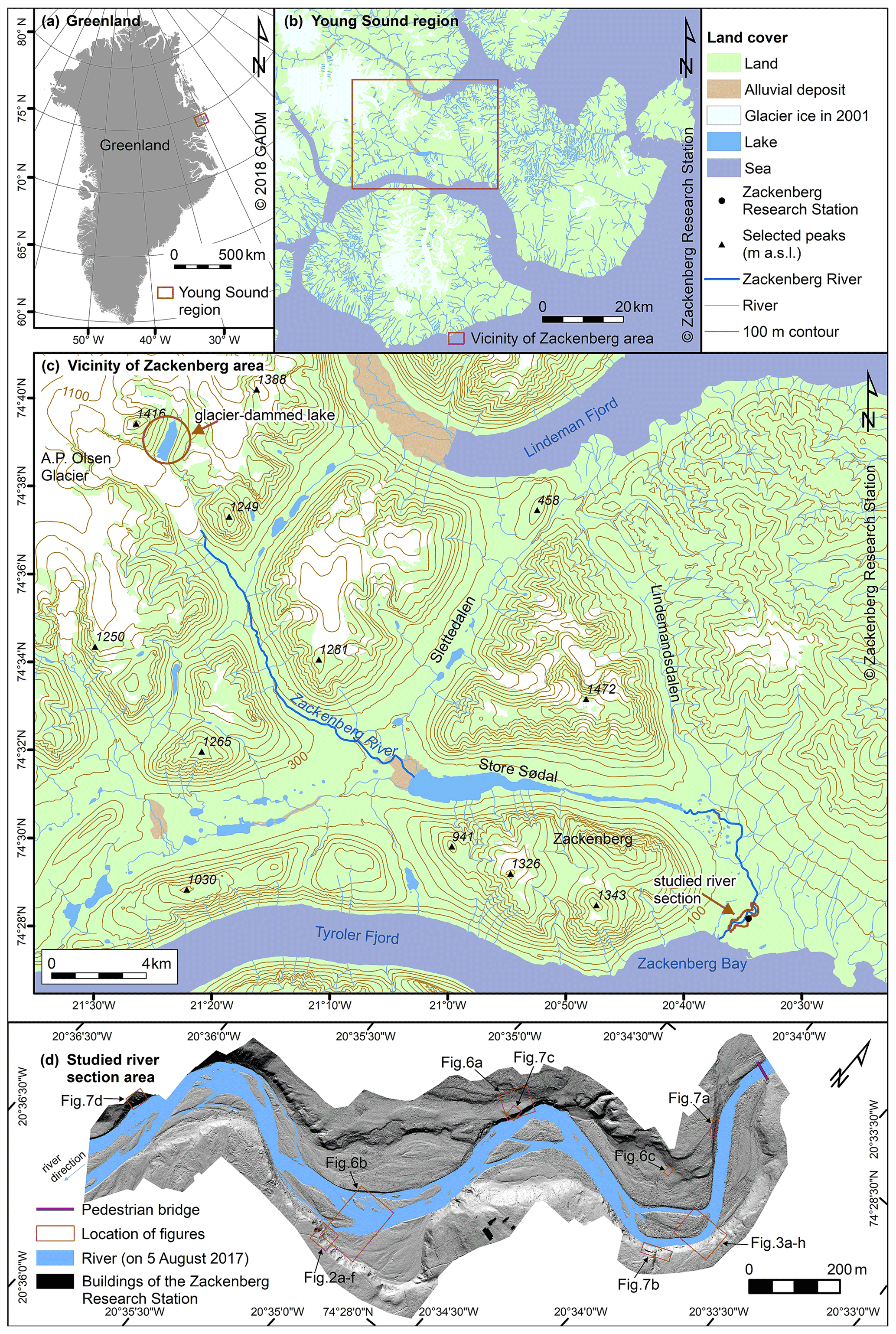
Figure 1Location of the study area (reprinted from Tomczyk et al., 2020, with permission from Elsevier, copyright 2020). Panel (d) shows survey area with extent of Figs. 2, 3, 6, and 7 indicated with boxes.
2.2 UAV surveys
According to the guidelines for using structure-from-motion (SfM) photogrammetry in geomorphological research (see James et al., 2019), details about UAV surveys are presented in Sect. 2.2, and the parameters used for SfM processing are detailed in Sect. 3. In that way, other researchers can use the data to replicate our results; alternatively, as new approaches become available, novel processing methods can be utilised.
2.2.1 Rationale
There were three primary goals for conducting the UAV surveys: (1) to collect data that would enable quantifying medium-term (i.e. temporal scale of several years) changes in the river landscape – compared to the available high-resolution 2014 data (COWI, 2015); (2) to document river state and immediate landscape response during the 2017 flood; and (3) to establish a baseline for the monitoring of geomorphological changes in response to future glacier lake outburst floods, including potential geohazards to research infrastructure (i.e. bridge and buildings of the research station). To achieve these aims, it was necessary to collect data with high spatial resolution, preferably better than 0.05 m ground sampling distance (GSD) (Fig. 2), covering a 2.1 km long section of the river from the bridge to the delta.
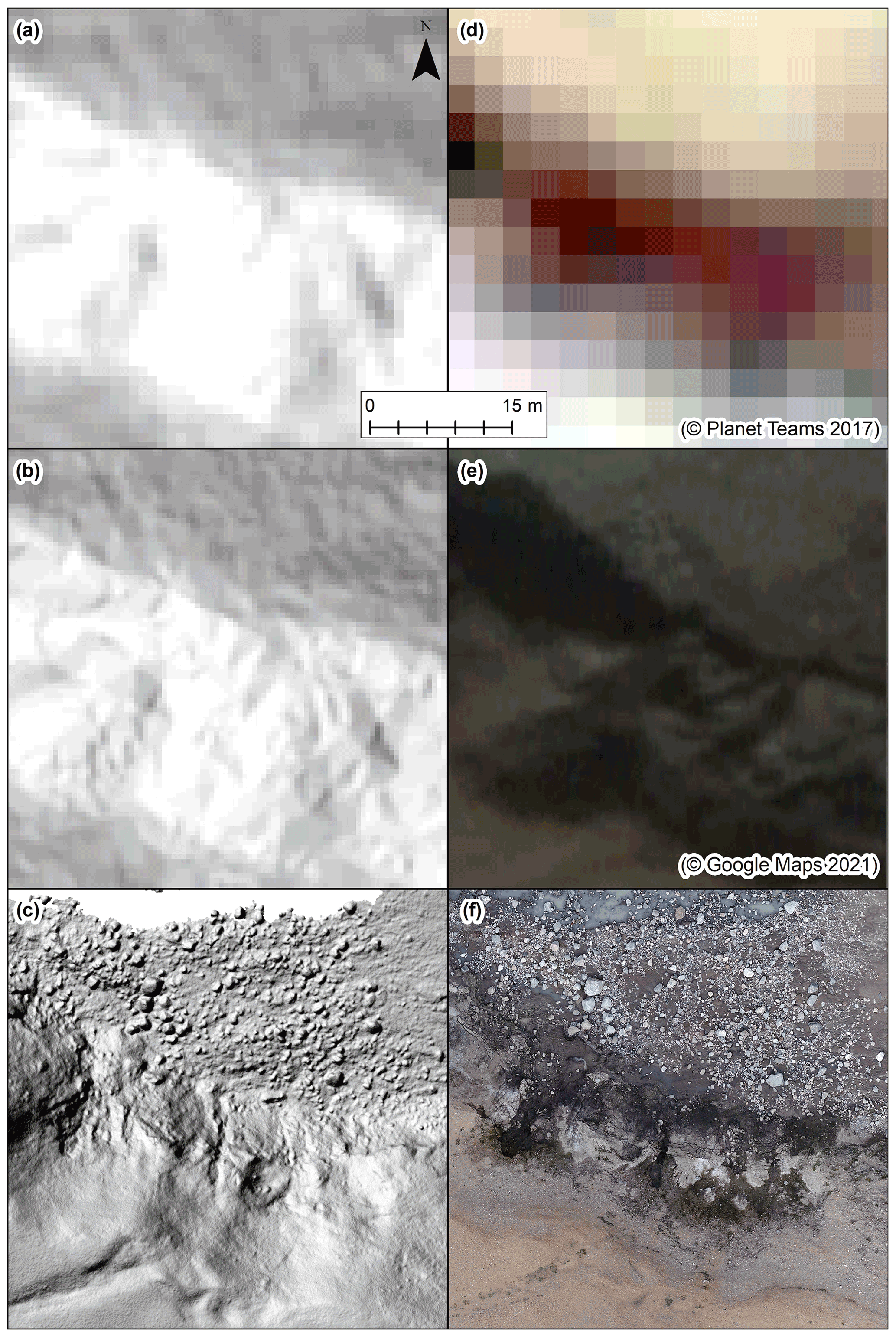
Figure 2Comparison of different data sources and their potential for mapping geomorphological features: (a) hillshade model 1 m GSD; (b) hillshade model 0.5 m GSD; (c) hillshade model 0.04 m GSD (generated from UAV-captured images); (d) Planet satellite imagery 3 m GSD (Planet Team, 2017); (e) high-resolution satellite image 0.5 m GSD (© Google Maps 2021); (f) orthomosaic 0.02 m GSD (generated from UAV-captured images).
2.2.2 Equipment
We used a lightweight, consumer-grade UAV – multirotor DJI Phantom 4 Pro. The low weight (1.4 kg) combined with a small size (0.35 m diagonal) ensures that the UAV could be easily transported in the field using a backpack – this was essential, as mechanised transport is not allowed due to fragility of the vegetation. The UAV was equipped with DJI 20MP, 1 in. size CMOS RGB sensor and a global shutter – camera model FC6310 (Table 1). There was a prime lens with 8.8 mm focal length (24 mm equivalent for 35 mm), aperture range from f/2.8 to f/11, and autofocus. A three-axis (pitch, roll, yaw) gimbal stabilised the camera, enabling it to take sharp pictures while the craft was in motion. The UAV was equipped with a global navigation satellite system (GNSS) receiver, capable of receiving signals from GPS and GLONASS satellite positioning systems.
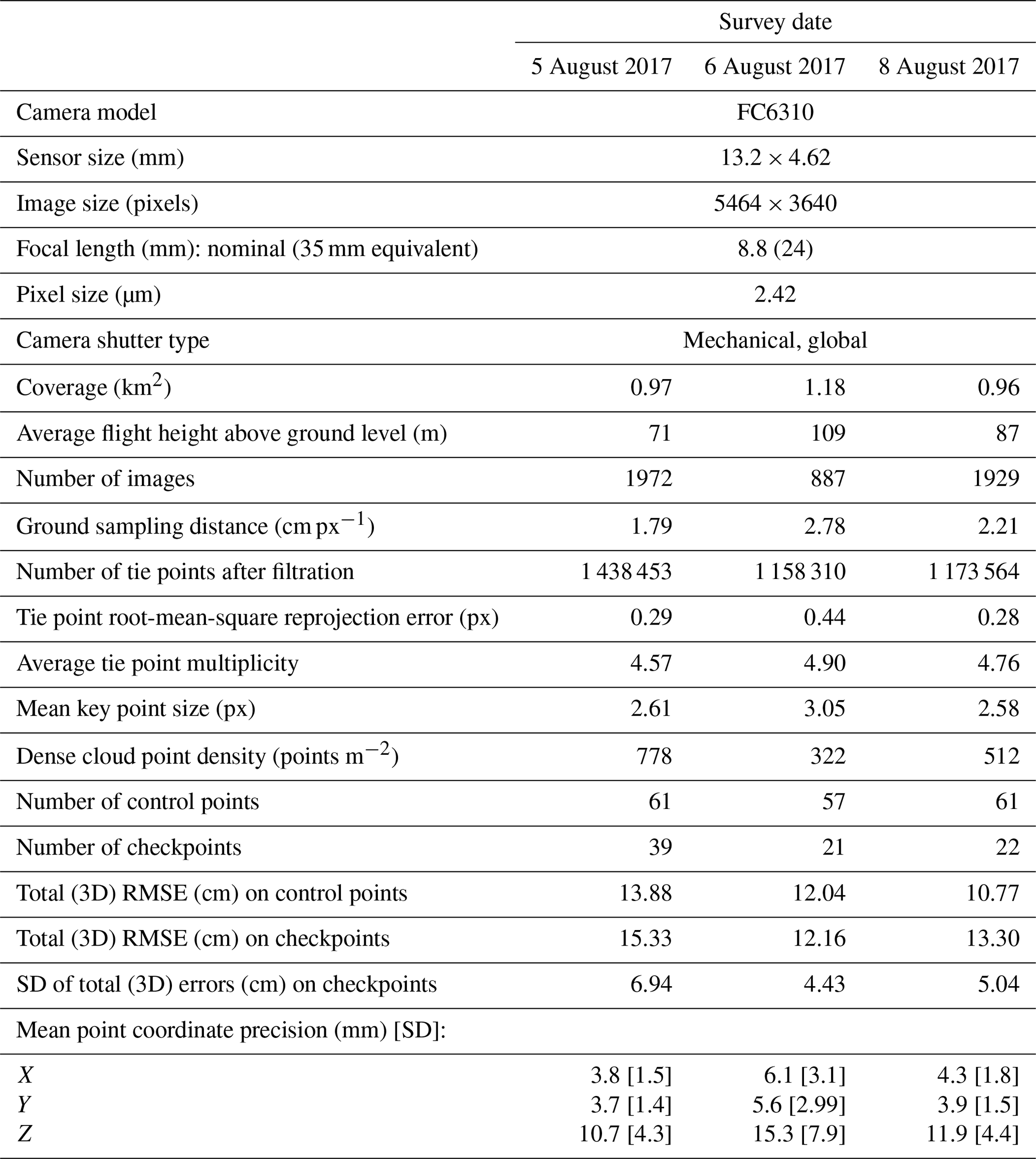
Table 1Outline of UAV surveys' parameters, processing errors, and final products' characteristics following the guidelines suggested by James et al. (2019).
2.3 Survey design and execution
To collect the necessary data, we designed an initial survey plan comprised of five lines approximately parallel to the main river channel's course routed over the centre of the main channel and both banks. During the surveys, this design was modified, as the river sections containing meandering segments were too wide to be captured with five lines of images with necessary overlap. Therefore, we turned to surveying N–S lines of the images, covering both the river channel and its neighbourhood.
Individual flights were operated manually, using DJI GO 4 app for Android, for in such high latitudes the on-board GNSS and magnetometer were potentially prone to erroneous reading. Related unexpected behaviours (e.g. errors in compass reading or loss of GNSS signal) were easier to tackle in the manual than automated mode. We captured mostly nadir images with a high overlap (>80 %). Additional oblique images were collected to cover the steep, near-vertical riverbank sections so as to ensure their proper representation in the model. Due to the length of the studied river section, and to comply with the visual line of sight (VLOS) flight operations, three take-off/landing sites were used each day. The weather condition for each day was good (i.e. no precipitation nor strong winds), and illumination conditions were sunny. The UAV surveys were performed at average nominal altitudes (from 70 to 110 m above ground level) to achieve the desired GSD (Table 1). In total, 1972 images were taken on 5 August 2017 (before-flood dataset), 887 images on 6 August 2017 (during-flood dataset), and 1929 images on 8 August 2017 (after-flood dataset). As the river level was fluctuating during the flood (6 August survey), we used a higher flight altitude, which translated into a lower number of images captured on 6 August but enabled us to cover the area more quickly with approximately the same water level during the survey. Therefore, it was a compromise between photogrammetric quality (i.e. the image network geometry), desired GSD, and rapidly changing flood conditions.
The unprocessed images captured during the surveys are available at https://doi.org/10.5281/zenodo.4495282 (Tomczyk and Ewertowski, 2021a). They can be used by interested parties to generate their own photogrammetric products using different methods and/or software than those described in Sect. 3.
3.1 Structure-from-motion processing
The UAV-captured images were processed using Agisoft Metashape Professional Edition 1.5.2. The values used for processing settings in each step were the following.
-
Camera settings. Camera type: frame; enable rolling shutter compensation: unchecked (as the UAV was equipped with global shutter).
-
Image alignment and sparse point cloud generation. Accuracy: high; generic preselection: yes; reference preselection: yes; key point limit: 100 000; tie point limit: 0 (i.e. unlimited).
-
Gradual selection and removal of the outliers and erroneous points. Three-stage selection based on reconstruction uncertainty: 10; reprojection error: 0.5; projection accuracy: 6.
-
Optimisation of the sparse point cloud. Parameters: f, B1, B2, cx, cy, K1, K2, P1, and P2.
-
Dense point cloud generation. Quality: high; depth filtering: aggressive.
-
DEM generation. Source data: dense cloud; interpolation: enabled.
The external orientation of the reconstructed scene was established using coordinates of each camera position obtained from the on-board GNSS system. To further constrain the geometry of the scene, additional control points (CPs) were used. As we were not able to collect high-quality ground control points (we did not have access to centimetre-accuracy survey equipment, and it was not possible to cross the river during the flood, because of the high water level), CPs were then generated post-survey using previous UAV dataset from 2014 (COWI, 2015). In total, 100 points were selected, located mostly on stable, flat boulders, which were easy to identify in the images. CPs were distributed on level terrain to minimise the impact of potential permafrost creep. Distribution of CPs was along both sides of the river to ensure that the distance between individual points is less than 100 m, which was suggested as optimal by Tonkin and Midgley (2016). The projection used was UTM 27N. The number of points used as control to optimise the exterior orientation was 61 (5 August), 57 (6 August), and 61 (8 August). The remaining points were used as independent checkpoints: 39 (5 August), 21 (6 August), and 22 (8 August). A smaller number of points used for data collected on 6 and 8 August were related to differences in coverage.
3.2 SfM processing results
The produced tie points clouds consisted of between 1.2 million (6 and 8 August) and 1.4 million (5 August) filtered points, with low tie point reprojection errors from 0.28 to 0.44 px, which was indicative of the high quality of the image geometry network (Table 1). Dense cloud point density varied from 322 points m−2 (6 August) to 778 points m−2 (5 August). These translated to orthomosaics with GSDs from 0.018 m (5 August) to 0.028 m (6 August) and DEMs with GSDs from 0.036 to 0.056 m (Fig. 3). The RMSEs for control points and checkpoints were between 0.12 and 0.15 m, which was expected, as the control points and checkpoints were transferred from previously existing data. The coherence between models was also estimated based on test areas selected in stable fragments of moraine and palaeo-delta to ensure significant systematic differences in elevation between datasets do not exist. The final products of SfM processing (orthomosaic and DEMs) and their derivative (hillshade models) for each data are available at https://doi.org/10.5281/zenodo.4498296 (Tomczyk and Ewertowski, 2021b).
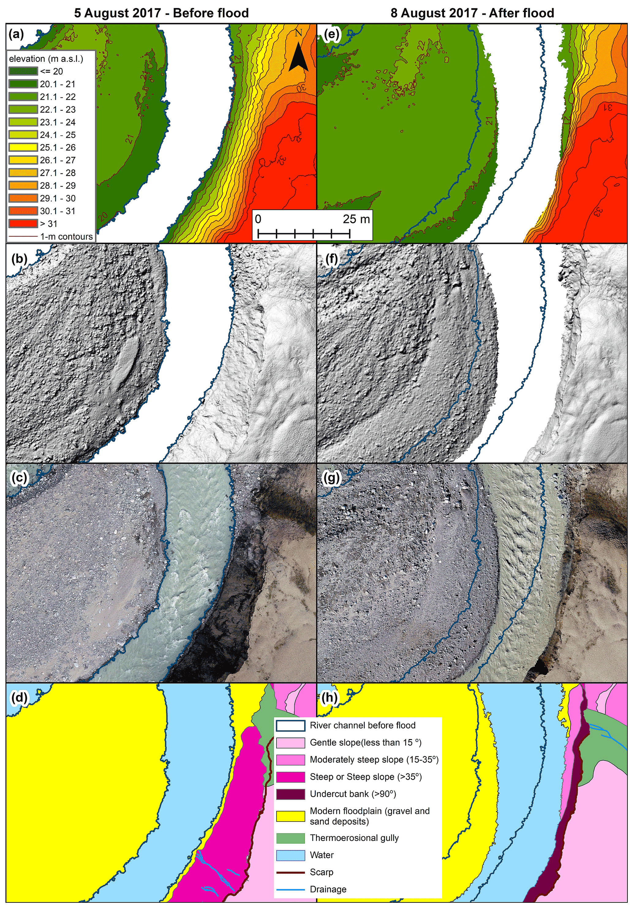
Figure 3Examples of the delivered dataset illustrating before and after the flood situation: (a, e) digital elevation model; (b, f) hillshade model; (c, g) orthomosaics; (d, h) results of geomorphological mapping.
3.3 Mapping
The mapping process was based on the approach proposed by Chandler et al. (2018); i.e. identification and interpretation of the geomorphological features were based on a combined analysis of remote sensing products and their derivatives (orthomosaics, DEMs, slope maps, hillshade models) as well as ground truthing. Final shapefile datasets were vectorised on-screen in ArcMap 10.6 software. The main geomorphological units (e.g. relict fluvial terraces, modern floodplain, slopes) and areas affected by mass movements of various types (e.g. debris flows, debris slumps) were mapped as polygons. Additional layers of polylines included features such as scarps or thermal-contraction cracks. River extent (i.e. area covered by water) is provided for each day as a separate polygon layer. Geomorphological features are provided as a separate file for before-the-flood (5 August 2017) and after-the-flood (8 August 2017) datasets. The mapping results in the form of vector files in the SHP format (compatible with most GIS software) are available to download from https://doi.org/10.5281/zenodo.4498296 (Tomczyk and Ewertowski, 2021b). Vector data combined with the hillshade models were presented as a series of geomorphological maps (see Tomczyk and Ewertowski, 2020, for details).
The quality of the presented datasets was assessed in relation to the outside world (i.e. external or absolute accuracy) and in relation to each survey (internal precision). Quality assessment based on data presented in Table 1 indicates a high quality of internal image network geometry, illustrated by low sub-pixel values of tie point reprojection errors. The external accuracy was estimated based on root-mean-square errors (RMSEs) and standard deviations (SDs) of errors on checkpoints, which were between 0.12 and 0.15 m (Table 1). The maximum external error for two checkpoints was −0.4 and 0.4 m. Although such values are higher than the GSD of all datasets (between 0.018 and 0.028 m), such magnitude of errors was considered acceptable for the quantification and mapping of landscape changes, especially as between 5 and 8 August the resultant lateral erosion of riverbanks from the flood reached almost 10 m in some sections (see Tomczyk et al., 2020, for details); therefore, the observed changes were up 100 times larger than RMSE. If necessary, lower values of absolute accuracy can be achieved in the future if additional ground control points are surveyed using a centimetre-accuracy survey equipment. Moreover, if better relative accuracy (i.e. survey-to-survey accuracy) is necessary in the future monitoring applications, co-alignment of UAV time series can provide better relative accuracy than the classic approach of individual SfM processing of each survey using ground control points (GCPs) – as demonstrated in several studies (e.g. Feurer and Vinatier, 2018; Cook and Dietze, 2019; de Haas et al., 2021). Therefore, we provided also unprocessed images so the potential user can perform their own SfM processing.
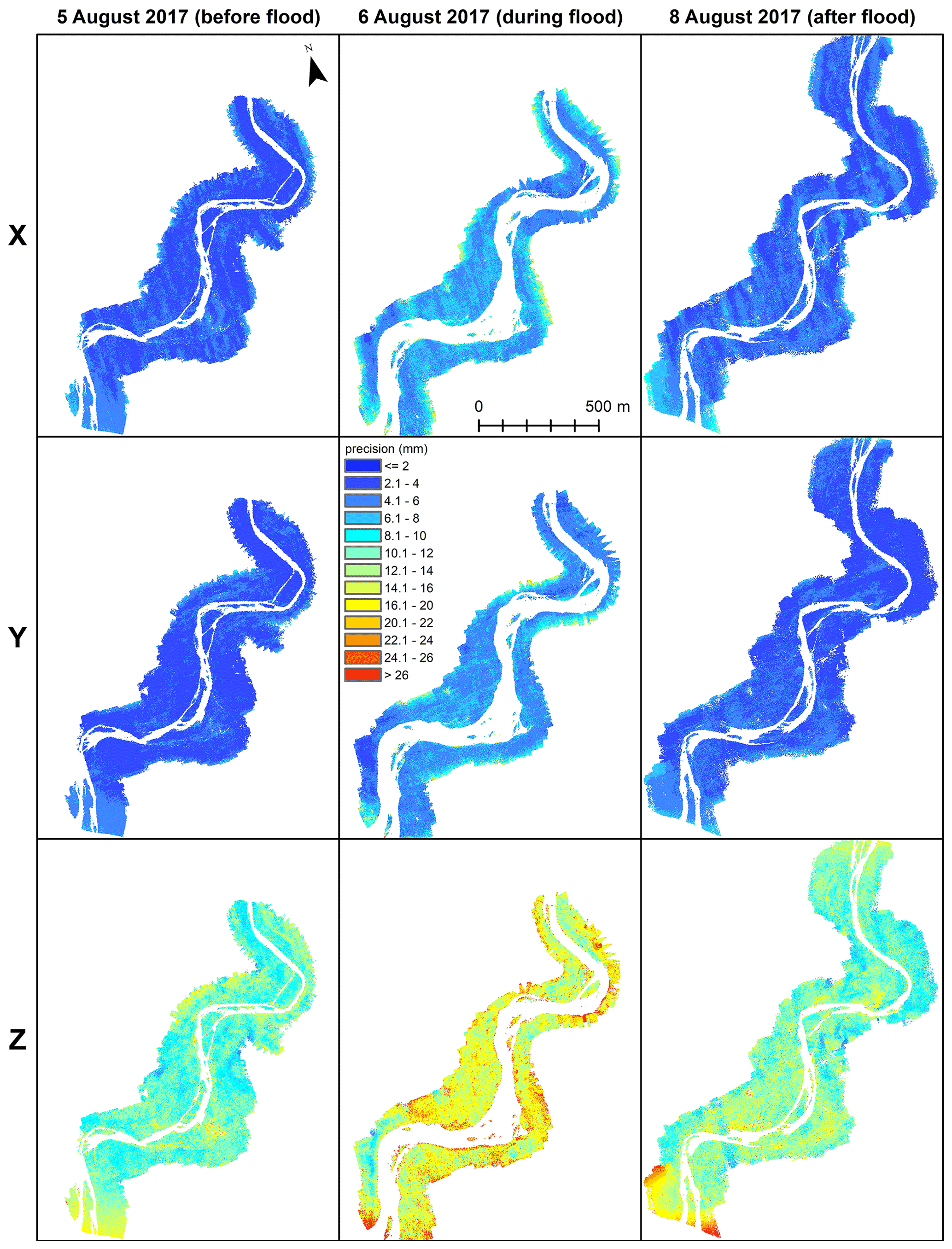
Figure 4Precision estimates for X, Y, and Z coordinates of tie points. Location of the studied river section is presented in Fig. 1d.
The internal quality of the reconstructed scenes was based on tie point precision. To estimate the spatial variability of the models' photogrammetric and georeferencing uncertainties, the precision estimates for sparse point clouds were generated in Agisoft Metashape and exported using the Python script provided by James et al. (2020). The precision analysis indicated that the vertical component was less spatially consistent than the horizontal ones for all three surveys (Fig. 4). For the models' ground parts, the overall precision was limited by the precision of control points, which is not surprising as they were derived from the older, less detailed remote sensing dataset. The internal accuracy of each survey was assessed based on the mean point precision estimates, which varied from 4 to 6 mm for the horizontal component and from 11 to 15 mm for the vertical one (Table 1) – the weakest values were for the 6 August 2017 dataset, which was expected as the average flying altitude was highest then. Precision maps are available to download from https://doi.org/10.5281/zenodo.4498296 (Tomczyk and Ewertowski, 2021b). Z discrepancies on control points were calculated using Doming Analysis software (v.1.0) (James et al., 2020). The analysis indicated no doming distortion (Fig. 5), which is probably related to the generally very high overlap of images and the inclusion of oblique images of the steep riverbanks.
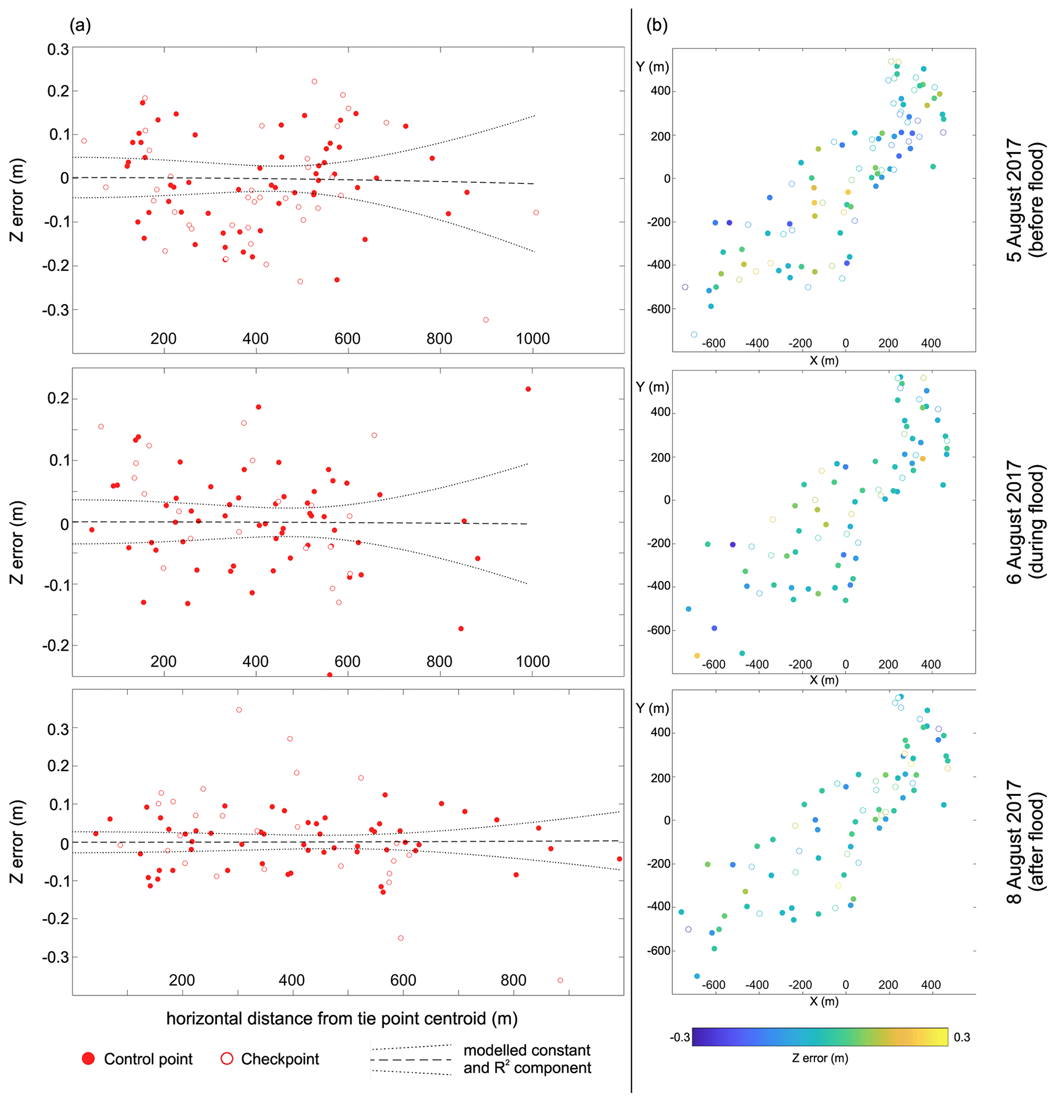
Figure 5Spatial distribution of errors on control points and checkpoints: (a) Z error against radial distance from the tie point cloud centroid (i.e. from the centre of the reconstructed scene). The distribution of errors along a straight line (indicated here also as “modelled constant”) suggests that no systematic errors such as doming or dishing were observed in the reconstructed scenes (see James et al., 2020, for details about interpretation); (b) Z error by colour in plan view (X and Y are distanced from tie point centroid). Note that each row shows an individual survey.
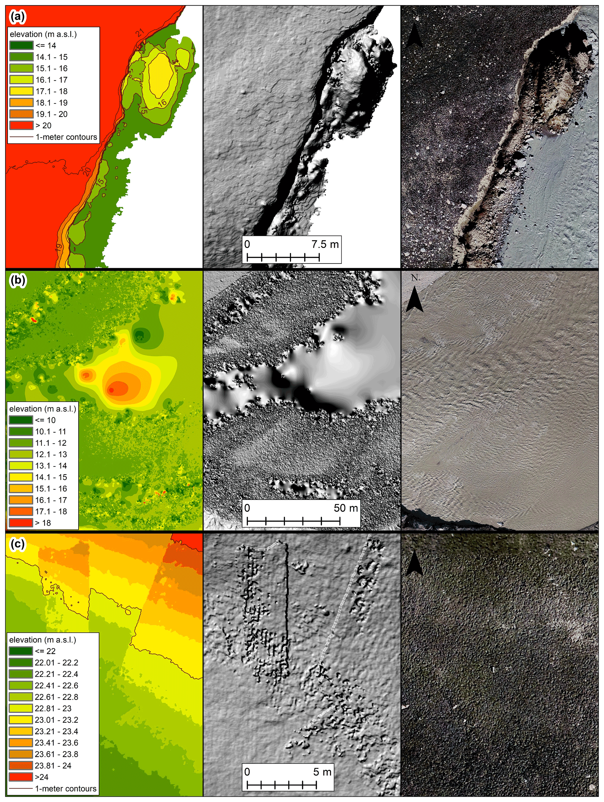
Figure 6Examples of encountered problems: (a) undercut/overhanging river sections; (b) rapidly moving water; (c) artefacts related to errors in surface reconstruction.
Individual orthomosaics and DEMs were also inspected, resulting in the discovery of the following problems, which ought to be taken into account in any future analysis.
-
In general, the interpretation of riverbank conditions can be influenced by vegetation cover and/or bank undercutting (Niedzielski et al., 2016; Hemmelder et al., 2018). While vegetation cover is usually not a problem in the case of Arctic rivers, other obstacles (e.g. shadows, infrastructure) might prevent the direct measurements of the bank's heights. In the case of the presented dataset, some sections of riverbanks were steep, near-vertical, before the flood (Figs. 6a and 7). However, during the flood, some of the sections were significantly undercut, forming deeply incised niches (Fig. 7) – these overhanging banks obstructed the view of the bottom part of some studied sections from the air. During the UAV campaigns, we took oblique images to at least produce a proper representation of steep slopes; however, it was not possible to take horizontal images due to the presence of water. As a result, it was impossible to calculate the volume of sediments eroded from the niches under these overhanging sections.
-
Structure-from-motion is based on reconstructing the image network geometry based on characteristic points that appear in several images (Westoby et al., 2012). It therefore fails where there are rapidly moving objects, which changed their position in time between the images captured. The structure-from-motion photogrammetry can reconstruct the location of points in dry areas and, in the case of transparent water, also points located underwater (Carrivick and Smith, 2019). However, in our study, the high turbidity of water and sediment suspension prevented viewing of the riverbed. As an Arctic river, the Zackenberg River has suspended sediment concentrations within a range of 50 to 500 mg L−1 (Søndergaard et al., 2015), which can increase even up to 4000 mg L−1 during glacial lake outburst floods, indicated by the lack of transparency and the yellow or brown colours of water in the orthomosaics. The turbidity of water is also very high (Ladegaard-Pedersen et al., 2017), as was also found in our surveys. The fact that the water surface was full of ripples gave rise to bidirectional reflectance problems. Therefore, it was not possible to adequately resolve the surface of flowing water (Fig. 6b). To partly address this issue, the water bodies were masked from DEMs and hillshade models. They are, however, visible in orthomosaics, which enables the user to assess the character of water flow (Fig. 8).
-
Some fragments of the models revealed artefacts associated with mismatches in point generation. These areas can generate erroneous elevation values, which can be identified in the DEM and hillshade model as unexpectedly rough surfaces in places where the ground level should be uniform (Fig. 6c). These areas were indicated with polygon files for easy identification in case of future analysis.
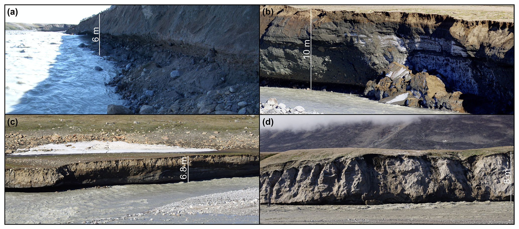
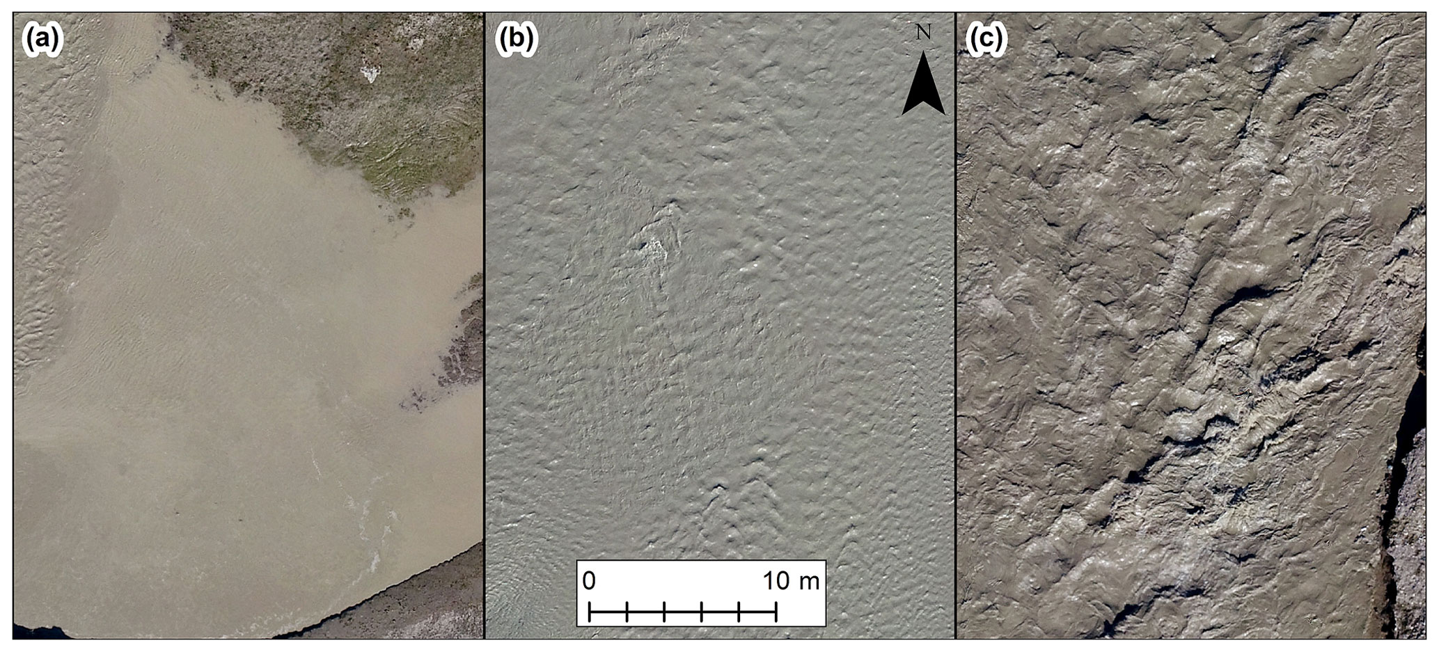
Figure 8Different character of water surfaces: (a) stagnant and slow flowing water; (b) moderate flow rate; (c) rapid, turbulent water flow.
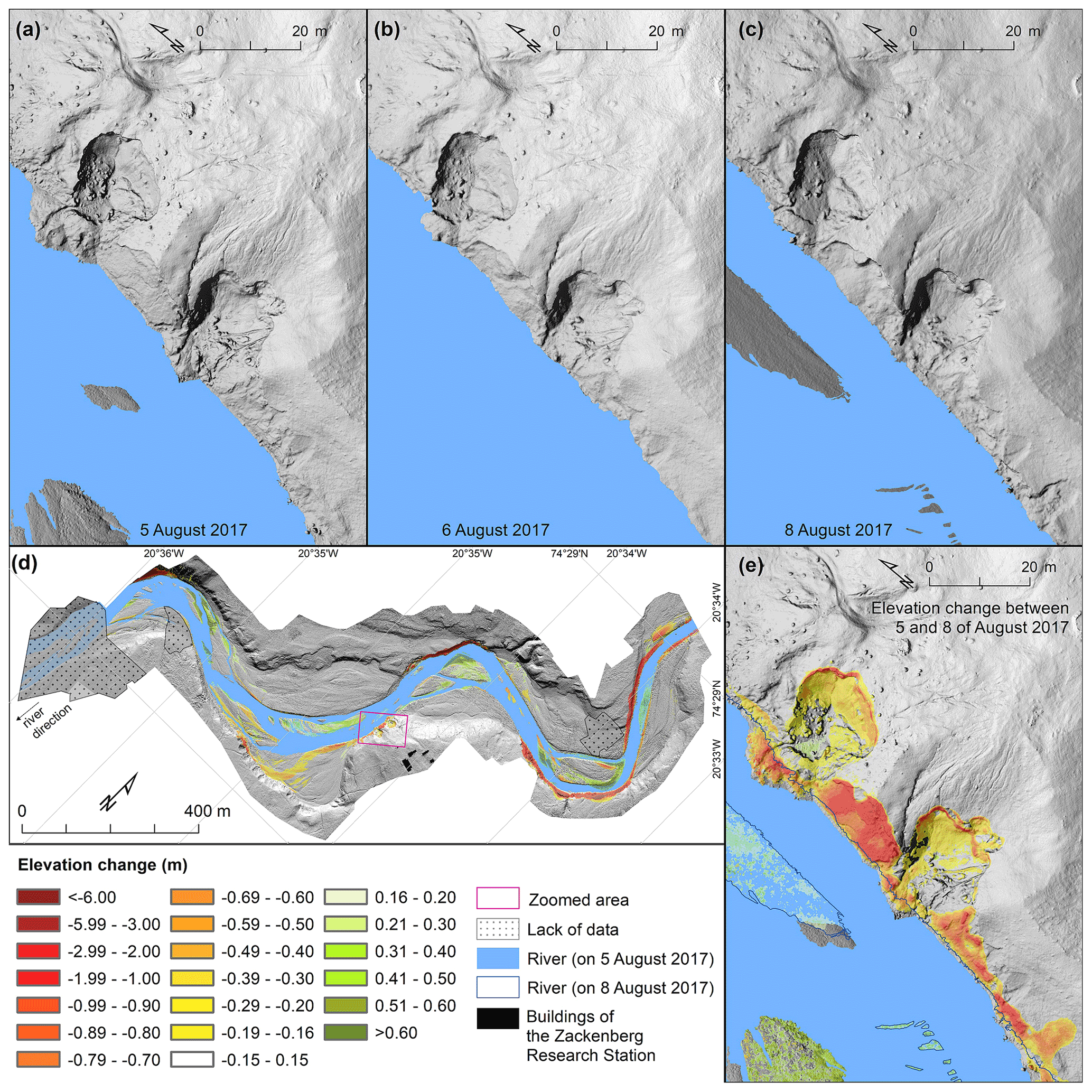
Figure 9Examples of DEM of Differences demonstrating geomorphic change detection for two debris flows located in the vicinity of the Zackenberg Research Station.
All described data are available in the Zenodo repository. The structure of the dataset is as follows.
-
Unprocessed UAV-captured images (∼46 GB) are available at https://doi.org/10.5281/zenodo.4495282 (Tomczyk and Ewertowski, 2021a). The images are zipped into three folders following naming convention: 2017_08_05_before_flood_unprocessed_UAV_images, 2017_08_06_during_flood_unprocessed_UAV_images, and 2017_08_08_after_flood_unprocessed_UAV_images. The images are in JPG format and contain embedded positions in geographic coordinate system WGS84 obtained from the on-board GNSS receiver.
-
The results of photogrammetric processing (∼ 18 GB) are available at https://doi.org/10.5281/zenodo.4498296 (Tomczyk and Ewertowski, 2021b) in the file Sfm_products.zip and are grouped into subfolders with the following names: dem (containing digital elevation models), orthomosaic (containing orthomosaics), and hs (containing hillshade models); all data are in GeoTIFF format in the UTM 27N projected coordinate system. Individual files are named as follows: yyyy_mm_dd_[filetype]_[status].tif, where
- a.
yyyy_mm_dd is a date, e.g. 2017_08_05;
- b.
[filetype] represents the possible values dem (= DEM), ortho (= orthomosaic), and hs (= hillshade); and
- c.
[status] represents the possible values before_flood, during_flood, and after_flood.
- a.
-
The mapping results (25 MB) are in the same repository entry as SfM processing results, i.e. at https://doi.org/10.5281/zenodo.4498296 (Tomczyk and Ewertowski, 2021b) in the folder “mapping.zip”. Inside, there are four subfolders:
- a.
General, which contains general vectors that did not change over the course of 3 d (e.g. station buildings, 4x4 trail);
- b.
River_extent, which contains polygons for river extent for 2014 (generated from older UAV data (COWI, 2015)) and for 5, 6, and 8 August 2017 – the 2017 data are named as yyyy_mm_dd_river;
- c.
Before_flood_geomorphology, which contains polygon and lines illustrating geomorphological features before the flood, with separate files providing extent of mass movements which can be potentially hazardous, e.g. debris flows, debris falls, rockfalls, and slumps (names of individual files are provided in Table 2); and
- d.
After_flood_geomorphology, which contains polygons and lines illustrating geomorphological features after the flood, with separate files providing extent of mass movements which can be potentially hazardous, e.g. debris flows, debris falls, rockfalls, and slumps (names of individual files are provided in Table 2).
All data are in SHP vector format in the UTM 27N projected coordinate system.
- a.
-
Precision estimates for tie points and precision maps for X, Y, and Z coordinates are in the same repository entry as SfM processing results, i.e. at https://doi.org/10.5281/zenodo.4498296 (Tomczyk and Ewertowski, 2021a) in the folder “uncertainty_assessment.zip”. Individual files are named as follows:
- a.
yyyy_mm_dd_[before_flood/during_flood/after_flood]_points_precision.txt, which contain precision estimates for each tie point; and
- b.
yyyy_mm_dd_[before_flood/during_flood/after_flood]_[X/Y/Z]_precision.tif, which contain precision estimates for each coordinate as raster file.
- a.
Structure-from-motion processing was performed in the proprietary software Agisoft Metashape (https://www.agisoft.com/, Agisoft, 2021). Mapping was performed in ArcMap (https://www.esri.com/en-us/arcgis/about-arcgis/overview, Esri, 2021). Python script exporting precision estimates from Agisoft Metashape and Doming Analysis software (v.1.0) (James et al., 2020) are available to download from https://www.lancaster.ac.uk/staff/jamesm/software/sfm_georef.htm.
Table 2List of filenames for corresponding dates and content.

The ability to detect changes in the geomorphology of the riverbed and riparian areas remains a crucial issue in monitoring and modelling the geomorphic effects of flood events. Using a UAV survey for rapid assessment, as in the case of the studied 2017 flood, can be more beneficial than other methods (like high-resolution satellite imagery, terrestrial laser scanning) (cf. Carrivick et al., 2016; Smith et al., 2016), as it allows for covering the substantial length of the river with high-resolution data. Such data are intended to be a baseline for future monitoring projects. Potential applications of the presented dataset include the following.
-
Establishing a long-term monitoring of high-Arctic river valley development in a permafrost terrain. Climate warming in the Arctic is more intense than in other regions (see Moritz et al., 2002; Walsh et al., 2011; Duarte et al., 2012), with the thawing of permafrost in Greenland being one of the effects (Elberling et al., 2013; Anderson et al., 2017). In such a dynamic environment, riverscapes are also likely to transform rapidly (Chassiot et al., 2020). As our data cover the river section located close to the Zackenberg Research Station, it facilitates logistics and can potentially enable developing long-term remote sensing data series illustrating the dynamic response of the riverscape to ongoing climate change, which is essential from the standpoint of long-term landscape evolution.
-
Quantification, monitoring, and modelling of geomorphological impacts of glacier lake outburst flood. The presented dataset was meant to quantify changes related to the 2017 GLOF (see Tomczyk and Ewertowski, 2020; Tomczyk et al., 2020); however, these studies only described the immediate impacts of a single flood event. An example of geomorphic change detection is presented in Fig. 9, demonstrating the acceleration of debris flows resulting from sediment entrainment at the base of the river banks by floodwater. Overall, the observed changes were spatially variable – erosion dominated along steep banks as expected; however, understanding of differences in erosion rates between sites requires further studies, which will consider differences in lithology as well as modelling of water flow to investigate potential erosion forces in relation to channel characteristics. The first GLOF at Zackenberg was observed in 1996, and since then floods occurred every year or at 2-year intervals (Kroon et al., 2017; Tomczyk and Ewertowski, 2020). The lake, which is the source of GLOF, is located more than 3 km from the current ice margin, so we expect a similar or higher frequency of floods as more water will be melting from glaciers and stored in the lake. Thus, future monitoring is needed to investigate whether the GLOFs will be observed more frequently but with lower discharge magnitude or less often but with higher discharge.
-
Process-based modelling studies. As the high-magnitude, low-frequency events are typically rare and difficult to predict, our understanding of the quantitative aspect of geomorphological changes related to them remains limited compared to the normal processes (Tamminga et al., 2015a). These arise particularly from difficulties in collecting high-resolution data before and after these innately unpredictable and rare flood events. However, investigation into the geomorphological response of river morphology to extreme events is key to understanding the evolution of river morphology and crucial from the standpoint of river modelling and monitoring (Tamminga et al., 2015a, b). Moreover, the relationship between the magnitude of the flood and geomorphological effects is not fully understood. For example, in the case of Zackenberg River, immediate (2 d) lateral erosion compared to 3-year erosion was spatially very diversified. In some sections, immediate lateral erosion after the 2017 flood reached up to 10 m, whereas the same section was stable between 2014 and 2017, even though higher peak discharges characterised 2015 and 2016 GLOFs compared to 2017 GLOF (Tomczyk et al., 2020). Further process-based studies are necessary to observe and model links between the magnitude of a flood and the severity of erosion. It is especially important in periglacial landscapes where lateral bank erosion can be responsible for delivering a large quantity of organic matter and widespread changes in ecosystems, especially combined with other weather extreme events (see Christensen et al., 2021). Using the provided dataset as a baseline for the monitoring of future changes, it should be possible to quantify the difference between geomorphological effects of normal (i.e. high-frequency, low-magnitude) processes on the one hand and extreme (i.e. low-frequency, high-magnitude) events on the other. Also, by linking the intensity of a geomorphological response to hydrological data about flood characteristics, it should be possible to improve modelling routines (see Carrivick, 2007a, b; Carrivick et al., 2011; Guan et al., 2015; Staines and Carrivick, 2015).
-
Geohazard assessment. The Zackenberg Research Station premises are located close to the riverbank, which is regularly affected by floods. The development of debris flows, which has started to threaten the station's infrastructure, is one outcome of the removal of sediments from the channel by flood. Another example of geohazards is the washing out of the foundation of the bridge located up the valley. These hazards require regular monitoring to prevent damage to the infrastructure, and the presented database can be used to assess current hazards and establish a baseline for future monitoring.
AMT and MWE collected data during the field campaign and performed the photogrammetric processing and uncertainty analysis. AMT mapped the geomorphology and wrote the paper with input from MWE.
The authors declare that they have no conflict of interest.
Publisher's note: Copernicus Publications remains neutral with regard to jurisdictional claims in published maps and institutional affiliations.
We are very grateful for the support from INTERACT network, which allowed us to visit Zackenberg Research Station in 2017. The realisation of the fieldwork would not have been possible without logistic support provided by the crew of the Zackenberg Research Station.
This research has been supported by the Horizon 2020 project INTERACT (grant no. 730938, project number 119 (ArcticFan)).
This paper was edited by Alexander Gelfan and reviewed by Dmitry Petrakov and three anonymous referees.
Agisoft: Homepage, available at: https://www.agisoft.com/, last access: 9 November 2021.
Anderson, N. J., Saros, J. E., Bullard, J. E., Cahoon, S. M. P., McGowan, S., Bagshaw, E. A., Barry, C. D., Bindler, R., Burpee, B. T., Carrivick, J. L., Fowler, R. A., Fox, A. D., Fritz, S. C., Giles, M. E., Hamerlik, L., Ingeman-Nielsen, T., Law, A. C., Mernild, S. H., Northington, R. M., Osburn, C. L., Pla-Rabès, S., Post, E., Telling, J., Stroud, D. A., Whiteford, E. J., Yallop, M. L., and Yde, J. C.: The Arctic in the Twenty-First Century: Changing Biogeochemical Linkages across a Paraglacial Landscape of Greenland, Bioscience, 67, 118–133, https://doi.org/10.1093/biosci/biw158, 2017.
Behm, M., Walter, J. I., Binder, D., and Mertl, S.: Seismic Monitoring and Characterization of the 2012 Outburst Flood of the Ice-Dammed Lake A.P. Olsen (NE Greenland), AGU Fall Meeting 2017, New Orleans, 11–15 December 2017, C41D-0432, available at: https://ui.adsabs.harvard.edu/abs/2017AGUFM.C41D1260B (last access: 9 November 2021), 2017.
Behm, M., Walter, J. I., Binder, D., Cheng, F., Citterio, M., Kulessa, B., Langley, K., Limpach, P., Mertl, S., Schöner, W., Tamstorf, M., and Weyss, G.: Seismic characterization of a rapidly-rising jökulhlaup cycle at the A.P. Olsen Ice Cap, NE-Greenland, J. Glaciol., 66, 329–347, https://doi.org/10.1017/jog.2020.9, 2020.
Bendixen, M., Lønsmann Iversen, L., Anker Bjørk, A., Elberling, B., Westergaard-Nielsen, A., Overeem, I., Barnhart, K. R., Abbas Khan, S., Box, J. E., Abermann, J., Langley, K., and Kroon, A.: Delta progradation in Greenland driven by increasing glacial mass loss, Nature, 550, 101–104, https://doi.org/10.1038/nature23873, 2017.
Carrivick, J. L.: Modelling coupled hydraulics and sediment transport of a high-magnitude flood and associated landscape change, Ann. Glaciol., 45, 143–154, https://doi.org/10.3189/172756407782282480, 2007a.
Carrivick, J. L.: Hydrodynamics and geomorphic work of jökulhlaups (glacial outburst floods) from Kverkfjöll volcano, Iceland, Hydrol. Process., 21, 725–740, https://doi.org/10.1002/hyp.6248, 2007b.
Carrivick, J. L. and Smith, M. W.: Fluvial and aquatic applications of Structure from Motion photogrammetry and unmanned aerial vehicle/drone technology, WIREs Water, 6, e1328, https://doi.org/10.1002/wat2.1328, 2019.
Carrivick, J. L. and Tweed, F. S.: A global assessment of the societal impacts of glacier outburst floods, Global Planet. Change, 144, 1–16, https://doi.org/10.1016/j.gloplacha.2016.07.001, 2016.
Carrivick, J. L. and Tweed, F. S.: A review of glacier outburst floods in Iceland and Greenland with a megafloods perspective, Earth-Sci. Rev., 196, 102876, https://doi.org/10.1016/j.earscirev.2019.102876, 2019.
Carrivick, J. L., Russell, A. J., and Tweed, F. S.: Geomorphological evidence for jökulhlaups from Kverkfjöll volcano, Iceland, Geomorphology, 63, 81–102, https://doi.org/10.1016/j.geomorph.2004.03.006, 2004.
Carrivick, J. L., Jones, R., and Keevil, G.: Experimental insights on geomorphological processes within dam break outburst floods, J. Hydrol., 408, 153–163, https://doi.org/10.1016/j.jhydrol.2011.07.037, 2011.
Carrivick, J. L., Turner, A. G. D., Russell, A. J., Ingeman-Nielsen, T., and Yde, J. C.: Outburst flood evolution at Russell Glacier, western Greenland: effects of a bedrock channel cascade with intermediary lakes, Quaternary Sci. Rev., 67, 39–58, https://doi.org/10.1016/j.quascirev.2013.01.023, 2013.
Carrivick, J. L., Smith, M. W., and Quincey, D. J.: Structure from Motion in the Geosciences, Analytical Methods in Earth and Environmental Science, Wiley-Blackwell, Oxford, UK, 208 pp., 2016.
Carrivick, J. L., Tweed, F. S., Ng, F., Quincey, D. J., Mallalieu, J., Ingeman-Nielsen, T., Mikkelsen, A. B., Palmer, S. J., Yde, J. C., Homer, R., Russell, A. J., and Hubbard, A.: Ice-Dammed Lake Drainage Evolution at Russell Glacier, West Greenland, Front. Earth Sci., 5, 100, https://doi.org/10.3389/feart.2017.00100, 2017.
Chandler, B. M. P., Lovell, H., Boston, C. M., Lukas, S., Barr, I. D., Benediktsson, Í. Ö., Benn, D. I., Clark, C. D., Darvill, C. M., Evans, D. J. A., Ewertowski, M. W., Loibl, D., Margold, M., Otto, J.-C., Roberts, D. H., Stokes, C. R., Storrar, R. D., and Stroeven, A. P.: Glacial geomorphological mapping: A review of approaches and frameworks for best practice, Earth-Sci. Rev., 185, 806–846, https://doi.org/10.1016/j.earscirev.2018.07.015, 2018.
Chassiot, L., Lajeunesse, P., and Bernier, J.-F.: Riverbank erosion in cold environments: Review and outlook, Earth-Sci. Rev., 207, 103231, https://doi.org/10.1016/j.earscirev.2020.103231, 2020.
Christensen, T. R., Lund, M., Skov, K., Abermann, J., López-Blanco, E., Scheller, J., Scheel, M., Jackowicz-Korczynski, M., Langley, K., Murphy, M. J., and Mastepanov, M.: Multiple Ecosystem Effects of Extreme Weather Events in the Arctic, Ecosystems, 24, 122–136, https://doi.org/10.1007/s10021-020-00507-6, 2021.
Cook, K. L. and Dietze, M.: Short Communication: A simple workflow for robust low-cost UAV-derived change detection without ground control points, Earth Surf. Dynam., 7, 1009–1017, https://doi.org/10.5194/esurf-7-1009-2019, 2019.
Cook, K. L., Andermann, C., Gimbert, F., Adhikari, B. R., and Hovius, N.: Glacial lake outburst floods as drivers of fluvial erosion in the Himalaya, Science, 362, 53–57, https://doi.org/10.1126/science.aat4981, 2018.
COWI: Mapping Greenland's Zackenberg Research Station, available at: https://www.sensefly.com/app/uploads/2017/11/eBee_saves_day_mapping_greenlands_zackenberg_research_station.pdf (last access: 9 November 2021), 2015.
Dawson, A. G.: Glacier-dammed lake investigations in the Hullet Lake area, South Greenland, in: Medd. Grønl. Geosci., 11, The Commission for Scientific Research in Greenland, Denmark, Copenhagen, 24 pp., ISBN 8763511584, 1983.
Death, R. G., Fuller, I. C., and Macklin, M. G.: Resetting the river template: the potential for climate-related extreme floods to transform river geomorphology and ecology, Freshwater Biol., 60, 2477–2496, https://doi.org/10.1111/fwb.12639, 2015.
de Haas, T., Nijland, W., McArdell, B. W., and Kalthof, M. W. M. L.: Case Report: Optimization of Topographic Change Detection With UAV Structure-From-Motion Photogrammetry Through Survey Co-Alignment, Frontiers in Remote Sensing, 2, 626810, https://doi.org/10.3389/frsen.2021.626810, 2021.
Desloges, J. R. and Church, M.: Geomorphic implications of glacier outburst flooding: Noeick River valley, British Columbia, Can. J. Earth Sci., 29, 551–564, https://doi.org/10.1139/e92-048, 1992.
Duarte, C. M., Lenton, T. M., Wadhams, P., and Wassmann, P.: Abrupt climate change in the Arctic, Nat. Clim. Change, 2, 60–62, https://doi.org/10.1038/nclimate1386, 2012.
Elberling, B., Michelsen, A., Schädel, C., Schuur, E. A. G., Christiansen, H. H., Berg, L., Tamstorf, M. P., and Sigsgaard, C.: Long-term CO2 production following permafrost thaw, Nat. Clim. Change, 3, 890–894, https://doi.org/10.1038/nclimate1955, 2013.
Esri: ArcGis, Esri [software], available at: https://www.esri.com/en-us/arcgis/about-arcgis/overview, last access: 9 November 2021.
Feurer, D. and Vinatier, F.: Joining multi-epoch archival aerial images in a single SfM block allows 3-D change detection with almost exclusively image information, ISPRS J. Photogramm., 146, 495–506, https://doi.org/10.1016/j.isprsjprs.2018.10.016, 2018.
Furuya, M. and Wahr, J. M.: Water level changes at an ice-dammed lake in west Greenland inferred from InSAR data, Geophys. Res. Lett., 32, L14501, https://doi.org/10.1029/2005GL023458, 2005.
Garcia-Castellanos, D. and O'Connor, J. E.: Outburst floods provide erodability estimates consistent with long-term landscape evolution, Scientific Reports, 8, 10573, https://doi.org/10.1038/s41598-018-28981-y, 2018.
Grinsted, A., Hvidberg, C. S., Campos, N., and Dahl-Jensen, D.: Periodic outburst floods from an ice-dammed lake in East Greenland, Scientific Reports, 7, 9966, https://doi.org/10.1038/s41598-017-07960-9, 2017.
Guan, M., Wright, N. G., Sleigh, P. A., and Carrivick, J. L.: Assessment of hydro-morphodynamic modelling and geomorphological impacts of a sediment-charged jökulhlaup, at Sólheimajökull, Iceland, J. Hydrol., 530, 336–349, https://doi.org/10.1016/j.jhydrol.2015.09.062, 2015.
Harrison, S., Glasser, N., Winchester, V., Haresign, E., Warren, C., and Jansson, K.: A glacial lake outburst flood associated with recent mountain glacier retreat, Patagonian Andes, Holocene, 16, 611–620, https://doi.org/10.1191/0959683606hl957rr, 2006.
Harrison, S., Kargel, J. S., Huggel, C., Reynolds, J., Shugar, D. H., Betts, R. A., Emmer, A., Glasser, N., Haritashya, U. K., Klimeš, J., Reinhardt, L., Schaub, Y., Wiltshire, A., Regmi, D., and Vilímek, V.: Climate change and the global pattern of moraine-dammed glacial lake outburst floods, The Cryosphere, 12, 1195–1209, https://doi.org/10.5194/tc-12-1195-2018, 2018.
Hasholt, B., Mernild, S. H., Sigsgaard, C., Elberling, B., Petersen, D., Jakobsen, B. H., Hansen, B. U., Hinkler, J., and Søgaard, H.: Hydrology and Transport of Sediment and Solutes at Zackenberg, Adv. Ecol. Res., 40, 197–221, https://doi.org/10.1016/S0065-2504(07)00009-8 2008.
Hasholt, B., van As, D., Mikkelsen, A. B., Mernild, S. H., and Yde, J. C.: Observed sediment and solute transport from the Kangerlussuaq sector of the Greenland Ice Sheet (2006–2016), Arct. Antarct. Alp. Res., 50, S100009, https://doi.org/10.1080/15230430.2018.1433789, 2018.
Hemmelder, S., Marra, W., Markies, H., and De Jong, S. M.: Monitoring river morphology & bank erosion using UAV imagery – A case study of the river Buëch, Hautes-Alpes, France, Int. J. Appl. Earth Obs., 73, 428–437, https://doi.org/10.1016/j.jag.2018.07.016, 2018.
Iribarren, P., Mackintosh, A., and Norton, K. P.: Hazardous processes and events from glacier and permafrost areas: lessons from the Chilean and Argentinean Andes, Earth Surf. Proc. Land., 40, 2–21, https://doi.org/10.1002/esp.3524, 2015.
James, M. R., Chandler, J. H., Eltner, A., Fraser, C., Miller, P. E., Mills, J. P., Noble, T., Robson, S., and Lane, S. N.: Guidelines on the use of structure-from-motion photogrammetry in geomorphic research, Earth Surf. Proc. Land., 44, 2081–2084, https://doi.org/10.1002/esp.4637, 2019.
James, M. R., Antoniazza, G., Robson, S., and Lane, S. N.: Mitigating systematic error in topographic models for geomorphic change detection: accuracy, precision and considerations beyond off-nadir imagery, Earth Surf. Proc. Land., 45, 2251–2271, https://doi.org/10.1002/esp.4878, 2020 (data available at: https://www.lancaster.ac.uk/staff/jamesm/software/sfm_georef.htm, last access: 9 November 2021).
Jensen, L. M., Rasch, M., and Schmidt, N. M. (Eds.): Zackenberg Ecological Research Operations, 18th Annual Report, 2012, Aarhus University, DCE – Danish Centre for Environment and Energy, Roskilde, Denmark, 122, 2013.
Kroon, A., Abermann, J., Bendixen, M., Lund, M., Sigsgaard, C., Skov, K., and Hansen, B. U.: Deltas, freshwater discharge, and waves along the Young Sound, NE Greenland, Ambio, 46, 132–145, https://doi.org/10.1007/s13280-016-0869-3, 2017.
Ladegaard-Pedersen, P., Sigsgaard, C., Kroon, A., Abermann, J., Skov, K., and Elberling, B.: Suspended sediment in a high-Arctic river: An appraisal of flux estimation methods, Sci. Total Environ., 580, 582–592, https://doi.org/10.1016/j.scitotenv.2016.12.006, 2017.
Mayer, C. and Schuler, T. V.: Breaching of an ice dam at Qorlortossup tasia, south Greenland, Ann. Glaciol., 42, 297–302, https://doi.org/10.3189/172756405781812989, 2005.
Moore, R. D., Fleming, S. W., Menounos, B., Wheate, R., Fountain, A., Stahl, K., Holm, K., and Jakob, M.: Glacier change in western North America: influences on hydrology, geomorphic hazards and water quality, Hydrol. Process., 23, 42–61, https://doi.org/10.1002/Hyp.7162, 2009.
Moritz, R. E., Bitz, C. M., and Steig, E. J.: Dynamics of Recent Climate Change in the Arctic, Science, 297, 1497–1502, https://doi.org/10.1126/science.1076522, 2002.
Nardi, L. and Rinaldi, M.: Spatio-temporal patterns of channel changes in response to a major flood event: the case of the Magra River (central–northern Italy), Earth Surf. Proc. Land., 40, 326–339, https://doi.org/10.1002/esp.3636, 2015.
Nie, Y., Liu, Q., Wang, J., Zhang, Y., Sheng, Y., and Liu, S.: An inventory of historical glacial lake outburst floods in the Himalayas based on remote sensing observations and geomorphological analysis, Geomorphology, 308, 91–106, https://doi.org/10.1016/j.geomorph.2018.02.002, 2018.
Niedzielski, T., Witek, M., and Spallek, W.: Observing river stages using unmanned aerial vehicles, Hydrol. Earth Syst. Sci., 20, 3193–3205, https://doi.org/10.5194/hess-20-3193-2016, 2016.
Planet Team: Planet Application Program Interface: In Space for Life on Earth, San Francisco, CA, 2017.
Reynolds, J. M.: High-altitude glacial lake hazard assessment and mitigation: a Himalayan perspective, Geol. Soc. Eng. Geol. Sp., 15, 25–34, https://doi.org/10.1144/GSL.ENG.1998.015.01.03, 1998.
Roberts, M. J., Tweed, F. S., Russell, A. J., Knudsen, Ó., and Harris, T. D.: Hydrologic and geomorphic effects of temporary ice-dammed lake formation during jökulhlaups, Earth Surf. Proc. Land., 28, 723–737, https://doi.org/10.1002/esp.476, 2003.
Russell, A. J.: Jökulhlaup (ice-dammed lake outburst flood) impact within a valley-confined sandur subject to backwater conditions, Kangerlussuaq, West Greenland, Sediment. Geol., 215, 33–49, https://doi.org/10.1016/j.sedgeo.2008.06.011, 2009.
Russell, A. J., Gregory, A. R., Large, A. R. G., Fleisher, P. J., and Harris, T. D.: Tunnel channel formation during the November 1996 jokulhlaup, Skeioararjokull, Iceland, Ann. Glaciol., 45, 95–103, https://doi.org/10.3189/172756407782282552, 2007.
Russell, A. J., Tweed, F. S., Roberts, M. J., Harris, T. D., Gudmundsson, M. T., Knudsen, Ó., and Marren, P. M.: An unusual jökulhlaup resulting from subglacial volcanism, Sólheimajökull, Iceland, Quaternary Sci. Rev., 29, 1363–1381, https://doi.org/10.1016/j.quascirev.2010.02.023, 2010.
Russell, A. J., Carrivick, J. L., Ingeman-Nielsen, T., Yde, J. C., and Williams, M.: A new cycle of jökulhlaups at Russell Glacier, Kangerlussuaq, West Greenland, J. Glaciol., 57, 238–246, https://doi.org/10.3189/002214311796405997, 2011.
Smith, M. W., Carrivick, J. L., and Quincey, D. J.: Structure from motion photogrammetry in physical geography, Prog. Phys. Geog., 40, 247–275, https://doi.org/10.1177/0309133315615805, 2016.
Søndergaard, J., Tamstorf, M., Elberling, B., Larsen, M. M., Mylius, M. R., Lund, M., Abermann, J., and Rigét, F.: Mercury exports from a High-Arctic river basin in Northeast Greenland (74∘ N) largely controlled by glacial lake outburst floods, Sci. Total Environ., 514, 83–91, https://doi.org/10.1016/j.scitotenv.2015.01.097, 2015.
Staines, K. E. H. and Carrivick, J. L.: Geomorphological impact and morphodynamic effects on flow conveyance of the 1999 jökulhlaup at Sólheimajökull, Iceland, Earth Surf. Proc. Land., 40, 1401–1416, https://doi.org/10.1002/esp.3750, 2015.
Tamminga, A., Hugenholtz, C., Eaton, B., and Lapointe, M.: Hyperspatial remote sensing of channel reach morphology and hydraulic fish habitat using an unmanned aerial vehicle (UAV): A first assessment in the context of river research and management, River Res. Appl., 31, 379–391, https://doi.org/10.1002/rra.2743, 2015a.
Tamminga, A. D., Eaton, B. C., and Hugenholtz, C. H.: UAS-based remote sensing of fluvial change following an extreme flood event, Earth Surf. Proc. Land., 40, 1464–1476, https://doi.org/10.1002/esp.3728, 2015b.
Tomczyk, A. M. and Ewertowski, M. W.: UAV-based remote sensing of immediate changes in geomorphology following a glacial lake outburst flood at the Zackenberg river, northeast Greenland, J. Maps, 16, 86–100, https://doi.org/10.1080/17445647.2020.1749146, 2020.
Tomczyk, A. M. and Ewertowski, M. W.: Before-, during-, and after-flood UAV-generated images of the distal part of Zackenberg river, northeast Greenland (August 2017), Zenodo [data set], https://doi.org/10.5281/zenodo.4495282, 2021a.
Tomczyk, A. M. and Ewertowski, M. W.: Before-, during-, and after-flood UAV-generated digital elevation models, orthomosaics, and GIS datasets of the distal part of Zackenberg river, northeast Greenland (August 2017), Zenodo [data set], https://doi.org/10.5281/zenodo.4498296, 2021b.
Tomczyk, A. M., Ewertowski, M. W., and Carrivick, J. L.: Geomorphological impacts of a glacier lake outburst flood in the high arctic Zackenberg River, NE Greenland, J. Hydrol., 591, 125300, https://doi.org/10.1016/j.jhydrol.2020.125300, 2020.
Tonkin, T. and Midgley, N.: Ground-Control Networks for Image Based Surface Reconstruction: An Investigation of Optimum Survey Designs Using UAV Derived Imagery and Structure-from-Motion Photogrammetry, Remote Sensing, 8, 786, https://doi.org/10.3390/rs8090786, 2016.
Tweed, F. S. and Russell, A. J.: Controls on the formation and sudden drainage of glacier-impounded lakes: implications for jökulhlaup characteristics, Prog. Phys. Geog., 23, 79–110, https://doi.org/10.1177/030913339902300104, 1999.
Walsh, J. E., Overland, J. E., Groisman, P. Y., and Rudolf, B.: Ongoing Climate Change in the Arctic, Ambio, 40, 6–16, https://doi.org/10.1007/s13280-011-0211-z, 2011.
Watanabe, T. and Rothacher, D.: The 1994 Lugge Tsho Glacial Lake Outburst Flood, Bhutan Himalaya, Mt. Res. Dev., 16, 77–81, https://doi.org/10.2307/3673897, 1996.
Watanabe, T., Lamsal, D., and Ives, J. D.: Evaluating the growth characteristics of a glacial lake and its degree of danger of outburst flooding: Imja Glacier, Khumbu Himal, Nepal, Norsk Geogr. Tidsskr., 63, 255–267, https://doi.org/10.1080/00291950903368367, 2009.
Weidick, A. and Citterio, M.: The ice-dammed lake Isvand, West Greenland, has lost its water, J. Glaciol., 57, 186–188, https://doi.org/10.3189/002214311795306600, 2011.
Westoby, M. J., Brasington, J., Glasser, N. F., Hambrey, M. J., and Reynolds, J. M.: `Structure-from-Motion' photogrammetry: A low-cost, effective tool for geoscience applications, Geomorphology, 179, 300–314, https://doi.org/10.1016/j.geomorph.2012.08.021, 2012.
Westoby, M. J., Glasser, N. F., Brasington, J., Hambrey, M. J., Quincey, D., and Reynolds, J. M.: Modelling outburst floods from moraine-dammed glacial lakes, Earth-Sci. Rev., 134, 137–159, https://doi.org/10.1016/j.earscirev.2014.03.009, 2014.
Yde, J. C., Žárský, J. D., Kohler, T. J., Knudsen, N. T., Gillespie, M. K., and Stibal, M.: Kuannersuit Glacier revisited: Constraining ice dynamics, landform formations and glaciomorphological changes in the early quiescent phase following the 1995–98 surge event, Geomorphology, 330, 89–99, https://doi.org/10.1016/j.geomorph.2019.01.012, 2019.