the Creative Commons Attribution 4.0 License.
the Creative Commons Attribution 4.0 License.
 | 11 Nov 2021
JOANNE: Joint dropsonde Observations of the Atmosphere in tropical North atlaNtic meso-scale Environments
Bjorn Stevens
Sandrine Bony
Robert Pincus
Chris Fairall
Hauke Schulz
Tobias Kölling
Quinn T. Kalen
Marcus Klingebiel
Heike Konow
Ashley Lundry
Marc Prange
Jule Radtke
As part of the EUREC4A field campaign which took place over the tropical North Atlantic during January–February 2020, 1215 dropsondes from the HALO and WP-3D aircraft were deployed through 26 flights to characterize the thermodynamic and dynamic environment of clouds in the trade-wind regions. We present JOANNE (Joint dropsonde Observations of the Atmosphere in tropical North atlaNtic meso-scale Environments), the dataset that contains these dropsonde measurements and the products derived from them. Along with the raw measurement profiles and basic post-processing of pressure, temperature, relative humidity and horizontal winds, the dataset also includes a homogenized and gridded dataset with 10 m vertical spacing. The gridded data are used as a basis for deriving diagnostics of the area-averaged mesoscale circulation properties such as divergence, vorticity, vertical velocity and gradient terms, making use of sondes dropped at regular intervals along a circular flight path. A total of 85 such circles, ∼ 222 km in diameter, were flown during EUREC4A. We describe the sampling strategy for dropsonde measurements during EUREC4A, the quality control for the data, the methods of estimation of additional products from the measurements and the different post-processed levels of the dataset. The dataset is publicly available (https://doi.org/10.25326/246, George et al., 2021b) as is the software used to create it (https://doi.org/10.5281/zenodo.4746312, George, 2021).
- Article
(2010 KB) - Full-text XML
- BibTeX
- EndNote


EUREKA! This is what I want to study for the rest of my life.
In an exclamation of serendipitous prescience Joanne Simpson is reported to have said these words upon learning about the possibility of studying trade-wind cumulus clouds through airborne measurements (Fleming, 2020). Her subsequent research proved foundational for tropical meteorology. Some 7 decades later, the 2020 ElUcidating the RolE of Cloud-Circulation Coupling in ClimAte (EUREC4A) field campaign unwittingly expressed her exclamation of enthusiasm in finding purpose on the same topic.
The EUREC4A field campaign took place in January–February 2020 and comprised measurements from many platforms. It adopted Barbados as its base of operations and focused its measurements in an area extending eastward of the Barbados Cloud Observatory (BCO; Stevens et al., 2016). EUREC4A's initial scientific motivation, its subsequent evolution and the final execution are described in Bony et al. (2017) and Stevens et al. (2021). As these papers emphasize, a central element of EUREC4A was the airborne release of dropsondes to characterize the mesoscale meteorological environment of cloud fields in the trades. The dropsondes were mostly deployed to enable accurate estimates of the mean vertical motion field, using an approach inspired by Lenschow et al. (1999, 2007) and adapted to dropsondes by Bony and Stevens (2019). Beyond estimating mesoscale vertical motion, the dropsondes were also aimed at characterizing the thermodynamic structure in this region. In the stratified atmosphere of the trades, the dropsondes can resolve strong vertical gradients in temperature and moisture over short vertical distances, which are difficult to measure through remote sensing (Stevens et al., 2017). The dropsondes are thus essential in characterizing the atmospheric environment within which many complementary measurements took place during EUREC4A. The purpose of this paper is to describe the resultant dropsonde dataset, which we call the Joint dropsonde Observations of the Atmosphere in tropical North atlaNtic meso-scale Environments, or JOANNE, in honor of Joanne Simpson's seminal contributions to our field of research.
Recent instances of dropsonde datasets from tropical field campaigns include ones by Konow et al. (2019) in the north Atlantic summertime tropics and by Vömel et al. (2021) in the tropical east Pacific and Caribbean. Konow et al. (2019) published dropsonde data from the second phase of Next Generation Remote Sensing for Validation Studies (NARVAL2). They provide data on a uniform vertical grid at 30 m. JOANNE builds on this idea of a uniform vertical grid from Konow et al. (2019), albeit at 10 m spacing. We go further to provide derived quantities from the circle measurements as well as raw measurement files.
JOANNE comprises five levels of data products, with each successive level encompassing a greater degree of synthesis and post-processing. The basic measurements that go into the JOANNE data products, and how they were made, are discussed in Sect. 2. Quality control (QC) on the data is explained in Sect. 3, and evidence for a possible dry bias is presented in Sect. 4. The different levels of data products, and how they were constructed, are described in Sect. 5, and Sect. 7 concludes with a brief summary.
2.1 Instrument and sensors
JOANNE is based entirely on data collected by Vaisala's RD-41 dropsondes (hereafter also “sondes”; Vaisala, 2020a). A dropsonde is similar to a radiosonde, with the exception that it is designed to be launched out of airborne platforms and sinks down through the atmosphere to the surface while making measurements. Each sonde has a cylindrical cardboard casing that houses within it the measurement sensors, a GPS receiver, a battery and a signal transmitter for communicating with the airborne receiving station. The casing is attached to a parachute that is designed to align the sonde properly for measurements and to reduce the fall speed.
Table 1Details about sensors used in the RD-41 and RS-41 sondes are provided. Repeatability is the standard deviation of differences in twin soundings. The values for the sensors are obtained from Vaisala (2020a), and values for wind measurements estimated from GPS are obtained from Vaisala (2020b). All numbers are provided in terms of absolute units, correspondingly in the first column.
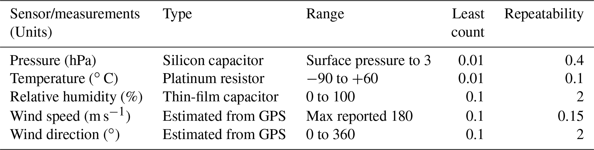
The sondes carry three sensors – one each for measuring pressure (p), temperature (T) and relative humidity (RH), together referred to as the PTU sensors and with a sampling frequency of 2 Hz. The GPS receiver allows the position of the dropsonde to be tracked, from which ambient winds are estimated at a sampling frequency of 4 Hz. The sensors included in the sondes are the same as in Vaisala's RS-41 radiosondes (upsondes), which were also employed during EUREC4A from the BCO and four other ship-based platforms (Stephan et al., 2021). Table 1 provides a brief summary of the type, the resolution and the expected performance from the sensors used in the RD-41 and RS-41 sondes.
2.2 Sonde deployment
A total of 1215 dropsondes were launched: 895 from the German High-Altitude Long Range aircraft (HALO) and 320 from the National Oceanic and Atmospheric Administration (NOAA) Lockheed WP-3D Orion N43-RF aircraft (P3). The P3 was operated as a part of the Atlantic Tradewind Ocean-Atmosphere Mesoscale Interaction Campaign (ATOMIC), which itself was a part of the EUREC4A campaign. Throughout this paper, we use the term EUREC4A to refer to both experiments. More details about HALO's and P3's participation in EUREC4A are provided by Konow et al. (2021) and Pincus et al. (2021), respectively.
Table 2Total number of dropsondes launched, circles flown during the flight, and takeoff and landing times (in UTC, dates in yyyy-mm-dd) for the flight are provided with corresponding flight IDs. Numbers in parentheses in the second column indicate the number of good dropsondes per flight (explained in Sect. 3). Note that the table only shows circles with dropsonde launches. There were also circles flown with no dropsonde launches during EUREC4A.
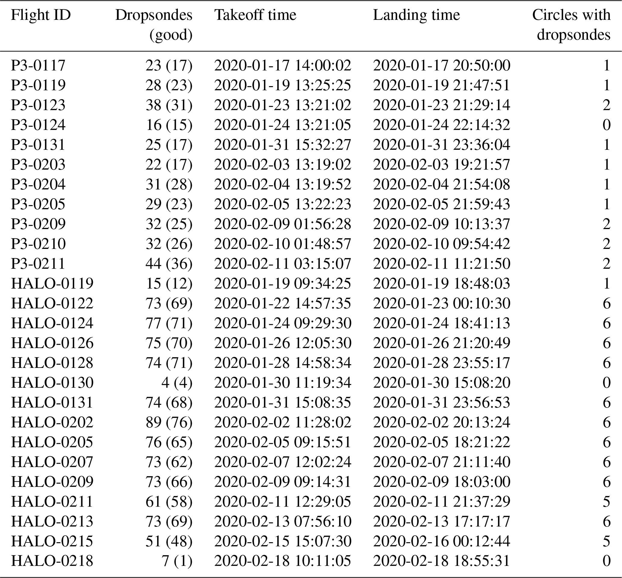
Both aircraft used the Airborne Vertical Atmospheric Profiling System (AVAPS; UCAR/NCAR, 1993) with eight simultaneous channels, for the operation of the dropsondes, as well as for the processing and quality control of collected data. For HALO, the dropsondes are launched from a pneumatic chute controlled manually, which is located at the rear starboard side of the aircraft, slightly oriented towards the bottom of the fuselage. For the P3, the drop point is near the center of the fuselage, with a little offset to the starboard side. HALO typically launched sondes at an altitude between 10–10.5 km, whereas the P3 typically did so at ∼ 7.5 km. Some P3 sondes were launched at ∼ 3 km, when the P3 was flying typical lawn-mower patterns (straight, parallel, long legs connected by shorter, perpendicular legs; parts of some visible in the north in Fig. 1) at low altitudes to facilitate launching airborne expendable bathythermographs (AXBTs). The total number of dropsondes launched from the two aircraft per flight is given in Table 2.
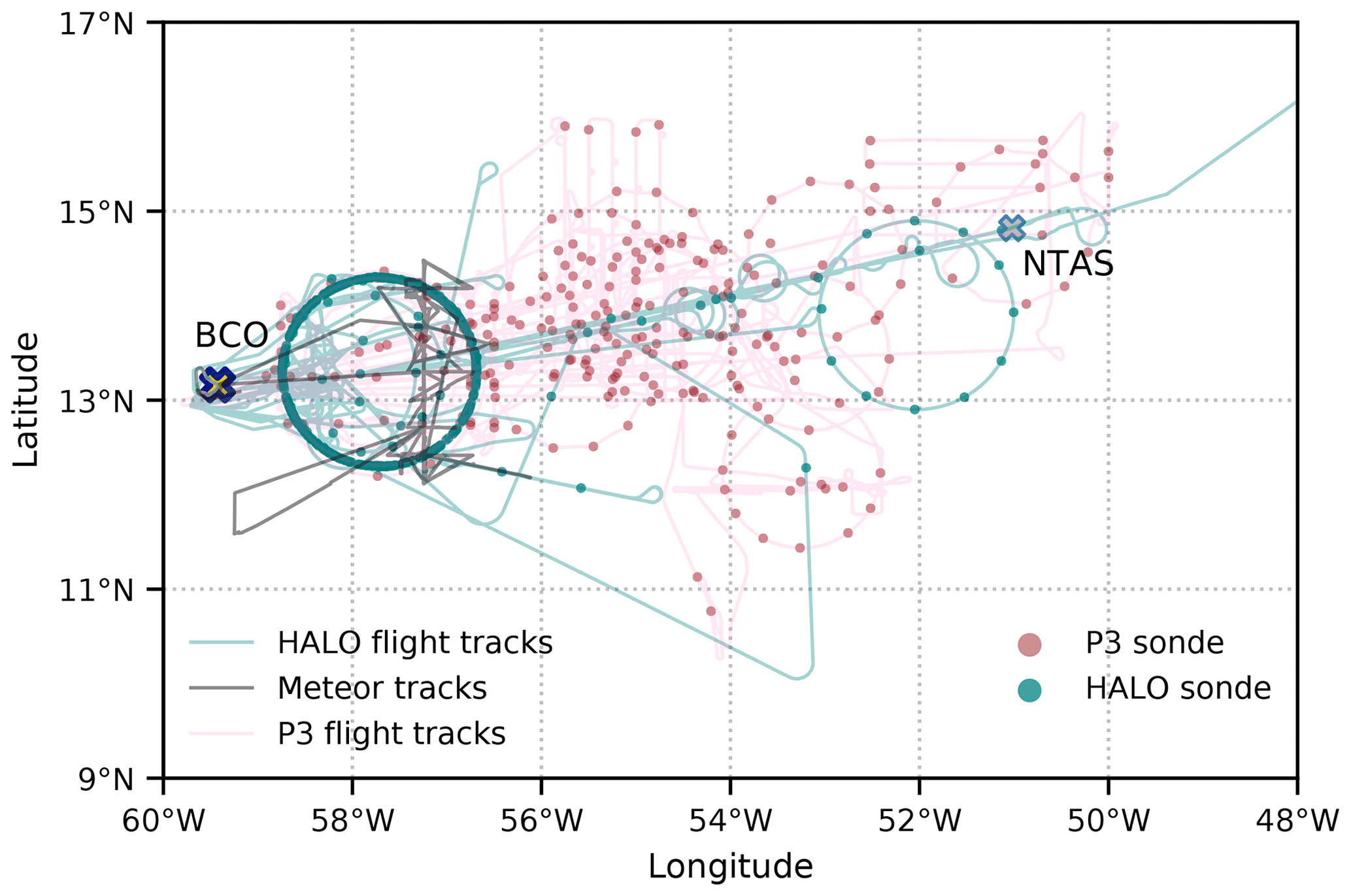
Figure 1Map showing the launch locations of the dropsondes during EUREC4A from HALO (teal) and P3 (red). The flight paths for HALO (light teal), P3 (light pink) and Meteor (gray) are shown as shaded lines. The crosses near the west and east edges of the displayed domain mark the location of the BCO and the NTAS buoy, respectively.
Nearly 90 % (∼ 87 %) of the dropsondes launched reported data as expected, with partial data being recorded by a large percentage of remaining sondes. Only 51 (∼ 4 %) sondes provided no usable data. Almost all of these 51 sondes failed because of an error in automatically detecting launch, the cause for which was later attributed to a manufacturing error in certain batches of dropsondes (Vaisala, personal communication). Success rates for the other aspects of measurements are described in more detail in Sect. 3.
Table 3Details of circles flown during EUREC4A. Circle time (in UTC) is the mean launch time for all sondes in the circle. Longitude (∘ E), latitude (∘ N) and diameter (km) are those associated with the center of a least-squares fitted circle to all sondes. Dropsondes show the total number of sondes launched in each circle. The numbers in parentheses (L4) show the number of good sondes (explained in Sect. 3) used for regression in Level 4.
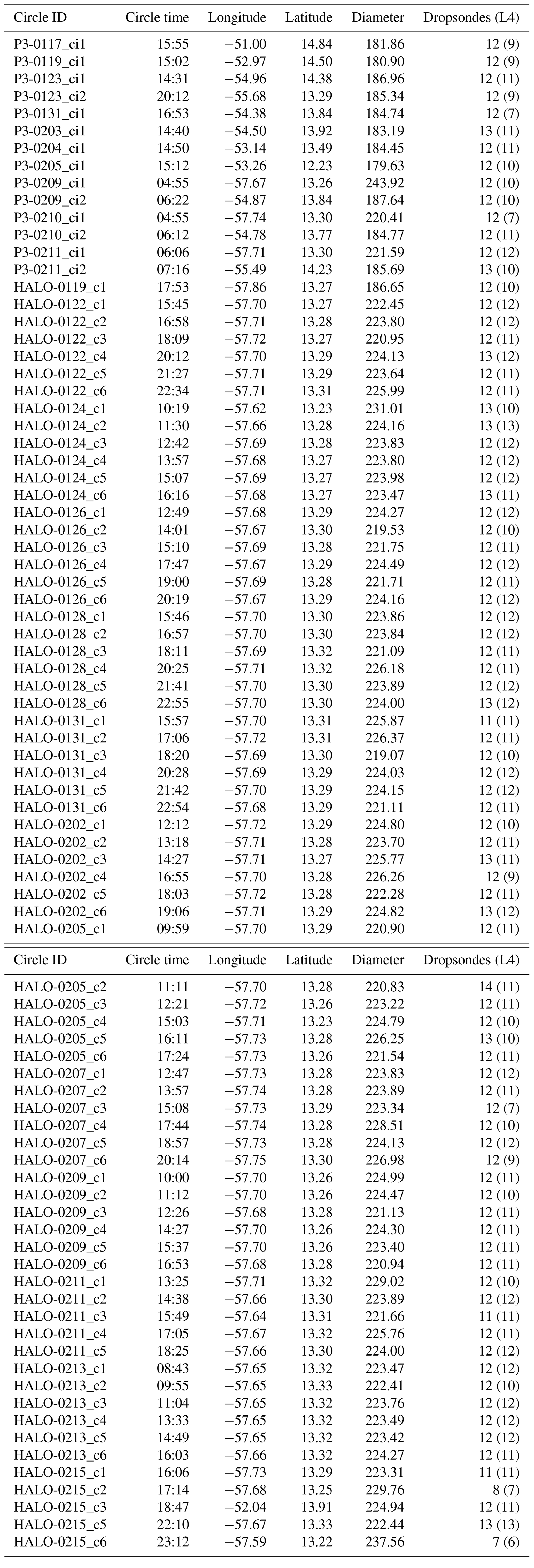
A core part of the EUREC4A campaign was mesoscale circular flight patterns, which were adopted for most (1021 sondes, ∼ 84 %) of the dropsonde launches. The use of a repetitive flight pattern was based on a desire to provide consistent and comparable estimates of meteorological variables. Circles were chosen to facilitate estimates of the profile of the mesoscale (circle) divergence of the horizontal wind. Following the error analysis of Bony and Stevens (2019), each circle aimed to launch 12 sondes. The number of sondes launched per circle is provided in Table 3.
Most circles were flown along a fixed circular path, called the EUREC4A-circle (Stevens et al., 2021), which was planned with the center coordinates as 13.30∘ N, 57.72∘ W and a diameter of roughly 220 km. The location of the sonde launches shown in Fig. 1 highlights the density of HALO sondes concentrated along the circumference of the EUREC4A-circle. This circle was chosen such that complementary measurements are maximized between the aircraft and other platforms in EUREC4A. Measurements performed along the EUREC4A-circle were made irrespective of meteorological conditions and hence were unbiased. Flight times (see Table 2) were adjusted to best sample the diel cycle given operational constraints. HALO was mostly restricted to daylight hours, while the P3 made three flights at night and is the only sampling of the nighttime trades from EUREC4A dropsondes.
The actual mean diameter of all EUREC4A-circles marked by dropsonde launches was 222.82 km, and the mean center was 13.31∘ N, 57.67∘ W. One circuit around the EUREC4A-circle took HALO roughly 60 min to execute at a flight level of about 9.5 km, resulting in sonde launches separated by about 5 min. There were 85 dropsonde circles flown during EUREC4A (see details in Table 3), and 73 of these were EUREC4A-circles, with HALO flying 70 of them and the rest flown by the P3. Of the 12 circles flown which were not EUREC4A-circles, one (HALO-0215_c3) was flown by HALO to provide spatial contrast for comparison with measurements in the EUREC4A-circle. The remaining 11 non-EUREC4A circles were flown by the P3 and were mostly centered on the location of the NOAA research vessel Ronald H. Brown. The flight track of some of the P3 circles was approximated by a dodecagon.
Sondes were also dropped to sample conditions upwind and in the vicinity of EUREC4A-circles, to aid calibration of other instruments, as references for satellite underpasses, and to support surface-based measurements from research vessels and buoys. For instance, HALO typically separated a set of three standard EUREC4A-circles by an upwind “excursion” toward the Northwest Tropical Atlantic Station buoy (NTAS) near 14.82∘ N, 51.02∘ W, along which one to three sondes were launched per flight.
Additional details and strategies for HALO and P3 flights which may be informative for those sondes not launched on standard circles can be found in Konow et al. (2021) and Pincus et al. (2021), respectively.
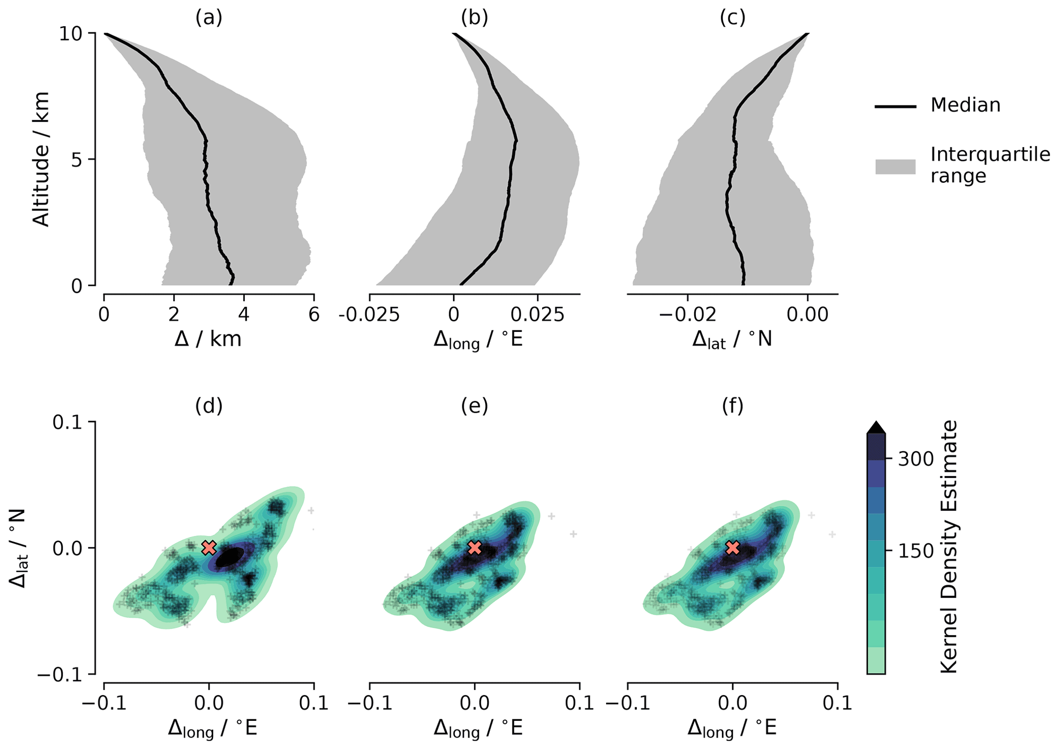
Figure 2An overview of the drift in HALO sondes. Δ indicates horizontal displacement in sondes from launch location. Panels (a)–(c) show the median drift from launch and the corresponding interquartile range for (a) horizontal displacement, (b) longitude and (c) latitude. Panels (d)–(f) show as colors the kernel density estimates (KDEs) of drift from launch location (red cross) at (d) median altitude of maximum drift in the profile, m, (e) at sub-cloud layer mean (0–500 m) and (f) at an altitude of 2 km, where the cloud-top layer is usually present.
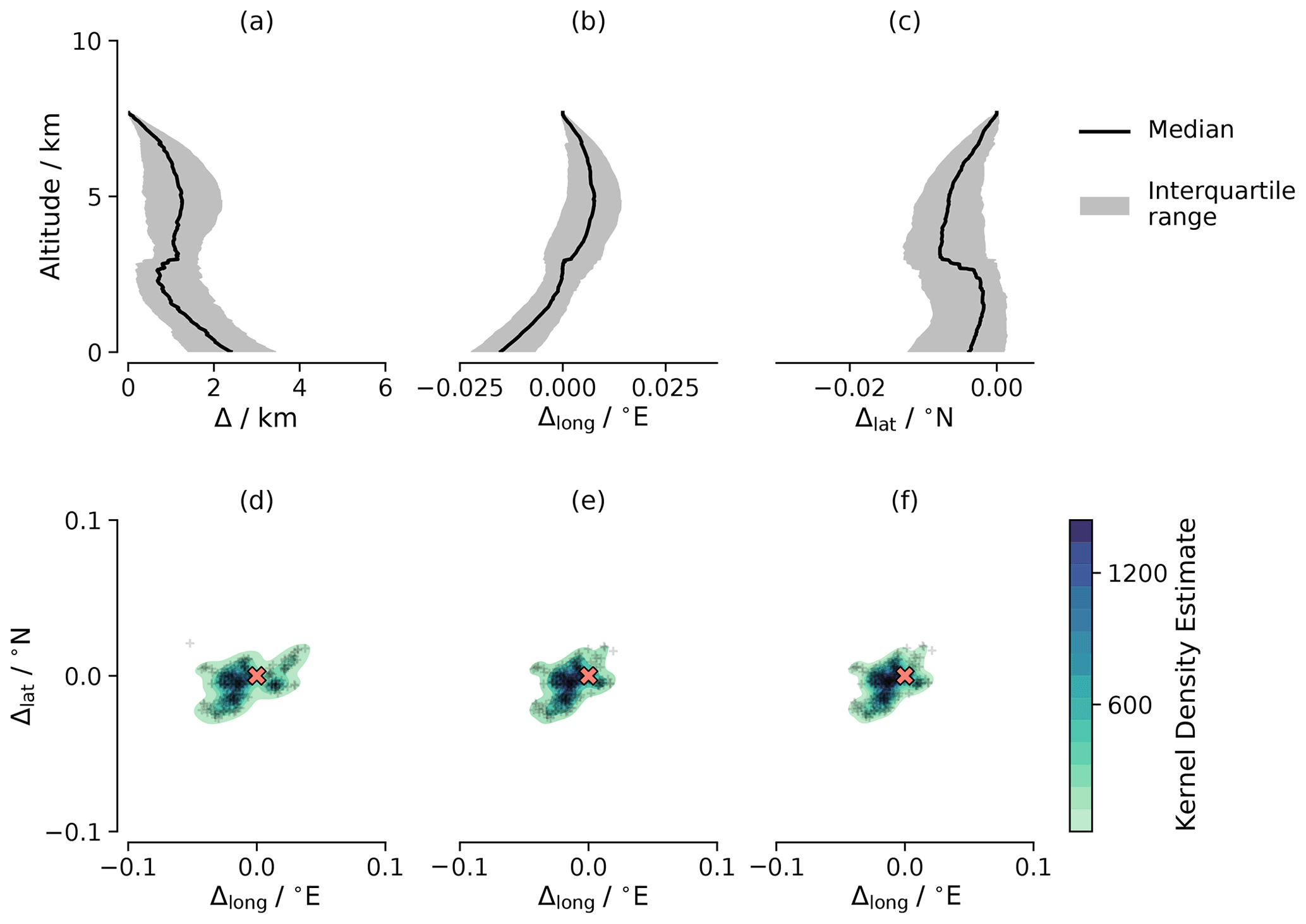
Figure 3Same as Fig. 2, but for P3 sondes instead of HALO sondes. For (d), median altitude of maximum drift in the profile, m.
The maximum drift of the sondes from their launch locations in the horizontal space had a median of around 2.5 km, as seen in Figs. 2 and 3. In the lower troposphere, the drift was generally more along the zonal direction than in the meridional direction, with sondes tending to drift towards the southeast of the launch location. Due to a climatological wind reversal near 3 km, the maximum displacement for HALO is at about this level, whereas for the P3 which dropped its sondes from a lower altitude and thus sampled less of the upper level westerlies, the maximum displacement is at the surface. This also explains why the drift of the P3 sondes is systematically to the west of the drop and less directionally biased for the HALO sondes. The P3 sondes typically sampled the sub-cloud layer ∼ 0.03∘ southwest of the launch location, whereas for HALO sondes, the direction of drift was influenced strongly by the winds above 3 km and therefore varied between different flight days.
2.3 Raw data and initial processing
The raw data collected on the aircraft by AVAPS and the subsequent processing with the Atmospheric Sounding Processing Environment (ASPEN; Martin and Suhr, 2021) software constitute Levels 0 and 1 of JOANNE, respectively. The data included as part of these two levels involve no external adjustments other than the standard processing and quality control by AVAPS and ASPEN – both state-of-the-art tools for dropsonde measurements.
2.3.1 Level 0 (raw data)
Level 0 includes the raw files generated by AVAPS during dropsonde measurements. For every dropsonde launch, multiple files are generated, which store the collected data in different formats, with there being some extent of information overlap between them. These files have names starting with a capitalized letter and are described in Table 4 with the corresponding letter as the file type.
Table 4File types included in Level 0, which are all files in the raw data collected by the dropsondes, and a brief description of what they entail.
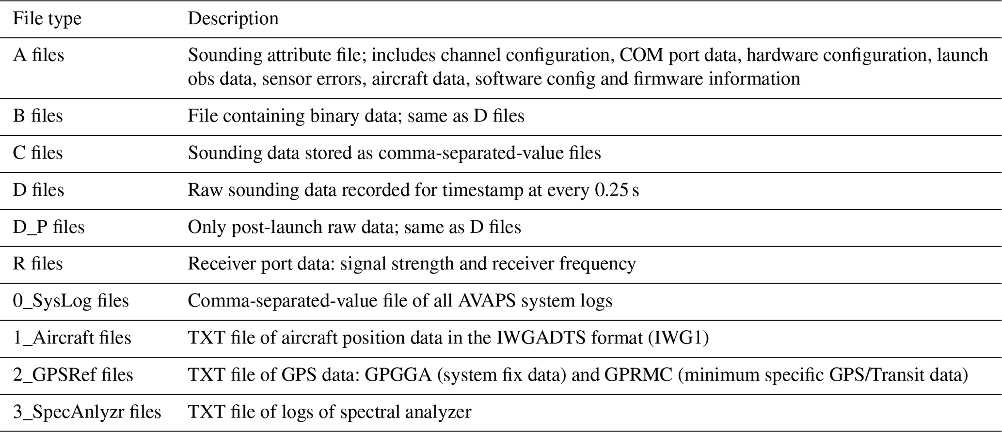
In addition to these files, information about the hardware and the aircraft data is generated and stored each time the AVAPS system is switched on, usually once per flight. These files have names preceded by a number, and the type and content of these files are given in Table 4.
All Level-0 files of a single day (as per UTC) are stored in their respective date directories, with their names in the format YYYYMMDD. The P3 and HALO directories are separated into two different directories named after the respective aircraft.
2.3.2 Level 1 (ASPEN processed data)
Level 1 includes all files from Level 0 after processing by ASPEN. ASPEN takes in D-type files (see Table 4) as input and gives an output of quality controlled files. For JOANNE, the D files were supplied as input to BatchASPEN v3.4.3, and all output files have the suffix _QC. The files are in NetCDF format. For ASPEN processing, we used the standard editsonde configuration. A detailed explanation of the file-structure of these _QC.nc files and the processing steps carried out by ASPEN are outlined in detail by Martin and Suhr (2021). These Level-1 _QC.nc files serve as the input for further processing in JOANNE.
For the data products post Level 1, JOANNE aims to provide sounding profiles that do not contain any obvious measurement errors and contain minimal missing data records. After the ASPEN processing, we run additional QC tests on all Level-1 sounding profiles and filter out soundings that do not meet these objectives. Profiles which are filtered out during this QC are not included in Level 2 and onwards. We believe that soundings passing such a QC stage would best fulfill the purpose of the dropsondes – to characterize the EUREC4A atmospheric environment – with little to no troubleshooting at the user end. However, users who wish to pursue a specific measurement that did not make it past the QC stage can still find it in the exhaustive Level-0 and Level-1 data products.
A sounding's success in the QC stage is provided by a parameter qc_flag, which has possible values of good, bad and ugly. The values stand for fully usable, non-usable and partially usable data, respectively, and are described in more detail later with relevant context. Only soundings flagged as good are included in JOANNE after Level 1. A sounding's qc_flag value is determined by its collective performance in three tests that are designed with the aforementioned QC objectives in mind. These tests are listed as follows.
-
Launch detection test (ld_test). This test filters sondes that failed to detect an automatic launch.
-
Profile fullness test (sat_test). This test filters sondes that did not record measurements for at least 80 % of the time measured in the profile.
-
Low-altitude measurements test (low_test). This test filters sondes whose measurements in the lower levels of the atmosphere do not fall within the expected bounds of parameter values.
The details of how a sounding's performance is judged with these tests and how these tests combine to give the qc_flag value for the sounding are explained further in this section.
3.1 Launch detection test (ld_test)
This test checks whether the sonde detected a launch automatically. If a sonde fails to automatically detect a launch, it does not switch to high-power signal transmission and thus fails to send data back to the AVAPS PC in the aircraft after it has passed further than a short range. The receiver in the aircraft usually failed to detect any signal from such sondes after they had fallen below pressure levels of 300 hPa.
The primary method to check launch detection is to parse through the sounding attribute log files (A type; see Table 4) in Level 0. These files have names starting with “A” and are followed by the date and time of launch. The file extension is the number of the channel used to initialize the sonde and receive its signal. Note that for sondes that did not detect a launch, the file name has time when the sonde was initialized, whereas for the rest, the file name is for the time of the detected launch. The log file contains an internal record termed “Launch Obs Done?”. If this value is 1, the launch was detected; if it is 0, launch was not detected. A sounding’s success in this test is marked by the parameter ld_test and takes values of good or bad, if the corresponding sondes have a successful launch detection or a failed launch detection, respectively. For six sondes, A files were found to be missing in the raw data. These sondes have been tagged as ugly for the ld_test.
3.2 Profile fullness test (sat_test)
This test checks the abundance of measurements within a sounding profile relative to the flight time of the sonde. For a raw measurement profile, time is the independent dimension along which records of measurements are made. The time record is given by the 4 Hz GPS measurements, which means that for the 2 Hz PTU measurements every other record is a missing value. Ideally, all parameters (except u,v) will have measurements at every other time record and u,v at every time record, but in practice, the number of records with measurements always falls short of the ideal number. This is because the time records also include values during initialization as well as during a little before and after the launch, when no signal can be sent back to the AVAPS PC. Thus, the ratio of actual measurements to total possible measurements is lower than the ideal estimate of 1.
The profile fullness test is run by checking the abundance of measurements individually for all parameters in a sounding. The success of the test for a parameter ϕ is recorded in a corresponding parameter ϕ_test, e.g., p_test corresponding to p (pressure), and this success is determined by the ratio of the count of its measurements (n) to its total possible measurements (N), denoted by
Accounting for the different sampling rates of the GPS and PTU measurements, the distributions of ϕsat are shown in Fig. 4, which shows that peaks start to flatten below 0.8. Thus, we set a threshold value of 0.8, and if parameter ϕ has ϕsat lower than this threshold, then it is taken as not having a complete profile, and ϕ_test is flagged as ugly. If ϕsat exceeds or matches the threshold, ϕ_test is flagged as good. If all values are missing, i.e., ϕsat = 0, then ϕ_test is flagged as bad.

Figure 4Kernel density estimate of ratio of actual measurement counts (n) out of maximum possible count of measurements (N), based on the timestamp records in each Level-1 sonde file for (a) HALO and (b) P3. For u, N would be the total timestamp records in any given sonde profile, whereas for the rest it would be half that. In the legend, labels stand for temperature (ta), relative humidity (RH), pressure (p) and eastward wind (u). The northward wind (v) has the same distribution as u and is hence not shown.
Whereas the aforementioned tests (ϕ_test) recorded the success for every parameter in a sounding, we use sat_test to record the success of a sounding. For a given sounding, if all parameter tests are good, the sounding's sat_test is flagged as good. Similarly, if all individual parameter tests are bad, sat_test is flagged as bad. If neither of these conditions is met, sat_test is flagged as ugly.
Figure 4 shows that the abundance of RH values compared to those of pressure (p) and temperature (T) is lower. This is because the RH sensor takes longer to equilibrate to ambient conditions when compared with the other two. This results in fewer measurement records for RH than p and T for the same number of timestamps in the profile.
For HALO’s RH measurements, there were more failures in ASPEN’s Filter Check and Final Smoothing, compared to those for p and T. These checks are part of the post-processing algorithm of ASPEN. The former removes suspect data that deviate by a certain value after the data series is passed through a low-pass filter. As per the standard editsonde configuration that we use, the deviation and the filter wavelength used are 20 % and 20 s, respectively. For the final smoothing, all data (p, T, RH and winds) undergo bspline smoothing with a wavelength of 10 s (Martin and Suhr, 2021).
3.3 Low-altitude measurement test (low_test)
This test functions as a sanity check for the measurements from a sounding in the lower levels of the atmosphere, which is mostly near the surface except for one test where the check is for the lowest 4 km. Similar to the profile fullness test, this test is also determined by the success of parameters over different individual tests. The success of these individual tests is recorded with a parameter name same as that of the corresponding test name. For each of these tests, if the sounding passes the test, it is marked as good, otherwise as bad. The individual tests and their criteria for passing are as follows.
-
low_p_test
This test checks if maximum pressure measured in a sounding is within bounds (1000–1020 hPa), and if so, the sounding passes the test. If the maximum value of p is greater than the upper bound, it is unrealistic, and if it is lesser than the lower bound, it means that the sonde did not measure the near-surface levels of the atmosphere. This test does not check any GPS values. Even if there were no pressure measurements higher than 1000 hPa, there may still be GPS measurements in the low-altitude levels. Such sondes can still be useful for wind and wind-derived products.
-
low_t_test
This test checks if air temperature measured in a sounding is within bounds. It sets two criteria for bounds: (a) maximum air temperature recorded should not be greater than 30 ∘C, and (b) mean T in the bottom 100 m should not be lesser than 20 ∘C. If either of the above limits is violated, measurement of T for the sounding is considered out of bounds and marked as bad. The sonde is also marked bad, if there are no measurements in the bottom 100 m (by GPS altitude (gpsalt) in Level 1).
-
low_rh_test
This test checks if relative humidity measured in a sounding is within bounds. The criterion is that mean RH in the bottom 100 m should not be less than 50 %. If this bound is violated, RH for the sonde is considered out of bounds and marked as bad. The sonde is also marked bad if there are no measurements in the bottom 100 m.
-
low_z_test
This test checks if minimum gpsalt of a sounding is within bounds, i.e., ≤ 30 m above mean sea level. A value higher than the bound means there are no near-surface measurement values of GPS and consequently horizontal winds. This flag does not include any geopotential height values. Even if there are no GPS values below 30 m, there may still be PTU measurements in the lowest levels.
-
palt_gpsalt_rms_test
This test checks if the root mean square (rms) difference between geopotential altitude (palt) and the GPS altitude (gpsalt), for values below 4 km, is lower than 100 m. If the estimated rms difference is below the limit, then the sounding is flagged as good. If the estimated rms difference is greater than the limit, or if there are no values of either palt or gpsalt overlapping in the lower 4 km, then the sounding is flagged as bad. The lack of overlap could be because there are either no palt values or no gpsalt values, or both.
Based on the success in the aforementioned individual tests, the overall success of a sounding for the low-altitude measurement test is recorded in the parameter low_test. If all individual tests are flagged as good, the low_test is flagged as good, and similarly, if all individual tests are flagged as bad, the low_test is flagged as bad. If neither of these conditions is met, the sounding's low_test is flagged as ugly.
Note that the bounds used for the individual tests are all considered keeping in mind the EUREC4A region and conditions. For a similar QC in a different region or environment, the bounds for the parameters will likely be different.
3.4 qc_flag
The overall success of a sounding is recorded as values of good, bad or ugly in the qc_flag parameter and is determined by the combination of success through the three QC tests, as shown in Table 5.
Table 5Determination of qc_flag value based on success of sounding in the three QC tests – ld_test, sat_test and low_test. The asterisk indicates that any value for the test satisfies the condition.

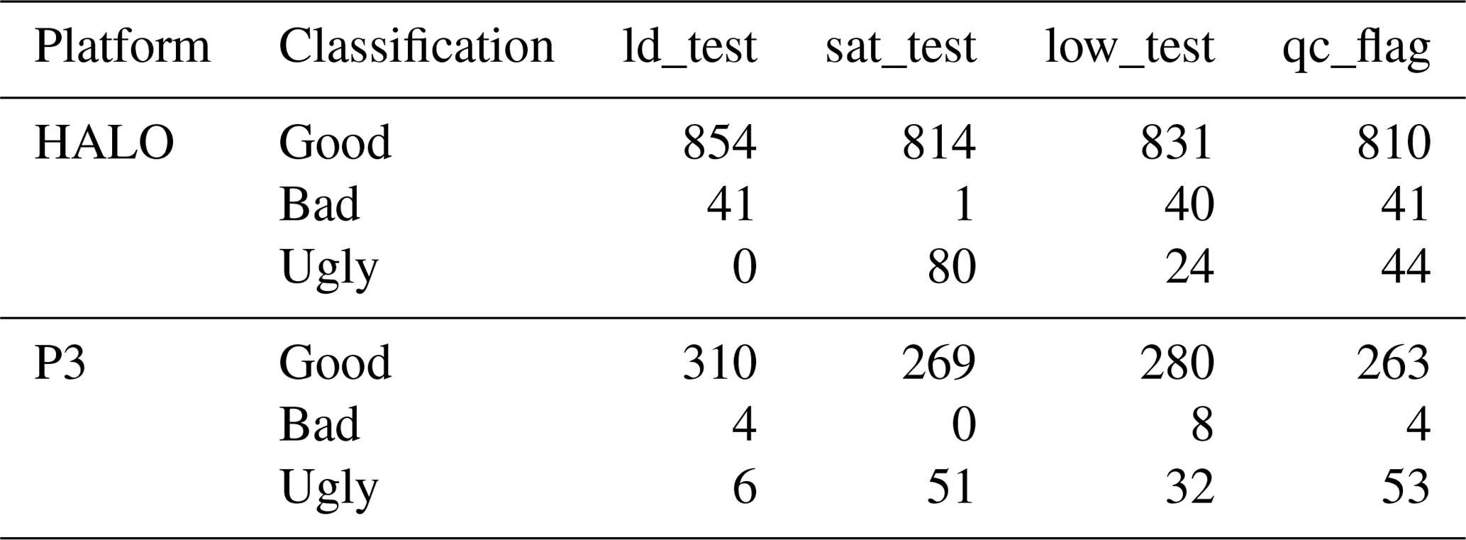
Table 6 summarizes the statistics of the QC tests for HALO and P3. Although the process of classifying the sondes can be simplified by other combinations of the sat_test and low_test values, the method we present ensures no good sondes are omitted, and no bad sondes are admitted. The rest of the sondes, the ugly sondes, still have data that can be salvaged and, after some additional QC, can be combined with the other good sondes depending on the user's objective.
Table 6Count of sondes that passed each QC test, separated by platforms.
JOANNE provides a status file per platform, which stores the results for each individual test and group of tests mentioned above, as well as the final qc_flag classification for each sounding. Thus, the user can still mold the classification based on their objectives and add or remove tests to the process and customize the sonde selection for themselves.
The radiosonde measurements during EUREC4A taken from the BCO and the research vessel Meteor show evidence of a dry bias in the humidity measurements of the HALO dropsondes. The HALO measurements are bounded by Meteor's on the upwind side and BCO's on the downwind side (see Fig. 1). Since all three platforms have unbiased sampling, we expect that the HALO distribution should be between the other two. Figure 5 shows that the BCO and Meteor distributions of RH align closely throughout the lower troposphere, and thus HALO measurements should not differ. The offset in the HALO measurements towards lower RH values suggests a dry bias in the HALO sondes. Since the sensors for the dropsondes and the radiosondes are the same, an instrument difference can be ruled out. Further comparisons with other water vapor measurements in the vicinity such as the radiosondes from the ship Ron Brown, surface humidity measurements from both ships and dropsondes from the P3 aircraft also show HALO's median specific humidity to be lower than expected (not shown).
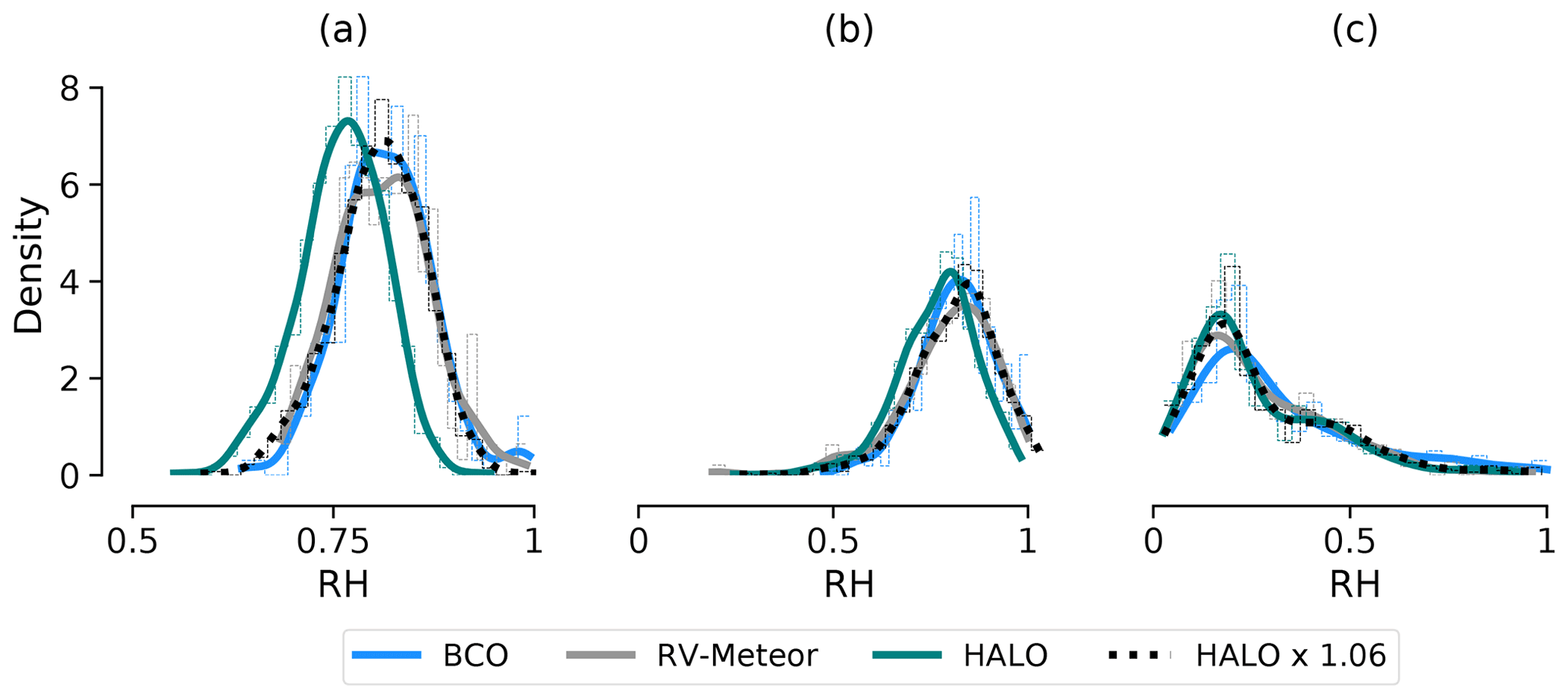
Figure 5Spread (kernel density estimates) in relative humidity values from soundings made by BCO, Meteor and HALO at a (a) mean of 0–500 m, (b) mean of 750–1500 m and (c) mean of 2000–4000 m. The last item in the legend is for RH values of HALO multiplied by 1.06. To coincide with HALO measurement times, BCO and Meteor soundings between 03:00 and 09:00 UTC have been excluded from these distributions, which has a relatively insignificant impact.
A possible contamination of the polymer film in the moisture sensor could affect its dielectric constant, whose fluctuations with respect to relative humidity are subsequently affected. The most plausible explanation is the lack of reconditioning for HALO dropsondes, which resulted in some trace gas pollutants being retained on the humidity sensor and should otherwise have been removed during the reconditioning. The P3 sondes were reconditioned before data collection, and the protocols for P3 and HALO therefore differed in this aspect. This leads us to believe that the dry bias is observed only in HALO dropsondes because of the absent reconditioning. In the case of radiosondes, the reconditioning is part of the automatic calibration process, and so it is not expected to cause problems.
A multiplicative correction factor of 1.06 to the RH values (dotted line in Fig. 5) aligns the HALO distributions well with the BCO and Meteor distributions. The success of this simple rescaling, in matching both the mean and the variance of the distributions, suggests that the bias is both multiplicative and systematic. Had the bias come from a subset of the sondes, a multiplicative correction to match the mean would have resulted in a broader distribution. Had the bias been an additive one, then the correction would have not been as successful at all heights. It is not, however, understood how the contamination of the sensor leads to this dry bias and why the multiplicative correction appears to work so well. However, given the information we have, the multiplicative correction is the best option to correct for the dry bias. Therefore, products from Level 2 onwards include this correction. The values in the rh variable only for the HALO sondes are therefore multiplied by 1.06 when including them in Level 1 from Level 2. All subsequent products in Levels 3 and 4, therefore, have variables derived from the corrected moisture.
Users of the data may note that the correction in HALO dropsonde measurements will propagate into other variables, such as precipitable water (PW), pressure velocity and moisture gradients (since it is apparently multiplicative) and will even have a slight effect on estimates of geopotential altitude which depend on the atmospheric density and hence moisture content. Should the user wish to use the uncorrected moisture values, they can be accessed in Levels 0 and 1.
5.1 Level 2 (quality-controlled sounding data)
The Level-2 NetCDF files contain data from individual soundings, which passed with a qc_flag value of good from the QC stage (discussed in Sect. 3). For Level 2, only variables that are measurements from the dropsonde sensors are included. Redundant state variables are not carried forward from the Level-1 files. Products up to Level 2 maintain the raw measurement profile, and data variables are aligned along the independent dimension time.
File names in Level 1 are generally indicative of launch times; however for sondes that did not detect a launch, the file name indicates time of initialization. The attribute Launch-time-(UTC) in every sounding file of Level 2 should be considered as the final authority on launch time. This is the same as the variable launch_time in Levels 1 and 3.
sonde_id is a variable available in JOANNE products from Level 2 onwards. This is a unique, immutable identifier and is meant to identify exactly one dropsonde which corresponds to exactly one sounding profile. Note that the identifier variable sounding_id in the EUREC4A radiosonde dataset (Stephan et al., 2021) identifies sounding trajectory and not instrument, since one instrument can have upward and downward trajectories. The JOANNE variable sonde_id functions solely as an identifier, and no information should be interpreted from the semantics of this variable.
Table 7Table shows the structure for the Level-2 product, outlining the coordinates and variables and their corresponding descriptions, units and dimensions.
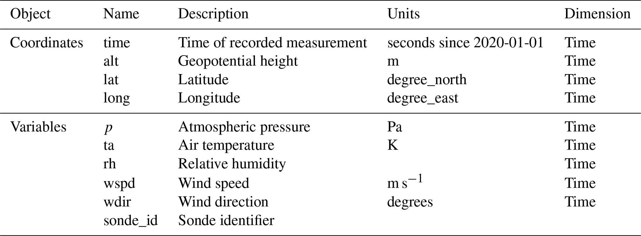
The Level-2 product consists of individual files for every sounding with the file structure as shown in Table 7. All files also include flight information such as position, height and speed as attributes. These are saved by the AVAPS aircraft computer in the sonde A files (see Table 4) and is input from the aircraft system itself. The files also have additional attributes such as the software version for post-processing and quality control. The file names are in the following format:
[campaign]_[project]_[instrument]_[sonde_id]_[version].nc,
e.g., EUREC4A_JOANNE_Dropsonde-RD41_HALO-0124_s42_v0.11.0.nc. Note that sonde_id includes one underscore character within its value for the example shown.
5.2 Level 3 (gridded data)
Level 3 is a product combining dropsonde measurements launched from both the HALO and P3 aircraft, interpolated onto a uniform vertical grid of 10 m spacing, similar to the processing of EUREC4A radiosounding profiles (Stephan et al., 2021). The product is a single file which contains all dropsondes from Level 2 along the altitude dimension alt.
5.2.1 Gridding
The primary objective behind the Level-3 product is gridding all soundings on a common vertical grid, thus making it easier to use the soundings for different analyses. The vertical grid spacing for the dataset is kept at 10 m, up to an altitude of 10 km.
In the case of a regular drop, i.e., if there are no issues like a fast fall, or a failed parachute, the average descent rate of the dropsondes is ∼ 21 m s−1 at 12 km altitude and ∼ 11 m s−1 close to the surface. The PTU sensors have a measurement frequency of 2 Hz, while the GPS has a 4 Hz measurement frequency. This would translate to a vertical sampling of roughly 9–10 m at HALO's flight altitude and 5–6 m close to the surface for the PTU values and correspondingly finer vertical sampling for the GPS-based measurements. Hence the data are slightly coarsened, and only for PTU values in the upper to mid-troposphere do the interpolated values exceed the resolution of the measurements. The gridding is carried out through the following steps.
-
Variables
q(specific humidity),theta(potential temperature),u(eastward wind) andv(northward wind) are computed and added to the dataset (for details, see Sect. 5.2.2). -
All variables along the height coordinate in the dataset are averaged on 10 m bins up to 10 km altitude. In cases where no data are available in the altitude bin, a linear interpolation from neighboring measurements along the height dimension is used to estimate the value in the altitude bin, with the restraint that the neighboring measurements are not further apart than 50 m. If data are not available within 50 m of the desired height level, values at that height level are assigned
_FillValue. While this still allows for a few missing values (∼ 2–3 considering a fall speed of 15–20 m s−1), it does not lead to substantial artificial information created by the smoothened interpolation between points relatively farther away. -
Pressure values are interpolated logarithmically, and these values replace the linearly interpolated pressure values.
-
Temperature (T) and relative humidity (RH) are the originally measured properties by the dropsonde sensors. However, for interpolation q and θ are preferred, as these variables are conserved. After interpolation, T and RH are recomputed from the interpolated values of θ and q. The recomputed values for T and RH replace the previously interpolated T and RH variables from the sounding.
-
Wind speed and wind direction are computed from the interpolated values of u and v and added to the interpolated dataset.
5.2.2 Added variables
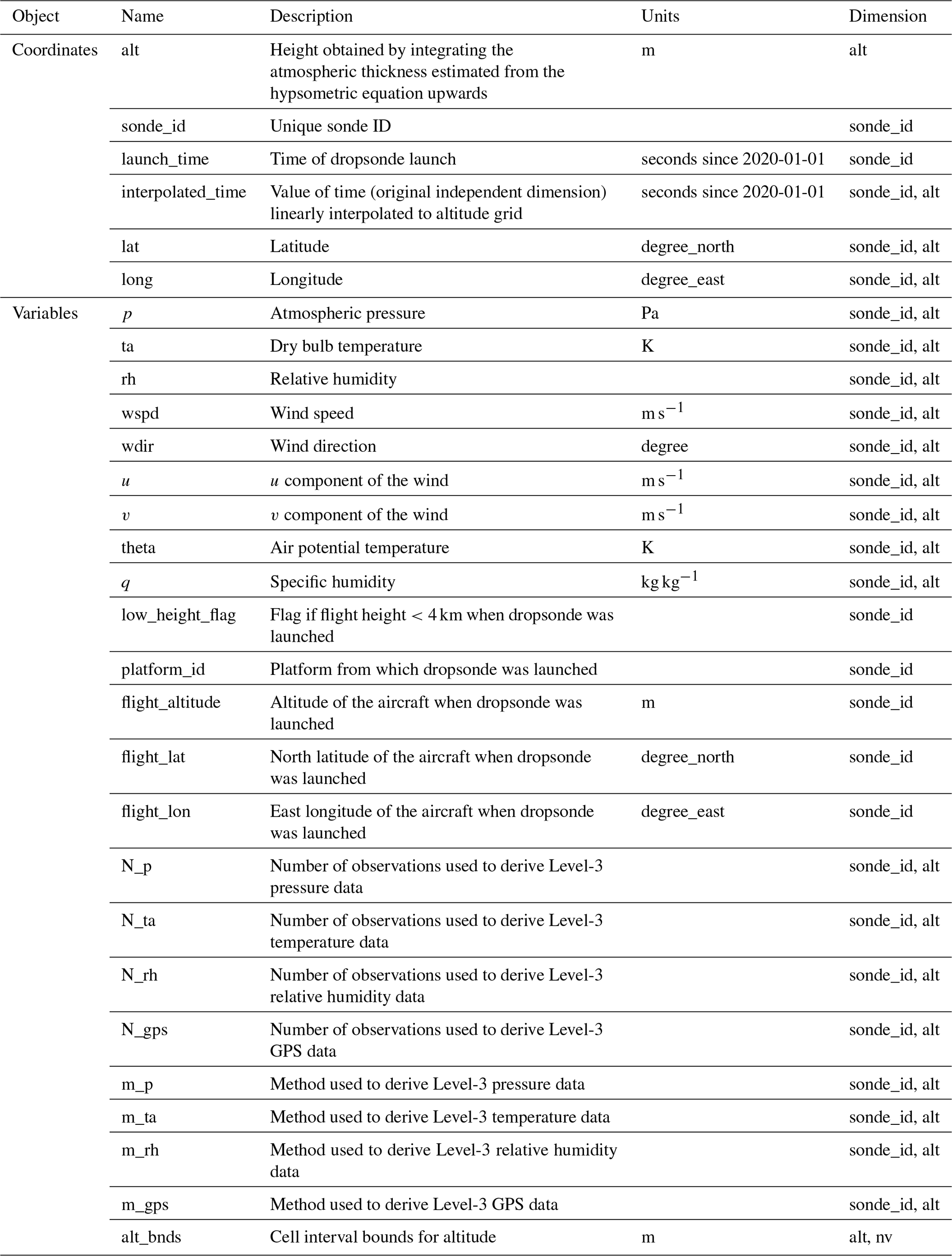
The complete list of variables, their units and their dimensions for Level 3 are provided in Table 8. The descriptions of variables added in Level 3 are as follows.
- Launch time
-
(
launch_time)Level-3 data are of the trajectory type with a single timestamp associated with each sounding, i.e., the launch time. This variable is the same as
launch_timepresent in all Level-1 files. - Potential temperature
-
θ (
theta) and specific humidity q (q)For estimating θ, we consider standard pressure, i.e., 1000 hPa. For the estimation of saturated vapor pressure, the method by Hardy (1998) is used with temperature at every altitude level as input, and subsequently, specific humidity (q) is estimated. The values of θ and q are estimated from the soundings on their respective raw vertical grid before interpolating them on to a common grid.
- Platform name
-
(
platform)Although all soundings are in a single file in Level 3, they can still be separated into HALO and P3 sondes, using this variable, which specifies the platform from which the dropsonde was launched. The values of the variable are strings and have two possible values – “HALO” and “P3”.
- Interpolated time
-
(
interpolated_time)Since time is the independent dimension along which the measurements are made, it is illogical to average or interpolate time along the altitude dimension. Therefore,
timeis not available as a variable from Level 3 onwards. However, for practical purposes, this can be useful information, for instance, to compare with remote-sensing instruments on the aircraft. Thus, relying on the high sampling rate and based on the robust assumption that the dropsondes have negligible upward motion, Level 3 includes the variableinterpolated_time. The variable is computed with linear interpolation, same as for other variables except pressure. - Low flight height flag
-
(
low_height_flag)Some of the sondes from the P3 were launched at an altitude of ∼ 3 km when the aircraft was also launching AXBTs. Therefore, these soundings sampled only the lower levels of the atmosphere, over just half of the depth sampled by other P3 sondes and a third of that of HALO's typical sondes. The
low_height_flagvariable in Level 3 marks sondes that have a launch altitude of less than 4 km, with a value of 1 and otherwise 0. This flag is useful to put in to context estimates of integrated quantities such as total column moisture, as well as to act as an easy separator for users who want to look at profiles in the free troposphere. - Number of measurements in bin
-
(
N_p,N_ta,N_rh,N_gpsand bin method (m_p,m_ta,m_rh,m_gps))The variables
N_p,N_ta,N_rhandN_gpsprovide the number of pressure, temperature, relative humidity and GPS measurements, respectively, in each altitude bin for gridding. Depending on the values of theseNvariables, the corresponding cell methods – denoted by themvariables – are provided. For themvariables, possible values are 0, 1 and 2 and stand for no data, interpolation and averaging, respectively.
Table 8The structure for the Level-3 product, outlining the coordinates and variables and their corresponding descriptions, units and dimensions.
5.3 Level 4 (circle products)
As discussed in Sect. 2.2, the estimation of area-averaged mesoscale properties, such as divergence, was the primary objective behind the sondes' deployment over circular patterns. The Level-4 product provides these circle products as gradient terms estimated by regressing the parameters at each level for a set of sondes comprising a circle. Level 4 also includes terms of divergence, vorticity, vertical velocity and pressure velocity, which are subsequently computed from the gradient terms. The input data are from the gridded dataset in Level 3.
5.3.1 Identifying circles and corresponding sondes
To aid in processing EUREC4A data from aircraft, flight tracks for HALO and P3 were “segmented” into different standard categories such as circles and cloud modules. The flight phase segmentation (FPS) is described in more detail in Konow et al. (2021). We use these FPS files to identify the circles and the dropsondes corresponding to these circle segments. To facilitate ease of working with JOANNE and the FPS files, the circle segments in JOANNE Level 4 have been tagged with the same segment IDs as those in the FPS files. Moreover, the FPS files include a list of dropsondes associated with every flight segment, and this list is comprised of sonde IDs that are the same as that in the JOANNE Level-3 gridded product.
5.3.2 Regression
Following Bony and Stevens (2019), for any parameter ϕ measured by a dropsonde, assuming that variation at any altitude level is linear in horizontal space and is steady in time, the value at any point can be estimated as
where ϕo is the mesoscale mean value, and Δx and Δy are the eastward and northward distances, respectively, from the mean center point of all observed points included in the regression. Minimizing the least-squared errors for the linear regression fit shown in Eq. (2) would give an estimate of the linear variation in the eastward () and northward () directions, along with a value for the intercept for the line (ϕo), providing the mean mesoscale value for ϕ. Formulating this least-squares problem for an overdetermined system of k points as
where and , we solve for x and compute the regression estimates as
where A+ is the Moore–Penrose pseudo-inverse. This pseudo-inverse is obtained from the components of singular value decomposition (SVD) of A. If the SVD of A is written as , then A+ is estimated from the inverse of the SVD components as . Here, U and V are unitary matrices, Σ is a rectangular diagonal matrix with A's singular values and Σ+ is a rectangular diagonal matrix with the reciprocal of A's singular values. We use the linalg.pinv function from the numpy Python library (v1.18.3) to calculate A+.
As a sanity check, we tested the Moore–Penrose pseudo-inverse method of least-squares fitting against the ordinary least-squares fitting by Bony and Stevens (2019), and we found no difference between the solutions (not shown). The advantage with incorporating SVD in the regression is that it significantly reduces computing time, because of the availability of vectorized functions in the numpy library.
The Level-4 product includes the eastward (zonal) and northward (meridional) gradients of temperature, pressure, specific humidity, and u and v winds. Derived from these, Level 4 also provides area-averaged mesoscale divergence (𝒟), vorticity (ζ), vertical velocity (W) and pressure velocity (ω), following Bony and Stevens (2019). The dataset also provides the standard error of each of these regressed estimates as ancillaries to the corresponding variables, thus establishing an extent of confidence in the calculation of these mesoscale properties.
Derived variables in Level 4 are at the same vertical grid of 10 m spacing as in Level 3, and the number of sondes regressed at every level is provided as a variable (sondes_regressed). If at any level, fewer than six sondes have data available, the value for regressed values at that level is set to not a number (NaN). This includes data missing due to no data being recorded as well as sondes removed in any of the previous QC steps. Since the number of sondes regressed change at different levels, this causes abrupt, but generally minor, fluctuations in integrated products such as pressure velocity and vertical velocity.
Table 9The structure for the Level-4 product, outlining the coordinates and variables and their corresponding descriptions, units and dimensions. The ancillary variables (with the prefix “se_”) give the standard error for their corresponding variables indicated by the suffix in the name.
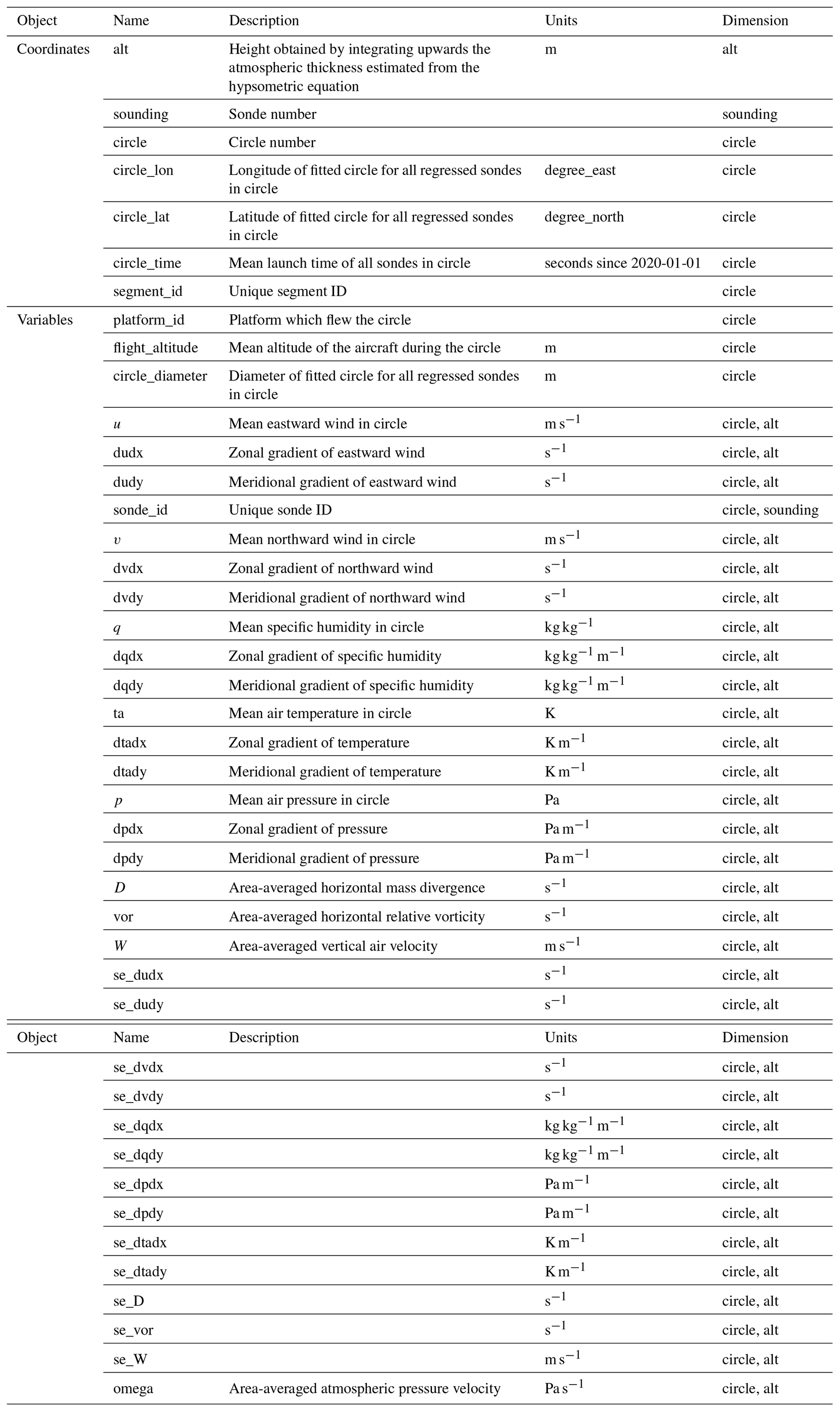
All data variables in Level 4 are along the circle and alt dimensions (see Table 9), and individual sounding data are excluded. The list of sonde IDs included in every circle is included as a variable along dimension sonde_id, making it easier to retrieve data for the individual soundings in the circle.
The JOANNE dataset described in this paper is freely available at AERIS (https://doi.org/10.25326/246, George et al., 2021b). The software used to process the dropsonde data and create JOANNE is also publicly available (https://doi.org/10.5281/zenodo.4746312, George, 2021).
The EUREC4A field campaign took place in January–February 2020 over the North Atlantic trade-wind region. The campaign employed a multitude of platforms measuring a range of atmospheric and oceanographic variables with the objective of understanding shallow clouds and processes that influence them. A core part of the campaign was the deployment of dropsondes to characterize the thermodynamic and dynamic structure of the atmospheric environment. Here, we present JOANNE, the dataset that provides these dropsonde data and additional derived products.
JOANNE presents measurements from 1215 dropsondes launched during EUREC4A by the German research aircraft HALO and the NOAA WP-3D. Dropsondes were primarily released in groups of 12, circumscribing a mesoscale ∼ 222 km diameter circle centered near 13.3∘ N, 57.7∘ W, which we call the EUREC4A-circle. A total of 85 circle patterns were flown with dropsonde launches, 73 being flown by HALO over the EUREC4A-circle along patterns that were not biased toward particular meteorological conditions. In addition, sondes were launched on circular flight patterns centered elsewhere, along lawn-mower flight patterns coinciding with AXBT drops and in a variety of other locations to provide context or calibration for other measurements. Data presented in JOANNE have been quality controlled to eliminate sondes with no, or partially corrupted, data. A total of 51 of the 1215 sondes did not provide usable data, and another 98 provided only partial data and are not included in data products from Level 2 onwards.
A comparison of the HALO dropsondes with radiosondes intensively launched from the R/V Meteor close to the western (upwind) edge of the EUREC4A-circle and with radiosondes launched from the downwind Barbados Cloud Observatory suggests a dry bias. Multiplying relative humidity values by 1.06 appears to largely correct the bias and therefore has been applied from Level 2 onwards to relative humidity and variables derived from it. We found no evidence of such a bias in the P3 sondes, and the reason for the dry bias in HALO seems attributable to a lack of reconditioning of the HALO sondes.
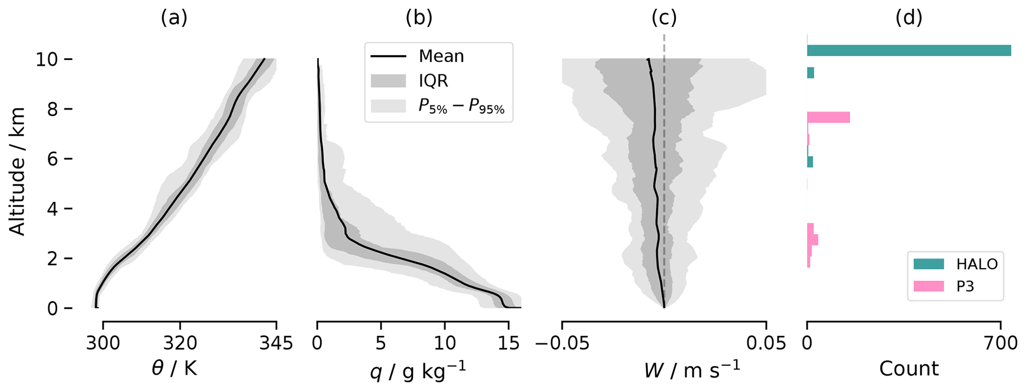
Figure 6Vertical profiles of mean potential temperature (a) and specific humidity (b) from measurements of HALO and P3 sondes. Panel (c) shows the vertical profile of mean vertical velocity from estimates of HALO's EUREC4A-circle measurements. Darkly and lightly shaded regions in (a)–(c) show inter-quartile range (IQR) and 5th–95th percentile range, respectively. Panel (d) shows the histogram for the flight altitude of dropsondes launched from both platforms.
JOANNE is divided into five levels of data products, with increasing order of processing and product retrieval. Level 0 comprises the raw measurement data from the dropsondes collected by AVAPS on the aircraft. Level 1 provides data processed using ASPEN – a state-of-the-art tool for processing raw dropsonde data files. Level 2 consists of individual sounding files that passed through the QC check, but with redundant quantities removed and no derived variables added. Level 3 provides the data after gridding them to a uniform vertical spacing of 10 m, along with derived variables such as potential temperature and specific humidity. Level 4 contains the circle products which are area-averaged and mesoscale variables such as gradients, divergence, vorticity and vertical velocity. Possible sources of uncertainty in JOANNE include sensors' repeatability of measurements (see Table 1), uncertainty from the correction of dry bias in HALO sondes (see Sect. 4) and errors arising from the regression estimates (see Sect. 5.3.2).
JOANNE's immediate usefulness lies in aiding the calibration of or processing the data from remote-sensing instruments on board HALO as well as creation of derived products, e.g., a dataset of radiative profiles from EUREC4A soundings (Albright et al., 2021). Furthermore, the dataset potentially has applications in furthering the understanding of processes in the trades, e.g., the influence of mesoscale circulation on clouds (George et al., 2021a) or the changes in atmospheric properties within a cold pool (Touzé-Peiffer et al., 2021). The vertical profiles and histogram of flight altitude for dropsonde launches shown in Fig. 6 provide an overview for a subset of the atmospheric observations that JOANNE provides. While reaffirming the typical steadiness in the thermodynamic structure of the trades, JOANNE also confirms the high variability in mesoscale vertical motion found by Bony and Stevens (2019) compared to the mean over longer timescales.
JOANNE was conceived by GG. BS and SB designed the sounding strategy for EUREC4A, and RP and CF adapted this for the P3's participation through ATOMIC. HS and TK contributed to the design and processing of the data. GG and BS performed the quality control. The manuscript was mainly written by GG with contributions by BS. GG, HS, MK, HK, MP and JR were responsible for dropsonde launch operations and real-time data quality control over different HALO flights. QTK and AL were responsible for processing and quality-controlling the data for the P3 flights. All authors read and approved the manuscript.
The contact author has declared that neither they nor their co-authors have any competing interests.
Publisher’s note: Copernicus Publications remains neutral with regard to jurisdictional claims in published maps and institutional affiliations.
This article is part of the special issue “Elucidating the role of clouds–circulation coupling in climate: datasets from the 2020 (EUREC4A) field campaign”. It is not associated with a conference.
A great number of people contributed to the launching of the sondes, as recognized in the EUREC4A overview paper. In particular, the authors thank Friedhelm Jansen for his organization and provision of the sondes, Mario Mech and Lutz Hirsch for logistical and technical support, and Angela Gruber for administrative support. Aboard HALO, in addition to the authors, Felix Ament, Jude Charles, Tim Cronin, André Ehrlich, Kerry Emanuel, Florian Ewald, David Farrell, Marvin Forde, Silke Groß, Martin Hagen, Marek Jacob, Theresa Mieslinger, Ann Kristin Naumann, Theresa Lang, Veronica Pörtge, Sabrina Schnitt, Eleni Tetoni, Ludovic Touze-Peiffer, Jessica Vial, Raphaela Vogel, Antone Wiltshire, Allison Wing and Kevin Wolf contributed to the launching of sondes. Akshar Patel launched the sondes from the P3. The authors are also indebted to the ground and flight crews of both aircraft as well as the civil aviation facility and air traffic control for their efforts to facilitate the measurements. Special thanks to Holger Vömel for advice on the possible cause behind the HALO dry bias. GG thanks Anna Lea Albright, Florent Beucher, Xuanyu Chen, Thibaut Dauhut, Geiske de Groot and Louise Nuijens in addition to some names already mentioned for feedback on early versions of the dataset and Ann Kristin Naumann for her comments on the manuscript.
This research was made possible through generous public support provided to, and managed by, the Max Planck Society (DE), DFG HALO SPP 1294 (DE), CNRS (FR) and NOAA (USA). The project also received funding from the European Research Council (ERC) under the European Union's Horizon 2020 research and innovation programme (EUREC4A advanced grant no. 694768) and from the French AERIS research infrastructure.
This paper was edited by Silke Gross and reviewed by two anonymous referees.
Albright, A. L., Fildier, B., Touzé-Peiffer, L., Pincus, R., Vial, J., and Muller, C.: Atmospheric radiative profiles during EUREC4A, Earth Syst. Sci. Data, 13, 617–630, https://doi.org/10.5194/essd-13-617-2021, 2021. a
Bony, S. and Stevens, B.: Measuring Area-Averaged Vertical Motions with Dropsondes, J. Atmos. Sci., 76, 767–783, https://doi.org/10.1175/JAS-D-18-0141.1, 2019. a, b, c, d, e, f
Bony, S., Stevens, B., Ament, F., Bigorre, S., Chazette, P., Crewell, S., Delanoë, J., Emanuel, K., Farrell, D., Flamant, C., Gross, S., Hirsch, L., Karstensen, J., Mayer, B., Nuijens, L., Ruppert, J. H., Sandu, I., Siebesma, P., Speich, S., Szczap, F., Totems, J., Vogel, R., Wendisch, M., and Wirth, M.: EUREC4A: A field campaign to elucidate the couplings between clouds, convection and circulation, Surv. Geophys., 38, 1–40, https://doi.org/10.1007/s10712-017-9428-0, 2017. a
Fleming, J. R.: First woman: Joanne Simpson and the tropical atmosphere, Oxford University Press, https://doi.org/10.1093/oso/9780198862734.001.0001, 2020. a
George, G.: JOANNE (Joint dropsonde Observations of the Atmosphere in tropical North atlaNtic meso-scale Environments) software, Zenodo [code], https://doi.org/10.5281/zenodo.4746312, 2021. a, b
George, G., Stevens, B., Bony, S., Klingebiel, M., and Vogel, R.: Observed impact of meso-scale vertical motion on cloudiness, J. Atmos. Sci., 78, 2413–2427, https://doi.org/10.1175/JAS-D-20-0335.1, 2021a. a
George, G., Stevens, B., Bony, S., Pincus, R., Fairall, C., Schulz, H., Kölling, T., Kalen, Q. T., Klingebiel, M., Konow, H., Lundry, A., Prange, M., and Radtke, J.: JOANNE: Joint dropsonde Observations of the Atmosphere in tropical North atlaNtic meso-scale Environments (v2.0.0), AERIS [data set], https://doi.org/10.25326/246, 2021b. a, b
Hardy, B.: ITS-90 Formulations for Vapor Pressure, Frostpoint Temperature, Dewpoint Temperature, and Enhancement Factors in the Range −100 to +100 C, Proceedings of the Third International Symposium on Humidity and Moisture, April 1998, Teddington, London, UK, 1998. a
Konow, H., Jacob, M., Ament, F., Crewell, S., Ewald, F., Hagen, M., Hirsch, L., Jansen, F., Mech, M., and Stevens, B.: A unified data set of airborne cloud remote sensing using the HALO Microwave Package (HAMP), Earth Syst. Sci. Data, 11, 921–934, https://doi.org/10.5194/essd-11-921-2019, 2019. a, b, c
Konow, H., Ewald, F., George, G., Jacob, M., Klingebiel, M., Kölling, T., Luebke, A. E., Mieslinger, T., Pörtge, V., Radtke, J., Schäfer, M., Schulz, H., Vogel, R., Wirth, M., Bony, S., Crewell, S., Ehrlich, A., Forster, L., Giez, A., Gödde, F., Groß, S., Gutleben, M., Hagen, M., Hirsch, L., Jansen, F., Lang, T., Mayer, B., Mech, M., Prange, M., Schnitt, S., Vial, J., Walbröl, A., Wendisch, M., Wolf, K., Zinner, T., Zöger, M., Ament, F., and Stevens, B.: EUREC4A's HALO, Earth Syst. Sci. Data Discuss. [preprint], https://doi.org/10.5194/essd-2021-193, in review, 2021. a, b, c
Lenschow, D. H., Krummel, P. B., and Siems, S. T.: Measuring Entrainment, Divergence, and Vorticity on the Mesoscale from Aircraft, J. Atmos. Ocean. Tech., 16, 1384–1400, https://doi.org/10.1175/1520-0426(1999)016<1384:MEDAVO>2.0.CO;2, 1999. a
Lenschow, D. H., Savic-Jovcic, V., and Stevens, B.: Divergence and Vorticity from Aircraft Air Motion Measurements, J. Atmos. Ocean. Tech., 24, 2062–2072, https://doi.org/10.1175/2007JTECHA940.1, 2007. a
Martin, C. and Suhr, I.: NCAR/EOL Atmospheric Sounding Processing ENvironment (ASPEN) software, Version 3.4.3, available at: https://www.eol.ucar.edu/content/aspen, last access: 9 November 2021. a, b, c
Pincus, R., Fairall, C. W., Bailey, A., Chen, H., Chuang, P. Y., de Boer, G., Feingold, G., Henze, D., Kalen, Q. T., Kazil, J., Leandro, M., Lundry, A., Moran, K., Naeher, D. A., Noone, D., Patel, A. J., Pezoa, S., PopStefanija, I., Thompson, E. J., Warnecke, J., and Zuidema, P.: Observations from the NOAA P-3 aircraft during ATOMIC, Earth Syst. Sci. Data, 13, 3281–3296, https://doi.org/10.5194/essd-13-3281-2021, 2021. a, b
Stephan, C. C., Schnitt, S., Schulz, H., Bellenger, H., de Szoeke, S. P., Acquistapace, C., Baier, K., Dauhut, T., Laxenaire, R., Morfa-Avalos, Y., Person, R., Quiñones Meléndez, E., Bagheri, G., Böck, T., Daley, A., Güttler, J., Helfer, K. C., Los, S. A., Neuberger, A., Röttenbacher, J., Raeke, A., Ringel, M., Ritschel, M., Sadoulet, P., Schirmacher, I., Stolla, M. K., Wright, E., Charpentier, B., Doerenbecher, A., Wilson, R., Jansen, F., Kinne, S., Reverdin, G., Speich, S., Bony, S., and Stevens, B.: Ship- and island-based atmospheric soundings from the 2020 EUREC4A field campaign, Earth Syst. Sci. Data, 13, 491–514, https://doi.org/10.5194/essd-13-491-2021, 2021. a, b, c
Stevens, B., Farrell, D., Hirsch, L., Jansen, F., Nuijens, L., Serikov, I., Brügmann, B., Forde, M., Linne, H., Lonitz, K., and Prospero, J. M.: The barbados cloud observatory: anchoring investigations of clouds and circulation on the edge of the ITCZ, B. Am. Meteorol. Soc., 97, 787–801, https://doi.org/10.1175/BAMS-D-14-00247.1, 2016. a
Stevens, B., Brogniez, H., Kiemle, C., Lacour, J.-L., Crevoisier, C., and Kiliani, J.: Structure and dynamical influence of water vapor in the lower tropical troposphere, Surv. Geophys., 38, 1–27, https://doi.org/10.1007/s10712-017-9420-8, 2017. a
Stevens, B., Bony, S., Farrell, D., Ament, F., Blyth, A., Fairall, C., Karstensen, J., Quinn, P. K., Speich, S., Acquistapace, C., Aemisegger, F., Albright, A. L., Bellenger, H., Bodenschatz, E., Caesar, K.-A., Chewitt-Lucas, R., de Boer, G., Delanoë, J., Denby, L., Ewald, F., Fildier, B., Forde, M., George, G., Gross, S., Hagen, M., Hausold, A., Heywood, K. J., Hirsch, L., Jacob, M., Jansen, F., Kinne, S., Klocke, D., Kölling, T., Konow, H., Lothon, M., Mohr, W., Naumann, A. K., Nuijens, L., Olivier, L., Pincus, R., Pöhlker, M., Reverdin, G., Roberts, G., Schnitt, S., Schulz, H., Siebesma, A. P., Stephan, C. C., Sullivan, P., Touzé-Peiffer, L., Vial, J., Vogel, R., Zuidema, P., Alexander, N., Alves, L., Arixi, S., Asmath, H., Bagheri, G., Baier, K., Bailey, A., Baranowski, D., Baron, A., Barrau, S., Barrett, P. A., Batier, F., Behrendt, A., Bendinger, A., Beucher, F., Bigorre, S., Blades, E., Blossey, P., Bock, O., Böing, S., Bosser, P., Bourras, D., Bouruet-Aubertot, P., Bower, K., Branellec, P., Branger, H., Brennek, M., Brewer, A., Brilouet , P.-E., Brügmann, B., Buehler, S. A., Burke, E., Burton, R., Calmer, R., Canonici, J.-C., Carton, X., Cato Jr., G., Charles, J. A., Chazette, P., Chen, Y., Chilinski, M. T., Choularton, T., Chuang, P., Clarke, S., Coe, H., Cornet, C., Coutris, P., Couvreux, F., Crewell, S., Cronin, T., Cui, Z., Cuypers, Y., Daley, A., Damerell, G. M., Dauhut, T., Deneke, H., Desbios, J.-P., Dörner, S., Donner, S., Douet, V., Drushka, K., Dütsch, M., Ehrlich, A., Emanuel, K., Emmanouilidis, A., Etienne, J.-C., Etienne-Leblanc, S., Faure, G., Feingold, G., Ferrero, L., Fix, A., Flamant, C., Flatau, P. J., Foltz, G. R., Forster, L., Furtuna, I., Gadian, A., Galewsky, J., Gallagher, M., Gallimore, P., Gaston, C., Gentemann, C., Geyskens, N., Giez, A., Gollop, J., Gouirand, I., Gourbeyre, C., de Graaf, D., de Groot, G. E., Grosz, R., Güttler, J., Gutleben, M., Hall, K., Harris, G., Helfer, K. C., Henze, D., Herbert, C., Holanda, B., Ibanez-Landeta, A., Intrieri, J., Iyer, S., Julien, F., Kalesse, H., Kazil, J., Kellman, A., Kidane, A. T., Kirchner, U., Klingebiel, M., Körner, M., Kremper, L. A., Kretzschmar, J., Krüger, O., Kumala, W., Kurz, A., L'Hégaret, P., Labaste, M., Lachlan-Cope, T., Laing, A., Landschützer, P., Lang, T., Lange, D., Lange, I., Laplace, C., Lavik, G., Laxenaire, R., Le Bihan, C., Leandro, M., Lefevre, N., Lena, M., Lenschow, D., Li, Q., Lloyd, G., Los, S., Losi, N., Lovell, O., Luneau, C., Makuch, P., Malinowski, S., Manta, G., Marinou, E., Marsden, N., Masson, S., Maury, N., Mayer, B., Mayers-Als, M., Mazel, C., McGeary, W., McWilliams, J. C., Mech, M., Mehlmann, M., Meroni, A. N., Mieslinger, T., Minikin, A., Minnett, P., Möller, G., Morfa Avalos, Y., Muller, C., Musat, I., Napoli, A., Neuberger, A., Noisel, C., Noone, D., Nordsiek, F., Nowak, J. L., Oswald, L., Parker, D. J., Peck, C., Person, R., Philippi, M., Plueddemann, A., Pöhlker, C., Pörtge, V., Pöschl, U., Pologne, L., Posyniak, M., Prange, M., Quiñones Meléndez, E., Radtke, J., Ramage, K., Reimann, J., Renault, L., Reus, K., Reyes, A., Ribbe, J., Ringel, M., Ritschel, M., Rocha, C. B., Rochetin, N., Röttenbacher, J., Rollo, C., Royer, H., Sadoulet, P., Saffin, L., Sandiford, S., Sandu, I., Schäfer, M., Schemann, V., Schirmacher, I., Schlenczek, O., Schmidt, J., Schröder, M., Schwarzenboeck, A., Sealy, A., Senff, C. J., Serikov, I., Shohan, S., Siddle, E., Smirnov, A., Späth, F., Spooner, B., Stolla, M. K., Szkółka, W., de Szoeke, S. P., Tarot, S., Tetoni, E., Thompson, E., Thomson, J., Tomassini, L., Totems, J., Ubele, A. A., Villiger, L., von Arx, J., Wagner, T., Walther, A., Webber, B., Wendisch, M., Whitehall, S., Wiltshire, A., Wing, A. A., Wirth, M., Wiskandt, J., Wolf, K., Worbes, L., Wright, E., Wulfmeyer, V., Young, S., Zhang, C., Zhang, D., Ziemen, F., Zinner, T., and Zöger, M.: EUREC4A, Earth Syst. Sci. Data, 13, 4067–4119, https://doi.org/10.5194/essd-13-4067-2021, 2021. a, b
Touzé-Peiffer, L., Vogel, R., and Rochetin, N.: Detecting cold pools from soundings during EUREC4A, EGU General Assembly 2021, online, 19–30 April 2021, EGU21-1038, https://doi.org/10.5194/egusphere-egu21-1038, 2021. a
UCAR/NCAR – Earth Observing Laboratory: NCAR Airborne Vertical Atmospheric Profiling System (AVAPS), UCAR/NCAR – Earth Observing Laboratory, https://doi.org/10.5065/d66w9848, 1993. a
Vaisala: Vaisala Radiosonde RD41 datasheet in English, B211706EN-B, Tech. rep., Vaisala, available at: https://www.vaisala.com/sites/default/files/documents/RD41-Datasheet-B211706EN.pdf (last access: 9 November 2021), 2020a. a, b
Vaisala: Vaisala Radiosonde RS41G datasheet in English, B211321EN-K, Tech. rep., Vaisala, available at: https://www.vaisala.com/sites/default/files/documents/RS41-SG-Datasheet-B211321EN.pdf (last access: 9 November 2021), 2020b. a
Vömel, H., Goodstein, M., Tudor, L., Witte, J., Fuchs-Stone, Ž., Sentić, S., Raymond, D., Martinez-Claros, J., Juračić, A., Maithel, V., and Whitaker, J. W.: High-resolution in situ observations of atmospheric thermodynamics using dropsondes during the Organization of Tropical East Pacific Convection (OTREC) field campaign, Earth Syst. Sci. Data, 13, 1107–1117, https://doi.org/10.5194/essd-13-1107-2021, 2021. a