the Creative Commons Attribution 4.0 License.
the Creative Commons Attribution 4.0 License.
 | 04 Nov 2021
The OH (3-1) nightglow volume emission rate retrieved from OSIRIS measurements: 2001 to 2015
Chris Z. Roth
Adam E. Bourassa
Douglas A. Degenstein
Kristell Pérot
Ole Martin Christensen
Donal P. Murtagh
The OH airglow has been used to investigate the chemistry and dynamics of the mesosphere and the lower thermosphere (MLT) for a long time. The infrared imager (IRI) aboard the Odin satellite has been recording the night-time 1.53 µm OH (3-1) emission for more than 15 years (2001–2015), and we have recently processed the complete data set. The newly derived data products contain the volume emission rate profiles and the Gaussian-approximated layer height, thickness, peak intensity and zenith intensity, and their corresponding error estimates. In this study, we describe the retrieval steps for these data products. We also provide data screening recommendations. The monthly zonal averages depict the well-known annual oscillation and semi-annual oscillation signatures, which demonstrate the fidelity of the data set (https://doi.org/10.5281/zenodo.4746506, Li et al., 2021). The uniqueness of this Odin IRI OH long-term data set makes it valuable for studying various topics, for instance, the sudden stratospheric warming events in the polar regions and solar cycle influences on the MLT.
- Article
(707 KB) - Full-text XML
- BibTeX
- EndNote


The OH airglow is an important feature that aids us in understanding the thermal, dynamical and chemical variations that occur in the mesosphere and lower thermosphere (MLT) region. The infrared imager (IRI) of Odin-OSIRIS (Optical Spectrograph and InfraRed Imaging System) has been routinely measuring the 1.53 µm OH (3-1) emission since the launch in 2001 (night-time measurements are only available between 2001 and 2015), but this complete data set has only recently been processed. In this study, we describe the retrieval of the volume emission rate (VER) profiles of the OH (3-1) layer, and characterise the layer in terms of peak intensity, peak height, thickness and zenith intensity.
The newly processed OH data set is unique. We can access the vertically resolved information thanks to the limb sounding geometry, which the ground-based OH observations such as those operating within the Network for the Detection of Mesospheric Change (NDMC) cannot provide. However, ground-based measurements have advantages over satellite observations, as they provide data sets with better temporal coverage, both in terms of length and frequency, at a given location. Several other space-borne instruments have also measured the limb profiles of the OH layers, namely the Improved Stratospheric and Mesospheric Sounder (ISAMS), the Global Ozone Monitoring by Occultation of Stars (GOMOS), the Microwave Limb Sounder (MLS), the Sounding of the Atmosphere by Broadband Emission Radiometry (SABER), the WIND Imaging Interferometer (WINDII), the SCanning Imaging Absorption spectroMeter for Atmospheric CHartographY (SCIAMACHY) and the optical spectrograph (OS) of OSIRIS. Thanks to Odin’s near-polar orbit and the imaging technique, the IRI provides excellent coverage over the high latitudes and a high sampling frequency in the along-track direction. Moreover, the surprisingly long lifespan of the mission has made it possible for the IRI instrument to collect a long-term data set which is the major advantage over the aforementioned space-borne observations, except for SABER which is still measuring.
The new IRI OH data set has the potential to provide insights into various important scientific topics. To briefly name a few, the short-term (in hours and days), mid-term (in months and seasons) and long-term (in years and decades) variations in the MLT chemical composition have been of interest to the scientific community for a long time. Small-scale gravity waves are known to be the driving force of thermal and dynamical structure in the MLT (e.g. Fritts and Alexander, 2003). The characterisation and quantification of these waves are essential to the modelling community in order to correctly predict the general behaviour of the region (e.g. Limpasuvan et al., 2016; Ern et al., 2018). The high sampling frequency of IRI is capable of resolving small-scale coherent structures (on the order of 100 km) along track within the OH layer. Short-term anomalies in OH may also be induced by external forces such as solar energetic particles (SEPs) (e.g. Damiani et al., 2010), and Degenstein et al. (2005) demonstrated that the IRI oxygen channel skilfully captured such an event on 28 October 2003. García-Comas et al. (2017) used the SABER measurements to derive an empirical formula in order to predict the emission altitude of the OH layer measured over the Sierra Nevada Observatory in Granada. They found a significant short-term variability caused by overlapping waves at the scale of few hours.
Another application of this data set would be the study of sudden stratospheric warming (SSW) events, particularly those resulting in an elevated stratopause (ES). SSWs are, in general, recognised by the weakening or even reversal of the westerly polar vortex caused by planetary-scale waves. Despite what the name suggests, SSWs are associated with cooling and upwelling in the mesosphere (e.g. Orsolini et al., 2017). Specifically, Tweedy et al. (2013) showed that, during such an event, this led to an enhanced secondary ozone layer on a short-term scale. Several days following the onset of such an even, the recovery phase of an ES SSW is characterised by strong downwelling and warming which causes the episodic intensification of the OH emission observed at a lower altitude and can last for more than a month (mid-term-scale anomalies) (Damiani et al., 2010; Shepherd et al., 2010; Gao et al., 2011; Dyrland et al., 2010). Sheese et al. (2014) briefly showed intense OH (8-3) emission after an ES SSW episode in winter 2008–2009 (their Fig. 7), recorded by the OS of OSIRIS. These ES SSWs have occurred multiple times during the Odin mission, as shown by Pérot and Orsolini (2021), which makes the new IRI OH data set well suited for investigating the thermal, dynamical and chemical couplings during these winters.
The global distribution of the semi-annual oscillation (SAO), annual oscillation (AO) and quasi‐biennial oscillation (QBO) projected by the OH nightglow have been studied by Gao et al. (2010) using SABER, by von Savigny (2015) and Teiser and von Savigny (2017) using SCIAMACHY, by Shepherd et al. (2006) using WINDII, and by Zaragoza et al. (2001) using ISAMS. The temporal and spatial coverage of the IRI OH data set can also be expected to demonstrate similar signatures, as seen in the OS OH nightglow observations (Sheese et al., 2014).
Even longer-term variations that occur in the OH airglow can also be investigated, such as those associated with mesospheric cooling and the possible solar cycle influence. Clemesha et al. (2005) pointed out that we do not yet have a consistent picture of the long-term behaviour in the MLT regions concerning solar activity and possible human activities, noting that various measurement techniques have provided conflicting results. There have been several attempts to characterise the solar influence using space-borne observations of OH emission (e.g. Gao et al., 2010; von Savigny, 2015; Teiser and von Savigny, 2017), but the data series available from those instruments were, at the time, hardly long enough to provide any concrete evidence. The long lifespan of the Odin spacecraft has made the IRI data record longer than the 11-year solar cycle; thus, it may be well suited for such investigations.
The structure of the paper is as follows: Sect. 2 provides a brief description of the Odin IRI instrument; Sect. 3 presents the method employed to derive the data products; the fidelity of the obtained data sets is demonstrated in Sect. 4, by looking at the SAO and AO signatures using the monthly zonal averages; and, finally, conclusions are drawn in Sect. 6
Odin was launched into a polar, Sun-synchronous orbit crossing the Equator at 06:00 and 18:00 LT (local time). The satellite orbits the Earth roughly 15 times per day. OSIRIS, one of the instruments aboard Odin, consists of two optically independent sub-instruments: the optical spectrograph (OS) and infrared imager (IRI) (Llewellyn et al., 2004). The IRI instrument includes three channels operating at 1.530, 1.263 and 1.273 µm respectively (channel 1, 2 and 3 respectively). Each channel contains an InGaAs array detector with 128 pixels aligned vertically with 20 masked pixels at the lower end of the array for dark-current correction. The recently updated calibration routines for the Level 1 limb radiance data are essentially the same for all channels, and they are described in Sect. 2.1 of Li et al. (2020).
Channel 1 of the IRI is designed to record both Rayleigh- and aerosol-scattered sunlight and the OH (3-1) Meinel vibration–rotation band airglow. As the recorded signal is dominated by the former in the day part and the latter in the night part of the orbit, this study concerns only the measurements made during the night, i.e. solar zenith angle (SZA) larger than 90∘ at the tangent point. The optical filter overlap on OH (3-1) emission band modelled using the HITRAN database (Gordon et al., 2017) (spectral interval of 1.45–1.8 µm) is shown in Fig. 1, and the overlap ratio is approximately 0.55 for emission temperatures between 150 and 200 K. The overlap ratio is insensitive to the rotational temperature of the emission (less than 0.2 % change per kelvin); thus, a single value is used through out this work.
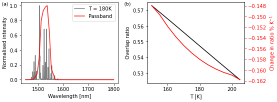
Figure 1(a) The HITRAN-modelled OH (3-1) spectrum at a temperature of 180 K (grey) and the IRI optical passband (red). (b) The overlap ratio (black) of the OH (3-1) emission band (spectral interval of 1.45–1.8 µm) as a function of temperature and its relative change (red).
Figure 2 shows a typical orbit of limb radiance data (referring to the “normal scanning mode” in Odin nomenclature). Due to the nodding motion of the Odin satellite, data plotted in altitude space show data gaps in a “zigzag” pattern. SZA values smaller than 90∘ and/or pixels pointing below 60 or above 95 km tangent are not included in this study, as the signals are not dominated by the OH nightglow under these measurement conditions.
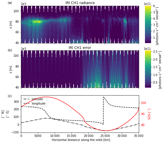
Figure 2(a, b) An orbit of IRI channel 1 limb radiance and its error estimate respectively, recorded in orbit 10122. (c) Latitude (black dot-dashed line) and longitude (black dashed line) coordinate of the image represented tangent point as well as the solar zenith angle (SZA) at that location (red solid line).
The number of orbits that contain at least one vertical limb radiance profile and at least one valid OH nightglow measurement are shown in Fig. 3. The inter-annual variability in the data density is due to the differing operational conditions of Odin over the years. From 2001 to 2007, the observation schedule of Odin was shared equally between a 50 % astronomy mode and a 50 % aeronomy mode. For OSIRIS, this generally meant an arrangement of 3 d of continuous observation and 3 d of rest. From 2008, the astronomy part of the mission ended, and OSIRIS made measurements all day every day for several years; thus, the data density increased. In 2010, the first signs of instrument and satellite ageing started to appear, meaning that 100 % operation could not be maintained. Since then, various on–off patterns have been arranged to maximise the number of measurements obtained while maintaining the health of OSIRIS and Odin as much as possible. Since 2016, OSIRIS can only be operated for a portion of every orbit (less than 50 %, mainly making daytime measurements) due to a power supply unit problem; thus, the OH nightglow measurements are highly limited, particularly after 2018.
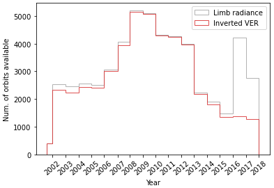
Figure 3Data density from the Odin launch until 2018. The number of orbits that contain at least one limb radiance profile (grey) and that contain at least one OH nightglow profile that is inverted to a volume emission rate (VER) profile (red).
The main focus of this work includes the processing of two data sets, namely the VER of the OH (3-1) nightglow and the airglow layer characteristics in terms of zenith intensity, peak intensity, peak height and layer thickness. This section provides descriptions on how these parameters are derived in steps.
The retrieval of the VER profiles follows the maximum a posteriori (MAP) estimation method (Rodgers, 2000). The principle equation of the inversion is
where xa and Sa are the mean and covariance of the a priori VER respectively, y and Se are the counterparts of the limb radiance measurement, is the inverted VER, and K denotes the weighting functions that represent the linear relationship between the VER and limb radiance.
In this retrieval work, the atmosphere is approximated by a set of 1 km thick homogeneous layers ranging from 55 to 115 km, resulting in a lower margin of 5 km below and a upper margin of 20 km above the limb radiance tangent range (60–95 km). The atmosphere is assumed to be optically thin for the emission, which means that the K matrix is essentially a representation of the path lengths for each line of sight through each atmospheric layer. xa is set to be a zero vector, and Sa is a diagonal matrix with a constant value of (1.1×10⁵)2 for diagonal elements representing altitudes between 60 and 95 km which then exponentially decays to zero for grid points above and below these levels (illustrated by the shading in Fig. 4). These a priori values are used to be pragmatic, as we avoid having to specify a particular vertical distribution for the layer and, thus, complicating the later interpretation. We only regularise the airglow intensity in the form of the uncertainty of the zero a priori profile to allow the inversion scheme to retrieve true to the observed emission with the boundary regions tapered to avoid edge effects.
The covariance of retrieval noise is
Figure 4 depicts the retrieved VER profiles in the form of a 2D histogram of an arbitrary selected series of 200 images. The averaged VER and its error vector (i.e. the square root of the diagonal elements in Sm) of these sample profiles are good representations of a realistic OH airglow profile and its precision respectively. The averaged uncertainty of VER is about 30 % relative to the airglow peak.
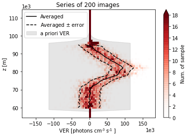
Figure 4Histogram of the volume emission rate (VER) profiles retrieved from the first 200 images taken in orbit 10122 (see Fig. 7 for the whole orbit). Superimposed is the averaged VER (solid line) and ± retrieval noise uncertainty (dashed lines), where the averaging kernel matrix is maximum at rows larger than 0.8 (see Fig. 5). The a priori mean (zero) and uncertainty are illustrated by the grey shading.
The averaging kernel (AVK) matrix
represents the vertical resolution of the retrieved VER profile and maps the changes from the true state x to the estimated state at the corresponding atmospheric grid point. An example of the AVK matrix of a single retrieval is illustrated in Fig. 5. Where there are measurements available, the peak of the AVK is located near the tangent grid point of the corresponding measurement, whereas for those AVKs representing higher altitudes, the peak is close to 95 km. The full width at half maximum of the peaks are 1–1.2 km between 60 and 95 km and rapidly increase to 2.4 km above 95 km, which represents the resolution of the retrieved VER profiles.
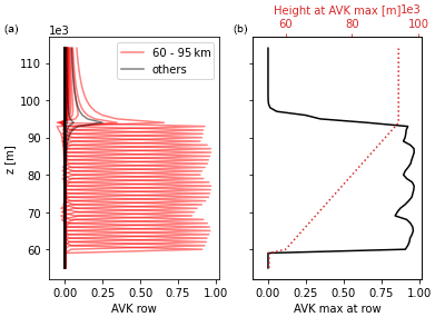
Figure 5The averaging kernel (AVK) matrix of the first volume emission rate (VER) profile taken in orbit 10122 (see Fig. 7 for the whole orbit). (a) Every row of the AVK matrix, with those representing the grid points between 60 and 95 km (red) and those below and above this range (black). (b) The maximum of the AVK matrix in each row (refers to the bottom axis) and the altitude where such a maximum is found (refers to the top axis).
Once the VER profiles are obtained, the next step is to characterise the OH (3-1) emission layer in terms of the zenith intensity, peak intensity, peak height and layer thickness. A Gaussian model serves as a good approximation of the OH layer distribution. As noted by Swenson and Gardner (1998), the modelled Gaussian parameters can be conveniently used for estimating the relative intensity and rotational temperature fluctuations caused by a monochromatic gravity wave. Besides atmospheric wave-induced perturbations, not insignificant random noise is embedded in the signal due to the short integration time of IRI (about 1 s). We make use of the VER random error vector estimated in the previous step to perform a non-linear weighted least squares (WLS) fitting to a Gaussian model:
where the fitted result is the three Gaussian parameters: the airglow peak intensity Vpeak, the peak height zpeak and the full width at half maximum (FWHM) layer thickness , along with their variances and co-variances. Only those VER values associated with a peak AVK value larger than 0.8 are taken as valid (see Sect. 3.1). VER profiles with less than 10 valid grid points are then excluded from the Gaussian fitting procedure. An arbitrarily chosen VER profile is plotted along with the fitted Gaussian function in Fig. 6.

Figure 6The fitted Gaussian model (red), the volume emission rate (VER) profile (grey) and the error profile of the VER (blue), which is the first profile taken in orbit 10122 (see Fig. 7 for the whole orbit). Note that only the grid points associated with an averaging kernel (AVK) maximum at a row larger than 0.8 are used for the fitting, i.e. an altitude from 60 to 95 km (refer to Fig. 5). The fitted Gaussian parameters are as follows: , m and m.
The fitted Gaussian parameters can then be used for further analysis. For instance, the integral of the fitted Gaussian function, which is denoted as the zenith intensity of the OH (3-1) layer Vzenith in this study, can be computed as , and its uncertainty follows the error propagation formula
where ezenith, epeak and eσ denote the standard deviations of Vzenith, Vpeak and σ respectively, and epeakeσρ is the covariance between Vpeak and σ.
The night part of the corresponding orbit of the image in Fig. 6 is shown in Fig. 7. The reconstructed Gaussian layer represents the overall morphology of the OH airglow well, except that the asymmetry of the actual airglow layer, i.e. the different vertical gradient at the lower and upper sides of the layer, cannot be reproduced by the Gaussian model. Furthermore, when the airglow appears to have a double-layered structure, the Gaussian model typically represents it as a very thick layer. The non-Gaussian structure of the airglow layer is represented in the error estimation of the peak height and thickness. Toward the right side of the plots, the airglow layer becomes very weak due to the twilight condition (SZA < 96∘), so that the Gaussian fitting finds large uncertainties for all parameters in that region. Where the airglow structure is prominent, the relative error in Vpeak, zpeak, and Vzenith are less than 25 %, 2 %, 35 % and 60 % respectively for this particular orbit.
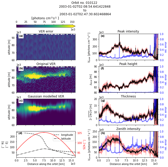
Figure 7The data products resulting from orbit 10122: (a) the retrieved volume emission rate (VER) error, (b) the retrieved VER profiles, (c) the Gaussian reconstructed profiles, and (d) the longitude (black dashed line) and latitude (black dot-dashed line) coordinates of measurements along the orbit as well as the solar zenith angle (SZA; red solid line; right y axis). The modelled Gaussian OH airglow layer (e) peak intensity Vpeak, (f) peak height zpeak, (g) thickness and (h) zenith intensity Vzenith are also shown. The black line corresponds to the expected value, the red shading corresponds to the expected value ± error and the blue line corresponds to the relative error (right y axes).
The possible systematic error sources are summarised in Table 1. The absolute calibration of the radiance is estimated to be the largest source of error, as in-flight calibration capability is lacking. In order to investigate this uncertainty, we used a radiative transfer model (Bourassa et al., 2008; Zawada et al., 2015) to predict the twilight decay of the scattered sunlight signal at lower tangent altitudes, between 30 and 40 km. These conditions are chosen because the upwelling radiation from the Earth surface and clouds is minimised during twilight, and 30–35 km is the upper reach of the stratospheric aerosol layer. Therefore, in these cases, the limb signal is vastly dominated by Rayleigh single scattering and can be reliably predicted. Nevertheless, there is still a large amount of natural variability in the measured signal, making a detailed absolute calibration very difficult to derive; however, we do not observe any systematic changes in the twilight decay of the measured signal when compared to the radiative transfer calculations over a large number of orbits spanning the mission lifetime.
The instrumental pointing is uncertain by 250–500 m (Llewellyn et al., 2004), and this translates to 10 %–15 % based on the OH gradient at the bottom and the upper sides of the layer. A small contribution to systematic error comes from the IRI optical filter shape overlapping the OH (3-1) vibrational transition band, assuming it is temperature insensitive. Moreover, the inversion scheme of VER assumes horizontally homogeneous layer cells. Any inhomogeneity will lead to an additional signal at a lower tangent altitude. In effect, the fitted Gaussian layer will become thicker. The associated systematic error depends on how large and strong the structure is. Note that not all of these errors are relevant for all applications of this data set, and as such, the user needs to reflect on which systematic errors apply to their particular usage.
Table 1A summary of the possible sources of systematic error in the IRI OH VER and their relative errors.
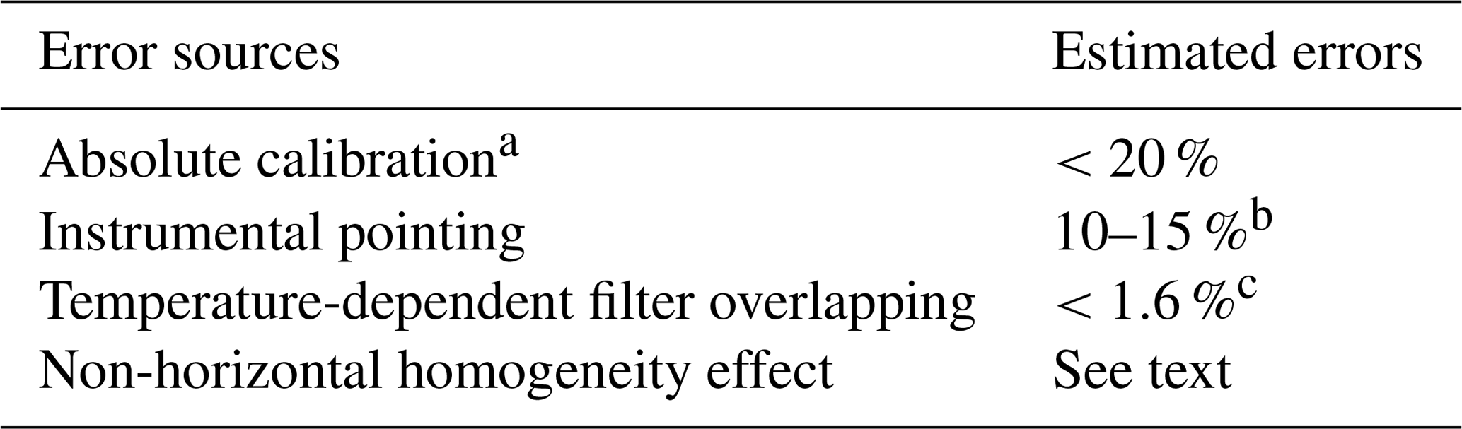
a Due to the lack of an in-flight calibration. b Estimated from 250 to 500 m bias in the pointing uncertainty. c Estimated from a 10 K change around the mesopause.
3.1 Data screening recommendations
To perform meaningful analyses, the data set must be screened as a first step. Because we used arbitrarily chosen prior information about the VER profile, estimated VER grid points with low peak values or a low sum of the rows in the AVK matrix, i.e. low measurement response (MR), should not be included in the analysis. A rule of thumb is that MR values and/or AVK peaks lower than 0.8 should be excluded (Rodgers, 2000), as the retrieved VER is, in such cases, insensitive to the true state (i.e. equal to the zero a priori). This type of screening typically means that the VER profiles are shortened to the altitude grid where measurements exist. The data gaps created are most significant when Odin executes its so-called “mesospheric scan mode”, which is required by other instruments on board. In such cases, the lowest IRI pixel can be as high as 90 km (see Fig. 4 in Li et al., 2020, for reference). We do not perform the Gaussian fitting from a VER profile when the range does not cover at least the 75 to 88 km altitude region.
Another consideration is associated with twilight conditions – at the relevant altitude range this is when the SZA is between 90 and 99.8∘. As the OH (3-1) dayglow intensity is 3 times weaker than its night-time counterpart (Llewellyn et al., 1978), the emission measured under twilight conditions could differ from that during the night. However, if we screen out all measurements that were taken under SZA < 99.8∘ conditions, the majority of the data recorded around the equatorial region year-round as well as at the mid to high latitudes around the equinoxes will be removed. This is a result of the Odin 6–18 h orbit. However, the diurnal variation in OH (3-1) is mainly associated with ozone photodissociation in the Hartley band, which is not significantly affected until the Sun rises above a SZA of 96∘. Therefore, in order to maximise the available data, a lower SZA limit of 96∘ may be used as a screening policy.
Additionally we generally recommend that the user screens particularly noisy profiles. This can be done by either looking at the retrieval error (“error2_retrieval”) or the cost function (“chisq”) of the retrieved profile. The exact filter thresholds used will depend on the application; thus, the end user will need to determine the appropriate value. Similarly, if the Gaussian parameters are used, outliers should be filtered on the total cost of the Gaussian fit (“chisq”).
This section provides a demonstration of the consistency of the new IRI OH data set. The main purpose is to demonstrate the seasonal variability, known from other studies on OH*, such as Shepherd et al. (2006) using WINDII, Gao et al. (2010) and García-Comas et al. (2017) using SABER, Sheese et al. (2014) using OS, and Teiser and von Savigny (2017) using SCIAMACHY. Quantitative and detailed analyses of the characteristics and causes of these variations are beyond the scope of this paper.
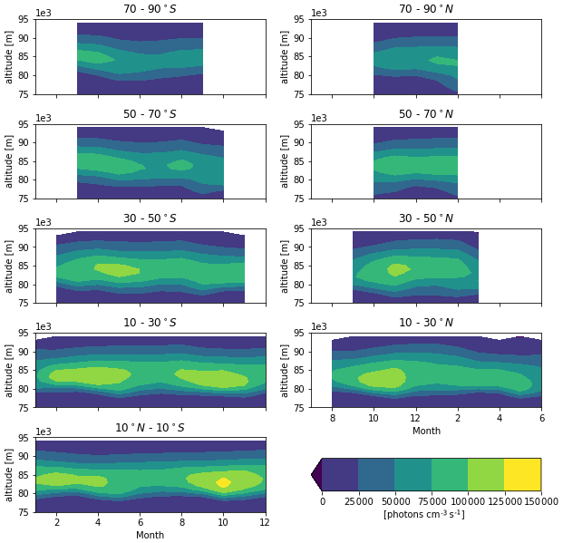
Figure 8Monthly mean zonal average volume emission rate (VER) of all available years. Note that the Northern Hemisphere plots have been shifted by 6 months to ease comparison between the hemispheres.
Figure 8 shows the monthly zonal mean (20∘ latitude bins) of the raw VER profiles for all years where data are available, following the screening policy recommended in Sect. 3.1. Monthly means for each year are computed first and then averaged to a general monthly mean product to prevent the years with higher sampling density from dominating the average. Note that the months in the Northern Hemisphere (NH) are shifted by 6 months in Fig. 8 so that the coloured contours are centred on the plots in order to ease the comparison between the hemispheres. The data cover nearly the whole year between 30∘ N to 30∘ S, and only the winter months at high latitudes.
At mid to low latitudes, the two maxima at the equinoxes are clearly visible and weaken towards the poles, which represents the SAO signature. The two maxima are relatively more symmetric at 10–30∘ S, whereas this is not the case in the equatorial belt and at 10–30∘ N, which is also seen in SABER (Gao et al., 2010) and SCIAMACHY measurements (von Savigny, 2015). In contrast to Shepherd et al. (2006), Gao et al. (2010) and von Savigny (2015), the autumn maximum is stronger than the spring maximum in the NH mid to low latitudes. The airglow is generally brighter in the equatorial region than in the polar regions, which agrees with SABER (Baker et al., 2007) and SCIAMACHY measurements (Teiser and von Savigny, 2017).
At high latitudes above 50∘, the SAO signature weakens. The lack of data in the summer months makes it difficult to provide clear evidence of the AO variation shown in, for example, Gao et al. (2010). The gradient of the bottom side of the airglow layer is less steep (i.e. the layer is more symmetrical around the peak) in comparison to its counterpart at lower latitudes. The hemispheric antisymmetric relationship between the two poles is also visible. In the Southern Hemisphere (SH), the winter airglow begins with a brighter and higher structure, becomes less bright moving to a lower altitude in the middle of winter, and finally moves back to a higher altitude while keeping its weaker brightness at the end of the winter. In the NH winter, the airglow peak altitude is rather flat throughout the season; however, in the early spring, the bottom side becomes extremely thick, which is associated with several episodic SSW events that occurred during the mission. The differences between the two wintertime polar regions are related to the varying strength of the polar vortices.

Figure 9Zonal average monthly running means of the airglow peak intensity (first column), peak height (second column) and layer thickness (third column). Each line represents 1 year of data binned in 20∘ latitude bins (see the top of each panel for labels). Note that the Northern Hemisphere (NH) plots (in red) are shifted by 180 d in order to centre the winter periods to those of the Southern Hemisphere (SH; in blue) and the tropics (in black, bottom row); thus, the horizontal scale is labelled as the SH equivalent (SH-eq.) day of the year (DOY).
Figure 9 depicts the monthly running averages (30 d running window) of the three Gaussian parameters, binned in the same latitude zones as those in Fig. 8 except that we show averages for every year available. Similarly to Fig. 8, the SAO signature is evident in all three parameters, especially at the lower latitudes. The SAO signature in peak height at low latitudes has maxima at solstices (minima at equinoxes), which is also shown by Sheese et al. (2014), Gao et al. (2010), Teiser and von Savigny (2017), and Wüst et al. (2020). Figure 9 also shows the anti-correlation between the peak intensity and peak height, which has been well studied by Liu and Shepherd (2006) and von Savigny et al. (2012), among others. The anti-correlation also exists between the peak intensity and layer thickness, which has been the topic of relatively fewer studies. The hemispheric asymmetry is also visible in the high-latitude bands, as already shown in Fig. 8, as they are closely related to the different characteristics of the two winter polar vortices. Note that discrepancies in observational patterns by the satellite around the North and South poles also exist. The hemispheric asymmetry is also analysed and discussed by Gao et al. (2010), but their focuses were on mid to low latitudes rather than high latitudes (up to 50∘). From Sheese et al. (2014), we can also infer (from their Fig. 5) hemispheric asymmetry at higher latitudes. Several anomalies seen around the North Pole are associated with the episodic SSW events that result in a very intense airglow layer centred at a much lower altitude with a greater thickness, which is depicted in Winick et al. (2009), Damiani et al. (2010), Gao et al. (2011) and Sheese et al. (2014). In general, the variations depicted by these averages of the Gaussian fitted parameters are consistent with the layer characteristics shown in Fig. 8; thus, the data set is self-consistent.
In summary, the IRI OH data set, including the VER profiles and the layer characteristics, is generally consistent with other data sources, although some differences are obviously present. These differences could be due to the local time and other sampling issues, and they would require a detailed study to resolve them.
The IRI OH (3-1) nightglow volume emission rate and its characteristics data sets are publicly available and can be downloaded from the Zenodo data centre: https://doi.org/10.5281/zenodo.4746506 (Li et al., 2021).
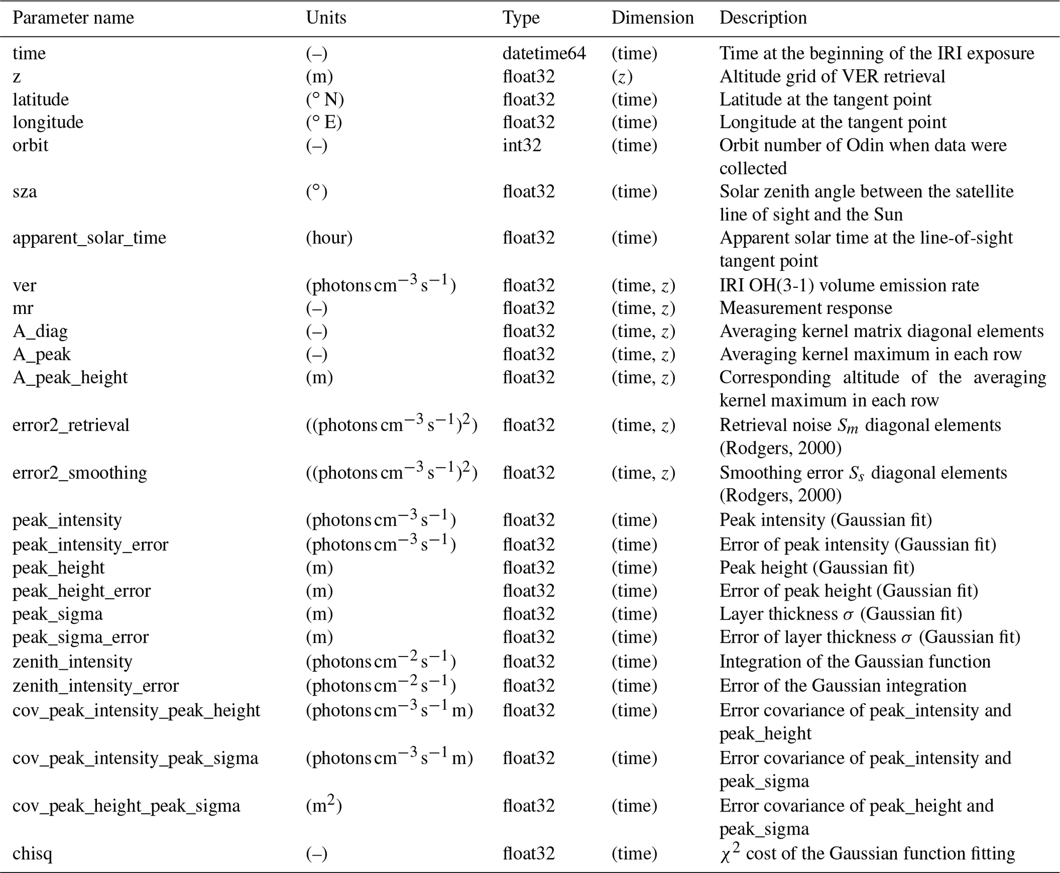
Data sets are structured as 1 year per file in Network Common Data Form (NetCDF) format. File names are in the following format: “iri_ch1_ver_(year).nc”. For example, “iri_ch1_ver_2008.nc” denotes data collected in 2008. The individual parameters included are described in detail in Table 2.
Table 2Parameters included in the “iri_ch1_ver_(year).nc” files, where “(year)” should be replaced by a four-digit number representing the year.
The 15-year data set of the OH (3-1) nightglow measurements collected by the Odin-OSIRIS infrared imager (IRI) has been recently processed. The data set includes two bundles of products: the volume emission rate (VER) profiles and the characteristics of the OH layer in terms of the peak intensity, peak height, layer thickness and zenith intensity. The VER profiles are retrieved by using the maximum a posteriori (MAP) method, assuming horizontally homogeneous atmospheric layer cells. The layer characteristics are assessed by fitting a Gaussian model to the valid VER grid points using the non-linear weighted least squares (WLS) method. All data products contain their error estimations. The recommended data screening policy is described in this paper.
The zonal averages of the data products depict the seasonal variations in the OH layer, consistent with previous studies. These are the well-known semi-annual oscillation (SAO) and annual oscillation (AO) signatures, illustrating the fidelity of the data set. The new IRI OH data set is hereby made available to the scientific community and has good potential for studying several topics in the future, such as the effect of sudden stratospheric warming (SSW) events and solar cycle influences in the mesosphere and the lower thermosphere (MLT) region, owing to the coverage over the high latitudes and the long lifespan of the Odin satellite.
AL prepared all of the calculations and figures. CZR, DAD and AEB (University of Saskatchewan) produced the calibrated IRI data. All authors contributed to the discussions.
The contact author has declared that neither they nor their co-authors have any competing interests.
Publisher’s note: Copernicus Publications remains neutral with regard to jurisdictional claims in published maps and institutional affiliations.
Odin is a Swedish-led satellite project funded jointly by the Swedish National Space Agency (SNSA; grant no. Dnr158/17), the Canadian Space Agency (CSA), the National Technology Agency of Finland (Tekes) and the Centre National d'Etudes Spatiales (CNES) in France. Odin is also part of the ESA's third-party mission programme.
This paper was edited by Nellie Elguindi and reviewed by two anonymous referees.
Baker, D. J., Thurgood, B. K., Harrison, W. K., Mlynczak, M. G., and Russell, J. M.: Equatorial enhancement of the nighttime OH mesospheric infrared airglow, Phys. Scripta, 75, 615–619, https://doi.org/10.1088/0031-8949/75/5/004, 2007. a
Bourassa, A. E., Degenstein, D. A., and Llewellyn, E. J.: SASKTRAN: A spherical geometry radiative transfer code for efficient estimation of limb scattered sunlight, J. Quant. Spectrosc. Ra., 109, 52–73, https://doi.org/10.1016/j.jqsrt.2007.07.007, 2008. a
Clemesha, B., Takahashi, H., Simonich, D., Gobbi, D., and Batista, P.: Experimental evidence for solar cycle and long-term change in the low-latitude MLT region, J. Atmos. Sol.-Terr. Phy., 67, 191–196, https://doi.org/10.1016/j.jastp.2004.07.027, 2005. a
Damiani, A., Storini, M., Santee, M. L., and Wang, S.: Variability of the nighttime OH layer and mesospheric ozone at high latitudes during northern winter: influence of meteorology, Atmos. Chem. Phys., 10, 10291–10303, https://doi.org/10.5194/acp-10-10291-2010, 2010. a, b, c
Degenstein, D. A., Lloyd, N. D., Bourassa, A. E., Gattinger, R. L., and Llewellyn, E. J.: Observations of mesospheric ozone depletion during the October 28, 2003 solar proton event OSIRIS, Geophys. Res. Lett., 32, 1–4, https://doi.org/10.1029/2004GL021521, 2005. a
Dyrland, M. E., Mulligan, F. J., Hall, C. M., Sigernes, F., Tsutsumi, M., and Deehr, C. S.: Response of OH airglow temperatures to neutral air dynamics at 78∘ N, 16∘ E during the anomalous 2003–2004 winter, J. Geophys. Res.-Atmos., 115, D07103, https://doi.org/10.1029/2009JD012726, 2010. a
Ern, M., Trinh, Q. T., Preusse, P., Gille, J. C., Mlynczak, M. G., Russell III, J. M., and Riese, M.: GRACILE: a comprehensive climatology of atmospheric gravity wave parameters based on satellite limb soundings, Earth Syst. Sci. Data, 10, 857–892, https://doi.org/10.5194/essd-10-857-2018, 2018. a
Fritts, D. C. and Alexander, M. J.: Gravity wave dynamics and effects in the middle atmosphere, Rev. Geophys., 41, 1003, https://doi.org/10.1029/2001RG000106, 2003. a
Gao, H., Xu, J., and Wu, Q.: Seasonal and QBO variations in the OH nightglow emission observed by TIMED/SABER, J. Geophys. Res.-Space, 115, A06313, https://doi.org/10.1029/2009JA014641, 2010. a, b, c, d, e, f, g, h
Gao, H., Xu, J., Ward, W., and Smith, A. K.: Temporal evolution of nightglow emission responses to SSW events observed by TIMED/SABER, J. Geophys. Res.-Atmos., 116, D19110, https://doi.org/10.1029/2011JD015936, 2011. a, b
García-Comas, M., López-González, M. J., González-Galindo, F., de la Rosa, J. L., López-Puertas, M., Shepherd, M. G., and Shepherd, G. G.: Mesospheric OH layer altitude at midlatitudes: variability over the Sierra Nevada Observatory in Granada, Spain (37∘ N, 3∘ W), Ann. Geophys., 35, 1151–1164, https://doi.org/10.5194/angeo-35-1151-2017, 2017. a, b
Gordon, I. E., Rothman, L. S., Hill, C., Kochanov, R. V., Tan, Y., Bernath, P. F., Birk, M., Boudon, V., Campargue, A., Chance, K. V., Drouin, B. J., Flaud, J. M., Gamache, R. R., Hodges, J. T., Jacquemart, D., Perevalov, V. I., Perrin, A., Shine, K. P., Smith, M. A., Tennyson, J., Toon, G. C., Tran, H., Tyuterev, V. G., Barbe, A., Császár, A. G., Devi, V. M., Furtenbacher, T., Harrison, J. J., Hartmann, J. M., Jolly, A., Johnson, T. J., Karman, T., Kleiner, I., Kyuberis, A. A., Loos, J., Lyulin, O. M., Massie, S. T., Mikhailenko, S. N., Moazzen-Ahmadi, N., Müller, H. S., Naumenko, O. V., Nikitin, A. V., Polyansky, O. L., Rey, M., Rotger, M., Sharpe, S. W., Sung, K., Starikova, E., Tashkun, S. A., Auwera, J. V., Wagner, G., Wilzewski, J., Wcisło, P., Yu, S., and Zak, E. J.: The HITRAN2016 molecular spectroscopic database, J. Quant. Spectrosc. Ra., 203, 3–69, https://doi.org/10.1016/j.jqsrt.2017.06.038, 2017. a
Li, A., Roth, C. Z., Pérot, K., Christensen, O. M., Bourassa, A., Degenstein, D. A., and Murtagh, D. P.: Retrieval of daytime mesospheric ozone using OSIRIS observations of O2 (a1Δg) emission, Atmos. Meas. Tech., 13, 6215–6236, https://doi.org/10.5194/amt-13-6215-2020, 2020. a, b
Li, A., Roth, C. Z., Pérot, K., Christensen, O. M., Bourassa, A. E., Degenstein, D. A., and Murtagh, D.: OH (3-1) nightglow volume emission rate and its characteristics based on OSIRIS measurements, Zenodo [data set], https://doi.org/10.5281/zenodo.4746506, 2021. a, b
Limpasuvan, V., Orsolini, Y. J., Chandran, A., Garcia, R. R., and Smith, A. K.: On the composite response of the MLT to major sudden stratospheric warming events with elevated stratopause, J. Geophys. Res., 121, 4518–4537, https://doi.org/10.1002/2015JD024401, 2016. a
Liu, G. and Shepherd, G. G.: An empirical model for the altitude of the OH nightglow emission, Geophys. Res. Lett., 33, L09805, https://doi.org/10.1029/2005GL025297, 2006. a
Llewellyn, E. J., Long, B. H., and Soldelm, B. H.: The quenching of OH* in the atmosphere, Planet. Space Sci., 26, 525–231, https://doi.org/10.1016/0032-0633(78)90043-0 1978. a
Llewellyn, E. J., Lloyd, N. D., Degenstein, D. A., Gattinger, R. L., Petelina, S. V., Bourassa, A. E., Wiensz, J. T., Ivanov, E. V., McDade, I. C., Solheim, B. H., McConnell, J. C., Haley, C. S., von Savigny, C., Sioris, C. E., McLinden, C. A., Griffioen, E., Kaminski, J., Evans, W. F. J., Puckrin, E., Strong, K., Wehrle, V., Hum, R. H., Kendall, D. J. W., Matsushita, J., Murtagh, D. P., Brohede, S., Stegman, J., Witt, G., Barnes, G., Payne, W. F., Piché, L., Smith, K., Warshaw, G., Deslauniers, D. L., Marchand, P., Richardson, E. H., King, R. A., Wevers, I., McCreath, W., Kyrölä, E., Oikarinen, L., Leppelmeier, G. W., Auvinen, H., Mégie, G., Hauchecorne, A., Lefèvre, F., de La Nöe, J., Ricaud, P., Frisk, U., Sjoberg, F., von Schéele, F., and Nordh, L.: The OSIRIS instrument on the Odin spacecraft, Can. J. Phys., 82, 411–422, https://doi.org/10.1139/p04-005, 2004. a, b
Orsolini, Y. J., Limpasuvan, V., Pérot, K., Espy, P., Hibbins, R., Lossow, S., Raaholt Larsson, K., and Murtagh, D.: Modelling the descent of nitric oxide during the elevated stratopause event of January 2013, J. Atmos. Sol.-Terr. Phy., 155, 50–61, https://doi.org/10.1016/j.jastp.2017.01.006, 2017. a
Pérot, K. and Orsolini, Y. J.: Impact of the major SSWs of February 2018 and January 2019 on the middle atmospheric nitric oxide abundance, J. Atmos. Sol.-Terr. Phy., 218, 105586, https://doi.org/10.1016/j.jastp.2021.105586, 2021. a
Rodgers, C. D.: Inverse methods for atmospheric sounding : theory and practice., Series on atmospheric, oceanic and planetary physics: 2, World Scientific, 2000. a, b
Sheese, P. E., Llewellyn, E. J., Gattinger, R. L., and Strong, K.: OH meinel band nightglow profiles from OSIRIS observations, J. Geophys. Res., 119, 417–11, https://doi.org/10.1002/2014JD021617, 2014. a, b, c, d, e, f
Shepherd, M. G., Liu, G., and Shepherd, G. G.: Mesospheric semiannual oscillation in temperature and nightglow emission, J. Atmos. Sol.-Terr. Phy., 68, 379–389, https://doi.org/10.1016/j.jastp.2005.02.029, 2006. a, b, c
Shepherd, M. G., Cho, Y. M., Shepherd, G. G., Ward, W., and Drummond, J. R.: Mesospheric temperature and atomic oxygen response during the January 2009 major stratospheric warming, J. Geophys. Res.-Space, 115, A07318, https://doi.org/10.1029/2009JA015172, 2010. a
Swenson, G. R. and Gardner, C. S.: Analytical models for the responses of the mesospheric OH and Na layers to atmospheric gravity waves, J. Geophys. Res.-Atmos., 103, 6271–6294, https://doi.org/10.1029/97JD02985, 1998. a
Teiser, G. and von Savigny, C.: Variability of OH(3-1) and OH(6-2) emission altitude and volume emission rate from 2003 to 2011, J. Atmos. Sol.-Terr. Phy., 161, 28–42, https://doi.org/10.1016/j.jastp.2017.04.010, 2017. a, b, c, d, e
Tweedy, O. V., Limpasuvan, V., Orsolini, Y. J., Smith, A. K., Garcia, R. R., Kinnison, D., Randall, C. E., Kvissel, O. K., Stordal, F., Harvey, V. L., and Chandran, A.: Nighttime secondary ozone layer during major stratospheric sudden warmings in specified-dynamics WACCM, J. Geophys. Res.-Atmos., 118, 8346–8358, https://doi.org/10.1002/jgrd.50651, 2013. a
von Savigny, C.: Variability of OH(3-1) emission altitude from 2003 to 2011: Long-term stability and universality of the emission rate-altitude relationship, J. Atmos. Sol.-Terr. Phy., 127, 120–128, https://doi.org/10.1016/j.jastp.2015.02.001, 2015. a, b, c, d
von Savigny, C., McDade, I. C., Eichmann, K.-U., and Burrows, J. P.: On the dependence of the OH* Meinel emission altitude on vibrational level: SCIAMACHY observations and model simulations, Atmos. Chem. Phys., 12, 8813–8828, https://doi.org/10.5194/acp-12-8813-2012, 2012. a
Winick, J. R., Wintersteiner, P. P., Picard, R. H., Esplin, D., Mlynczak, M. G., Russell, J. M., and Gordley, L. L.: OH layer characteristics during unusual boreal winters of 2004 and 2006, J. Geophys. Res.-Space, 114, A02303, https://doi.org/10.1029/2008JA013688, 2009. a
Wüst, S., Bittner, M., Yee, J.-H., Mlynczak, M. G., and Russell III, J. M.: Variability of the Brunt–Väisälä frequency at the OH*-airglow layer height at low and midlatitudes, Atmos. Meas. Tech., 13, 6067–6093, https://doi.org/10.5194/amt-13-6067-2020, 2020. a
Zaragoza, G., Taylor, F. W., and López-Puertas, M.: Latitudinal and longitudinal behavior of the mesospheric OH nightglow layer as observed by the Improved Stratospheric and Mesospheric Sounder on UARS, J. Geophys. Res.-Atmos., 106, 8027–8033, https://doi.org/10.1029/2000JD900633, 2001. a
Zawada, D. J., Dueck, S. R., Rieger, L. A., Bourassa, A. E., Lloyd, N. D., and Degenstein, D. A.: High-resolution and Monte Carlo additions to the SASKTRAN radiative transfer model, Atmos. Meas. Tech., 8, 2609–2623, https://doi.org/10.5194/amt-8-2609-2015, 2015. a