the Creative Commons Attribution 4.0 License.
the Creative Commons Attribution 4.0 License.
 | 04 Nov 2021
A 1 km global dataset of historical (1979–2013) and future (2020–2100) Köppen–Geiger climate classification and bioclimatic variables
Diyang Cui
Dongdong Wang
Zheng Liu
The Köppen–Geiger classification scheme provides an effective and ecologically meaningful way to characterize climatic conditions and has been widely applied in climate change studies. Significant changes in the Köppen climates have been observed and projected in the last 2 centuries. Current accuracy, temporal coverage and spatial and temporal resolution of historical and future climate classification maps cannot sufficiently fulfill the current needs of climate change research. Comprehensive assessment of climate change impacts requires a more accurate depiction of fine-grained climatic conditions and continuous long-term time coverage. Here, we present a series of improved 1 km Köppen–Geiger climate classification maps for six historical periods in 1979–2013 and four future periods in 2020–2099 under RCP2.6, 4.5, 6.0, and 8.5. The historical maps are derived from multiple downscaled observational datasets, and the future maps are derived from an ensemble of bias-corrected downscaled CMIP5 projections. In addition to climate classification maps, we calculate 12 bioclimatic variables at 1 km resolution, providing detailed descriptions of annual averages, seasonality, and stressful conditions of climates. The new maps offer higher classification accuracy than existing climate map products and demonstrate the ability to capture recent and future projected changes in spatial distributions of climate zones. On regional and continental scales, the new maps show accurate depictions of topographic features and correspond closely with vegetation distributions. We also provide a heuristic application example to detect long-term global-scale area changes of climate zones. This high-resolution dataset of the Köppen–Geiger climate classification and bioclimatic variables can be used in conjunction with species distribution models to promote biodiversity conservation and to analyze and identify recent and future interannual or interdecadal changes in climate zones on a global or regional scale. The dataset referred to as KGClim is publicly available via http://glass.umd.edu/KGClim (Cui et al., 2021d) and can also be downloaded at https://doi.org/10.5281/zenodo.5347837 (Cui et al., 2021c) for historical climate and https://doi.org/10.5281/zenodo.4542076 (Cui et al., 2021b) for future climate.
- Article
(43923 KB) - Full-text XML
-
Supplement
(119 KB) - BibTeX
- EndNote


Climate has direct impacts on the processes and functioning of the ecosystem as well as on the distribution of species (Chen et al., 2011; Ordonez and Williams, 2013; Pinsky et al., 2013; Thuiller et al., 2005). The spatial patterns of climates have often been identified using the Köppen climate classification system (Köppen, 1931).
The Köppen classification system was designed to map the distribution of the world's biomes based on the amplitude and seasonal phase of annual cycles of surface air temperature and precipitation (Köppen, 1936). Compared with other human-expertise-based climate mapping methods (Holdridge, 1947; Thornthwaite, 1931; Walter and Elwood, 1975) and clustering approaches (Netzel and Stepinski, 2016), which suffer from a lack of meteorological basis, the Köppen classification demonstrates stronger correlation with distributions of biomes and soil types (Bockheim et al., 2005; Rohli et al., 2015b). It provides an ecologically relevant and effective method to classify climate conditions by combining seasonal cycles of surface air temperature and precipitation (Cui et al., 2021a).
The Köppen classification has been widely applied in biological science, earth and planetary sciences, and environmental science (Rubel and Kottek, 2011). It is a convenient and integrated tool to identify spatial patterns of climate distributions and to examine relationships between climates and biological systems. It has been found useful for a variety of issues on climate change, such as hydrological cycle studies (Peel et al., 2001; Manabe and Holloway, 1975), Arctic climate change (Feng et al., 2012; Wang and Overland, 2004), and assessment of climate change impacts on ecosystem (Roderfeld et al., 2008), biome distribution (Rohli et al., 2015b; Leemans et al., 1996), and biodiversity (Garcia et al., 2014).
There has been a resurgence in the application of the Köppen climate classification in climate change research over recent decades (Cui et al., 2021a). The Köppen climate classification has been used to set up dynamic global vegetation models (Poulter et al., 2011, 2015), to characterize species composition (Brugger and Rubel, 2013), to model the species range distribution (Tererai and Wood, 2014; Brugger and Rubel, 2013; Webber et al., 2011), and to analyze the species growth behavior (Tarkan and Vilizzi, 2015). The Köppen classification has also been applied to detect the shifts in geographical distributions of climate zones (Belda et al., 2016; Chan and Wu, 2015; Feng et al., 2014; Mahlstein et al., 2013). It also has the potential to aggregate climate information on warmth and precipitation seasonality into ecologically important climate classes, thereby simplifying spatial variability. This climate classification system adds a new direction to develop climate change metrics and can provide support for the growth of species distribution modeling (SDM).
The recent Köppen climate classification maps have a resolution ranging between 0.5∘ and 1 km (Cui et al., 2021a). Early published Köppen climate classification maps have a relatively low resolution of 0.5∘ (Kottek et al., 2006; Grieser et al., 2006a, b; Rubel and Kottek, 2010; Belda et al., 2014; Kriticos et al., 2012). Several map products used interpolation methods to obtain a higher resolution of ∼ 0.1∘ (Peel et al., 2007; Kriticos et al., 2012; Rubel et al., 2017). Fine resolutions of at least 1 km are required to detect microrefugia and promote effective conservation. As the only 1 km global climate classification map product, Beck et al. (2018) provided global climate classification maps for two periods 1980–2016 and 2071–2100 under RCP8.5. The maps were derived using climate data from WorldClim V1 and V2 (Fick and Hijmans, 2017), CHELSA V1.2 (Karger et al., 2017), and CHPclim V1 (Funk et al., 2015). To represent historical climates, they adjusted the inconsistent temporal spans of climatology datasets to the period 1980–2016, by adding interpolated temperature change offsets or multiplying precipitation factors, which may lead to biased coverage of the historical period. Current classification accuracy, temporal coverage, and spatial and temporal resolution of historical and future climate classification maps cannot sufficiently fulfill the current needs of climate change research. Significant changes in the Köppen climates have been observed and projected in the last 2 centuries (Rohli et al., 2015a; Belda et al., 2014; Chen and Chen, 2013; Chan and Wu, 2015; Yoo and Rohli, 2016). Previous studies found that large-scale shifts in climate zones have been observed over more than 5 % of the total land area since the 1980s, and approximately 20.0 % of the total land area is projected to experience climate zone changes under RCP8.5 by 2100 (Cui et al., 2021a). Detection of recent and future changes in climate zones with the application of the Köppen climate maps needs more accurate depiction of fine-grained climatic conditions and continuous and longer temporal coverage.
Table 1Climatology datasets to generate present global maps of the Köppen climate classification with varied spatial resolutions.
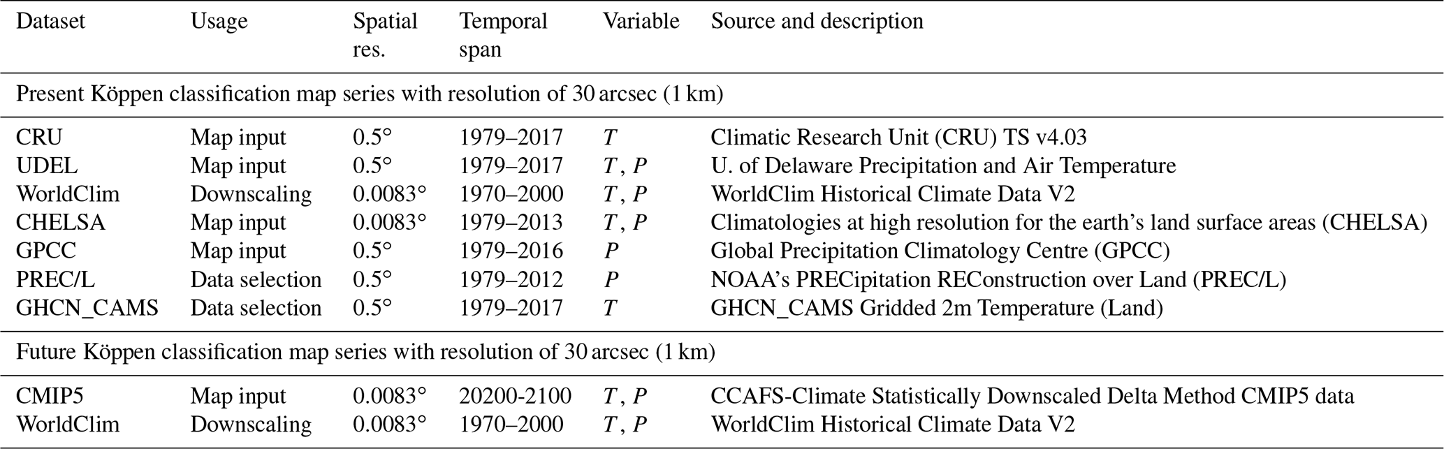
This creates the urgent need for global maps of the Köppen climate classification with increased accuracy and finer spatial and temporal resolutions. Currently available global observational datasets of temperature and precipitation collected during recent centuries and the global climate simulations under alternative future climate scenarios have offered the possibility to create a comprehensive dataset for past and future climates. In this study, we presented an improved long-term Köppen–Geiger climate classification map series for (1) six historical 30-year periods of the observational record (1979–2008, 1980–2009, 1981–2010, 1982–2011, 1983–2012, 1984–2013) and four future 30-year periods (2020–2049, 2040–2069, 2060–2089, 2070–2099) under four RCPs (RCP2.6, 4.5, 6.0, and 8.5). To improve the classification accuracy and achieve a resolution as fine as 1 km (30 arcsec), we combined multiple datasets, including the WorldClim V2 (Fick and Hijmans, 2017), CHELSA V1.2 (Karger et al., 2017), CRU TS v4.03 (New et al., 2000), UDEL (Willmott and Matsuura, 2001), and GPCC datasets (Beck et al., 2005) and bias-corrected downscaled Coupled Model Intercomparison Project Phase 5 (CMIP5) model simulations (Navarro-Racines et al., 2020) (Table 1). We used the WorldClim Historical Climate Data V2 (Fick and Hijmans, 2017) to downscale the 0.5∘ climatology datasets including CRU, UDEL, and GPCC, and we derive high-resolution climate data for the historical periods. To determine the final climate class, we used the climate class with the highest agreement level from an ensemble of climate maps derived from different combinations of surface air temperature and precipitation products, as implemented in Beck et al. (2018). In addition to the Köppen–Geiger climate maps, we also calculated 12 bioclimatic variables at the same 1 km resolution using these climate datasets for the same historical and future periods. This dataset can be used to in conjunction with SDMs to promote biodiversity conservation, or to map plant functional type distributions for Earth system model simulations, or to analyze and identify recent and future changes in climate zones on a global or regional scale.
To validate the Köppen–Geiger climate classification maps, we used the station observations from Global Historical Climatology Network-Daily (GHCN-D) (Menne et al., 2012) and the Global Summary of the Day (GSOD) (National Climatic Data Center et al., 2015) database. At the regional and continental scales, we compared our Köppen–Geiger climate classification maps with previous map products, associated maps of forest cover, and elevation distribution for (1) regions with large spatial gradients in climates, including central and eastern Africa, Europe, and North America, and (2) regions with sharp elevation gradients, including the Tibetan Plateau, central Rocky Mountains, and central Andes. Further, we conducted sensitivity analysis with respect to classification temporal scale, dataset input, and data integration methods. We also provided a heuristic example which used climate classification map series to detect the long-term area changes of climate zones, showing how the Köppen–Geiger climate classification map series can be applied in climate change studies.
Table 1 lists the climatology datasets with global coverage and on a monthly time step, used to generate historical and future Köppen–Geiger climate map series. The present 1 km Köppen–Geiger classification map series for 1979–2013 was derived from the Climatologies at High-resolution for the Earth's Land Surface Areas (CHELSA) V1.2 (Karger et al., 2017), WorldClim Historical Climate Data V2 (Fick and Hijmans, 2017) and statistically downscaled Climatic Research Unit (CRU) TS v4.03 (New et al., 2000), University of Delaware Precipitation and Air Temperature (UDEL) (Willmott and Matsuura, 2001), and Global Precipitation Climatology Centre (GPCC) (Beck et al., 2005) datasets. To decide the datasets to use, we conducted a sensitivity analysis on the input climatology datasets and utilized monthly air temperature datasets from CRU, UDEL, and GHCN_CAMS gridded 2 m temperature (Fan and Dool, 2008) and monthly precipitation datasets from GPCC, UDEL, and NOAA's PRECipitation REConstruction over Land (PREC/L) (Chen et al., 2002). Evaluation results indicated that incorporating only CRU, UDEL temperature datasets, and UDEL, GPCC precipitation datasets and excluding GHCN_CAMS and PREC/L datasets led to higher accuracy in the classification results. Therefore, we chose CRU, UDEL, and GPCC datasets as the classification system input to boost the final accuracy.
To explicitly correct topographic effect, we used 1 km CHELSA V1.2 and WorldClim V2 datasets in addition to the 0.5∘ resolution datasets. The CHELSEA dataset statistically downscaled temperature data from the ERA-Interim climatic reanalysis. For precipitation data, it incorporated multiple orographic predictors and performed bias correction (Karger et al., 2017). With major topo-climatic drivers considered, the CHELSA dataset demonstrated good performance in ecological science studies. CHELSA data exhibited comparable accuracy for temperatures and better predicted precipitation patterns based on the validation results (Karger et al., 2017).
We produced the future Köppen classification map series using the CCAFS statistically bias-corrected and downscaled CMIP5 climate projections (Navarro-Racines et al., 2020). The CCAFS presented a global database of future climates developed by a climate model bias correction method based on the CMIP5 GCM simulations (Taylor et al., 2012) archive, coordinated by the World Climate Research Programme in support of the IPCC Fifth Assessment Report (AR5) (Hartmann et al., 2013). The total is 35 GCMs, and all RCPs, RCP2.6, 4.5, 6.0, and 8.5 (Table S1 in the Supplement). Projections are available at varied coarse scales (70–400 km). To achieve high-resolution (1 km) climate representations, the downscaling method has been applied with the use of the WorldClim data (Fick and Hijmans, 2017). Technical evaluation showed that the bias-correction method that CCAFS data applied reduced climate model bias by 50 %–70 %, which could potentially address the bias issue in model simulations for the threshold-based Köppen classification scheme (Navarro-Racines et al., 2020).
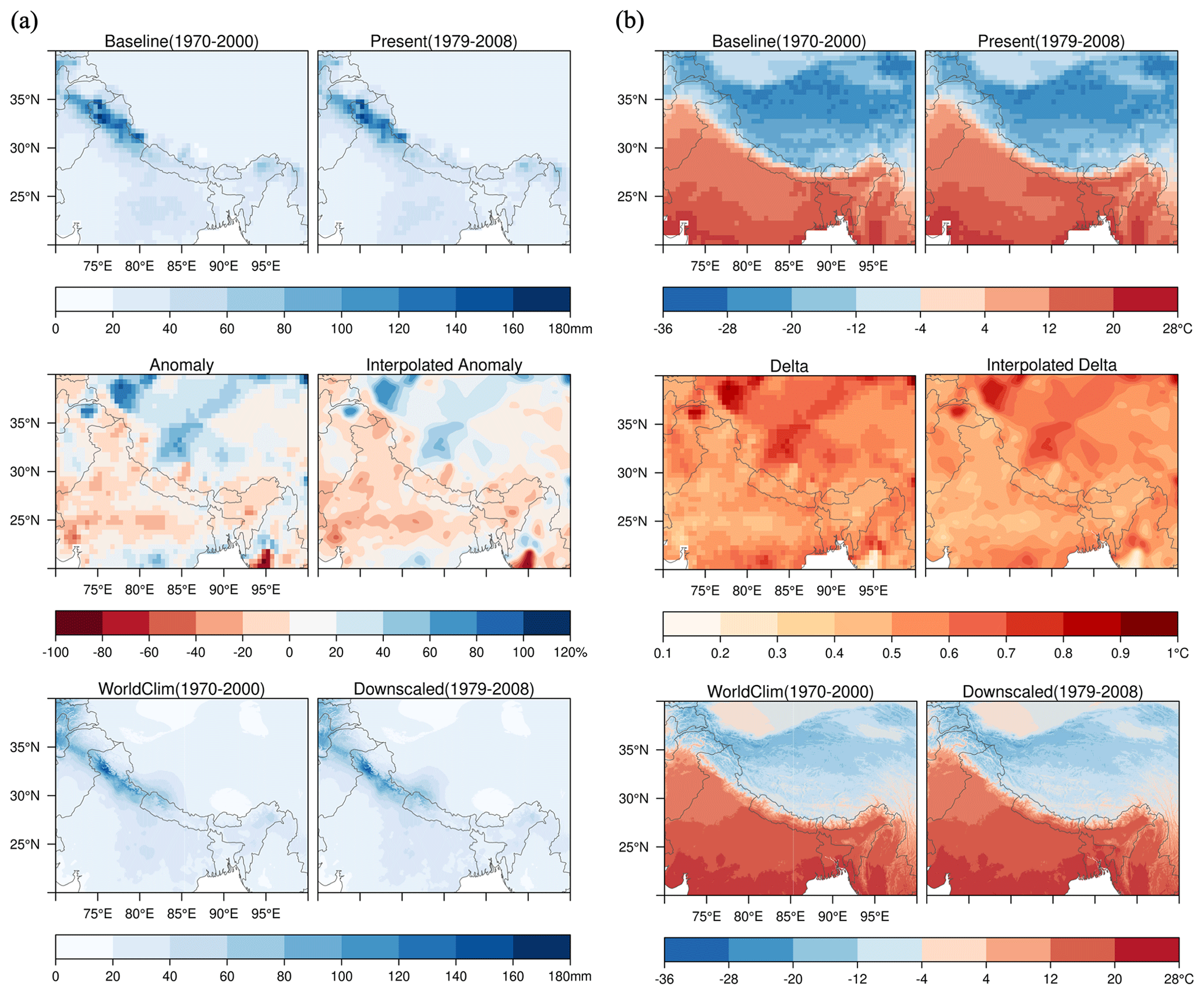
Figure 1Illustration of the downscaling process. (a) Anomaly downscaling method with January total precipitation from GPCC dataset and (b) delta downscaling method with January temperature from CRU dataset. Baseline (1970–2000) and present-day climate data (e.g., 1979–2008) are from CRU, UDEL, or GPCC datasets, which have a coarse spatial resolution of 0.5∘. Precipitation anomaly is change factor of monthly precipitation from baseline to present-day climates. Temperature delta is change in monthly air temperature from baseline to present-day climates. WorldClim (1970–2000) climate data are adjusted by multiplying 30 arcsec interpolated anomaly (for precipitation) or adding 30 arcsec interpolated delta (for temperature) to generate the downscaled climate surfaces with 30 arcsec resolution. Precipitation values are in millimeters per month, and temperature values are in degrees Celsius.
3.1 Köppen–Geiger climate classification
The Köppen climate classification scheme was first introduced by Wladimir Köppen (Köppen, 1936). It is one of the earliest quantitative classification systems of Earth's climates. Its modification, the Köppen–Geiger classification (KGC), was first published in 1936 (Köppen, 1936), developed by Wladimir Köppen and Rudolf Geiger. KGC identifies climates based on their effects on plant growth from the aspects of warmth and aridity and classifies climate into five main climate classes and 30 subtypes (Rubel and Kottek, 2011). The five main climate zones distinguish between plants of the tropical climate zone (A), the arid climate zone (B), the temperate climate zone (C), the boreal climate zone (D), and the polar climate zone (E) (Sanderson, 1999). All main climate zones are thermal zones except the arid (B) climate zone, which is defined based on precipitation threshold.
Table 2Criteria of the Köppen–Geiger climate classification with temperature in degrees Celsius and precipitation in millimeters.
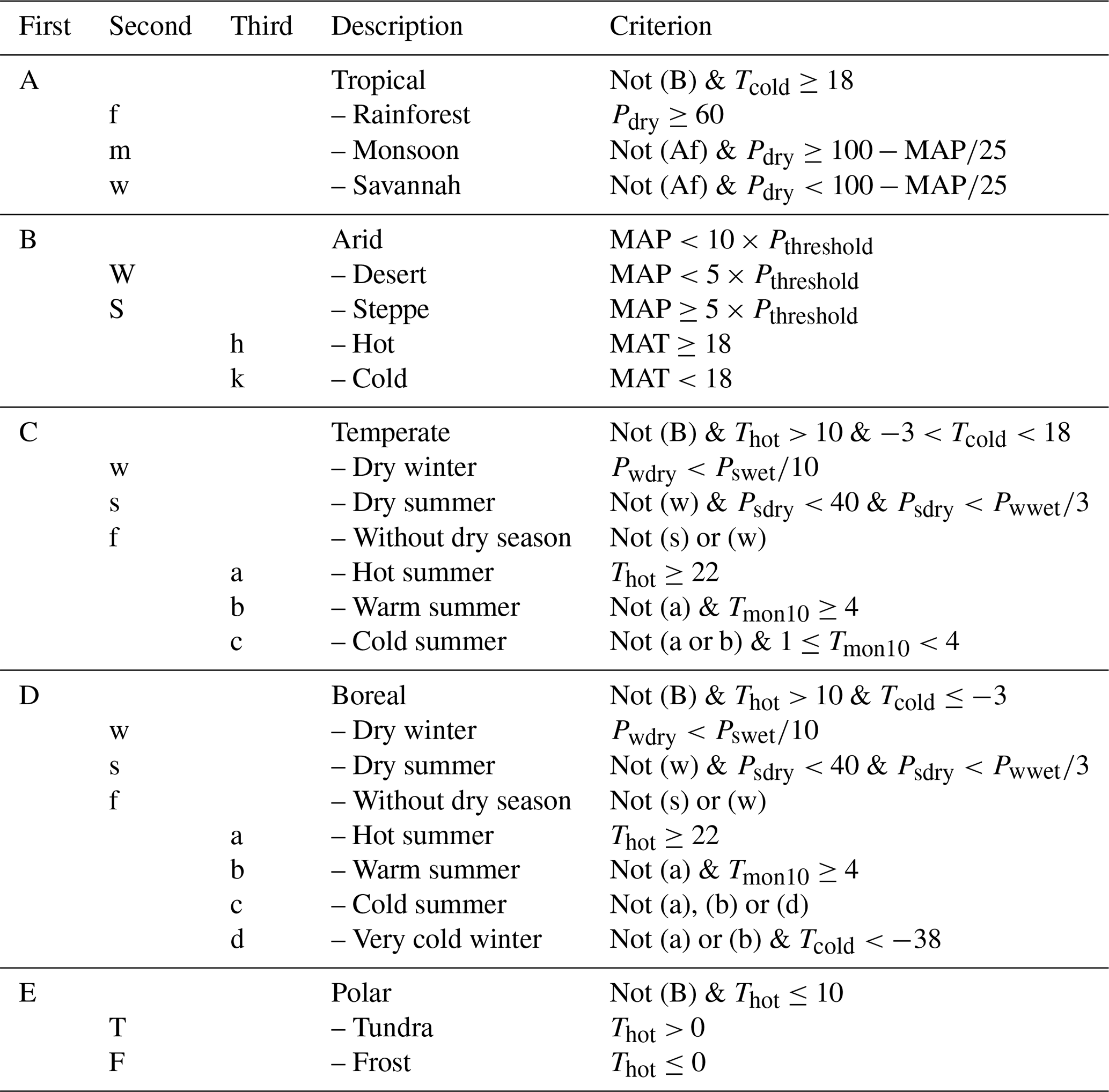
MAT: mean annual air temperature (∘C); Tcold: the air temperature of the coldest month (∘C); Thot: the air temperature of the warmest month (∘C); Tmon10: the number of months with air temperature > 10 ∘C; MAP: mean annual precipitation (mm yr−1); Pdry: precipitation in the driest month (mm per month); Psdry: precipitation in the driest month in summer (mm per month); Pwdry: precipitation in the driest month in winter (mm per month); Pswet: precipitation in the wettest month in summer (mm per month); Pwwet: precipitation in the wettest month in winter (mm per month); if > 70 % of precipitation falls in winter, if > 70 % of precipitation falls in summer, otherwise .
This research followed the Köppen–Geiger climate classification as described in Kottek et al. (2006) and Rubel and Kottek (2010). This latest version of the KGC scheme was first presented by Geiger (1961) (Table 2). Several existing Köppen–Geiger climate map products, including Peel et al. (2007), Kriticos et al. (2012), and Beck et al. (2018), applied the KGC scheme modified following Russell (1931). Russell (1931) adjusted the definition of the boundary of temperate (C) and boreal (D) climate zones using the coldest monthly temperature > 0 ∘C instead of > −3 ∘C. This threshold was proposed because the 0 ∘C line fits the distribution of the topographical features and vegetation in the western United States, where at that time meteorological stations were sparsely distributed (Jones, 1932). However, the application of 0 ∘C boundary to the global climates has not been validated. Therefore, this research did not utilize the Russell (1931) modification and followed the latest version KGC proposed by Geiger (1961).
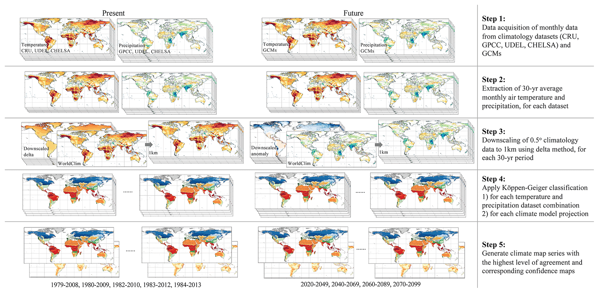
Figure 2Step-by-step process to generate Köppen–Geiger climate map series.
3.2 Statistical downscaling
Due to limited number of available observational datasets with high resolution and long-term continuous temporal coverage, the research implemented the delta method by applying a delta change or change factor (Hay et al., 2000; Wilby and Wigley, 1997) onto the WorldClim historical observations (Fick and Hijmans, 2017) to achieve 30-year average climatology data with a 1 km resolution based on the CRU, UDEL, and GPCC datasets. The delta method is a statistical downscaling method that assumes that the relationship between climatic variables remains relatively constant at local scale (Wilby and Wigley, 1997). We applied the delta method to downscale the long-term (30-year) mean climates using coarse-resolution monthly climatology datasets. The delta changes or change factors are calculated as the differences between the 30-year long-term means of temperature or precipitation of baseline (1970–2000) and present-day climates. The delta method comprises the following four steps: (1) calculate 30-year averages for the baseline (1970–2000) and present day of monthly temperature and precipitation, (2) calculate anomaly for precipitation and delta for temperature, (3) apply thin-plate spline (TPS) interpolation to create 1 km surface of precipitation anomaly and temperature delta, and (4) multiply anomaly or add delta to historical climates based on WorldClim dataset (Fig. 1).
First, using monthly time series from the CRU, UDEL, and GPCC datasets, we calculated 30-year means as a baseline (1970–2000) for each climatology dataset and each variable. We used 1970–2000 as the baseline period, for consistency with WorldClim Historical Climate Data V2. Next, we calculated 30-year means for each month and each 30-year present-day period in 1979–2013. We then calculated anomalies as proportional differences between present day and baseline in total precipitation and delta as the difference in temperature. To derive 30 arcsec (1 km) anomaly or delta surfaces, we applied thin-plate spline (TPS) interpolation (Franke, 1982; Schempp et al., 1977; Craven and Wahba, 1978) to precipitation anomaly and temperature delta. TPS has been widely used in climate science (Hijmans et al., 2005; Navarro-Racines et al., 2020) as it produced a smooth and continuous surface, which is infinitely differentiable. Last, we multiplied the change factor or added the delta to the WorldClim (1970–2000) data to get downscaled present-day monthly climate data.
Our future Köppen–Geiger map series are based on an ensemble of maps derived from the CCAFS bias-corrected and downscaled climate projections, which include 35 CMIP5 GCMs and 4 RCPs (Navarro-Racines et al., 2020). Large misclassifications exist within the GCMs as detected in previous assessments of large areas ranging between 20 %–50 % of the total land area (Cui et al., 2021a). Deficiencies in model physics are also more likely to contribute to uncertainties in the maps than grid size or reference dataset limitations (Tapiador et al., 2019). Multi-model mean and delta-change methods can mitigate the bias effects from the threshold-based classification scheme and have been utilized to simulate better results of climate classification (Hanf et al., 2012). Therefore, we chose the CCAFS bias-corrected and downscaled CMIP5 projections (Navarro-Racines et al., 2020) to reduce the amplified errors due to uncertainty of climate projections. Navarro-Racines et al. (2020) interpolated anomalies of original GCM outputs using thin plate spline spatial interpolation to achieve a baseline climate with a 1 km surface. Then they applied the delta method to the interpolated baseline climates to correct the model biases (Hay et al., 2000; Ho et al., 2012).
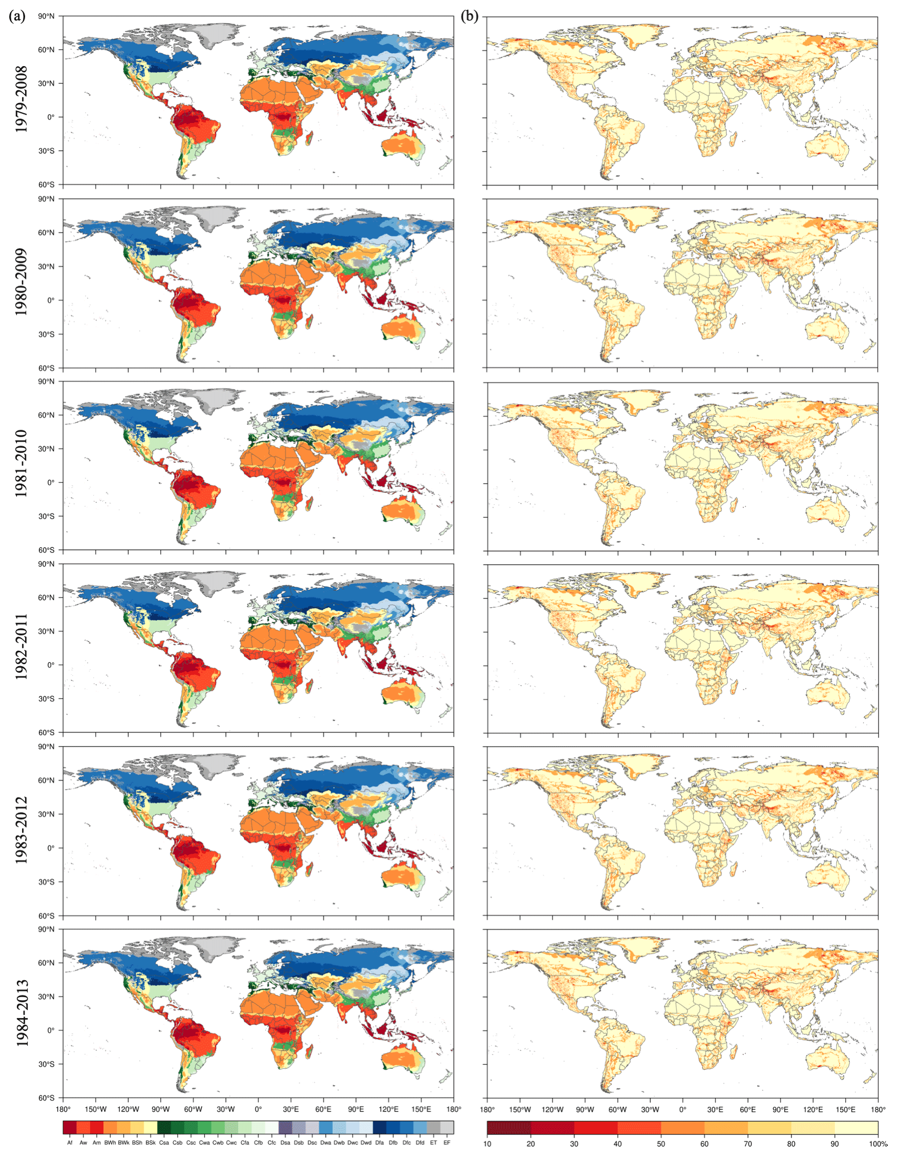
Figure 3Global maps of the Köppen–Geiger climate classification for the historical periods (1979–2008, 1980–2009, 1981–2010, 1982–1011, 1983–2012, 1984–2013) and associated classification confidence levels. (a) Historical maps of the Köppen–Geiger climate classification and (b) confidence levels associated with the Köppen–Geiger climate classification.
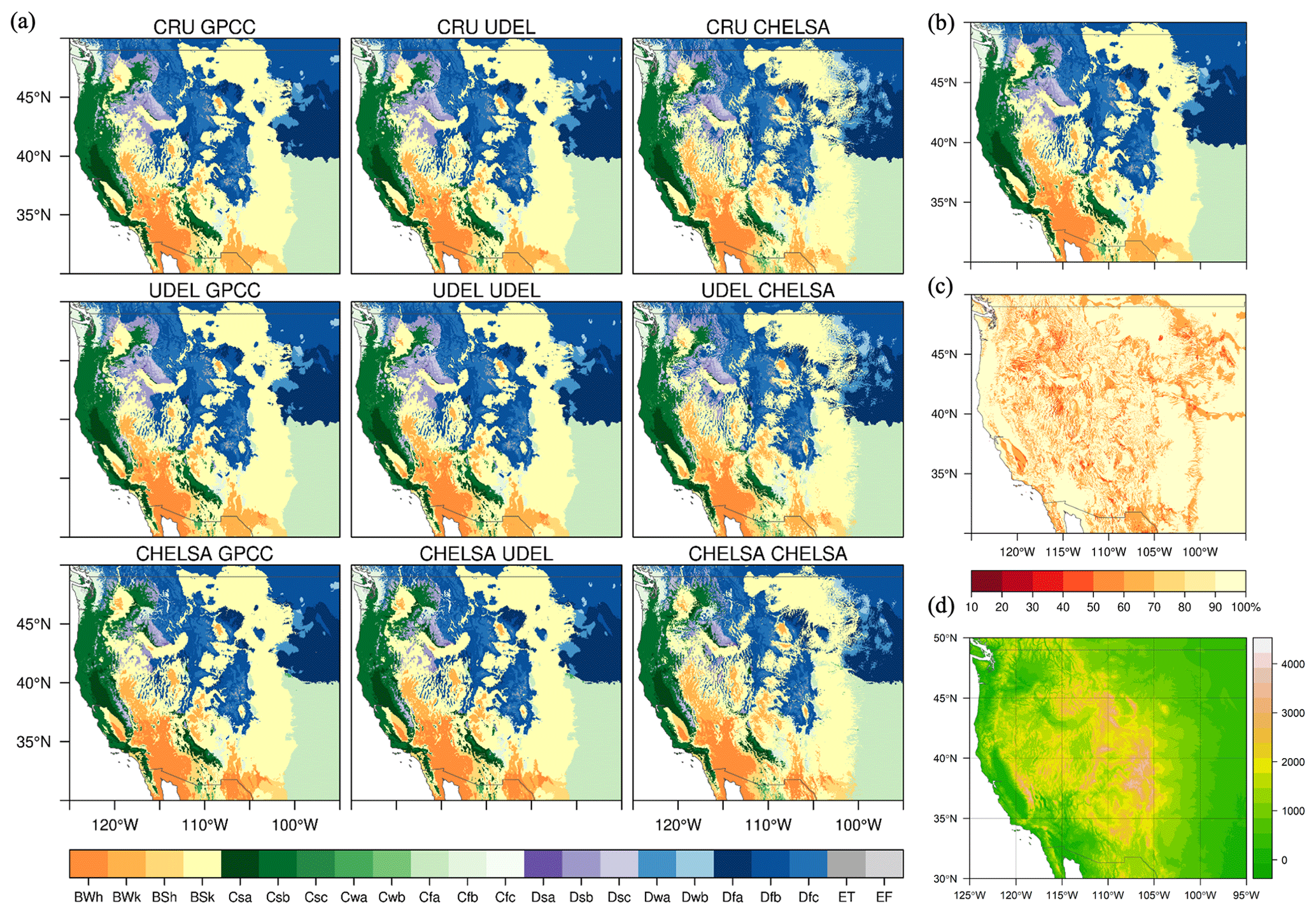
Figure 4Present Köppen–Geiger classification and confidence map for 1979–2008 with resolution of 1 km for the central Rocky Mountains in North America. (a) Climate maps based on the nine combinations of the three precipitation datasets and three surface air temperature datasets, (b) the final climate map derived from the most common climate class among the nine climate maps, (c) confidence level distribution of the final climate map, and (d) elevation map for the central Rocky Mountains in North America.
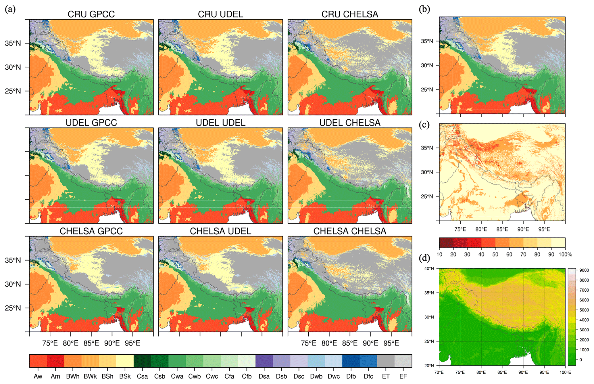
Figure 5Present Köppen–Geiger classification and confidence map for 1979–2008 with resolution of 1 km for the Tibetan Plateau. (a) Climate maps based on the nine combinations of the three precipitation datasets and three surface air temperature datasets, (b) the final climate map derived from the most common climate class among the nine climate maps, (c) confidence level distribution of the final climate map, and (d) elevation map for the Tibetan Plateau.
3.3 Data integration
The historical Köppen–Geiger climate classification map series was generated using the highest confidence class from an ensemble of maps using all combinations of surface air temperature and precipitation products (Fig. 2), as described in Beck et al. (2018). The highest confidence was given to the most common climate class for each grid cell. The final historical climate map series were derived using the climate class with the highest level of confidence in an ensemble of 3 × 3 = 9 classification maps based on combinations of the three precipitation datasets (CRU, UDEL, and CHELSA) and three surface air temperature datasets (GPCC, UDEL, and CHELSA). To further test the sensitivity of the method using the climate with the highest level of agreement, we incorporated another data integration method using the mean of multiple datasets. We quantified the degree of confidence placed in the Köppen–Geiger climate map series using the degree of confidence at the grid cell level calculated by dividing the occurrence frequency of the climate class with the highest level of agreement by the ensemble size. The calculated confidence level can be viewed as the agreement degree in classification derived from different climatology datasets.
The future Köppen–Geiger climate classification map series under four RCPs were derived based on the most common climate class from an ensemble of future climate maps. We generated a future Köppen–Geiger climate classification map for each climate model projection, using the CCAFS bias-corrected and downscaled CMIP5 GCM dataset. For example, the future Köppen–Geiger climate classification map series under RCP8.5 was derived from an ensemble of 30 maps based on 30 CMIP5 models. The level of confidence was estimated using the ratio between the frequency of the climate class with the highest level of agreement in the future map results and the ensemble size.
3.4 Validation
We validated the historical climate maps using the station observations from Global Historical Climatology Network-Daily (GHCN-D) (Menne et al., 2012) and Global Summary of the Day (GSOD) database (National Climatic Data Center et al., 2015) as reference data. The GHCN-D dataset provides daily climate data over global land areas and contains records from over 80 000 weather stations worldwide, about one-third of which have both temperature and precipitation data available (Menne et al., 2012). The GSOD dataset includes global daily summary data over 9000 stations, of which the historical data from 1973 are the most complete (National Climatic Data Center et al., 2015). For each station, time series of monthly temperature and precipitation were calculated from the daily observations with months with <15 daily values discarded. Then if ≥ 6 months are present, monthly climatologies were subsequently generated by averaging the monthly means for the given 30-year period. We removed duplicate stations in the two datasets and discarded stations with gap years or missing data in the given 30 years. For each station and each 30-year period, we applied the Köppen–Geiger climate classification, and then we evaluated overall classification performance for each climate map using total accuracy, which is defined as the percentage of correct classes and average precision, which is the averaged fraction of correct classification for all climate classes.
Using the same validation datasets and station selection process, we also evaluated the previous climate maps from Beck et al. (2018), Kriticos et al. (2012), Peel et al. (2007), and Kottek et al. (2006). We applied the same Köppen–Geiger climate classification criteria described in the previous studies to assess the overall accuracy of the map products. To further validate the climate classification results, we performed sensitivity analysis on the data integration method, the climate classification timescale, and climatology dataset input, using the same validation datasets from GHCN-D and GSOD. In addition, we compared the climate classification results with forest cover and elevation maps and with the two high-resolution comparable climate map products, Beck et al. (2018) (1 km) and Kriticos et al. (2012) (0.167∘), at regional and continental scales. The forest cover map we used is the 2000 30 m Landsat-based forest cover map (Hansen et al., 2013). The elevation data are from the NASA SRTM Digital Elevation 30 m data (Farr et al., 2007).
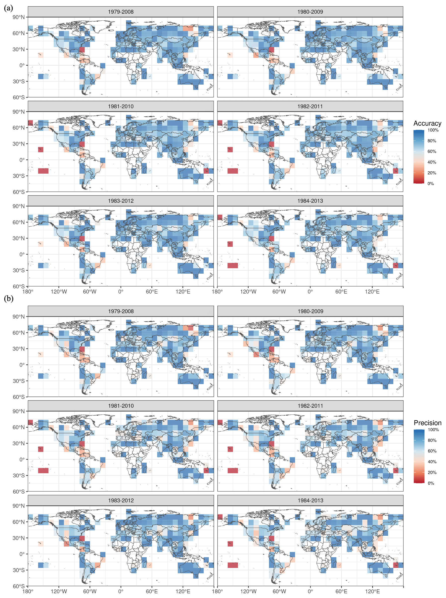
Figure 6Validation of the historical Köppen–Geiger climate map series (1979–2008, 1980–2009, 1981–2010, 1982–2011, 1983–2012, 1984–2013). (a) Small-scale accuracy of historical Köppen–Geiger climate maps. (b) Small-scale precision of historical Köppen–Geiger climate maps. Climate classification has been applied for each station. The small-scale accuracy and precision are calculated based on the classification results of all the stations within the given region, with a minimum of three stations in the 5∘ search radius.
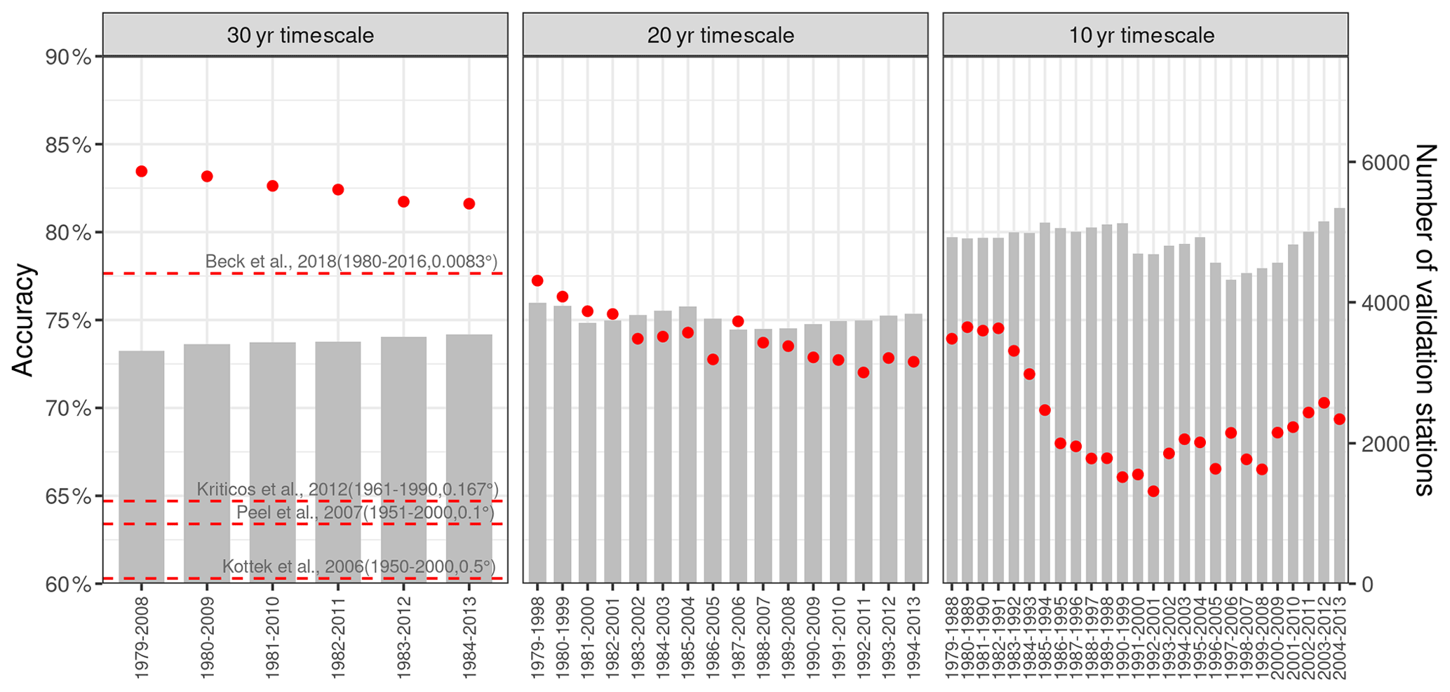
Figure 7Validation of downscaled data of bioclimatic variables and the generated Köppen–Geiger climate map.
4.1 Historical Köppen–Geiger climate maps
Global map series of the Köppen–Geiger climate classification for historical periods and associated corresponding confidence levels are shown in Fig. 3. Based on the distribution of confidence level, over 90 % of the land area exhibits a high level of confidence as classification results based on different climate data show excellent agreement. Relatively lower confidence level and large discrepancy in classification results are found in particular in mountainous regions such as the Andes Mountains, Rocky Mountains, Tibetan Plateau, and major climate transitional zones located in the midlatitude and high latitudes of Northern Hemisphere, central Africa, and central Asia.
Regional distributions of climatic conditions are largely created by local variation in topography in rugged terrain (Dobrowski et al., 2013; Franklin et al., 2013). The climate classification and confidence level maps of mountainous areas of the central Rocky Mountains and Tibetan Plateau are shown in Figs. 4 and 5, respectively. For each combination of precipitation and surface air temperature datasets, we generated a Köppen–Geiger climate classification map (see Figs. 4a and 5a for 1979–2008 maps for the central Rocky Mountains and Tibetan Plateau). The final Köppen–Geiger classification map is derived based on the most common climate type among all the climate maps (Figs. 4b and 5b). We then calculated corresponding confidence levels to quantify the uncertainty in the classification maps (Figs. 4c and 5c). The uncertainty in climate classification in mountainous areas is attributed to the uncertainty existing in climate data, especially precipitation data. In rugged terrain, CHELSA precipitation data show more detailed precipitation patterns, causing disagreement in classification results of the third-level climate classes which depict precipitation seasonality.
4.2 Validation
We validated the historical climate maps using the station observations from Global Historical Climatology Network-Daily (GHCN-D) (Menne et al., 2012) and Global Summary of the Day (GSOD) database (National Climatic Data Center et al., 2015). Figure 6 shows the small-scale distributions of total accuracy and average precision for historical Köppen–Geiger climate map series with 10∘ grid cells. Due to uneven distributions of weather stations, remote areas in the Pacific islands, central Africa, and Amazon forest suffer from a lack of station observations or underrepresented validation results.
Table 3Continental and global overall accuracy, average precision, and confidence level of the historical Köppen–Geiger climate map series (1979–2008, 1980–2009, 1981–2010, 1982–2011, 1983–2012, 1984–2013). The overall accuracy is calculated as the percentage of correct climate classes using ground observations, and average precision is the averaged fraction of correct classification for all climate classes. Confidence level values show the 95 % confidence interval of the confidence level for each continent and the whole globe. All the values are presented as percentages.
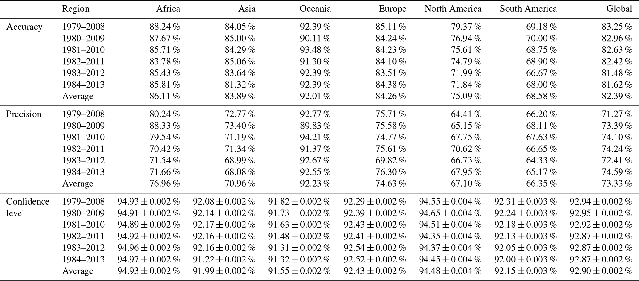
We summarized the overall accuracy, average precision, and confidence levels for each continent and the whole globe (Table 3). The global overall classification accuracy of the historical Köppen–Geiger climate maps is estimated to be 82.39 %, with the lowest in South America (68.58 %) and highest in Oceania (92.01 %). The global average precision, which is calculated as averaged fraction of correct classification for all climate classes, is 73.33 %. Similar to overall accuracy, South America has the lowest precision level, equal to 66.35 %, and Oceania the highest, 92.23 %. Having a good correspondence with accuracy and precision values, the continental average confidence levels range from 91.55 % to 94.93 %, and the global level is 92.90 % (Table S2). Overall, the spatial patterns of total accuracy and average precision show good correspondence with classification confidence levels (Fig. 3), indicating a potential of confidence level to represent classification uncertainty.
Table 4Accuracy of the 1 km Köppen–Geiger climate map series derived from different combinations of temperature and precipitation dataset input and by different means of integration of multiple datasets. The values represent overall accuracy based on the technical validation using ground observation as reference.

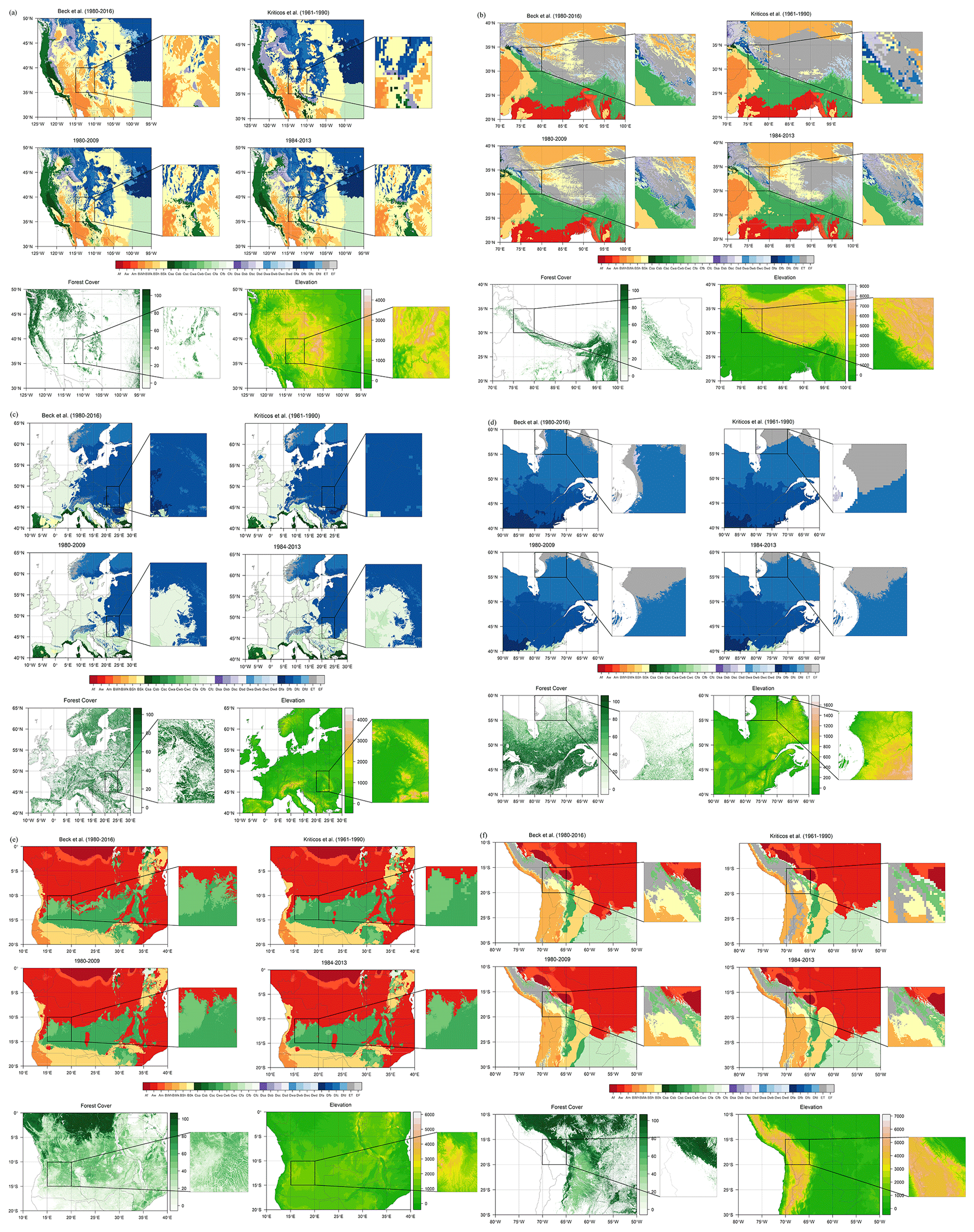
Figure 8Köppen–Geiger climate classification maps from previous studies, Beck et al. (2018, 1 km, 1980–2016) and Kriticos et al. (2012, 0.167∘, 1961–1990), and our study (1 km, 1979–2009 to 1984–2013) and associated forest cover and elevation maps, for regions with large spatial gradients in climates or sharp elevation gradients. (a) Central Rocky Mountains, (b) Tibetan Plateau, (c) Europe, (d) high latitudes in North America, (e) central and eastern Africa, and (f) central Andes. The forest cover map is the 30 m Landsat-based forest cover map for the year 2000 (Hansen et al., 2013). The elevation data are the NASA SRTM Digital Elevation 30 m data (Farr et al., 2007). The representative period of each map is listed in parentheses.
Using the same validation datasets from GHCN-D and GSOD, we tested sensitivity of the climate map series using different combinations of temperature and precipitation datasets and different methods of data integration (Table 4). Results indicated an average total accuracy of the 1 km Köppen–Geiger classification maps generated with all the CHELSA and downscaled CRU, GPCC, and UDEL datasets and with only downscaled CRU, GPCC, and UDEL datasets as 82.39 % and 81.17 %, respectively. Using the mean of multiple datasets, which can potentially reduce the data bias, led to better classification results. We estimated the total accuracy of the previous high-resolution Köppen–Geiger climate map products using the same validation datasets. We applied the same classification system described in the previous studies and the same time period of the previous climate map product to process the station observation data and estimate their overall accuracy. Compared with the previous high-resolution Köppen–Geiger climate map products, Beck et al. (2018) and Kriticos et al. (2012), the newly generated Köppen–Geiger climate map series showed greater accuracy in total.
We conducted sensitivity analysis of the Köppen classification scheme and tested multiple timescales, 10 years, 20 years, and 30 years. The selection criteria of station observations were adjusted accordingly based on the timescale utilized. Accuracy results exhibited decreasing accuracy for shorter timescales (Fig. 7). Further, we estimated the total accuracy for the Köppen–Geiger climate classification maps from previous studies, Beck et al. (2018) Kriticos et al. (2012), Peel et al. (2007), and Kottek et al. (2006), using the same validation dataset and consistent Köppen–Geiger climate classification scheme the corresponding study applied. The validation results demonstrate that the new Köppen–Geiger maps have comparatively higher overall accuracy than all the previous studies.
4.3 Regional- and continental-scale comparison
At the regional and continental scale, we compared our Köppen–Geiger climate classification maps with previous map products for regions with large spatial gradients in climates, including central and eastern Africa, Europe, and North America, and regions with sharp elevation gradients, including the Tibetan Plateau, central Rocky Mountains, and central Andes (Fig. 8). We compared the new 1 km Köppen–Geiger climate classification maps from our study for time periods of 1980–2009 and 1984–2013 with the high-resolution Köppen–Geiger maps from two previous studies, Beck et al. (2018), which has a resolution of 1 km and temporal coverage of 1980–2016, and Kriticos et al. (2012), which has a resolution of 0.0167∘ and covers 1961–1990. The Köppen classifications demonstrate good correlation with natural landscape distributions (Belda et al., 2014; Köppen, 1936; Trewartha, 1954). To show the agreement between the improved Köppen–Geiger climate classification maps and regional landscape distributions, we also showed maps of forest cover and elevation distribution for these regions. Figure 8 illustrates the enhanced regional details of the maps.
Compared with the Köppen–Geiger climate maps from previous studies with only one time period, the series of the Köppen–Geiger climate maps from our study demonstrate the ability to capture recent changes in spatial distributions of climate zones. For example, our maps can detect the significant changes in the climate zones specifically driven by the accelerated global warming since the 1980s, for example, the poleward movements of boreal (D) and polar (E) climates in high latitudes in North America shown in the comparison between the 1980–2009 and 1984–2013 Köppen–Geiger climate maps (Fig. 8d). Another example is the expansion of savanna (Aw) climate into the temperate (Cw) climate zone, witnessed in central Africa (Fig. 8e).
Another improvement of the new series of the Köppen–Geiger climate maps is the application of a threshold of −3 ∘C as the boundary of temperate (C) and boreal (D) climate zones, which show better agreement with global boreal forest distributions at the regional scale compared with the Russell (1931) modification of 0 ∘C, which Beck et al. (2018) and Kriticos et al. (2012) utilized. Based on the comparison results of the Köppen climate zones and the biome classifications from the World Wildlife Federation (Rohli et al., 2015b), the boreal (D) climate zone largely corresponds to the distribution of boreal forest (Cui et al., 2021a). For example, evidenced in Fig. 8c, the new Köppen–Geiger climate classification maps from our study show better agreement with the boreal forest in the Carpathian Mountains across central and eastern Europe than Beck et al. (2018) and Kriticos et al. (2012). Figure 8d also shows good agreement of the northern boundary of the boreal (D) climate zone in the northern part of Quebec in Canada with the boundary of Canada's boreal forest.
Moreover, the new Köppen–Geiger maps can show an accurate depiction of important topographic features over the regions with complex topography. For example, the topo-climate of the Himalayas' southern front determined by the mountain ranges is represented with more detail in the new Köppen–Geiger maps compared with Beck et al. (2018) and Kriticos et al. (2012) (Fig. 8b). The abrupt changes in climate along the edges of the Andes mountains are also well described in the new maps (Fig. 8f).
In addition, the distribution of tropical (A), temperate (C), and boreal (D) climate zones in the new Köppen–Geiger maps correspond closely with tree lines in the forest cover maps. The temperate (C) and boreal (D) climate distributions based on the Köppen–Geiger maps show a better agreement with the forest distributions of the middle and southern Rocky Mountains than Beck et al. (2018) and Kriticos et al. (2012) (Fig. 8a). For another example, the boundaries of the tropical rainforest in central Africa and South America are clearly delineated in the new Köppen–Geiger maps (Fig. 8e and f).
4.4 Bioclimatic variables
Beyond the Köppen–Geiger climate classification maps, we calculated a set of bioclimatic variables from the monthly climate data (see full list in Table 5). The bioclimatic variables at 1 km spatial resolution can capture regional environmental variations in particular in mountainous areas and areas with strong climate variations. These bioclimatic variables can be used in studies of environmental, agricultural, and biological sciences, for example, development of species distribution modeling and assessment of biological impacts induced by climate change. The variables provide descriptions of annual averages and seasonality of climates. The warmest half year or the coldest half year is defined as the period of the warmest 6 months or the coldest 6 months.
Table 5List of bioclimatic variables derived from downscaled monthly climate data.

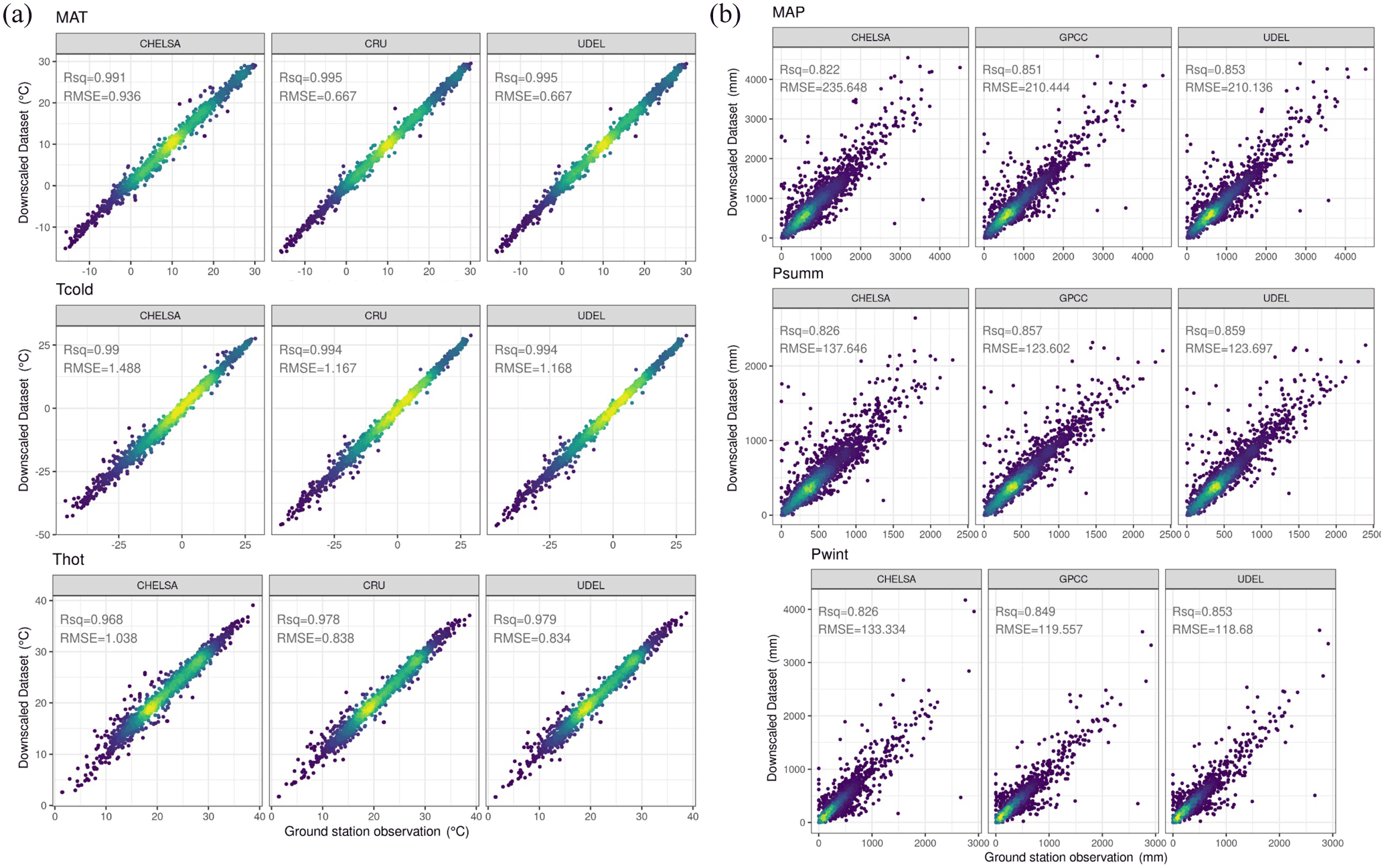
Figure 9Scatter plots of the station observations and estimates of bioclimatic variables from downscaled climatology data. The bioclimatic variables include the 30-year means of annual temperature (MAT), the air temperature of the coldest month (Tcold), the air temperature of the warmest month (Thot), total annual precipitation (MAP), precipitation of the summer half year (Psumm), and precipitation of the winter half year (Pwint). (a) Scatter plots of the station observations and downscaled temperature data from CHELSA, CRU, and UDEL datasets and (b) downscaled precipitation data from CHELSA, GPCC, and UDEL datasets.
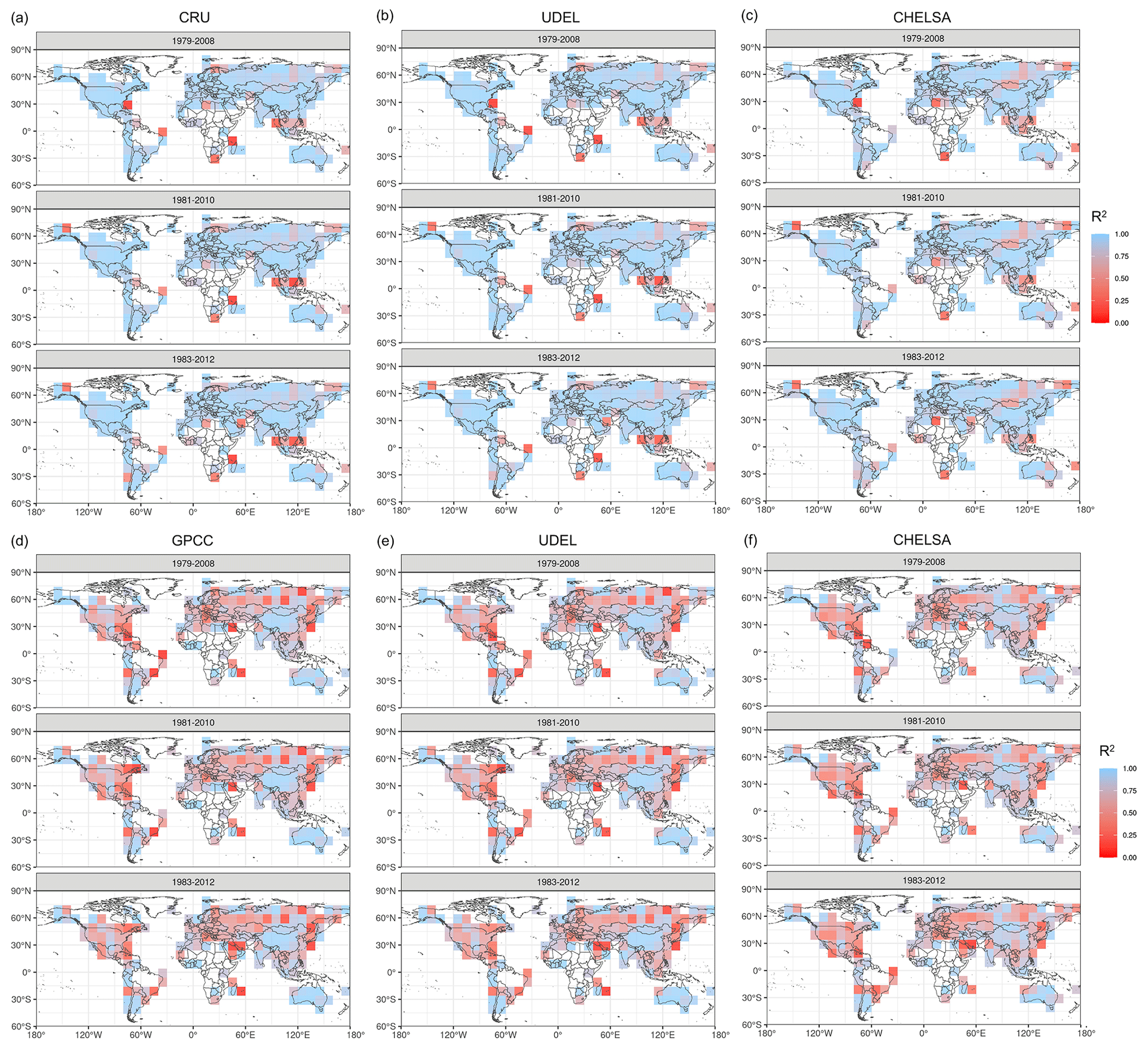
Figure 10Small-scale comparison of annual temperature (MAT) and mean annual precipitation (MAP) variables derived from different datasets with station data. Small-scale correlation between the 30-year average mean annual temperature (MAT) and mean annual precipitation (MAP) data and ground observations for three historical periods (1979–2008, 1981–2010, 1983–2012). The station data are from GHCN-D and the GSOD database. The figure shows the R2 value for 10∘ grid cells. Panels (a), (b), and (c) are MAT results. Panels (d), (e), and (f) are MAP results. (a) MAT is calculated from downscaled monthly temperature data from the CRU dataset, (b) from the UDEL dataset, and (c) from the CHELSA dataset. (d) MAP is calculated from downscaled monthly precipitation data from the GPCC dataset, (e) from the UDEL dataset, and (f) from the CHELSA dataset.
We validated the bioclimatic variables from different datasets with station data from GHCN-D (Menne et al., 2012) and the GSOD database (National Climatic Data Center et al., 2015) (Fig. 9). We calculated a linear regression model for the 12 bioclimatic variables for each 10∘ grid cell (Fig. 10). The 30-year average mean annual temperature (MAT) from the CHELSA dataset shows the overall highest fit with station data, with CRU, and UDEL datasets show a smaller but still strong correlation with station data. The 30-year average mean annual precipitation (MAP) estimates from the GPCC, UDEL, and CHELSA datasets have considerable uncertainties, indicated by relatively low correlation with station observations. In current precipitation datasets, there is a varied degree of discrepancy in annual estimates over multiple timescales (Sun et al., 2018).
4.5 Future Köppen–Geiger climate maps
Future Köppen–Geiger climate classification maps under RCP8.5 and associated confidence levels are shown in Fig. 11. Indicated by confidence levels, there exist larger uncertainties in the final future climate maps than historical maps, particularly at midlatitudes and high latitudes. The climate map for the future period of 2070–2099 shows the largest uncertainty compared with the other future periods.
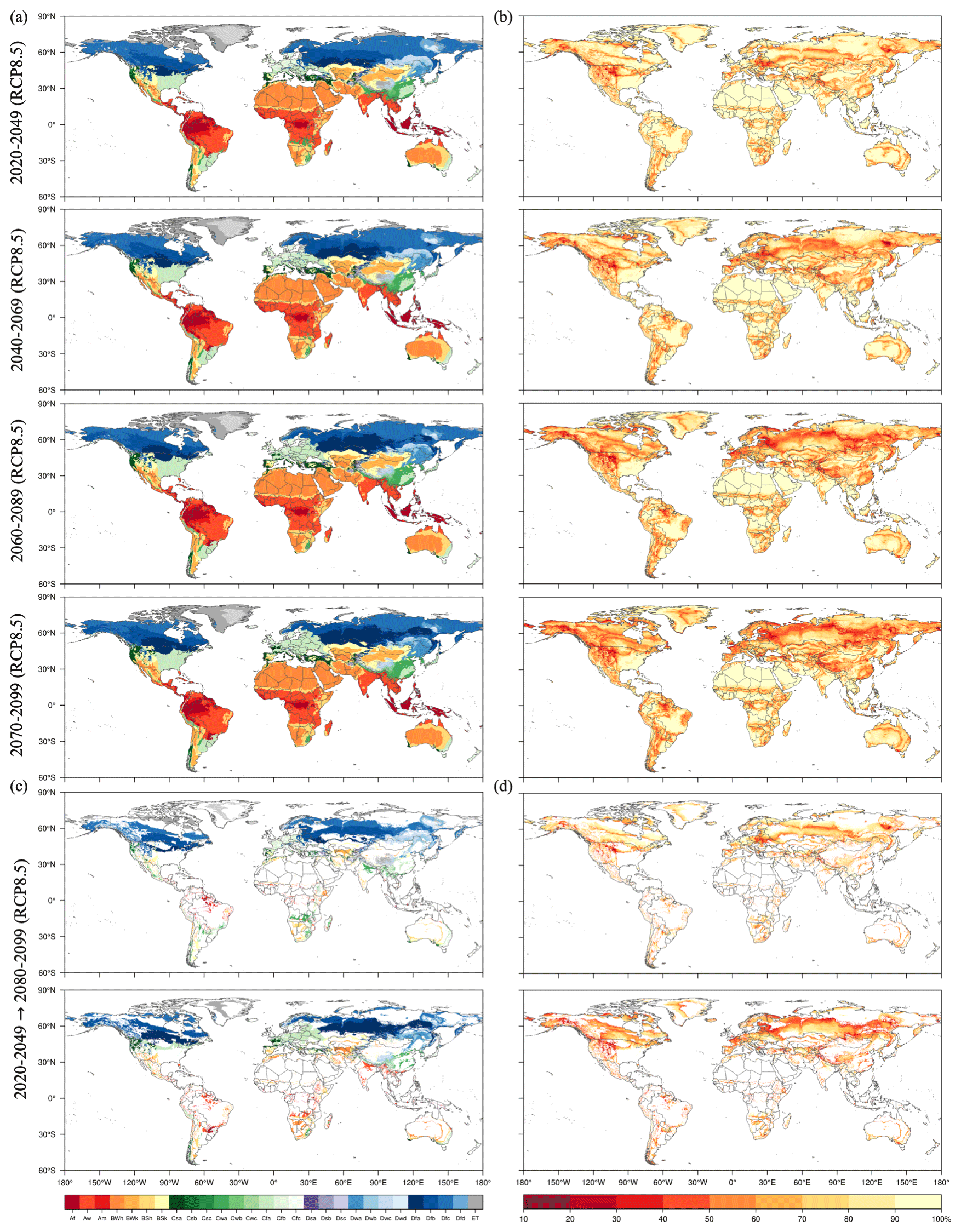
Figure 11Global maps of the Köppen–Geiger climate classification for the future periods (2020–2049, 2040–2069, 2060–2089, 2070–2099) under RCP8.5 and associated classification confidence levels. (a) Future maps of the Köppen–Geiger climate classification and (b) confidence levels associated with the Köppen–Geiger climate classification. (c) Future changes in Köppen–Geiger climates from 2020–2049 to 2080–2099 and (d) the associated confidence levels.
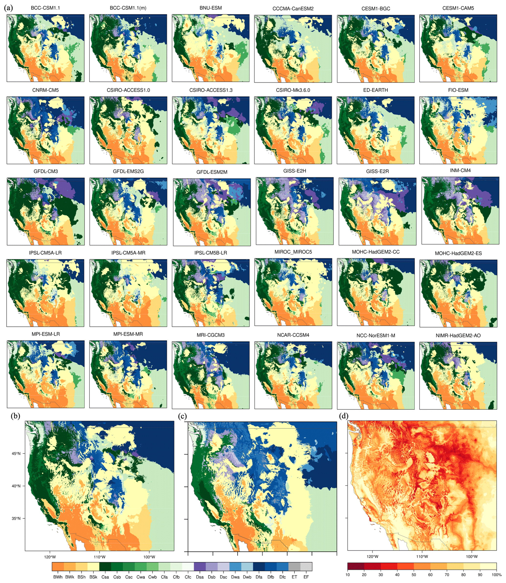
Figure 12Future Köppen–Geiger classification and confidence map for 2060–2089 under RCP8.5 with resolution of 1 km for the central Rocky Mountains in North America. (a) Climate maps based on 30 GCMs, (b) the final climate map derived from the most common climate class among all the 30 climate maps, (c) present climate map of 1979–2008, and (d) confidence level distribution of the final climate map.
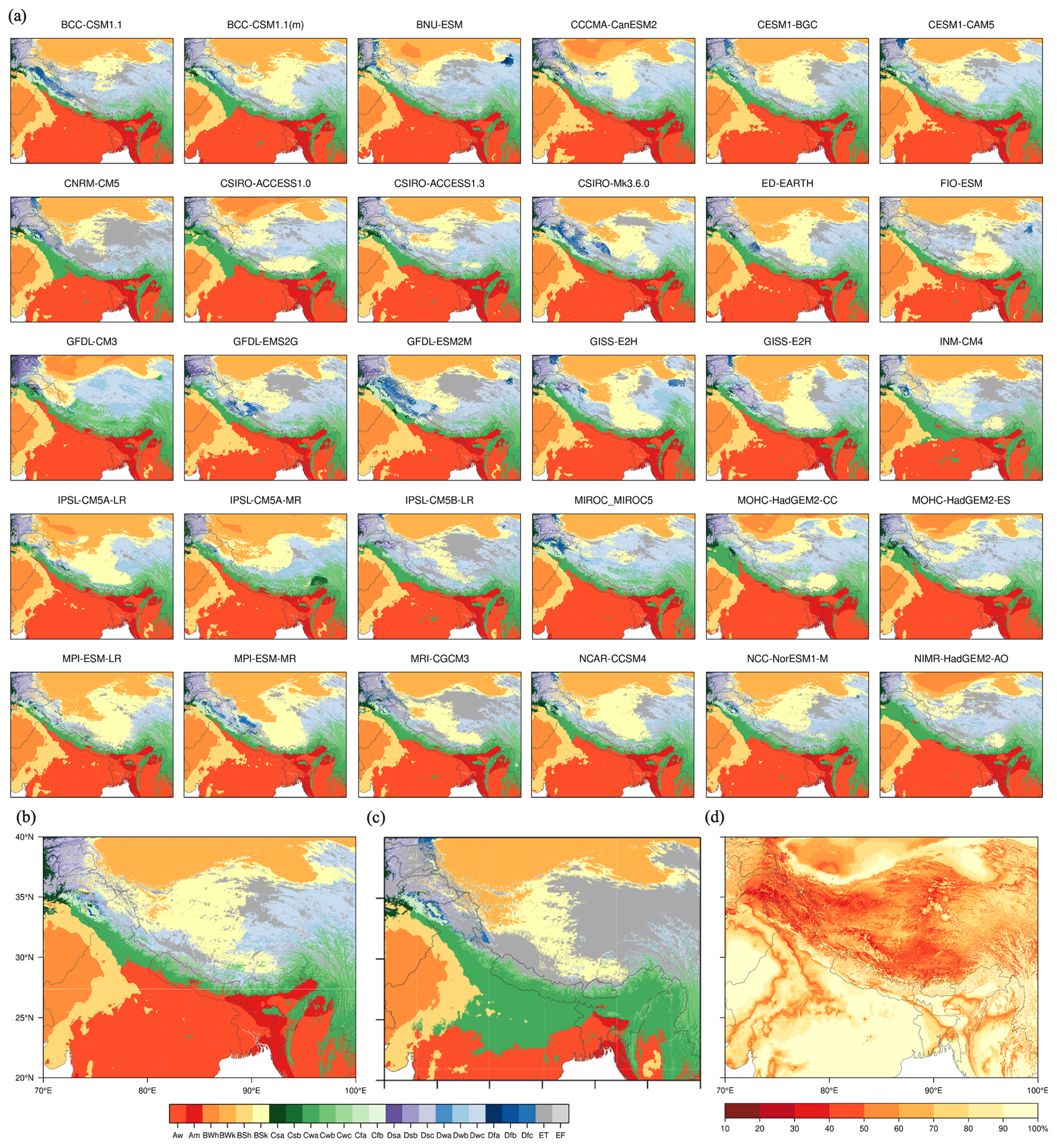
Figure 13Future Köppen–Geiger classification and confidence map for 2060–2089 under RCP8.5 with resolution of 1 km for the Tibetan Plateau. (a) Climate maps based on 30 GCMs, (b) the final climate map derived from the most common climate class among all 30 climate maps, (c) present climate map of 1979–2008, and (d) confidence level distribution of the final climate map.
Future climate classifications derived from the diverse GCM projections for four RCPs, which are inherently uncertain (Winsberg, 2012; Gleckler et al., 2008), provide a proxy of global distributions of climatic conditions and can represent potential spatial changes in climate zones under global warming. The large uncertainty and strong disagreement in projected climate classification maps at high latitudes and in regions with rugged terrain can be indicated by relatively low confidence levels. Figures 12 and 13 show the future Köppen–Geiger climate classification maps based on GCM projections under RCP8.5 and associated confidence levels for the central Rocky Mountains and Tibetan Plateau. We generated a future Köppen–Geiger climate classification map for each bias-corrected and downscaled CMIP5 GCM projection (see Figs. 12a and 13a for 2070–2099 maps for the central Rocky Mountains and Tibetan Plateau). Noticeable regional changes in climate zones have been projected by comparing the 2070–2099 and 1979–2008 climate classification maps (see Fig. 12b and c for the central Rocky Mountains and Fig. 13b and c for the Tibetan Plateau).
4.6 Application example: detection of area changes in climate zones
Changes in climatic conditions under global warming have significant impacts on biodiversity and ecological systems. Area changes of climate zones can indicate spatial shrinkage or expansion of analogous climatic conditions, potentially implying threats for species range contraction or opportunities for range expansion (Cui et al., 2021a). To examine the area changes of climate zones, we calculated the total area covered by each climate type for each historical and future period under the high-emission RCP8.5 scenario (Fig. 14). Our results of changes in area occupied by different climate zones demonstrate good agreement with results from previous studies (Chan and Wu, 2015). Results show that accelerated anthropogenic global warming since the 1980s has caused large-scale changes in climate zones, and shifts into warmer and drier climates are projected in this century. The tropical and arid climates are expanding into large areas in midlatitudes, whereas the high-latitude climates will experience significant area shrinkage.
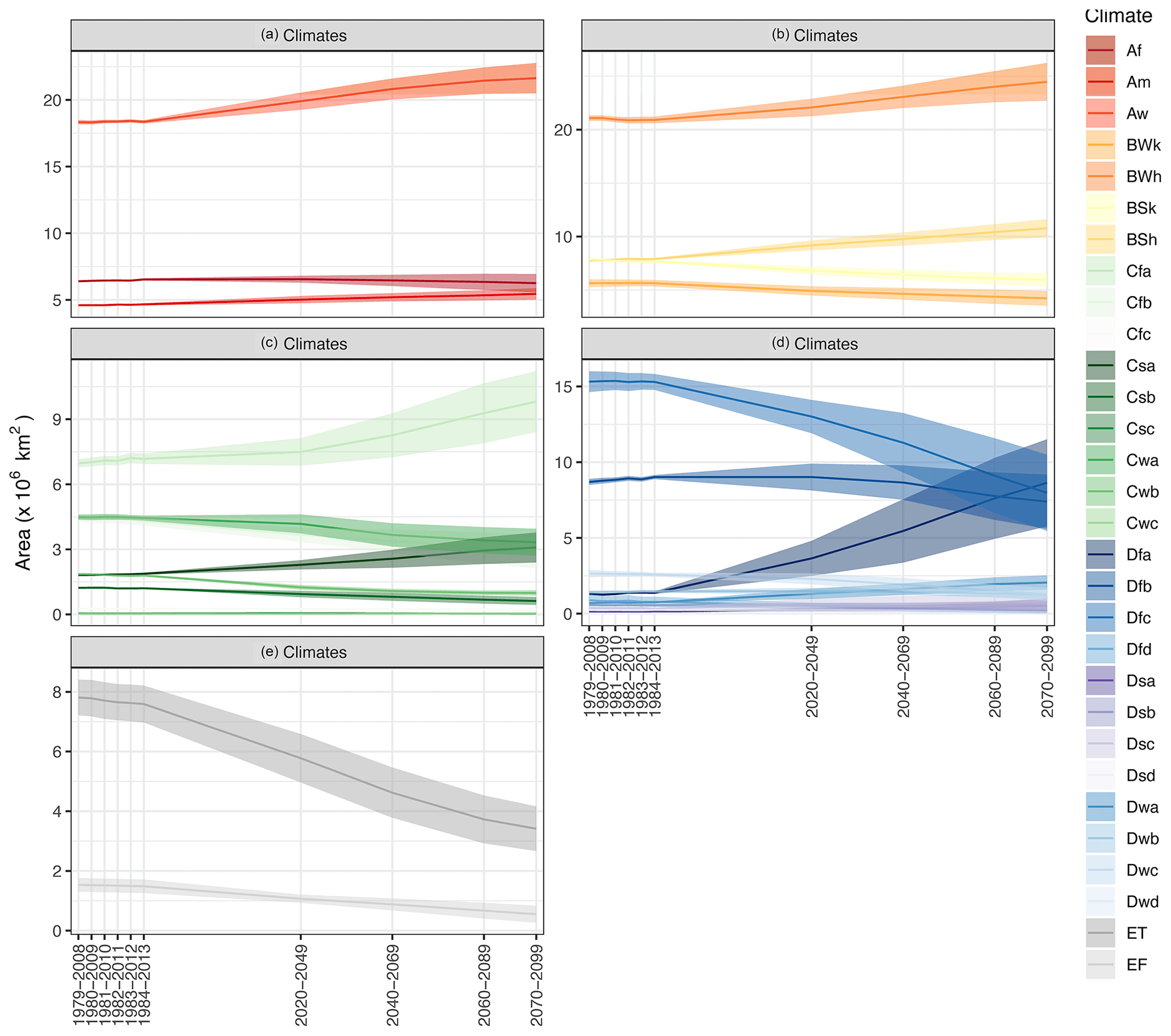
Figure 14Area changes in climate zones since the 1980s on a global scale under RCP8.5. The error bars for historical periods (1979–2014) indicate standard error in the Köppen–Geiger classification results based on the nine combinations of observational air temperature and precipitation datasets and for future periods (2020–2099); the error bars indicate standard error in the Köppen–Geiger classification results based on the 30 GCMs.
This high-resolution global dataset of the Köppen–Geiger climate classification and bioclimatic variable dataset is freely available via http://glass.umd.edu/KGClim (Cui et al., 2021d) and can also be downloaded at https://doi.org/10.5281/zenodo.5347837 (Cui et al., 2021c) for historical climate and https://doi.org/10.5281/zenodo.4542076 (Cui et al., 2021b) for future climate.
Changes in broadscale climatic conditions, driven by anthropogenic global warming, lead to the redistribution of species diversity and the reorganization of ecosystems. Distributions of the Earth's climatic conditions have been widely characterized based on the Köppen climate classification system. The Köppen climate classification maps require fine resolutions of at least 1 km to detect relevant microrefugia and promote effective conservation. Studies examining recent and future interannual or interdecadal changes in climate zones at the regional scale need more accurate depiction of fine-grained climatic conditions and continuous and longer temporal coverage.
We presented an improved long-term Köppen–Geiger climate classification map series for six historical 30-year periods in 1979–2013 and four future 30-year periods in 2020–2099 under RCP2.6, 4.5, 6.0, and 8.5. To improve the classification accuracy and achieve a resolution as fine as 1 km, we combined multiple datasets, including WorldClim V2, CHELSA V1.2, CRU TS v4.03, UDEL, and GPCC and bias-corrected downscaled CMIP5 model simulations from CCAFS. The historical climate maps are based on the most common climate type from an ensemble of climate maps derived from combinations of observational climatology datasets. The future climate maps are based on an ensemble of climate maps derived from 35 GCMs. We estimated the corresponding confidence levels to quantify the uncertainty in climate maps. We also calculated 12 bioclimatic variables at the same 1 km resolution using these climate datasets for the same historical and future periods to provide data of annual averages, seasonality, and stressful conditions of climates.
To validate the Köppen–Geiger climate classification maps, we used the station observations from GHCN-D and the GSOD database. Our validation results show that the new Köppen–Geiger maps have comparatively higher overall accuracy than all the previous studies. Although the new maps exhibit improved overall accuracy, relatively lower confidence level and larger discrepancy in classification results are found in particular in mountainous regions and major climate transitional zones located in midlatitude and high latitudes. The confidence levels can provide a useful quantification of classification uncertainty.
Compared with climate maps from previous studies with a single present-day period, the series of the Köppen–Geiger climate maps from our study demonstrate the ability to capture recent and future projected changes in spatial distributions of climate zones. On regional and continental scales, the new maps show accurate depictions of topographic features and correspond closely with vegetation distributions. Our Köppen–Geiger climate classification maps can offer a descriptive and ecologically relevant way to provide insights into changes in spatial distributions of climate zones.
One of the limitations is that the future Köppen–Geiger climate maps built on downscaled climate model projections exist unavoidable uncertainties. The classification agreement levels of GCMs are relatively low at high latitudes and in regions with rugged terrain. The main sources of model discrepancies and uncertainties are deficiencies in model physics and varied model resolution. The climate model outputs have coarse spatial resolution varying from 70–400 km and cannot represent future climate change at the same scale of 1 km as well as our baseline climatology. Through bias-correction and downscaling methods, we made assumptions that local relationships between climatic variables remain constant across different scales, leading to a compromise between spatial scale and climate model physics.
We also tested the sensitivity of classification results to different timescales, dataset input, and data integration methods. Results show that the 30-year timescale exhibited the highest accuracy results. Moreover, using the mean of multiple datasets from CHELSA, CRU, UDEL, and GPCC could lead to better classification results. Last, we provided a heuristic example which used climate classification map series to detect the long-term area changes of climate zones, showing how the new Köppen–Geiger climate classification map series can be applied in climate change studies. With improved accuracy, high spatial resolution, and long-term continuous time coverage, this global dataset of the Köppen–Geiger climate classification and bioclimatic variables can be used in conjunction with species distribution models to promote biodiversity conservation and to analyze and identify recent and future interannual or interdecadal changes in climate zones on a global or regional scale.
The supplement related to this article is available online at: https://doi.org/10.5194/essd-13-5087-2021-supplement.
DC designed the computational framework, performed data collection and processing, conducted validation and sensitivity analyzes, and wrote the manuscript. ZL contributed to the data processing. SL was involved in planning and supervised the work. DC, SL, DW, and ZL discussed the results and commented on the manuscript.
The contact author has declared that neither they nor their co-authors have any competing interests.
Publisher’s note: Copernicus Publications remains neutral with regard to jurisdictional claims in published maps and institutional affiliations.
We acknowledge the Department of Geographical Sciences (GEOG), University of Maryland for supporting the research work. We sincerely thank the editor and the reviewers for their comments and suggestions to help improve the paper.
This paper was edited by Giulio G. R. Iovine and reviewed by two anonymous referees.
Beck, C., Grieser, J., Rudolf, B., and Schneider, U.: A new monthly precipitation climatology for the global land areas for the period 1951 to 2000, Geophys. Res. Abstr., 7, 7154, available at: http://www.juergen-grieser.de/publications/publications_pdf/Beck_Grieser_Rudolf_EGU_05.pdf (last access: 3 November 2021), 2005.
Beck, H. E., Zimmermann, N. E., McVicar, T. R., Vergopolan, N., Berg, A., and Wood, E. F.: Present and future Köppen-Geiger climate classification maps at 1 km resolution, Scientific data, 5, 180214, https://doi.org/10.1038/sdata.2018.214, 2018.
Belda, M., Holtanová, E., Halenka, T., and Kalvová, J.: Climate classification revisited: From Köppen to Trewartha, Clim. Res., 59, 1–13, https://doi.org/10.3354/cr01204, 2014.
Belda, M., Holtanová, E., Kalvová, J., and Halenka, T.: Global warming-induced changes in climate zones based on CMIP5 projections, Clim. Res., 71, 17–31, https://doi.org/10.3354/cr01418, 2016.
Bockheim, J. G., Gennadiyev, A. N., Hammer, R. D., and Tandarich, J. P.: Historical development of key concepts in pedology, Geoderma, 124, 23–36, https://doi.org/10.1016/j.geoderma.2004.03.004, 2005.
Brugger, K. and Rubel, F.: Characterizing the species composition of European Culicoides vectors by means of the Köppen-Geiger climate classification, Parasite. Vector., 6, 333, https://doi.org/10.1186/1756-3305-6-333, 2013.
Chan, D. and Wu, Q.: Significant anthropogenic-induced changes of climate classes since 1950, Sci. Rep., 5, 13487, https://doi.org/10.1038/srep13487, 2015.
Chen, D. and Chen, H. W.: Using the Köppen classification to quantify climate variation and change: An example for 1901–2010, Environmental Development, 6, 69–79, https://doi.org/10.1016/j.envdev.2013.03.007, 2013.
Chen, I.-C., Hill, J. K., Ohlemüller, R., Roy, D. B., and Thomas, C. D.: Rapid range shifts of species associated with high levels of climate warming, Science, 333, 1024–1026, https://doi.org/10.1126/science.1206432, 2011.
Chen, M., Xie, P., Janowiak, J. E., and Arkin, P. A.: Global land precipitation: A 50-year monthly analysis based on gauge observations, J. Hydrometeorol., 3, 249–266, 2002.
Craven, P. and Wahba, G.: Smoothing noisy data with spline functions, Numer. Math., 31, 377–403, https://doi.org/10.1007/BF01404567, 1978.
Cui, D., Liang, S., and Wang, D.: Observed and projected changes in global climate zones based on Köppen climate classification, WIREs Clim. Change, 12, e701, https://doi.org/10.1002/wcc.701, 2021a.
Cui, D., Liang, S., Wang, D., and Liu, Z.: KGClim future: A 1-km global dataset of future (2020–2100) Köppen-Geiger climate classification and bioclimatic variables (Version V1), Zenodo [data set], https://doi.org/10.5281/zenodo.4542076, 2021b.
Cui, D., Liang, S., Wang, D., and Liu, Z.: KGClim historical: A 1-km global dataset of historical (1979–2013) Köppen-Geiger climate classification and bioclimatic variables (Version V1), Zenodo [data set], https://doi.org/10.5281/zenodo.5347837, 2021c.
Cui, D., Liang, S., Wang, D., and Liu, Z.: KGClim: A 1-km global dataset of historical (1979–2013) and future (2020–2100) Köppen-Geiger climate classification and bioclimatic variables, University of Maryland [data set], available at: http://glass.umd.edu/KGClim, last access: 2 November 2021d.
Dobrowski, S. Z., Abatzoglou, J., Swanson, A. K., Greenberg, J. A., Mynsberge, A. R., Holden, Z. A., and Schwartz, M. K.: The climate velocity of the contiguous United States during the 20th century, Glob. Change Biol., 19, 241–251, https://doi.org/10.1111/gcb.12026, 2013.
Fan, Y. and Dool, H. v. d.: A global monthly land surface air temperature analysis for 1948–present, J. Geophys. Res., 113, D01103, https://doi.org/10.1029/2007JD008470, 2008.
Farr, T. G., Rosen, P. A., Caro, E., Crippen, R., Duren, R., Hensley, S., Kobrick, M., Paller, M., Rodriguez, E., Roth, L., Seal, D., Shaffer, S., Shimada, J., Umland, J., Werner, M., Oskin, M., Burbank, D., and Alsdorf, D.: The Shuttle Radar Topography Mission, Rev. Geophys., 45, 1485, https://doi.org/10.1029/2005RG000183, 2007.
Feng, S., Ho, C.-H., Hu, Q., Oglesby, R. J., Jeong, S.-J., and Kim, B.-M.: Evaluating observed and projected future climate changes for the Arctic using the Köppen-Trewartha climate classification, Clim. Dyn., 38, 1359–1373, https://doi.org/10.1007/s00382-011-1020-6, 2012.
Feng, S., Hu, Q., Huang, W., Ho, C.-H., Li, R., and Tang, Z.: Projected climate regime shift under future global warming from multi-model, multi-scenario CMIP5 simulations, Global Planet. Change, 112, 41–52, https://doi.org/10.1016/j.gloplacha.2013.11.002, 2014.
Fick, S. E. and Hijmans, R. J.: WorldClim 2: New 1 km spatial resolution climate surfaces for global land areas, Int. J. Climatol, 37, 4302–4315, https://doi.org/10.1002/joc.5086, 2017.
Franke, R.: Smooth interpolation of scattered data by local thin plate splines, Comput. Math. Appl., 8, 273–281, https://doi.org/10.1016/0898-1221(82)90009-8, 1982.
Franklin, J., Davis, F. W., Ikegami, M., Syphard, A. D., Flint, L. E., Flint, A. L., and Hannah, L.: Modeling plant species distributions under future climates: How fine scale do climate projections need to be?, Glob. Change Biol., 19, 473–483, https://doi.org/10.1111/gcb.12051, 2013.
Funk, C., Verdin, A., Michaelsen, J., Peterson, P., Pedreros, D., and Husak, G.: A global satellite-assisted precipitation climatology, Earth Syst. Sci. Data, 7, 275–287, https://doi.org/10.5194/essd-7-275-2015, 2015.
Garcia, R. A., Cabeza, M., Rahbek, C., and Araújo, M. B.: Multiple dimensions of climate change and their implications for biodiversity, Science, 344, 1247579, https://doi.org/10.1126/science.1247579, 2014.
Geiger, R.: berarbeitete Neuausgabe von Geiger, R: Köppen-Geiger/Klima der Erde, Wandkarte (wall map), vol. 1, p. 16, KlettPerthes, Gotha, Germany, 1961.
Gleckler, P. J., Taylor, K. E., and Doutriaux, C.: Performance metrics for climate models, J. Geophys. Res., 113, 1147, https://doi.org/10.1029/2007JD008972, 2008.
Grieser, J., Gommes, R., Cofield, S., and Bernardi, M.: New gridded maps of Koeppen’s climate classification, data available at: http://www.fao.org/nr/climpag/globgrids/KC_classification_en.asp (last access: 18 July 2021), 2006a.
Grieser, J., Gommes, R., Cofield, S., and Bernardi, M.: New gridded maps of Koeppen’s climate classification, methodology available at: http://www.juergen-grieser.de/downloads/Koeppen-Climatology/Koeppen_Climatology.pdf (last access: 18 July 2021), 2006b.
Hanf, F., Körper, J., Spangehl, T., and Cubasch, U.: Shifts of climate zones in multi-model climate change experiments using the Köppen climate classification, Meteorol. Z., 21, 111–123, https://doi.org/10.1127/0941-2948/2012/0344, 2012.
Hansen, M. C., Potapov, P. V., Moore, R., Hancher, M., Turubanova, S. A., Tyukavina, A., Thau, D., Stehman, S. V., Goetz, S. J., Loveland, T. R., Kommareddy, A., Egorov, A., Chini, L., Justice, C. O., and Townshend, J. R. G.: High-resolution global maps of 21st-century forest cover change, Science, 342, 850–853, https://doi.org/10.1126/science.1244693, 2013.
Hartmann, D. L., Klein Tank, A. M. G., Rusticucci, M., Alexander, L. V., Brönnimann, S., Charabi, Y., Dentener, F. J., Dlugokencky, E. J., Easterling, D. R., Kaplan, A., Soden, B. J., Thorne, P. W., Wild, M., and Zhai, P. M.: Observations: Atmosphere and Surface, in: Climate Change 2013: The Physical Science Basis. Contribution of Working Group I to the Fifth Assessment Report of the Intergovernmental Panel on Climate Change, edited by: Stocker, T. F., Qin, D., Plattner, G.-K., Tignor, M., Allen, S. K., Boschung, J., Nauels, A., Xia, Y., Bex, V., and Midgley, P. M., Cambridge University Press, Cambridge, UK and New York, NY, USA, 96 pp., 2013.
Hay, L. E., Wilby, R. L., and Leavesley, G. H.: A comparison of delta change and downscaled GCM scenarios for three mountainous basins in the united states, J. Am. Water Resour. As., 36, 387–397, https://doi.org/10.1111/j.1752-1688.2000.tb04276.x, 2000.
Hijmans, R. J., Cameron, S. E., Parra, J. L., Jones, P. G., and Jarvis, A.: Very high resolution interpolated climate surfaces for global land areas, Int. J. Climatol, 25, 1965–1978, https://doi.org/10.1002/joc.1276, 2005.
Ho, C. K., Stephenson, D. B., Collins, M., Ferro, C. A. T., and Brown, S. J.: Calibration strategies: A source of additional uncertainty in climate change projections, Bull. Amer. Meteor. Soc., 93, 21–26, https://doi.org/10.1175/2011BAMS3110.1, 2012.
Holdridge, L. R.: Determination of world plant formations from simple climatic data, Science, 105, 367–368, https://doi.org/10.1126/science.105.2727.367, 1947.
Jones, S. B.: Classifications of North American climates: A review, Econ. Geogr., 8, 205–208, https://doi.org/10.2307/140250, 1932.
Karger, D. N., Conrad, O., Böhner, J., Kawohl, T., Kreft, H., Soria-Auza, R. W., Zimmermann, N. E., Linder, H. P., and Kessler, M.: Climatologies at high resolution for the earth's land surface areas, Scientific data, 4, 170122, https://doi.org/10.1038/sdata.2017.122, 2017.
Köppen, W. P.: Grundriss der klimakunde, Walter de Gruyter GmbH & Co KG, Berlin, Leipzig, Germany, 1931.
Köppen, W. P.: Das geographische System der Klimate: Mit 14 Textfiguren, Gebrüder Borntraeger, Berlin, Germany, 1936.
Kottek, M., Grieser, J., Beck, C., Rudolf, B., and Rubel, F.: World map of the Köppen-Geiger climate classification updated, Meteorol. Z., 15, 259–263, https://doi.org/10.1127/0941-2948/2006/0130, 2006.
Kriticos, D. J., Webber, B. L., Leriche, A., Ota, N., Macadam, I., Bathols, J., and Scott, J. K.: CliMond: Global high-resolution historical and future scenario climate surfaces for bioclimatic modelling, Methods Ecol. Evol., 3, 53–64, https://doi.org/10.1111/j.2041-210X.2011.00134.x, 2012.
Leemans, R., Cramer, W., and van Minnen, J. G.: Prediction of global biome distribution using bioclimatic equilibrium models, Scope-scientific committee on problems of the environment international council of scientif unions, 56, 413–440, 1996.
Mahlstein, I., Daniel, J. S., and Solomon, S.: Pace of shifts in climate regions increases with global temperature, Nat. Clim. Change, 3, 739–743, https://doi.org/10.1038/nclimate1876, 2013.
Manabe, S. and Holloway, J. L.: The seasonal variation of the hydrologic cycle as simulated by a global model of the atmosphere, J. Geophys. Res., 80, 1617–1649, https://doi.org/10.1029/JC080i012p01617, 1975.
Menne, M. J., Durre, I., Vose, R. S., Gleason, B. E., and Houston, T. G.: An overview of the global historical climatology network-daily database, J. Atmos. Ocean. Tech., 29, 897-910, https://doi.org/10.1175/jtech-d-11-00103.1, 2012.
National Climatic Data Center, NESDIS, NOAA, and U.S. Department of Commerce: Global Surface Summary of the Day – GSOD, available at: https://data.nodc.noaa.gov/cgi-bin/iso?id=gov.noaa.ncdc:C00516# (last access: 18 July 2021), 2015.
Navarro-Racines, C., Tarapues, J., Thornton, P., Jarvis, A., and Ramirez-Villegas, J.: High-resolution and bias-corrected CMIP5 projections for climate change impact assessments, Scientific data, 7, p. 7, https://doi.org/10.1038/s41597-019-0343-8, 2020.
Netzel, P. and Stepinski, T.: On using a clustering approach for global climate classification, J. Climate, 29, 3387–3401, https://doi.org/10.1175/JCLI-D-15-0640.1, 2016.
New, M., Hulme, M., and Jones, P.: Representing twentieth-century space–time climate variability. Part II: Development of 1901–96 monthly grids of terrestrial surface climate, J. Climate, 13, 2217–2238, https://doi.org/10.1175/1520-0442(2000)013<2217:RTCSTC>2.0.CO;2, 2000.
Ordonez, A. and Williams, J. W.: Projected climate reshuffling based on multivariate climate-availability, climate-analog, and climate-velocity analyses: Implications for community disaggregation, Climatic Change, 119, 659–675, https://doi.org/10.1007/s10584-013-0752-1, 2013.
Peel, M. C., McMahon, T. A., Finlayson, B. L., and Watson, F. G. R.: Identification and explanation of continental differences in the variability of annual runoff, J. Hydrol., 250, 224–240, https://doi.org/10.1016/S0022-1694(01)00438-3, 2001.
Peel, M. C., Finlayson, B. L., and McMahon, T. A.: Updated world map of the Köppen-Geiger climate classification, Hydrol. Earth Syst. Sci., 11, 1633–1644, https://doi.org/10.5194/hess-11-1633-2007, 2007.
Pinsky, M. L., Worm, B., Fogarty, M. J., Sarmiento, J. L., and Levin, S. A.: Marine taxa track local climate velocities, Science, 341, 1239–1242, https://doi.org/10.1126/science.1239352, 2013.
Poulter, B., Ciais, P., Hodson, E., Lischke, H., Maignan, F., Plummer, S., and Zimmermann, N. E.: Plant functional type mapping for earth system models, Geosci. Model Dev., 4, 993–1010, https://doi.org/10.5194/gmd-4-993-2011, 2011.
Poulter, B., MacBean, N., Hartley, A., Khlystova, I., Arino, O., Betts, R., Bontemps, S., Boettcher, M., Brockmann, C., Defourny, P., Hagemann, S., Herold, M., Kirches, G., Lamarche, C., Lederer, D., Ottlé, C., Peters, M., and Peylin, P.: Plant functional type classification for earth system models: results from the European Space Agency's Land Cover Climate Change Initiative, Geosci. Model Dev., 8, 2315–2328, https://doi.org/10.5194/gmd-8-2315-2015, 2015.
Roderfeld, H., Blyth, E., Dankers, R., Huse, G., Slagstad, D., Ellingsen, I., Wolf, A., and Lange, M. A.: Potential impact of climate change on ecosystems of the Barents Sea Region, Climatic Change, 87, 283–303, https://doi.org/10.1007/s10584-007-9350-4, 2008.
Rohli, R. V., Andrew, J. T., Reynolds, S. J., Shaw, C., and Vázquez, J. R.: Globally extended Köppen–Geiger climate classification and temporal shifts in terrestrial climatic types, Phys. Geogr., 36, 142–157, https://doi.org/10.1080/02723646.2015.1016382, 2015a.
Rohli, R. V., Joyner, T. A., Reynolds, S. J., and Ballinger, T. J.: Overlap of global Köppen–Geiger climates, biomes, and soil orders, Phys. Geogr., 36, 158–175, https://doi.org/10.1080/02723646.2015.1016384, 2015b.
Rubel, F. and Kottek, M.: Observed and projected climate shifts 1901-2100 depicted by world maps of the Köppen-Geiger climate classification, Meteorol. Z., 19, 135–141, https://doi.org/10.1127/0941-2948/2010/0430, 2010.
Rubel, F. and Kottek, M.: Comments on: “The thermal zones of the Earth” by Wladimir Köppen (1884), Meteorol. Z., 20, 361–365, https://doi.org/10.1127/0941-2948/2011/0285, 2011.
Rubel, F., Brugger, K., Haslinger, K., and Auer, I.: The climate of the European Alps: Shift of very high resolution Köppen-Geiger climate zones 1800–2100, Meteorol. Z., 26, 115–125, https://doi.org/10.1127/metz/2016/0816, 2017.
Russell, R. J.: Dry climates of the United States: I. Climatic map, 5, University of California Press, Berkeley, California, USA, 1931.
Sanderson, M.: The Classification of Climates from Pythagoras to Koeppen, Bull. Amer. Meteor. Soc., 80, 669–673, https://doi.org/10.1175/1520-0477(1999)080<0669:TCOCFP>2.0.CO;2, 1999.
Schempp, W., Zeller, K., and Duchon, J. (Eds.): Splines minimizing rotation-invariant semi-norms in Sobolev spaces: Constructive Theory of Functions of Several Variables, Springer, Berlin, Heidelberg, Germany, 85–100, 1977.
Sun, Q., Miao, C., Duan, Q., Ashouri, H., Sorooshian, S., and Hsu, K.-L.: A review of global precipitation data sets: Data sources, estimation, and intercomparisons, Rev. Geophys., 56, 79–107, https://doi.org/10.1002/2017RG000574, 2018.
Tapiador, F. J., Moreno, R., and Navarro, A.: Consensus in climate classifications for present climate and global warming scenarios, Atmos. Res., 216, 26–36, https://doi.org/10.1016/j.atmosres.2018.09.017, 2019.
Tarkan, A. S. and Vilizzi, L.: Patterns, latitudinal clines and countergradient variation in the growth of roach Rutilus rutilus (Cyprinidae) in its Eurasian area of distribution, Rev. Fish. Biol. Fisher., 25, 587–602, https://doi.org/10.1007/s11160-015-9398-6, 2015.
Taylor, K. E., Stouffer, R. J., and Meehl, G. A.: An overview of CMIP5 and the experiment design, Bull. Amer. Meteor. Soc., 93, 485–498, https://doi.org/10.1175/BAMS-D-11-00094.1, 2012.
Tererai, F. and Wood, A. R.: On the present and potential distribution of Ageratina adenophora (Asteraceae) in South Africa, S. Afr. J. Bot., 95, 152–158, https://doi.org/10.1016/j.sajb.2014.09.001, 2014.
Thornthwaite, C. W.: The climates of North America: According to a new classification, Geogr. Rev., 21, 633, https://doi.org/10.2307/209372, 1931.
Thuiller, W., Lavorel, S., Araújo, M. B., Sykes, M. T., and Prentice, I. C.: Climate change threats to plant diversity in Europe, P. Natl. Acad. Sci. USA, 102, 8245–8250, https://doi.org/10.1073/pnas.0409902102, 2005.
Trewartha, G. T.: An introduction to climate, McGraw-Hill Book Company, Inc., New York, USA, Toronto, Canada, London, UK, 1954.
Walter, S. D. and Elwood, J. M.: A test for seasonality of events with a variable population at risk, J. Epidemiol. Commun. H., 29, 18–21, https://doi.org/10.1136/jech.29.1.18, 1975.
Wang, M. and Overland, J. E.: Detecting Arctic climate change using Köppen climate classification, Climatic Change, 67, 43–62, https://doi.org/10.1007/s10584-004-4786-2, 2004.
Webber, B. L., Yates, C. J., Le Maitre, D. C., Scott, J. K., Kriticos, D. J., Ota, N., McNeill, A., Le Roux, J. J., and Midgley, G. F.: Modelling horses for novel climate courses: Insights from projecting potential distributions of native and alien Australian acacias with correlative and mechanistic models, Divers. Distrib., 17, 978–1000, https://doi.org/10.1111/j.1472-4642.2011.00811.x, 2011.
Wilby, R. L. and Wigley, T. M. L.: Downscaling general circulation model output: A review of methods and limitations, Prog. Phys. Geog., 21, 530–548, https://doi.org/10.1177/030913339702100403, 1997.
Willmott, C. J. and Matsuura, K.: Terrestrial air temperature and precipitation: monthly and annual time series (1950–1999), available at: http://climate.geog.udel.edu/~climate/html_pages/README.ghcn_ts2.html (last access: 18 July 2021), 2001.
Winsberg, E.: Values and uncertainties in the predictions of global climate models, Kennedy Inst. Ethic. J., 22, 111–137, https://doi.org/10.1353/ken.2012.0008, 2012.
Yoo, J. and Rohli, R. V.: Global distribution of Köppen–Geiger climate types during the Last Glacial Maximum, Mid-Holocene, and present, Palaeogeogr. Palaeocl., 446, 326–337, https://doi.org/10.1016/j.palaeo.2015.12.010, 2016.