the Creative Commons Attribution 4.0 License.
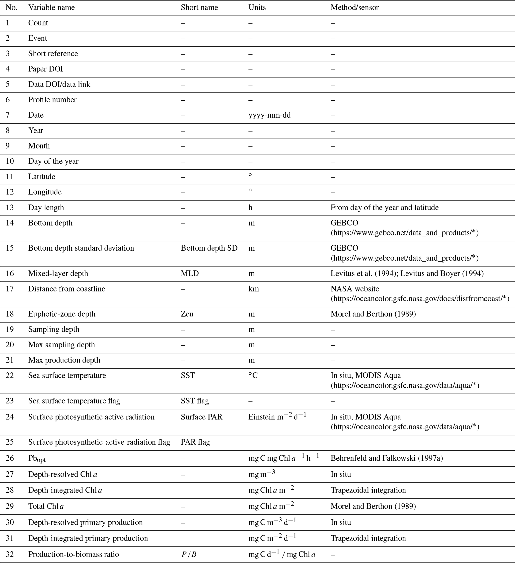
the Creative Commons Attribution 4.0 License.
 | 27 Oct 2021
Collection and analysis of a global marine phytoplankton primary-production dataset
Francesco Mattei
Michele Scardi
Phytoplankton primary production is a key oceanographic process. It has relationships with marine-food-web dynamics, the global carbon cycle and Earth's climate. The study of phytoplankton production on a global scale relies on indirect approaches due to the difficulties of field campaigns. Modeling approaches require in situ data for calibration and validation. In fact, the need for more phytoplankton primary-production data was highlighted several times during the last decades.
Most of the available primary-production datasets are scattered in various repositories, reporting heterogeneous information and missing records. We decided to retrieve field measurements of marine phytoplankton production from several sources and create a homogeneous and ready-to-use dataset. We handled missing data and added variables related to primary production which were not present in the original datasets. Subsequently, we performed a general analysis highlighting the relationships between the variables from a numerical and an ecological perspective.
Data paucity is one of the main issues hindering the comprehension of complex natural processes. We believe that an updated and improved global dataset, complemented by an analysis of its characteristics, can be of interest to anyone studying marine phytoplankton production and the processes related to it. The dataset described in this work is published in the PANGAEA repository (https://doi.org/10.1594/PANGAEA.932417) (Mattei and Scardi, 2021).
- Article
(3893 KB) - Full-text XML
- BibTeX
- EndNote


Phytoplankton primary production is a pivotal process in biological oceanography. It accounts for roughly 98 % of marine-system autotrophic production and 50 % of global productivity (Carvalho et al., 2017; Field et al., 1998). Accordingly, this process provides the main source of energy for structuring the marine food webs (Duarte and Cebrián, 1996; Kwak and Park, 2020a). Furthermore, it influences the absorption of carbon dioxide from the atmosphere and the flux of carbon to the deep ocean, generating a process known as biological pump (Giering et al., 2014; Longhurst and Glen Harrison, 1989). The estimated global phytoplankton production is comprised of between 30 and 70 Gt C yr−1 (Carr et al., 2006; Friedrichs et al., 2009; Saba et al., 2010; Siegel et al., 2013), i.e., most probably still larger than global anthropogenic CO2 emissions (roughly 37 Gt CO2 yr−1) (Caldeira and Duffy, 2000; Falkowski and Wilson, 1992; Jackson et al., 2019; Peters et al., 2020; Sabine et al., 2004).
These features highlight the strong link between phytoplankton production and both ecosystem services and Earth's climate (Barange et al., 2014; Behrenfeld et al., 2006; Blanchard et al., 2012a; Blythe et al., 2020). This link in turn reflects the central role of this biological process not only in the oceans' dynamics but also in those of the whole geobiosphere.
The availability of remotely sensed information allowed for the study of phytoplankton production at a global scale, providing a synoptic view of several ocean features, such as chlorophyll a surface concentration, sea surface temperature (SST) and photosynthetic active radiation (PAR) (Groom et al., 2019; Platt and Sathyendranath, 1988; Sammartino et al., 2018; Westberry and Behrenfeld, 2014). Several models which exploit satellite information to estimate primary production have been proposed (e.g., Behrenfeld and Falkowski, 1997; Friedrichs et al., 2009; Mattei and Scardi, 2020; Westberry and Behrenfeld, 2014). In fact, estimators of this process provide valuable tools to assess characteristics and patterns of global phytoplankton production, which in turn could provide insights into the dynamics of several phenomena, e.g., fishery yields and climate change effects (Fox et al., 2020; Richardson and Schoeman, 2004; Russo et al., 2019).
Nevertheless, the lack of field data negatively affects the power and the reliability of both satellite information and model estimates. In fact, these data are essential to calibrate satellite sensors and develop primary-production estimators.
The most complete and freely accessible phytoplankton production dataset is available at http://sites.science.oregonstate.edu/ocean.productivity/field.data.c14.online.php (last access: 26 January 2020). From now on we will refer to these data as the Ocean Productivity dataset. This dataset contains data from several oceanographic cruises accounting for roughly 3000 production profiles. Accordingly, this dataset has been widely used to develop several models (Behrenfeld and Falkowski, 1997; Scardi, 2001), since it contains depth-resolved 14C phytoplankton production estimates coupled with chlorophyll a profiles, SST and PAR measurements. Such data are crucial for both studying phytoplankton production and developing models for estimating this process. Despite being a precious source of information, these field data cover only some ocean basins, are affected by missing values and have not been updated since 1994 (orange dots in Fig. 1). As the amount and quality of field data are paramount characteristics to understanding the dynamics of natural processes, we wanted to create a new global dataset expanding both the temporal and the spatial coverage of the previously cited one. Moreover, we decided to associate more production-related information to each record, e.g., production-to-biomass ratio, bottom depth of the sampling station, distance from the coastline, etc. The extra information could be extremely valuable for analysis and modeling purposes, especially when machine-learning techniques come into play (Peters et al., 2014; Recknagel, 2001).
In order to retrieve phytoplankton production data, we consulted several sources which provide freely accessible information such as PANGAEA, the Biological and Chemical Oceanography Data Management Office and the National Centers for Environmental Information (a complete list of the exploited datasets with their respective references can be found in the Supplement).
To select suitable data, we adopted only four compulsory criteria that the newly found information had to meet. The first two criteria were related to the spatiotemporal context of the observations. Accordingly, we kept only the data for which date (yyyy-mm-dd) and geographical coordinates (latitude and longitude) of the field measurements were recorded. The third fundamental requirement was the presence of depth-resolved 14C measurements, i.e., phytoplankton production profiles. Depth-resolved data are more informative with respect to the depth-integrated ones, since they provide information not only on the production magnitude but also on its vertical distribution. The final requirement was the measurement of chlorophyll a profiles associated with the production data. Chlorophyll a is the most abundant pigment in photosynthetic organisms, and it is responsible for light energy absorption. The concentration of this pigment is intimately related to phytoplankton productivity, i.e., the production of organic matter. In fact, the energy gathered from sunlight allows for fixing carbon dioxide into matter. Even if several studies suggest that the chlorophyll-to-carbon ratio could be extremely variable depending on physical forces and phytoplankton physiological adaptation (Huot et al., 2007; Westberry et al., 2008), chlorophyll a is one of the most commonly used proxies for phytoplankton biomass, which in turn is a key parameter for studying phytoplankton production. This is especially true when the relationship between the pigment and the biomass is not explicitly formulated, i.e., in the machine-learning field. Furthermore, chlorophyll a can be easily measured with probes during sampling cruises, and its surface concentration has also been estimated from remote-sensing platforms since 1978 thanks to the Coastal Zone Color Scanner (CZCS). The former feature is important to exploit these measures to develop production models, while the latter is crucial in a synoptic application of these estimators.
On the other hand, we did not discard records lacking other variables, such as SST or PAR. In fact, if these measurements were not available, we filled the gaps by using interpolation techniques or retrieving the missing information from satellite platforms (see Sect. 2.1).
Retrieving phytoplankton production data that were not present in the Ocean Productivity dataset and the gap-filling operation allowed for expanding both the spatial and the temporal coverage of this dataset. Spatial and temporal variability are important features in dealing with global assessments of natural processes such as phytoplankton primary production. The new dataset comprised 6084 production profile collected between 1958 and 2017, 2214 of which derived from the Ocean Productivity dataset. The need for a larger amount of data related to the phytoplankton production process was already highlighted by several studies which either developed or compared primary-production models (Campbell et al., 2002; Carr et al., 2006; Friedrichs et al., 2009; Lee et al., 2015; Saba et al., 2010; Scardi, 1996). In fact, from the latter type of studies emerged a high level of uncertainty in determining global phytoplankton production. The range of estimated global production which resulted from comparison papers was extremely large, highlighting how challenging modeling this process on a large scale could be.
Additionally, we enriched the new dataset with several qualitative and quantitative variables. These variables were either derived from the existing one, retrieved from satellite platforms or extracted from freely accessible dataset (see Sect. 2.2).
Once the new dataset was structured, we highlighted its characteristics using several descriptive techniques and analyzed the results from an ecological perspective (Sect. 3).
2.1 Data merging and reconstruction
As stated in the previous section, the most complete dataset of phytoplankton primary production was freely downloadable from the Ocean Productivity website. It contained roughly 3000 production profiles (Fig. 1, orange dots) associated with ancillary information such as chlorophyll profiles, SST and PAR measurements. We used this dataset as starting point and searched for data that could improve its spatial and temporal coverage. We conducted our searches mainly on the PANGAEA and NOAA websites, which are freely accessible data repositories. Each dataset that we used in this work has been cited as specified by the repository or the owners (see Supplement). We limited our search to datasets which contained depth-resolved measurements of net phytoplankton production such as 14C associated with the respective chlorophyll a concentration. The main reasons for this choice were the additional vertical distribution information provided by phytoplankton profiles with respect to depth-integrated estimates and the biomass proxy provided by the chlorophyll concentration. This feature allowed for analyzing several characteristics of phytoplankton production, thus contributing to a deeper understanding of the whole process.
The retrieved data were incorporated into the new dataset only if the geographic coordinates and the sampling date had been recorded. These data allowed for accounting for both the spatial and temporal variability of phytoplankton production in the analysis.
For each retrieved dataset that met our requirements, the first step was to merge it with the Ocean Productivity one. From the latter dataset we kept the following variables: date of the sampling (yyyy-mm-dd), geographical coordinates of the sampling station (latitude and longitude and degrees), day length as hours of the photoperiod (h), sampling depth (m), Pbopt (mg C mg Chl a−1 h−1), SST (∘C), surface PAR (Einstein m−2 d−1), sampling depth chlorophyll a concentration (mg m−3), sampling depth daily primary production (mg C m−3 d−1) and integrated daily primary production (mg C m−2 d−1). To perform the merging procedure, we filled all the gaps in the newly retrieved data relative to the abovementioned variables. We computed the day length from the latitude and the day of the year of the sampling. SST missing values were filled using MODIS daily data for observations from 2003 to the present (MODIS Aqua Mapped Daily 4 km (https://doi.org/10.5067/MODSA-1D4D9, NASA OBPG, 2020), multiple-sensor daily data for records from 1981 to 2003 and the 1981–1990 mean for the data prior to 1981 (Copernicus SST) (Merchant et al., 2019). We also used the MODIS values for filling the PAR gaps from 2003 to the present. The profiles previous to this date that lacked PAR measures were discarded, since daily PAR estimates are available only through the MODIS platform (late 2002 to the present). Discarding these data, the Ocean Productivity dataset dropped from roughly 3000 profiles to 2214. We estimated the Pbopt parameter using the procedure proposed by Behrenfeld and Falkowski (1997a). Finally, we estimated the missing values in chlorophyll a and primary-production profiles with a depth-weighted average of adjacent values. Once the merging procedure was finished, the new dataset contained 37 722 records from 6084 profiles with respect to the 14 300 and 2214 of the old one (Fig. 1).

Figure 1Map of the 6084 phytoplankton production profiles comprised in the new dataset. In orange are the profiles derived from the Ocean Productivity dataset (2214), and in red are the newly retrieved ones (3870).
2.2 Ancillary data association
We added several variables related to phytoplankton primary production to the dataset (Tables 1 and 2). These variables can be divided into three groups: (i) data extracted from freely available datasets, (ii) numerical measures computed from the existing ones and (iii) categorical data derived from the previous two groups.
Among the variables that belong to the first group, we list the bottom depth (m) and the statistics related to it. We retrieved the bathymetry information from the GEBCO website (General Bathymetric Chart of the Oceans; https://doi.org/10.5285/c6612cbe-50b3-0cff-e053-6c86abc09f8f, GEBCO Compilation Group, 2021). We queried the GEBCO dataset using the geographic coordinates of the sampling stations to extract the bottom depth data. We also exploited up to eight neighbor pixels to compute the bottom depth variance of the sampling-point neighborhood.
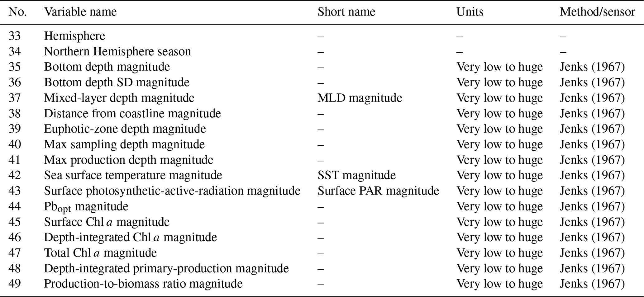
We retrieved information about the mixed-layer depth (MLD) using the Levitus model datasets (Levitus et al., 1994; Levitus and Boyer, 1994), which are freely available on the Levitus web page (https://psl.noaa.gov/data/gridded/data.nodc.woa94.html, last access: 26 January 2020, NOAA/OAR/ESRL PSL, 2021)
The last data that we gathered from an external dataset were the distance from the coastline (km). The 0.04 ∘ distance dataset was downloaded from the NASA website (https://oceancolor.gsfc.nasa.gov/docs/distfromcoast/, NASA Ocean Biology Processing Group (OBPG) and Stumpf, 2012).
The second group of new variables was computed from information already present in the new production dataset at this stage. We computed the day of the year from the date, i.e., the first day of January and the last day of December were represented by 1 and 365 respectively.
Table 1Production dataset numerical variables.
* last access: 26 January 2020.
We also estimated the euphotic-zone depth and the total chlorophyll a in the euphotic zone (mg Chl a m−2) using a model developed by Morel and Berthon (1989).
Moreover, we extracted both the max sampling depth of non-null production values (m) and the depth at which maximum production occurred for each profile (m), thus creating two new variables.
We estimated depth-integrated chlorophyll a and depth-integrated primary production (IPP) by the trapezoidal integration of in situ measurements (mg Chl a m−2 and mg C m−2 d−1 respectively). Subsequently, we estimated the production-to-biomass ratio by dividing the depth-integrated phytoplankton production by the depth-integrated chlorophyll a concentration (mg C d−1 mg Chl a).
The last group of variables were generated by dividing the production profiles in classes on the basis of the previously computed variables. We created the hemisphere variable by assigning each profile to the Northern Hemisphere, Southern Hemisphere or Equator on the basis of the sampling latitude. We also created a season variable on the basis of the date and Northern Hemisphere season. We divided the year into four groups of 3 months each starting from January and tagged them as winter, spring, summer and fall respectively.
For numerical data, we applied the Jenks optimization algorithm (Jenks, 1967) to define the boundaries of six classes from very low to huge (very low, low, moderate, high, very high and huge). Then we used these boundaries to assign each pattern to one of the six classes. It is important to note this class segmentation is relative to our data rather than an absolute classification criterion. Finally, we added two columns to provide information about the nature of the SST and PAR measures. These flag columns specify if the variable's value is either in situ (flag value = 0) or reconstructed (flag value = 1), and these are placed near the flagged variable.
Finally, we investigated the relationship between the variables which are more intimately related to phytoplankton primary production, i.e., SST, PAR, chlorophyll a, max sampling depth, max production depth and the production-to-biomass ratio. We produced heatmaps to provide an insight into the categorical variables and performed a principal-component analysis (PCA) for their numerical counterparts.
With this work we aimed at building a global phytoplankton production dataset updating the Ocean Productivity one. Moreover, we wanted to expand the available information by associating several variables related to primary production. The data underlying this article are available in the article's online Supplement.
The comprehension of natural phenomena deeply relies on available data. These complex processes often involve nonlinear and not well-known relationships among their components. Accordingly, we believe that one crucial way to enhance our understanding of natural systems is provided by gathering information and then analyzing it.
In this framework, we extended both the spatial and the temporal coverage of the Ocean Productivity dataset. These two features are paramount to boosting our knowledge about the spatiotemporal distribution of phytoplankton production. In fact, the former allows for taking temporal trends into account in the processes which are linked with climate-related issues and food web dynamics. The Ocean Productivity dataset contained data from cruises carried out between 1958 and 1994, which is a large span of time, but it has not been updated since then. Our data retrieval added 23 422 new patterns from 3870 production profiles which in most cases do not overlap with the Ocean Productivity dataset's temporal coverage. In fact, 2210 of the 3870 new phytoplankton profiles, i.e., roughly 57 % of the total, were collected between 1995 and 2017. Even if roughly 43 % of the new profiles share the time coverage with the Ocean Productivity ones, the majority of these data do not overlap with the spatial coverage of the older dataset, thus enhancing the heterogeneity of the data.
Although the Ocean Productivity dataset was the most comprehensive source of information about phytoplankton primary production, the bulk of its data were restricted to three main regions. These areas were the northwestern Atlantic, the eastern equatorial Pacific and the northeastern Pacific along the western coast of the United States. The other ocean basins were undersampled or not sampled at all (Fig. 1, orange markers). The new data improved the global coverage of the previous dataset. Several profiles were added in the Arctic Ocean, specifically in the Chukchi Sea, the Beaufort Sea, the Greenland Sea, the North Sea, the Norwegian Sea, the Barents Sea and the Kara Sea. In the Pacific Ocean the newly represented areas were the Bering Sea, the Gulf of Alaska, and the areas off of the Oregon and California coasts in addition to a few production profiles gathered off the eastern coast of New Zealand. In the western Atlantic, new information was available for the Gulf of St. Lawrence, the Florida coast and the Caribbean Sea. In the central Atlantic the newly represented areas were located southeast of Ireland, south of Cabo Verde and off of the Gulf of Guinea with a few records in the Bay of Biscay, off of the coast of Morocco and in the Mediterranean Sea. Few of the data in the Indian Ocean were present in the old dataset, but we reconstructed missing information and added new profiles from different datasets. The Southern Ocean remains strongly undersampled, with the addition of a few production profiles.
The temporal and spatial coverage of a dataset are crucial features. The first one allows for taking the evolution of the studied process into account. This aspect is important in any type of assessment work, especially in a climate change context. In the phytoplankton production framework, the temporal span covered by the available in situ data could be used to study several aspects. For example, repeated observations through the years for the same area could highlight temporal patterns of the investigated region. Moreover, this feature could be used to investigate the relationships between phytoplankton production and large-scale phenomena, e.g., El Niño–Southern Oscillation (ENSO). From a spatial perspective, the larger the global oceans area represented in the dataset is, the larger the spatial variability of the phytoplankton production process taken into account is. This feature is crucial, since both depth-resolved and depth-integrated phytoplankton production estimates are deeply influenced by the geographic characteristics of the investigated area, e.g., latitude, distance from the coastline and bottom depth. Therefore, to deepen the understanding of this biological process, we need to gather and analyze information from different areas. Finally, if we want to exploit a dataset to perform any global assessment of the phytoplankton primary production or tackle production-climate-related issues, we need an information pool that takes into account as much variability of the process as possible (Behrenfeld et al., 2016; Gibert et al., 2018; Hays et al., 2005).
One of the fields which heavily relies upon the amount and quality of the data is modeling. Several studies stressed how most of the limits in modeling phytoplankton production depend upon the data availability (Campbell et al., 2002; Carr et al., 2006; Mattei and Scardi, 2020; Scardi, 2001). For these reasons, we believe that the enhancement of both spatial and temporal coverage of a freely available production dataset is an important contribution to modern oceanography.
Not only did we limit our work to homogenize several data sources into a single one, but also we enhanced the amount of phytoplankton-related available information. This type of information could be useful for boosting our understanding of primary production. Moreover, the ancillary data could be extremely valuable to model development, especially when machine-learning techniques come into play. In fact, these approaches allow for the use of variables as predictors even if the relationship with the target variable (primary production here) is not known (Catucci and Scardi, 2020; Franceschini et al., 2019; Olden et al., 2008; Peters et al., 2014; Recknagel, 2001).
The first two descriptors added to the new dataset were the hemisphere of the sampling station and sampling season, indicated as the Northern Hemisphere season. These two variables provided an insight into the global temporal and spatial distribution of the data (Fig. 2).
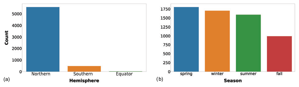
Figure 2(a) Number of profiles gathered in the two hemispheres or at the Equator (5578, 478 and 28 respectively). (b) Number of profiles sampled in Northern Hemisphere winter (January to March), spring (April to June), summer (July to September) and fall (October to December).
The spatial distribution of the records was strongly unbalanced towards the Northern Hemisphere compared to the Southern Hemisphere (5578 vs. 478 production profiles, Fig. 2a). This feature highlights the importance of gathering more data in the Southern Hemisphere. In particular, the Southern Ocean is one of the least well-known areas of the global ocean, and the uncertainty related to this lack of knowledge negatively affects our understanding of both global phytoplankton production and the carbon cycle (Arrigo et al., 2008; Caldeira and Duffy, 2000; Moigne et al., 2016; Reuer et al., 2007).
On the other hand, the temporal variability in the new dataset is more balanced with respect to the spatial one. Accordingly, the number of profiles sampled during the Northern Hemisphere winter, spring, summer and fall are respectively 1701, 1802, 1589 and 992. This is an important feature, especially for the areas characterized by seasonal patterns which influence not only the magnitude of primary production but also its distribution along the water column (Falkowski and Raven, 2007a). Therefore, when both the depth-integrated and the depth-resolved perspectives are taken into account, this temporal variability is doubly valuable.
We also added information related to the bathymetry of the sampling area. We queried the GEBCO dataset to extract the bottom depth of sampling stations. Afterwards, we applied the Jenks optimization algorithm to partition the data into six classes (Fig. 3).
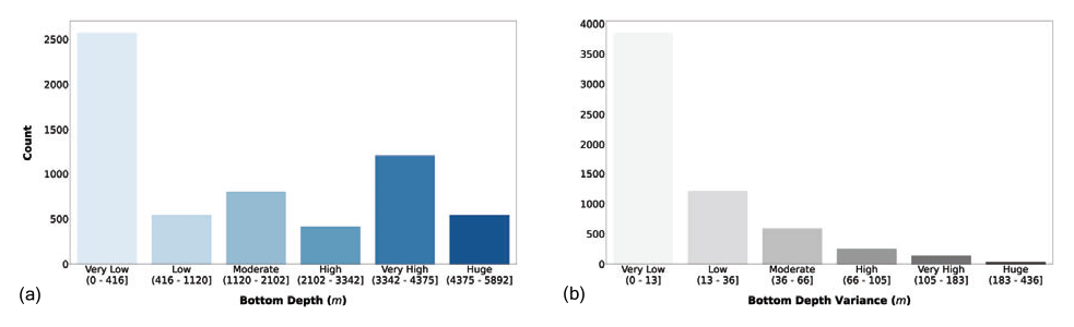
Figure 3(a) Bottom depth and (b) its variance classes. The bar color intensity reflects the magnitude of the class values.
The majority of the observations were collected in areas shallower than 416 m (Fig. 3a). This feature highlights that the continental-shelf areas are the most frequently sampled ones. The second class in terms of abundance was the very high one, while the other classes had less than 1000 profiles each. In Fig. 3b we can notice that almost all the sampling stations had a very low bottom depth variance in their neighborhood; thus the area of the sampling was homogenously deep. Bathymetry-related information could help in understanding the geomorphological region of the ocean where the sampling station was situated, i.e., coastal, continental shelf or open ocean.
The depth information could help us analyze the profiles' characteristics, since it could be interpreted as a proxy for several features such as nutrient availability and water column dynamics. In fact, even if the depth is not directly related to phytoplankton production, it is an important physical descriptor of the ocean system in which this biological process occurs.
The MLD data were retrieved from the Levitus dataset. These estimates provide a seasonal indication for the water column mixing status, which is related to both the magnitude and the vertical distribution of phytoplankton production. We also added the distance from coastline as ancillary information. This distance provides an insight into how many factors like terrestrial runoff, rivers and waste water discharges could affect the primary production. It is well known that coastal areas are characterized by higher levels of primary production mainly due to nutrient inputs from natural and anthropogenic sources (Paerl et al., 1990; Teixeira et al., 2018; Wollast, 1998).

Figure 4(a) MLD (m) and coastal-distance (km) magnitude. The bar color intensity reflects the magnitude of the class values.
Figure 4a shows that 96.4 % of the sampling stations presented a very low to moderate MLD. The distance from the coastline showed the same pattern with the bulk of the profiles comprising the first two classes (Fig. 4b). The main reason for adding these variables to our dataset is their relationship with nutrient availability which generally became scarcer as the distance from the coastline and the bottom depth augment. Moreover, the available nutrients are distributed in different concentrations along the water column according to the MLD magnitude (Falkowski and Raven, 2007a; Huisman and Weissing, 1995; Jäger et al., 2008). The latter feature is one of the factors influencing the vertical distribution of phytoplankton production.
Another group of variables was extracted directly from the sampling data. We created the maximum sampling depth as the depth at which the deepest water sample was collected (Fig. 5a). Usually, this depth corresponds to the 1 % of the surface irradiance, but it was not specified in all the retrieved data. We also introduced the maximum production depth, which is the depth where the maximum depth-resolved production value occurred, i.e., the peak of the production profile (Fig. 5b).

Figure 5(a) Maximum profile depth and (b) maximum production depth classes. The bar color intensity reflects the magnitude of the class values.
The majority of the records showed very low to high production profile depth. In fact, these four classes included 94.3 % of the records. Among these classes the most represented was the very low one (to 33 m). This feature reflected again the higher number of coastal profiles with respect to the open-ocean ones. The profile peak depth showed an even stronger decreasing trend with respect to profile depth. In fact, 76.7 % of the patterns were characterized by a peak in the first two classes. The decrease in primary production with depth is mainly justified by the light attenuation along the water column, which is one of the main physical forces influencing phytoplankton production. In fact, even if deeper waters are usually nutrient rich, while the shallower ones are nutrient depleted, the photosynthetic process cannot prescind from light availability.
SST and surface PAR variables were already present in the Ocean Productivity dataset but showed several missing data. As described in the Sect. 2.1, we filled the gaps where possible in both the old and the new data. The results of the Jenks algorithm on SST and PAR variables are presented in Fig. 6.

Figure 6(a) Sea surface temperature and (b) photosynthetic-active-radiation classes. The bar color intensity reflects the magnitude of the class values.
SST and surface PAR showed different patterns with respect to the previously discussed variables. The bulk of the records showed moderate values of SST (roughly 50 % of the production profiles), while the lowest and highest values were the least abundant. The surface PAR classification showed a different pattern in which the very low values were the majority followed by the very high and the huge values.
These two parameters exert an important influence on phytoplankton primary production, and they have been key factors in modeling this biological process. In fact, SST affects physiological characteristics of phytoplankton, influencing its primary productivity, and PAR represents the share of solar energy that is used for CO2 fixation.
Unfortunately, most of the time these parameters are measured only at surface level, while it could be extremely useful to have depth-resolved in situ measurements for studying phytoplankton production from a depth-resolved perspective.
One of the most important variables related to phytoplankton production is the depth-resolved chlorophyll a concentration. It was one of the compulsory requirements for inclusion in the gathered dataset. Even if the relationship is not straightforward, it is often used as phytoplankton biomass proxy. Several works pointed out that other variables could be a more precise proxy (Huot et al., 2007; Westberry et al., 2008), but it is often difficult if not impossible to compute them for old data, thus limiting the effectiveness of the new candidates.
Starting from the chlorophyll a profiles, we also computed the depth-integrated values using a trapezoidal integration. We exploited the depth-integrated value to compute a production-to-biomass ratio and as source of information for the dataset analysis.
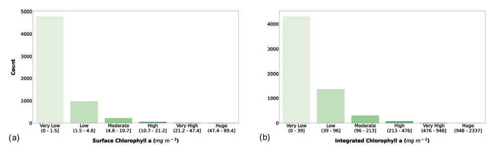
Figure 7(a) Surface chlorophyll a and (b) depth-integrated chlorophyll a classes. The bar color intensity reflects the magnitude of the class values.
The classification of surface chlorophyll a concentration (Fig. 7a) showed that 78.7 % of the phytoplankton profiles in the dataset fell in the very low class, and the first three classes comprised 98.5 % of the records. Surface chlorophyll a concentration is one of the main variables used to predict phytoplankton production, since it is related to the biomass of these autotrophic organisms. Moreover, this variable is retrievable through remote-sensing platforms, thus allowing for a quasi-synoptic application of production estimators.
The segmentation of the integrated chlorophyll a concentration (Fig. 7b) showed a similar pattern compared to the surface one. In fact, the first three classes were the most abundant (98.2 %), but Fig. 7b shows a larger number of low and moderate values than Fig. 7a (27.4 % vs. 19.8 %).
We considered the availability of phytoplankton production profiles as compulsory information for the newly retrieved data. The reason for this requirement was twofold: firstly, we wanted to keep all the information already present in the Ocean Productivity dataset, which contained depth-resolved measurements of phytoplankton production. Secondly, we believed that the study of phytoplankton production could benefit from the coupled information of magnitude and its distribution along the water column while only taking the former into account. Starting from the depth-resolved production data (mg C m−3 d−1), we computed the depth-integrated production using a trapezoidal integration (mg C m−2 d−1). Subsequently, we computed a production-to-biomass ratio using depth-integrated phytoplankton production and depth-integrated chlorophyll a. The segmentation in classes of IPP and production-to-biomass ratio is shown in Fig. 8.
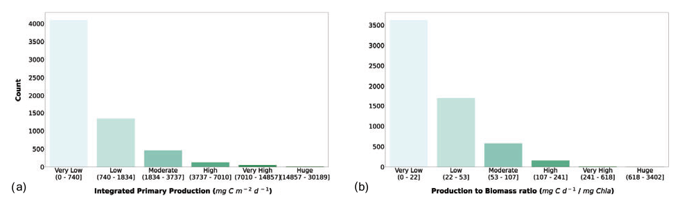
Figure 8(a) Depth-integrated phytoplankton primary production and (b) production-to-biomass ratio classes. The bar color intensity reflects the magnitude of the class values.
Both IPP and production-to-biomass ratio classifications showed the same pattern. Accordingly, the larger the class values are, the lower the numerosity of the class is. The first class comprised 67.3 % and 59.5 % of the profiles for IPP and the production-to-biomass ratio respectively.
IPP is an important measure in global assessments of phytoplankton production. It provides a bidimensional view (latitude vs. longitude) of the oceanic production, which in turn influences several biological and non-biological processes in the biosphere, e.g., energy flow into the marine food webs, fish landings and CO2 absorption (Anderson et al., 2018; Barange et al., 2014; Blanchard et al., 2012b; Caldeira and Duffy, 2000; Carvalho et al., 2017; Kwak and Park, 2020b; Maureaud et al., 2017; Shurin et al., 2006). On the other hand, depth-resolved production provides more insights into the phytoplankton production process characteristics, which in turn could lead to better estimates of IPP (Mattei et al., 2018).
The production-to-biomass ratio could convey valuable information about the physiological state of the phytoplankton, which in turn is influenced by biotic and abiotic forcing. This ratio can be also used to further analyze the profiles' characteristics and to decide whether they are suitable or not for specific purposes, e.g., modeling phytoplankton primary production (Mattei and Scardi, 2020; Scardi, 2001).
Subsequently, we selected a subset of these variables and described their relationships with the depth-integrated phytoplankton production (see heatmaps, Figs. 9–15).
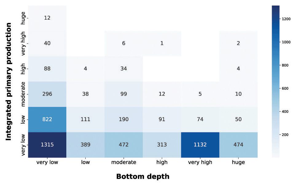
Figure 9IPP vs. bottom depth. The blue heatmap highlight the difference in production potential between coastal and open-ocean areas.
In the integrated production vs. bottom depth, the very low production class was the most abundant in all the depth ranges (Fig. 9). This feature was prominent in the very low and very high bottom depth classes, which comprised roughly 60 % of the very low production profiles. In very shallow areas the production could be limited to a small portion of the water column, thus often resulting in low integrated production values. On the other hand, open-ocean areas are usually nutrient depleted; thus phytoplankton production is limited even if other environmental conditions are favorable. Shallower sampled areas showed higher levels of depth-integrated production. This was manifest for the very low class, which showed a noticeable amount of profiles for each production class and the bulk of largest depth-integrated values, i.e., 67.7 %, 81.6 % and 100 % of the high, very high and huge production profiles respectively. The latter feature was mainly due to land inputs to coastal areas which, when associated with favorable physical conditions, lead to high production levels. The blue heatmap highlighted the high potential of shallower areas in contrast with the low one of the open-ocean zones.
The grey heatmap complement the information of the blue one by taking into account the local variance of the bottom depth (Fig. 10).
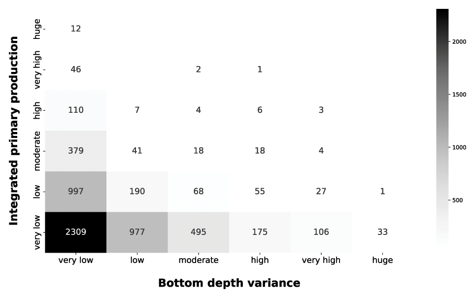
Figure 10IPP vs. bottom depth variance. The grey heatmap shows the relationship between the variance of the bottom depth and the IPP.
The very low bottom depth variance comprises the both very low and huge production profile. The low level of variance characterizes coastal areas, in which bottom depth is consistently low, and the open-ocean zones, in which the bottom depth was consistently high. Progressively larger variance values showed the transition from shallower to deeper areas, which corresponds to a decrease in depth-integrated production. This is consistent with our previous analysis and with phytoplankton ecology.
Subsequently, we analyzed the relationship between integrated production and the profile depth (Fig. 11).
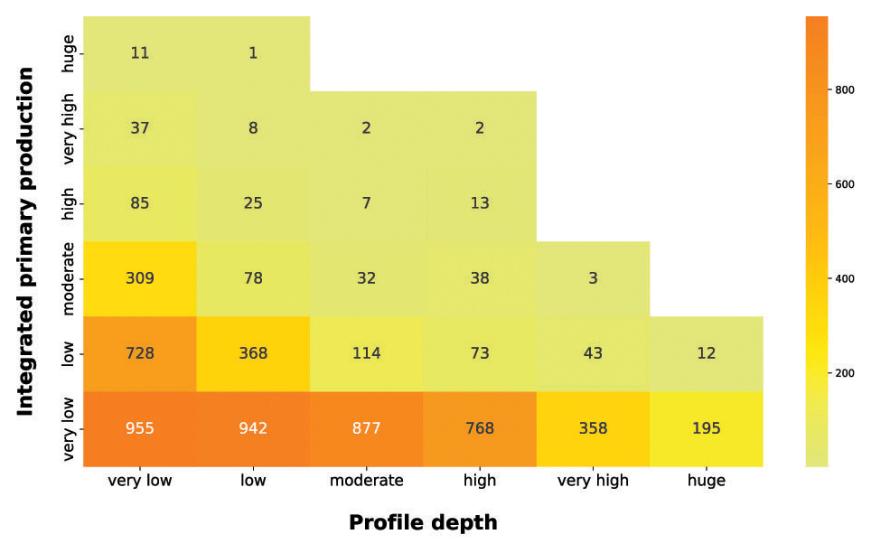
Figure 11IPP vs. profile depth. The yellow-to-orange heatmap highlights the relationship between the depth-integrated phytoplankton production and the production profile depth.
The yellow-to-orange heatmap showed that the bulk of high production profiles were in the first two profile depth classes. Shallow production profiles are usually the ones closer to the coastline or upwelling zones. These areas are nutrient rich even in surface waters, where light availability is high, thus allowing for a high level of production. Moreover, high levels of production in shallow waters enhance the light attenuation phenomenon, reducing the column water area suitable for primary production. Conversely, the deeper the phytoplankton profile is, the lower the depth-integrated production is. Low-nutrient conditions lead to low phytoplankton biomasses values and thus to a deeper light penetration along the water column. The latter feature allows for the structuring of deeper production profiles. Although these profiles occupy a large portion of the water column, the total profile production is limited by the scarce nutrient level.
Continuing our analysis of the relationship between depth-resolved features and the magnitude of depth-integrated production, we took into account the production peak depth (Fig. 12).
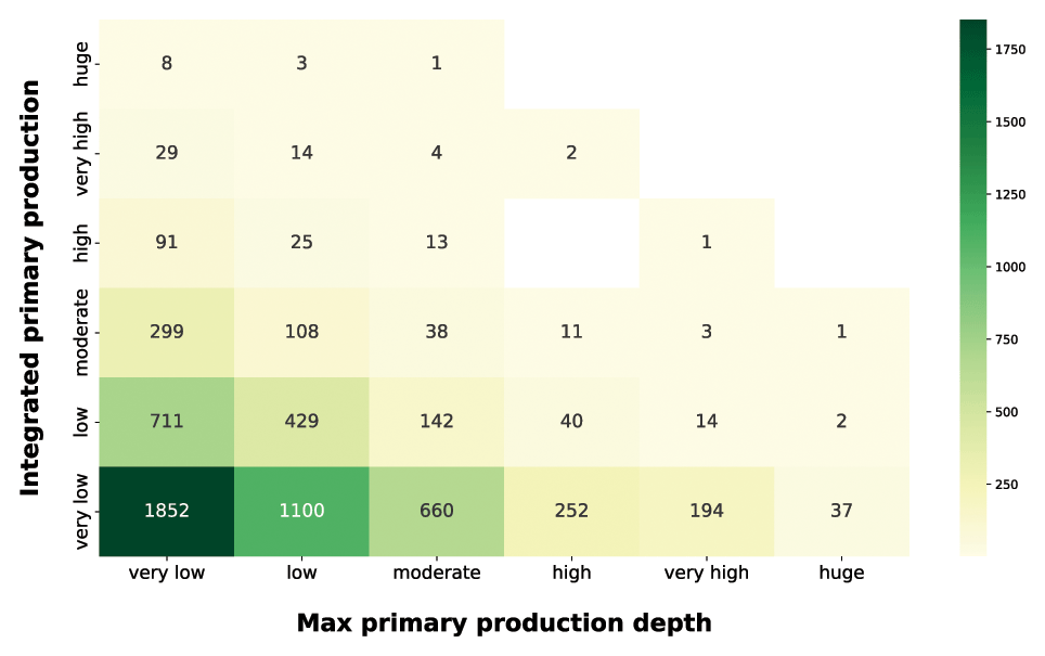
Figure 12IPP vs. maximum primary-production depth. The yellow-to-green heatmap shows how the magnitude of IPP is related to the depth at which the maximum production occurs.
The production distribution along the water column is influenced by physiological and physical forcing. The optimum between light and nutrient availability determines the depth at which the maximum production occurs (Falkowski and Raven, 2007b). Since light availability exponentially decreases with depth, shallow peaks reflect either a condition of low irradiance or high irradiance and high nutrients. Both of these situations lead to surface production peaks which are associated with a wide range of integrated-production magnitudes. The yellow-to-green heatmap highlighted how the high depth-integrated magnitudes are associated only with shallow-peak profiles. This feature reflected the relationship between phytoplankton physiological needs and the light extinction behavior. Deep production peaks indicate a nutrient paucity condition in shallow waters which shifts the optimum condition near the nutricline depth. From the integrated-production perspective, low values were associated with shallow peaks in conditions of low PAR or low nutrients even in deeper areas of the water column. The highest levels of production were coupled with surface or subsurface peaks, while deeper peaks (high to huge) represented 9 % of the total profiles and showed only very low to moderate depth-integrated production with the exception of three production profiles.
Among the physical forcing that influences phytoplankton production, we explored the characteristics of SST and PAR (Figs. 13 and 14). It is worth stressing that the segmentation derived from the Jenks algorithm is relative to our data. For instance, the procedure was influenced by the underrepresentation of circumpolar areas, especially in the colder months.
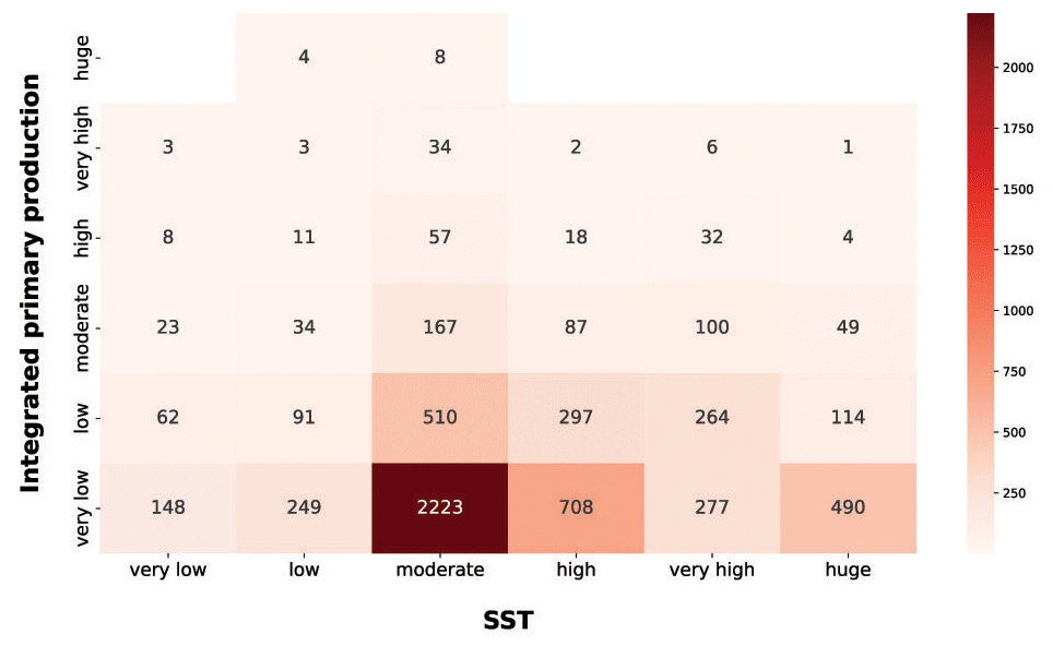
Figure 13IPP vs. SST. The red heatmap represents the relationship between depth-integrated production and SST.
The red heatmap showed that very low and low levels of SST were associated mainly with a low primary-production magnitude. The same pattern characterized very high and huge levels of SST. These features are related to primary-production seasonality induced by physical forcing. The former situation referred to cold seasons in which the nutrient levels in the water column is high but not enough solar radiation is available for the photosynthetic organisms. The latter reflects a strong shallow stratification of the water column which is typical of warm seasons or areas constantly subjected to high levels of irradiance. This leads to low nutrient concentration in shallow waters, which in turn severely limits the primary producers. Moderate levels of SST were associated with a wider range of values and comprised the larger levels of phytoplankton production. This feature could be associated with the transition between cold and warm seasons. In this period of the year the environmental conditions are optimal for primary production, since the high nutrient concentration accumulated during the cold season became exploitable due to the increasingly available solar radiation.
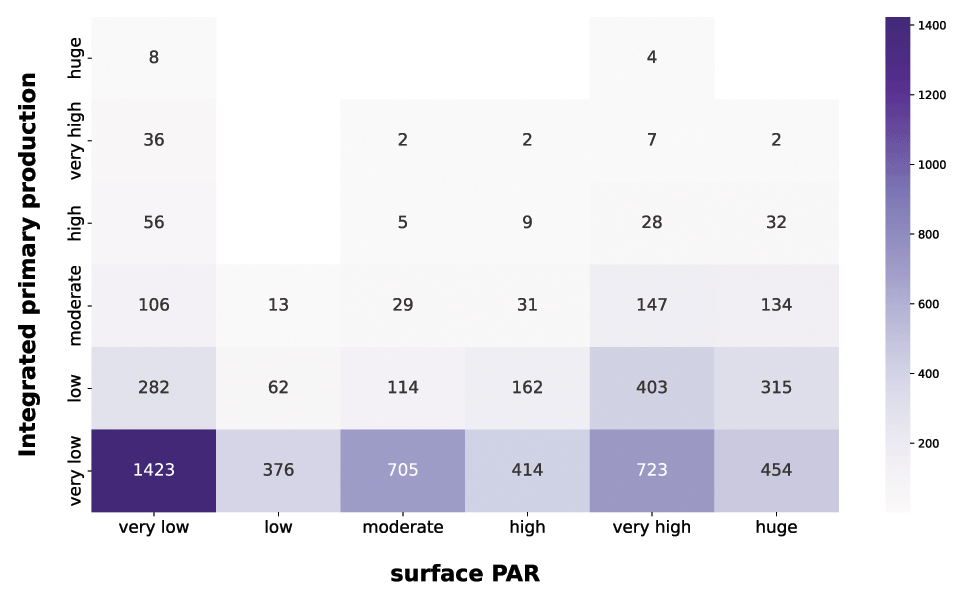
Figure 14IPP vs. PAR. The purple heatmap shows how integrated phytoplankton production and PAR are related to each other.
The first feature highlighted by the purple heatmap (Fig. 14) was the large share of very low integrated-production profiles in each PAR class. This is mainly related to the nutrient availability, since low nutrient concentration leads to very low production levels independently from the physical forcing.
Not surprisingly, very high and huge levels of PAR were associated with larger magnitudes of integrated production, since the photosynthesis is intimately related to the solar radiation.
Another striking aspect was the wide range of phytoplankton responses to very low PAR magnitudes. In fact, all the production levels are well represented in this PAR class, showing that the geographical characteristics of the area deeply influence the primary producers. Accordingly, a constant nutrient input from terrestrial runoff can boost the primary production especially in shallower layers of the water column where usually it is nutrient limited.
The last relationship that we analyzed was the one between IPP and depth-integrated chlorophyll a (Fig. 15).

Figure 15IPP vs. chlorophyll a. The green heatmap relates the depth-integrated phytoplankton production to the chlorophyll a magnitude, which is one of the most used proxies for phytoplankton biomass.
The pattern that emerged from the green heatmap (Fig. 15) was one proportional to moderate chlorophyll a values. Accordingly, the higher the integrated production is, the higher the integrated chlorophyll a is. The bulk of the profiles were comprised in the very low and low integrated chlorophyll a classes; 3992 profiles (65.6 % of the total patterns) from very low and low chlorophyll a concentration were coupled with very low production, while 1227 (20.1 % of the total patterns) were associated with low production. Conversely, higher levels of integrated chlorophyll a were characterized by a larger share of high production profiles. This was not surprising, since chlorophyll a is the principal photosynthetic pigment, and its raise is caused by physiological needs of phytoplankton or biomass augmentation.
The final analysis we carried out was a PCA to spot and analyze general patterns in the dataset. We selected the following 12 variables to perform the PCA: day length, bottom depth, bottom depth variance, MLD, distance from coastline, SST, PAR, surface chlorophyll a, integrated chlorophyll a, surface phytoplankton production, integrated phytoplankton production and the production-to-biomass ratio (Fig. 16).
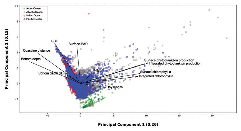
Figure 16Principal-component analysis of 0.26 and 0.15 explained variance from the first two axes respectively. The dimensionality reduction provided by the PCA allowed for the visualization of several data patterns despite the strong spatiotemporal variability of the dataset.
We used type one scaling, since our main focus was on the position of the profiles. Using this type of scaling the distance between the objects in the plot approximate their Euclidean distances in full-dimensional space. The variance explained by the first and the second axis was 0.26 and 0.15 respectively. The relatively low share of explained variance highlights the high complexity of the data which encompass large levels of spatial and temporal variability. Nevertheless, the ordination allowed for spotting and showing several features of the production dataset. From a general point of view high levels of surface and depth-integrated chlorophyll a are associated between them. The same remark is valid for phytoplankton production. Moreover, is not surprising that chlorophyll a concentration and phytoplankton production measures point in the same direction along the first axis. Another feature that is consistent with the results previously presented was the inverse relationship between bottom depth and coastline distance with respect to primary-production magnitude.
Since the various oceans showed different characteristics, we decided to analyze the PCA output also from each specific macro-area perspective (Fig. 17).
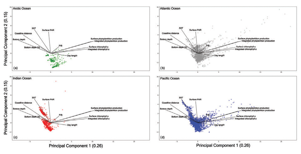
Figure 17Principal-component analysis results for each ocean. (a) The Arctic Ocean shows a condensed cloud of points highlighting the narrow range of recorded measures due to the peculiarity of this ocean. (b) The Atlantic Ocean presents the most dispersed cloud of points and the largest in situ measures of primary production. (c) The Indian Ocean shows two distinct groups of points which highlight how the monsoon system influences this area. (d) The Pacific Ocean is characterized by a wide range of sampled environmental and biological variables which depend on the large spatial extent of this basin and the considerable number of patterns gathered during the years.
The Arctic Ocean (Fig. 17a) presented the narrowest cloud of points among the basins. This could be the result of the low number of records collected in this region and the peculiar characteristics of the area which hinder the sampling procedures. The Arctic Ocean data are characterized by a low level of SST and PAR throughout the year with the exception of short periods of time.
The Indian Ocean showed two groups of samples. This feature was the result of the monsoon system that characterizes this basin. The wind blows from the northeast during cooler months and from the southwest during the warmest months of the year (Dickson et al., 2001). Moreover, the plot (Fig. 17c) shows that this is not a highly productive area independent from the environmental conditions. In fact, the bulk of the points were placed in the opposite direction of both chlorophyll a concentration and phytoplankton production levels.
A large amount of information was associated with the Atlantic Ocean and Pacific Ocean (Figs. 17b and d respectively), since they were the most sampled areas. Accordingly, they showed the largest range of sampled conditions with high and low levels for almost every environmental and biological variable. This feature is also influenced by the spatial extent of these two basins which cover a considerable portion of Earth's oceans. Moreover, almost every profile associated with a high level of phytoplankton production or chlorophyll a concentration was recorded in these basins that encompass highly productive areas including several upwelling zones.
The dataset described in this work is published in the PANGAEA repository (https://doi.org/10.1594/PANGAEA.932417) (Mattei and Scardi, 2021). A PDF file containing the supplementary data information is available in the data repository.
The data paucity is one of the most important issues related to several disciplines, and ecology is no exception. This is especially true if the task to tackle is understanding the dynamics of a complex biological process, such as phytoplankton primary production, on a global scale. Moreover, several researchers during the last decades highlighted how the lack of data is the main constraint for modeling phytoplankton production.
In this framework, we believe that building a new, homogenous and ready-to-use dataset, associated with a general analysis of its features, could play an important role in the study of phytoplankton production especially if combined with related and complementary published works (e.g., Kulk et al., 2020; Bouman et al., 2018). For this reason, we retrieved phytoplankton production data from heterogeneous sources and created a new global dataset. We also applied several data analysis and visualization techniques to spot and discuss both the dataset characteristics and the variables' relationships.
Furthermore, enriching the dataset with ancillary data related to phytoplankton production could be extremely useful in improving our understanding of this pivotal process, e.g., in a machine-learning context.
Despite the new dataset still being unbalanced from a spatial and temporal perspective and the need for new data never being fully satisfied, we believe that this dataset represents a crucial improvement on the previous ones.
FM collected, processed and analyzed the data. FM wrote the paper. MS supervised the project.
The contact author has declared that neither they nor their co-authors have any competing interests.
Publisher’s note: Copernicus Publications remains neutral with regard to jurisdictional claims in published maps and institutional affiliations.
This paper was edited by François G. Schmitt and reviewed by two anonymous referees.
Anderson, T. R., Martin, A. P., Lampitt, R. S., Trueman, C. N., Henson, S. A., and Mayor, D. J., Quantifying carbon fluxes from primary production to mesopelagic fish using a simple food web model, edited by: Link, J., ICES J. Mar. Sci., 76, 690–701, https://doi.org/10.1093/icesjms/fsx234, 2019.
Arrigo, K. R., van Dijken, G. L., and Bushinsky, S.: Primary production in the Southern Ocean, J. Geophys. Res. Oceans, 113, 1997–2006, https://doi.org/10.1029/2007JC004551, 2008.
Barange, M., Merino, G., Blanchard, J. L., Scholtens, J., Harle, J., Allison, E. H., Allen, J. I., Holt, J., and Jennings, S.: Impacts of climate change on marine ecosystem production in societies dependent on fisheries, Nat. Clim. Change, 4, 211–216, https://doi.org/10.1038/nclimate2119, 2014.
Behrenfeld, M. J. and Falkowski, P. G.: Photosynthetic rates derived from satellite-based chlorophyll concentration, Limnol. Oceanogr., 42, 1–20, https://doi.org/10.4319/lo.1997.42.1.0001, 1997.
Behrenfeld, M. J., O'Malley, R. T., Siegel, D. A., McClain, C. R., Sarmiento, J. L., Feldman, G. C., Milligan, A. J., Falkowski, P. G., Letelier, R. M., and Boss, E. S.: Climate-driven trends in contemporary ocean productivity, Nature, 444, 752–755, https://doi.org/10.1038/nature05317, 2006.
Behrenfeld, M. J., O'Malley, R. T., Boss, E. S., Westberry, T. K., Graff, J. R., Halsey, K. H., Milligan, A. J., Siegel, D. A., and Brown, M. B.: Revaluating ocean warming impacts on global phytoplankton, Nat. Clim. Change, 6, 323–330, https://doi.org/10.1038/nclimate2838, 2016.
Blanchard, J. L., Jennings, S., Holmes, R., Harle, J., Merino, G., Allen, J. I., Holt, J., Dulvy, N. K., and Barange, M.: Potential consequences of climate change for primary production and fish production in large marine ecosystems, Philos. T. Roy. Soc. B., 367, 2979–2989, https://doi.org/10.1098/rstb.2012.0231, 2012a.
Blanchard, J. L., Jennings, S., Holmes, R., Harle, J., Merino, G., Allen, J. I., Holt, J., Dulvy, N. K., and Barange, M.: Potential consequences of climate change for primary production and fish production in large marine ecosystems, Philos. T. Roy. Soc. B., 367, 2979–2989, https://doi.org/10.1098/rstb.2012.0231, 2012b.
Blythe, J., Armitage, D., Alonso, G., Campbell, D., Esteves Dias, A. C., Epstein, G., Marschke, M., and Nayak, P.: Frontiers in coastal well-being and ecosystem services research: A systematic review, Ocean Coast. Manag., 185, 105028, https://doi.org/10.1016/j.ocecoaman.2019.105028, 2020.
Bouman, H. A., Platt, T., Doblin, M., Figueiras, F. G., Gudmundsson, K., Gudfinnsson, H. G., Huang, B., Hickman, A., Hiscock, M., Jackson, T., Lutz, V. A., Mélin, F., Rey, F., Pepin, P., Segura, V., Tilstone, G. H., van Dongen-Vogels, V., and Sathyendranath, S.: Photosynthesis–irradiance parameters of marine phytoplankton: synthesis of a global data set, Earth Syst. Sci. Data, 10, 251–266, https://doi.org/10.5194/essd-10-251-2018, 2018.
Caldeira, K. and Duffy, P. B.: The Role of the Southern Ocean in Uptake and Storage of Anthropogenic Carbon Dioxide, Science, 287, 620–622, https://doi.org/10.1126/science.287.5453.620, 2000.
Campbell, J., Antoine, D., Armstrong, R., Arrigo, K., Balch, W., Barber, R., Behrenfeld, M., Bidigare, R., Bishop, J., Carr, M.-E., Esaias, W., Falkowski, P., Hoepffner, N., Iverson, R., Kiefer, D., Lohrenz, S., Marra, J., Morel, A., Ryan, J., Vedernikov, V., Waters, K., Yentsch, C., and Yoder, J.: Comparison of algorithms for estimating ocean primary production from surface chlorophyll, temperature, and irradiance, Glob. Biogeochem. Cycles, 16, 9-1-9–15, https://doi.org/10.1029/2001GB001444, 2002.
Carr, M.-E., Friedrichs, M. A. M., Schmeltz, M., Noguchi Aita, M., Antoine, D., Arrigo, K. R., Asanuma, I., Aumont, O., Barber, R., Behrenfeld, M., Bidigare, R., Buitenhuis, E. T., Campbell, J., Ciotti, A., Dierssen, H., Dowell, M., Dunne, J., Esaias, W., Gentili, B., Gregg, W., Groom, S., Hoepffner, N., Ishizaka, J., Kameda, T., Le Quéré, C., Lohrenz, S., Marra, J., Mélin, F., Moore, K., Morel, A., Reddy, T. E., Ryan, J., Scardi, M., Smyth, T., Turpie, K., Tilstone, G., Waters, K., and Yamanaka, Y.: A comparison of global estimates of marine primary production from ocean color, Deep Sea Res. Part II Top. Stud. Oceanogr., 53, 741–770, https://doi.org/10.1016/j.dsr2.2006.01.028, 2006.
Carvalho, M. C., Schulz, K. G., and Eyre, B. D.: Respiration of new and old carbon in the surface ocean: Implications for estimates of global oceanic gross primary productivity, Glob. Biogeochem. Cycles, 31, 975–984, https://doi.org/10.1002/2016GB005583, 2017.
Catucci, E. and Scardi, M.: A Machine Learning approach to the assessment of the vulnerability of Posidonia oceanica meadows, Ecol. Indic., 108, 105744, https://doi.org/10.1016/j.ecolind.2019.105744, 2020.
Dickson, M.-L., Orchardo, J., Barber, R., Marra, J., Mccarthy, J., and Sambrotto, R.: Production and respiration rates in the Arabian Sea during the 1995 Northeast and Southwest Monsoons, Deep Sea Res. Part II Top. Stud. Oceanogr., 48, 1199–1230, https://doi.org/10.1016/S0967-0645(00)00136-3, 2001.
Duarte, C. M. and Cebrián, J.: The fate of marine autotrophic production, Limnol. Oceanogr., 41, 1758–1766, https://doi.org/10.4319/lo.1996.41.8.1758, 1996.
Falkowski, P. G. and Raven, J. A.: Aquatic Photosynthesis, second edn., STU-Student edition, Princeton University Press, Princeton, New Jersey, USA, ISBN 978-0-6911-5511, 2007.
Falkowski, P. G. and Wilson, C.: Phytoplankton productivity in the North Pacific ocean since 1900 and implications for absorption of anthropogenic CO2, Nature, 358, 741–743, https://doi.org/10.1038/358741a0, 1992.
Field, C. B., Behrenfeld, M. J., Randerson, J. T., and Falkowski, P.: Primary Production of the Biosphere: Integrating Terrestrial and Oceanic Components, Science, 281, 237–240, https://doi.org/10.1126/science.281.5374.237, 1998.
Fox, J., Behrenfeld, M. J., Haëntjens, N., Chase, A., Kramer, S. J., Boss, E., Karp-Boss, L., Fisher, N. L., Penta, W. B., Westberry, T. K., and Halsey, K. H.: Phytoplankton Growth and Productivity in the Western North Atlantic: Observations of Regional Variability From the NAAMES Field Campaigns, Front. Mar. Sci., 7, 24, https://doi.org/10.3389/fmars.2020.00024, 2020.
Franceschini, S., Mattei, F., D'Andrea, L., Di Nardi, A., Fiorentino, F., Garofalo, G., Scardi, M., Cataudella, S., and Russo, T.: Rummaging through the bin: Modelling marine litter distribution using Artificial Neural Networks, Mar. Pollut. Bull., 149, 110580, https://doi.org/10.1016/j.marpolbul.2019.110580, 2019.
Friedrichs, M. A. M., Carr, M.-E., Barber, R. T., Scardi, M., Antoine, D., Armstrong, R. A., Asanuma, I., Behrenfeld, M. J., Buitenhuis, E. T., Chai, F., Christian, J. R., Ciotti, A. M., Doney, S. C., Dowell, M., Dunne, J., Gentili, B., Gregg, W., Hoepffner, N., Ishizaka, J., Kameda, T., Lima, I., Marra, J., Mélin, F., Moore, J. K., Morel, A., O'Malley, R. T., O'Reilly, J., Saba, V. S., Schmeltz, M., Smyth, T. J., Tjiputra, J., Waters, K., Westberry, T. K., and Winguth, A.: Assessing the uncertainties of model estimates of primary productivity in the tropical Pacific Ocean, J. Mar. Syst., 76, 113–133, https://doi.org/10.1016/j.jmarsys.2008.05.010, 2009.
GEBCO Compilation Group: GEBCO 2021 Grid, GEBCO Compilation Group [data set], https://doi.org/10.5285/c6612cbe-50b3-0cff-e053-6c86abc09f8f, 2021.
Gibert, K., Izquierdo, J., Sànchez-Marrè, M., Hamilton, S. H., Rodríguez-Roda, I., and Holmes, G.: Which method to use? An assessment of data mining methods in Environmental Data Science, Environ. Model. Softw., 110, 3–27, https://doi.org/10.1016/j.envsoft.2018.09.021, 2018.
Giering, S. L. C., Sanders, R., Lampitt, R. S., Anderson, T. R., Tamburini, C., Boutrif, M., Zubkov, M. V., Marsay, C. M., Henson, S. A., Saw, K., Cook, K., and Mayor, D. J.: Reconciliation of the carbon budget in the ocean's twilight zone, Nature, 507, 480–483, https://doi.org/10.1038/nature13123, 2014.
Groom, S., Sathyendranath, S., Ban, Y., Bernard, S., Brewin, R., Brotas, V., Brockmann, C., Chauhan, P., Choi, J., Chuprin, A., Ciavatta, S., Cipollini, P., Donlon, C., Franz, B., He, X., Hirata, T., Jackson, T., Kampel, M., Krasemann, H., Lavender, S., Pardo-Martinez, S., Mélin, F., Platt, T., Santoleri, R., Skakala, J., Schaeffer, B., Smith, M., Steinmetz, F., Valente, A., and Wang, M.: Satellite Ocean Colour: Current Status and Future Perspective, Front. Mar. Sci., 6, 485, https://doi.org/10.3389/fmars.2019.00485, 2019.
Hays, G., Richardson, A., and Robinson, C.: Climate change and marine plankton, Trends Ecol. Evol., 20, 337–344, https://doi.org/10.1016/j.tree.2005.03.004, 2005.
Huisman, J. and Weissing, F. J.: Competition for Nutrients and Light in a Mixed Water Column: A Theoretical Analysis, Am. Nat., 146, 536–564, https://doi.org/10.1086/285814, 1995.
Huot, Y., Babin, M., Bruyant, F., Grob, C., Twardowski, M. S., and Claustre, H.: Relationship between photosynthetic parameters and different proxies of phytoplankton biomass in the subtropical ocean, Biogeosciences, 4, 853–868, https://doi.org/10.5194/bg-4-853-2007, 2007.
Jackson, R. B., Friedlingstein, P., Andrew, R. M., Canadell, J. G., Quéré, C. L., and Peters, G. P.: Persistent fossil fuel growth threatens the Paris Agreement and planetary health, Environ. Res. Lett., 14, 121001, https://doi.org/10.1088/1748-9326/ab57b3, 2019.
Jäger, C. G., Diehl, S., and Schmidt, G. M.: Influence of water-column depth and mixing on phytoplankton biomass, community composition, and nutrients, Limnol. Oceanogr., 53, 2361–2373, https://doi.org/10.4319/lo.2008.53.6.2361, 2008.
Jenks, G.: The Data Model Concept in Statistical Mapping, Int. J. Cartogr., 7, 186–190, 1967.
Kwak, I.-S. and Park, Y.-S.: Food Chains and Food Webs in Aquatic Ecosystems, Appl. Sci., 10, 5012, https://doi.org/10.3390/app10145012, 2020a.
Kwak, I.-S. and Park, Y.-S.: Food Chains and Food Webs in Aquatic Ecosystems, Appl. Sci., 10, 5012, https://doi.org/10.3390/app10145012, 2020b.
Kulk, G., Platt, T., Dingle, J., Jackson, T., Jönsson, B. F., Bouman, H. A., Babin, M., Brewin, R. J. W., Doblin, M., Estrada, M., Figueiras, F. G., Furuya, K., González-Benítez, N., Gudfinnsson, H. G., Gudmundsson, K., Huang, B., Isada, T., Kovač, Ž., Lutz, V. A., Marañón, E., Raman, M., Richardson, K., Rozema, P. D., Poll, W. H. van de, Segura, V., Tilstone, G. H., Uitz, J., van Dongen-Vogels, V., Yoshikawa, T., and Sathyendranath, S.: Primary Production, an Index of Climate Change in the Ocean: Satellite-Based Estimates over Two Decades, Remote Sens., 12, 826, https://doi.org/10.3390/rs12050826, 2020.
Lee, Y. J., Matrai, P. A., Friedrichs, M. A. M., Saba, V. S., Antoine, D., Ardyna, M., Asanuma, I., Babin, M., Bélanger, S., Benoît-Gagné, M., Devred, E., Fernández-Méndez, M., Gentili, B., Hirawake, T., Kang, S.-H., Kameda, T., Katlein, C., Lee, S. H., Lee, Z., Mélin, F., Scardi, M., Smyth, T. J., Tang, S., Turpie, K. R., Waters, K. J., and Westberry, T. K.: An assessment of phytoplankton primary productivity in the Arctic Ocean from satellite ocean color/in situ chlorophyll-a based models, J. Geophys. Res. Oceans, 120, 6508–6541, https://doi.org/10.1002/2015JC011018, 2015.
Levitus, S. and Boyer, T. P.: World Ocean Atlas 1994, Volume 4, Temperature, National Environmental Satellite, Data, and Information Service, Washington DC, USA, 130 pp., ISBN 0-16-04509-4, 1994.
Levitus, S., Burgett, R., and Boyer, T. P.: World Ocean Atlas 1994, Volume 3, Salinity, National Environmental Satellite, Data, and Information Service, Washington, DC, USA, 112 pp., ISBN 0-16-043200-6
Longhurst, A. R. and Glen Harrison, W.: The biological pump: Profiles of plankton production and consumption in the upper ocean, Prog. Oceanogr., 22, 47–123, https://doi.org/10.1016/0079-6611(89)90010-4, 1989.
Mattei, F. and Scardi, M.: Embedding ecological knowledge into artificial neural network training: A marine phytoplankton primary production model case study, Ecol. Model., 421, 108985, https://doi.org/10.1016/j.ecolmodel.2020.108985, 2020.
Mattei, F. and Scardi, M.: Global marine phytoplankton production dataset, PANGAEA [data set], https://doi.org/10.1594/PANGAEA.932417, 2021.
Mattei, F., Franceschini, S., and Scardi, M.: A depth-resolved artificial neural network model of marine phytoplankton primary production, Ecol. Model., 382, 51–62, https://doi.org/10.1016/j.ecolmodel.2018.05.003, 2018.
Maureaud, A., Gascuel, D., Colléter, M., Palomares, M. L. D., Du Pontavice, H., Pauly, D., and Cheung, W. W. L.: Global change in the trophic functioning of marine food webs, PLOS ONE, 12, e0182826, https://doi.org/10.1371/journal.pone.0182826, 2017.
Merchant, C. J., Embury, O., Bulgin, C. E., Block, T., Corlett, G. K., Fiedler, E., Good, S. A., Mittaz, J., Rayner, N. A., Berry, D., Eastwood, S., Taylor, M., Tsushima, Y., Waterfall, A., Wilson, R., and Donlon, C.: Satellite-based time-series of sea-surface temperature since 1981 for climate applications, Sci. Data, 6, 223, https://doi.org/10.1038/s41597-019-0236-x, 2019.
Moigne, F. A. C. L., Henson, S. A., Cavan, E., Georges, C., Pabortsava, K., Achterberg, E. P., Ceballos-Romero, E., Zubkov, M., and Sanders, R. J.: What causes the inverse relationship between primary production and export efficiency in the Southern Ocean?, Geophys. Res. Lett., 43, 4457–4466, https://doi.org/10.1002/2016GL068480, 2016.
NASA OBPG: MODIS Aqua Global Level 3 Mapped SST, Ver. 2019.0. PO.DAAC, CA, USA, NASA [data set], https://doi.org/10.5067/MODSA-1D4D9, 26 January 2020.
NASA Ocean Biology Processing Group (OBPG) and Stumpf, R. P.: Distance to Nearest Coastline: 0.04-Degree Grid, NASA [data set], https://oceancolor.gsfc.nasa.gov/docs/distfromcoast/, 26 January 2012.
NOAA/OAR/ESRL PSL: NODC_WOA94 data, Boulder, Colorado, USA, NOAA [data set], available at: https://psl.noaa.gov/data/gridded/data.nodc.woa94.html, last access: 26 January 2020, 2021.
Olden, J. D., Lawler, J. J., and Poff, N. L.: Machine Learning Methods Without Tears: A Primer for Ecologists, Q. Rev. Biol., 83, 171–193, https://doi.org/10.1086/587826, 2008.
Paerl, H. W., Rudek, J., and Mallin, M. A.: Stimulation of phytoplankton production in coastal waters by natural rainfall inputs: Nutritional and trophic implications, Mar. Biol., 107, 247–254, https://doi.org/10.1007/BF01319823, 1990.
Peters, D. P. C., Havstad, K. M., Cushing, J., Tweedie, C., Fuentes, O., and Villanueva-Rosales, N.: Harnessing the power of big data: infusing the scientific method with machine learning to transform ecology, Ecosphere, 5, 67, https://doi.org/10.1890/ES13-00359.1, 2014.
Peters, G. P., Andrew, R. M., Canadell, J. G., Friedlingstein, P., Jackson, R. B., Korsbakken, J. I., Le Quéré, C., and Peregon, A.: Carbon dioxide emissions continue to grow amidst slowly emerging climate policies, Nat. Clim. Change, 10, 3–6, https://doi.org/10.1038/s41558-019-0659-6, 2020.
Platt, T. and Sathyendranath, S.: Oceanic Primary Production: Estimation by Remote Sensing at Local and Regional Scales, Science, 241, 1613–1620, https://doi.org/10.1126/science.241.4873.1613, 1988.
Recknagel, F.: Applications of machine learning to ecological modelling, Ecol. Model., 146, 303–310, https://doi.org/10.1016/S0304-3800(01)00316-7, 2001.
Reuer, M. K., Barnett, B. A., Bender, M. L., Falkowski, P. G., and Hendricks, M. B.: New estimates of Southern Ocean biological production rates from ratios and the triple isotope composition of O2, Deep Sea Res. Part Oceanogr. Res. Pap., 54, 951–974, https://doi.org/10.1016/j.dsr.2007.02.007, 2007.
Richardson, A. J. and Schoeman, D. S.: Climate Impact on Plankton Ecosystems in the Northeast Atlantic, Science, 305, 1609–1612, https://doi.org/10.1126/science.1100958, 2004.
Russo, T., Carpentieri, P., D'Andrea, L., De Angelis, P., Fiorentino, F., Franceschini, S., Garofalo, G., Labanchi, L., Parisi, A., Scardi, M., and Cataudella, S.: Trends in Effort and Yield of Trawl Fisheries: A Case Study From the Mediterranean Sea, Front. Mar. Sci., 6, 153, https://doi.org/10.3389/fmars.2019.00153, 2019.
Saba, V. S., Friedrichs, M. A. M., Carr, M.-E., Antoine, D., Armstrong, R. A., Asanuma, I., Aumont, O., Bates, N. R., Behrenfeld, M. J., Bennington, V., Bopp, L., Bruggeman, J., Buitenhuis, E. T., Church, M. J., Ciotti, A. M., Doney, S. C., Dowell, M., Dunne, J., Dutkiewicz, S., Gregg, W., Hoepffner, N., Hyde, K. J. W., Ishizaka, J., Kameda, T., Karl, D. M., Lima, I., Lomas, M. W., Marra, J., McKinley, G. A., Mélin, F., Moore, J. K., Morel, A., O'Reilly, J., Salihoglu, B., Scardi, M., Smyth, T. J., Tang, S., Tjiputra, J., Uitz, J., Vichi, M., Waters, K., Westberry, T. K., and Yool, A.: Challenges of modeling depth-integrated marine primary productivity over multiple decades: A case study at BATS and HOT, Glob. Biogeochem. Cycles, 24, https://doi.org/10.1029/2009GB003655, 2010.
Sabine, C. L., Feely, R. A., Gruber, N., Key, R. M., Lee, K., Bullister, J. L., Wanninkhof, R., Wong, C. S., Wallace, D. W. R., Tilbrook, B., Millero, F. J., Peng, T.-H., Kozyr, A., Ono, T., and Rios, A. F.: The Oceanic Sink for Anthropogenic CO2, Science, 305, 367–371, https://doi.org/10.1126/science.1097403, 2004.
Sammartino, M., Marullo, S., Santoleri, R., and Scardi, M.: Modelling the Vertical Distribution of Phytoplankton Biomass in the Mediterranean Sea from Satellite Data: A Neural Network Approach, Remote Sens., 10, 1666, https://doi.org/10.3390/rs10101666, 2018.
Scardi, M.: Artificial neural networks as empirical models for estimating phytoplankton production, Mar. Ecol. Prog. Ser., 139, 289–299, https://doi.org/10.3354/meps139289, 1996.
Scardi, M.: Advances in neural network modeling of phytoplankton primary production, Ecol. Model., 146, 33–45, https://doi.org/10.1016/S0304-3800(01)00294-0, 2001.
Shurin, J. B., Gruner, D. S., and Hillebrand, H.: All wet or dried up? Real differences between aquatic and terrestrial food webs, Proc. R. Soc. B Biol. Sci., 273, 1–9, https://doi.org/10.1098/rspb.2005.3377, 2006.
Siegel, D. A., Behrenfeld, M. J., Maritorena, S., McClain, C. R., Antoine, D., Bailey, S. W., Bontempi, P. S., Boss, E. S., Dierssen, H. M., Doney, S. C., Eplee, R. E., Evans, R. H., Feldman, G. C., Fields, E., Franz, B. A., Kuring, N. A., Mengelt, C., Nelson, N. B., Patt, F. S., Robinson, W. D., Sarmiento, J. L., Swan, C. M., Werdell, P. J., Westberry, T. K., Wilding, J. G., and Yoder, J. A.: Regional to global assessments of phytoplankton dynamics from the SeaWiFS mission, Remote Sens. Environ., 135, 77–91, https://doi.org/10.1016/j.rse.2013.03.025, 2013.
Teixeira, I. G., Arbones, B., Froján, M., Nieto-Cid, M., Álvarez-Salgado, X. A., Castro, C. G., Fernández, E., Sobrino, C., Teira, E., and Figueiras, F. G.: Response of phytoplankton to enhanced atmospheric and riverine nutrient inputs in a coastal upwelling embayment, Estuar. Coast. Shelf Sci., 210, 132–141, https://doi.org/10.1016/j.ecss.2018.06.005, 2018.
Westberry, T., Behrenfeld, M. J., Siegel, D. A., and Boss, E.: Carbon-based primary productivity modeling with vertically resolved photoacclimation, Glob. Biogeochem. Cycles, 22, GB2024, https://doi.org/10.1029/2007GB003078, 2008.
Westberry, T. K. and Behrenfeld, M. J.: Oceanic Net Primary Production, in: Biophysical Applications of Satellite Remote Sensing, edited by: Hanes, J. M., Springer, Berlin, Heidelberg, Germany, 205–230, https://doi.org/10.1007/978-3-642-25047-7_8, 2014.
Wollast, R.: Evaluation and comparison of the global carbon cycle in the coastal zone and in the open ocean, in: The Sea, edited by: Brink, K. H. and Robinson, A. R., Wiley, New York, USA, 10, 213–252, 1998.