Mapping global forest age from forest inventories, biomass and climate data

Forest age can determine the capacity of a forest to uptake carbon from the atmosphere. However, a lack of global diagnostics that reflect the forest stage and associated disturbance regimes hampers the quantification of age-related differences in forest carbon dynamics. This study provides a new global distribution of forest age circa 2010, estimated using a machine learning approach trained with more than 40 000 plots using forest inventory, biomass and climate data. First, an evaluation against the plot-level measurements of forest age reveals that the data-driven method has a relatively good predictive capacity of classifying old-growth vs. non-old-growth (precision = 0.81 and 0.99 for old-growth and non-old-growth, respectively) forests and estimating corresponding forest age estimates (NSE = 0.6 – Nash–Sutcliffe efficiency – and RMSE = 50 years – root-mean-square error). However, there are systematic biases of overestimation in young- and underestimation in old-forest stands, respectively. Globally, we find a large variability in forest age with the old-growth forests in the tropical regions of Amazon and Congo, young forests in China, and intermediate stands in Europe. Furthermore, we find that the regions with high rates of deforestation or forest degradation (e.g. the arc of deforestation in the Amazon) are composed mainly of younger stands. Assessment of forest age in the climate space shows that the old forests are either in cold and dry regions or warm and wet regions, while young–intermediate forests span a large climatic gradient. Finally, comparing the presented forest age estimates with a series of regional products reveals differences rooted in different approaches and different in situ observations and global-scale products. Despite showing robustness in cross-validation results, additional methodological insights on further developments should as much as possible harmonize data across the different approaches. The forest age dataset presented here provides additional insights into the global distribution of forest age to better understand the global dynamics in the forest water and carbon cycles. The forest age datasets are openly available at https://doi.org/10.17871/ForestAgeBGI.2021 (Besnard et al., 2021).

1 Introduction

Forests cover about 30 % of the terrestrial surface of our planet and store a large part of the carbon, indicating their fundamental role in the carbon cycle (Bar-On et al., 2018). However, drivers controlling the capacity of the terrestrial biosphere to sequester carbon remain poorly characterized, limiting our understanding of the global land carbon sink's location (Cook-Patton et al., 2020). Such uncertainties on the geographical distribution of the carbon sink have been partly attributed to the fact that forest regrowth and demography are not systematically considered for understanding changes in the forest carbon sink (Pugh et al., 2019; Zscheischler et al., 2017).

While the recent increase in the forest carbon sink is controlled by environmental changes such as carbon dioxide (CO₂) fertilization, nitrogen deposition and climate change (Zhu et al., 2016; Winkler et al., 2021), the forest carbon balance dynamics are also attributed to disturbance history and forest regrowth (Besnard et al., 2018; Pugh et al., 2019; Amiro et al., 2010). Forest disturbances cause physical damage to vegetation properties and changes in forest demography, thereby affecting the balance of terrestrial CO₂ exchange with the atmosphere by temporarily increasing respiration and reducing photosynthesis (Birdsey et al., 2006; Johnson and Curtis, 2001; Liu et al., 2011; Williams et al., 2012; Woodbury et al., 2007). The changes in the strength of carbon uptake or release can alter the forest carbon balance by converting forest ecosystems from carbon sinks to sources (Amiro et al., 2010; Bowman et al., 2009; Ciais et al., 2014; Moore et al., 2013). Odum (1969) created the first theory to describe the ecosystem development in the absence of significant disturbance, suggesting that the age of forests and demographic changes drive carbon accumulation. Nevertheless, stand age distribution can be modified to varying degrees of changes in environmental conditions and disturbance, therefore slowly changing along with stand age or successional continuum (Irvine et al., 2005; Piponiot et al., 2018).

Despite the sensitivity of the forest carbon balance to disturbance and regrowth (Buitenwerf et al., 2018; Sulla-Menashe et al., 2018), existing empirical models and current bottom-up spatiotemporal assessments of CO₂ fluxes do not explicitly account for these effects (Jung et al., 2011, 2020; Tramontana et al., 2016). The forest carbon balance in regions with newly disturbed and old-growth forests may not be realistically estimated without explicitly constraining data-driven statistical models with a disturbance history or forest demography. For instance, large discrepancies are observed between bottom-up statistical approaches (e.g. FLUXCOM initiatives, http://www.fluxcom.org/, last access: 22 October 2021) and atmospheric inversions in estimating net ecosystem exchange (NEE), particularly in the tropics where site history plays a substantial role in NEE magnitude (Pugh et al., 2019). To account for the contribution of disturbance on the land carbon sink, we need information on the geographical distribution of disturbance, although such information is somewhat limited at the global scale (Ciais et al., 2014). Forest age, related to time since disturbance, can be seen as a useful surrogate in analysing the impact of disturbance on the ability of forests to store carbon. Incorporating forest age into terrestrial biosphere modelling offers a starting point to characterize disturbance history, so it offers more insights into the location of the terrestrial carbon sinks (Pugh et al., 2019). Reliable estimates of forest age at the global scale are, therefore, an essential and needed source of information. The recent advances in describing the geographical distribution of forest demography globally (Huang et al., 2010; Kennedy et al., 2010; Poulter et al., 2019) have paved the way for considering forest age and disturbance history in carbon cycle studies.

Here, we aim to provide a new gridded global forest age dataset circa 2010 inferred from a compilation of forest inventory, biomass and climate data. More specifically, we introduce the in situ forest inventory dataset, the modelling framework used in this study and the predictive capacity of the presented model to estimate forest age at the plot level. We further describe the global and regional patterns of the forest age product and their uncertainties. The presented forest age dataset is finally benchmarked against a series of independent regional and global datasets.

2 Method

2.1 Forest inventory and climate data

The globally gridded forest age dataset was developed by collecting in situ plot-level stand age and aboveground biomass (agb) estimates from a series of forest inventory databases (Álvarez-Dávila et al., 2017; Anderson-Teixeira et al., 2018, 2016; Baker et al., 2016; Johnson et al., 2016; Lewis et al., 2013; Mitchard et al., 2014; N'Guessan et al., 2019; Poorter et al., 2016; Schepaschenko et al., 2017; Somogyi et al., 2008; Sullivan et al., 2017). Besides, we sampled 20 000 observations from the US Forest Service Forest Inventory and Analysis (FIA) data (https://www.fia.fs.fed.us/tools-data/, last access: 22 October 2021) containing in situ plot-level stand age and aboveground biomass (agb) estimates (the original number of observations in the FIA dataset was 350 000). To reduce the unbalanced sample size across age classes, we weight-sampled the FIA data with decadal age classes underrepresented in the dataset before including the FIA data with higher weights. The weights for each decadal class were calculated following Eq. (1):

$$\begin{array}{}\text{(1)}& {\text{weight}}_i={\displaystyle \frac{\mathrm{1}}{n}}{\sum }_{i=\mathrm{1}}^{n}N{\text{age class}}_i,\end{array}$$

where i is a decadal class and n is the number of observations.

Figure 1 Spatial distribution of the forest inventory plots used for the forest age maps. Each dot represents the total number of plots within 10^∘ × 10^∘.

The methods used in inventory surveys to estimate stand age relied on expert knowledge, tree diameter measurements, tree rings from cores of selected trees (e.g. https://www.fia.fs.fed.us/tools-data/) or semi-directive interviews (e.g. N'Guessan et al., 2019). Forest inventory plots were classified as old-growth forests when the stand age was more than or equal to 300 years. In total, the final dataset had around 25 000 plots and around 44 000 observations. Geographical biases were observed in the compiled dataset (Fig. 1), with North America, Europe and southeastern China being well represented, while Africa, Indonesia and Australia were either underrepresented or not represented. The Amazon basin and the western part of Eurasia were relatively well represented. Besides, stand age data were generally collected in locations easily accessible; therefore, unmanaged forests in remote areas were very likely less represented than managed forests.

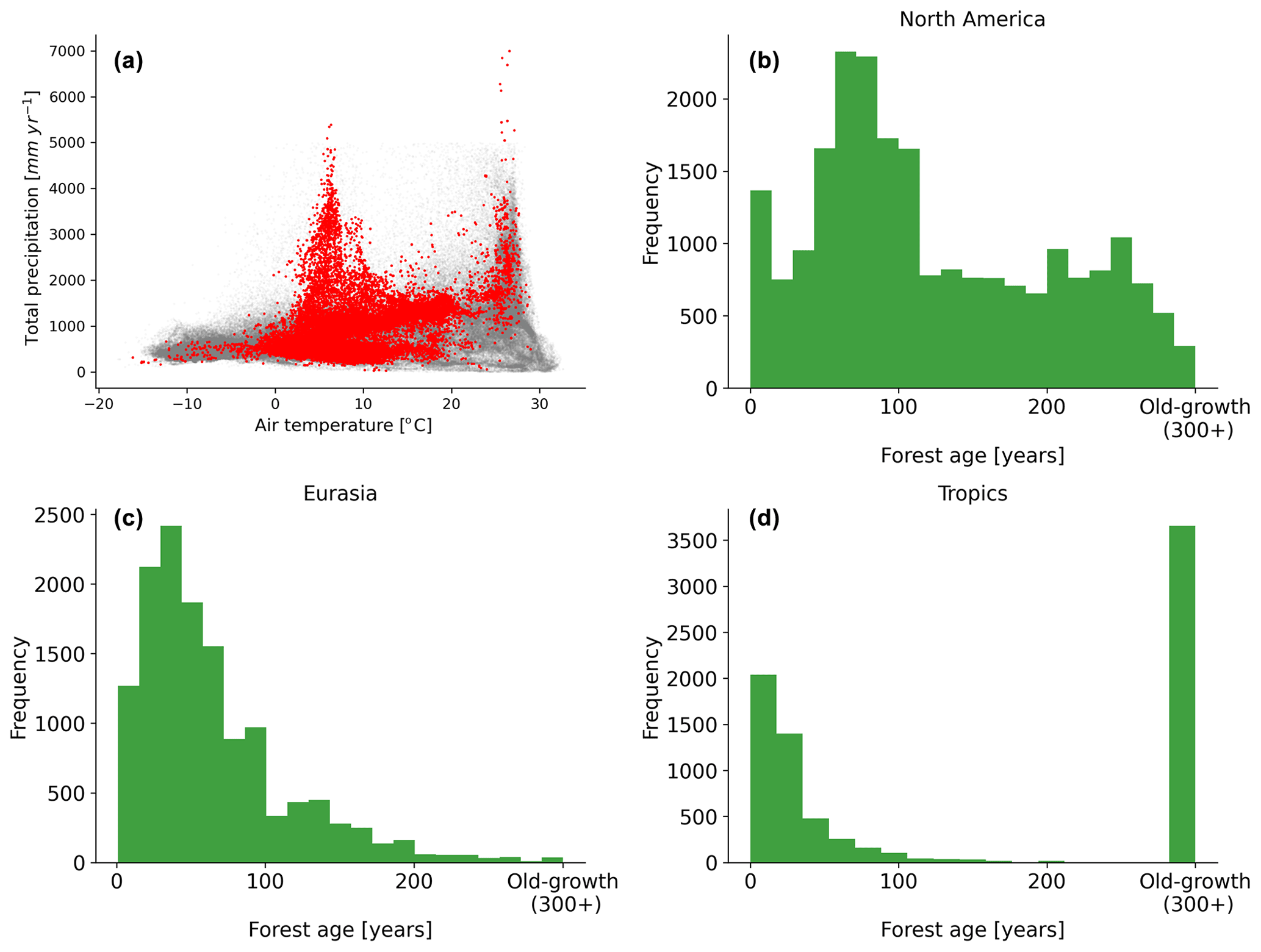
Figure 2 Distribution of the forest inventory plots in a climate space defined by air temperature and total annual precipitation (a). Histogram distributions of the forest age observations in North America (b), Eurasia (c) and the tropics (d) are also shown. The grey dots show the global distribution of a 0.25^∘ grid-cell forest in climate space defined by air temperature and precipitation, while the red dots show the distribution of the forest inventory data in the same climate space.

A comprehensive meta-analysis of the compiled dataset (Fig. 2) revealed that the observations covered a large spectrum in the climate space (Fig. 2a), although there were few plots in hot and dry regions, likely due to the low presence of forest ecosystems in such regions. We further described the age spectrum covered at the regional scale and found that a large spectrum of forest age was covered in North America (Fig. 2b) and Eurasia (Fig. 2c), while in the tropics, biases were observed (i.e. a significant fraction of tropical old-growth forests and relatively young forests) (Fig. 2d).

For each forest inventory plot, we extracted bioclimatic variables from WorldClim version 2 (Fick and Hijmans, 2017). In addition, we extracted all the soil-related variables of the Harmonized World Soil Database v 1.2 dataset. Finally, we derived a series of proxies for disturbance and management regimes from the Hansen tree cover dataset (Hansen et al., 2013).

• The intensity of tree loss from the Hansen tree cover loss layer: this metric was derived by counting the 30 m pixels that experienced a tree cover loss for 2000–2019 within a 1 km grid cell.

• Last time since tree cover loss from Hansen tree cover loss layer – standard deviation metric: this metric was calculated as the last time from 2019 since a 30 m pixel experienced tree cover loss, and we further computed the standard deviation of this last time since tree cover loss within a 1 km grid cell.

Table S1 in the Supplement summarizes the list of covariates considered in our study. Two datasets were further created. First, we created a dataset that contained the plots with reported stand age estimates ranging from 1 to 299 years (hereafter non-old-growth forests dataset). Second, we created a binary dataset reporting whether an observation had an age estimate of less than 300 years old or whether an observation had an age estimate of more than or equal to 300 years old or not reported but considered old-growth tropical forests (0 for non-old-growth forest and 1 for old-growth forest) (hereafter old-growth forests dataset).

2.2 Feature selection and model training

From the set of predictors related to vegetation and climatic conditions (Table S1), we performed a feature ranking with a recursive feature elimination (RFE) procedure (https://scikit-learn.org/stable/modules/generated/sklearn.feature_selection.RFE.html, last access: 22 October 2021) (Guyon et al., 2002) both on the non-old-growth forest and old-growth datasets. The 10 best covariates selected by the RFE algorithm were further used to train either a random forest (RF) regressor algorithm (RFregressor) (https://scikit-learn.org/stable/modules/generated/sklearn.ensemble.RandomForestRegressor.html, last access: 22 October 2021) or an RF classifier algorithm (RFclassifier (https://scikit-learn.org/stable/modules/generated/sklearn.ensemble.RandomForestClassifier.html, last access: 22 October 2021). As such, two distinct models were implemented. The RFregressor model was used to estimate forest age in the non-old-growth forests dataset, while the RFclassifier model was used to classify old-growth vs. non-old-growth forests using the old-growth forests dataset. The performances of the two models were assessed using leave-one-cluster-out cross-validation to reduce possible spatial auto-correlation between the training and test sets (Ploton et al., 2020). A cluster of plots contained all the plots within the same pair of latitude and longitude coordinates rounded to the nearest 10^∘ (e.g. latitude of 20^∘ and longitude of 110^∘) (see Fig. 1). For the RFregressor model, the root-mean-square error (RMSE), normalized root-mean-square error (NRMSE) and Nash–Sutcliffe model efficiency coefficient (NSE) were used for assessing the predictive capacity of the model for predicting forest age. For the RFclassifier model, we reported the precision (i.e. the number of correctly identified members of a class divided by all the times the model predicted that class), recall (i.e. the number of members of a class that the classifier identified correctly divided by the total number of members in that class) metrics and F1 score (i.e. the combination of precision and recall). Additionally, we explored functional relationships between the variables selected by the feature selection procedure and stand age in the RFregressor model by using the Tree Shapley Additive Explanations (TreeSHAP) algorithm (Lundberg and Lee, 2017; Lundberg et al., 2019). A negative SHAP value for a given variable X translates a negative contribution to the local changes in forest age and vice versa.

2.3 Upscaling procedure

To upscale the two trained models (i.e. RFclassifier and RFregressor models) from plot-level data to the global scale, we collected climate grids from the WorldClim dataset (Fick and Hijmans, 2017) and a series of agb grids circa 2010 (i.e. corrected for tree cover with thresholds of 0 %, 10 %, 20 % and 30 %) from the Globbiomass project (http://globbiomass.org/, last access: 22 October 2021) (Santoro et al., 2021). The tree cover correction was done by masking out the 100 m pixels in the original agb product (i.e. 100 m resolution) with tree cover estimates (Hansen et al., 2013) below one of the tree cover thresholds mentioned above within a 1 km extent. The original filtered agb maps were aggregated from 100 m to 1 km spatial resolution with a bilinear resampling method.

The upscaling procedure was done in two steps. First, each 1 km pixel was classified as old-growth or non-old-growth forests using the trained RFclassifier model. Second, the 1 km pixels classified as non-old growth were assigned with an age estimate ranging from 0–299 years inferred from the RFregressor model, while the pixels classified as old-growth forest were assigned a default age value of 300 years. In total, four gridded forest age maps with a 1 km spatial resolution were obtained using the different agb maps derived from the different tree cover thresholds as mentioned above (hereafter MPI-BGC – Max Planck Institute for Biogeochemistry – forest age datasets). We also created maps from the 1 km resolution forest age maps that reflected the fraction of several age classes (0–300+ with decadal resolution) within each 0.5^∘ grid-cell resolution.

3 Results and discussion

3.1 Model development and evaluation

We used the 10 most important variables from the set presented in Table S1 identified by the RFE algorithm procedure for the RFregressor and the RFclassifier models (Table 1). This set of selected variables was further used to train the two models in the cross-validation analysis and the global upscaling procedure.

Table 1 List of the predictors confirmed as important by the feature selection algorithm for RFregressor and the RFclassifier models. See Table S1 for details on the variable names.

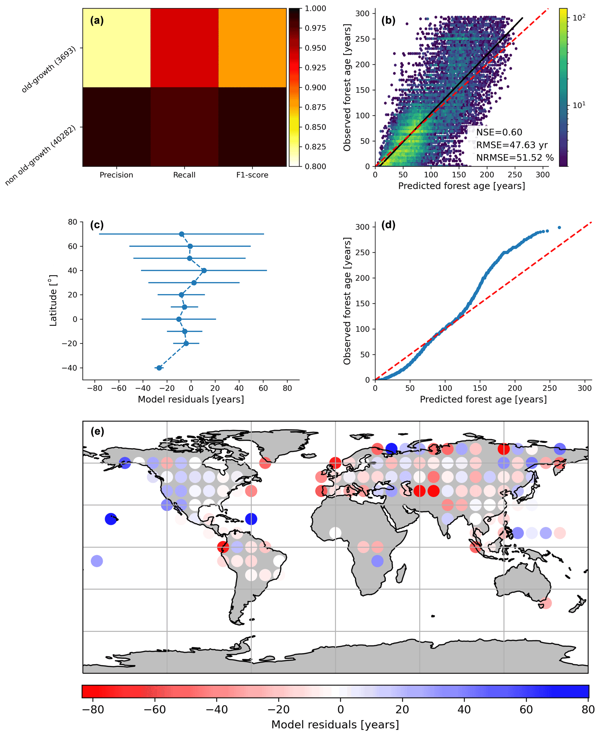
Figure 3 Cross-validated results of the old-forest vs. non-old-forest classification (a) and comparison of predicted vs. observed forest age estimates from the regression model (b). In (c), the average model residuals ∓ standard deviation within 10^∘ latitudinal beans is shown. The quantile–quantile plot (d) is also shown.

By assessing the cross-validation results, we found that the RFclassifier model could accurately partition old-growth and non-old-growth forests with precision estimates of 0.81 and 0.99 for old-growth and non-old-growth forests, respectively (Fig. 3a). Furthermore, we found recall values of 0.94 and 0.98 for old-growth and non-old-growth forests, respectively, while we found F1 scores of 0.87 and 0.99 for old-growth and non-old-growth forests, respectively (Fig. 3a). The performance of the RFregressor model was relatively high (NSE = 0.60, RMSE = 47.63 years and NRMSE = 51.52 %) (Fig. 3b), while the model residuals across 10^∘ latitudinal averages were relatively low (Fig. 3c). However, the quantile–quantile plot depicted biases in both very young and old forests (Fig. 3d). More precisely, the RFregressor model slightly overestimated the age estimates of young forests while underestimating the age estimates of older forests (i.e. > 150 years old) at the plot level. The biases for the very young or the older forests were possibly due to the properties of the training dataset in which older forests are still largely underrepresented compared to younger stands (Fig. 2a–c) (i.e. skewed distribution of the age estimates). Such biases could potentially be propagated from the plot level to the global scale and have implications in representing the location of younger and older forests globally. Figure 3e shows the spatial patterns of the model residuals. For instance, we observed that the RFregressor model underestimated the age estimates in most North American forests, while it overestimated the age estimates in most European forests.

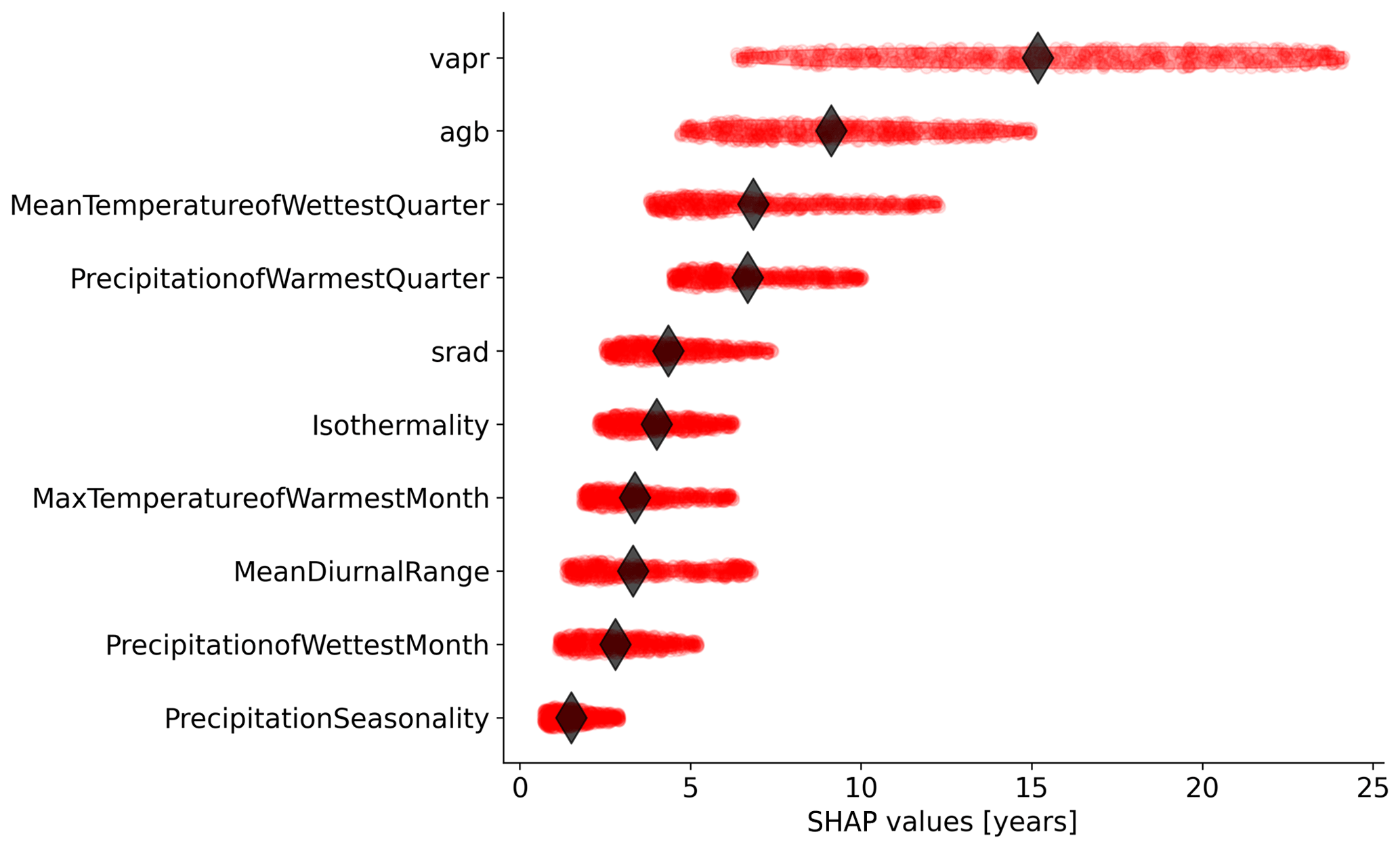
Figure 4 Relative importance of the independent variables selected by the feature selection algorithm in predicting forest age estimates in the RFregressor model. Each dot represents the absolute SHAP value of one observation. The diamond represents the median value for each variable.

We further investigated the variable importance of the selected variables and the functional relationships learned by the RFregressor model between forest age and these selected variables. For this, we computed the SHAP values for each predictor to show how each predictor contributes, either positively or negatively, to the forest age estimates. First of all, we observed that vapr was the most important variable, followed by agb and MeanTemperatureofWettestQuarter (Fig. 4). The importance of atmospheric-water demand in explaining stand age variability could indicate how biomass is associated with stand age across different climate regimes. More precisely, such observations could imply that high atmospheric-water demand limits growth rates and maximum biomass, thereby indirectly controlling how biomass relates to age. In addition, high atmospheric-water demand might influence fire frequency (Mueller et al., 2020) and indirectly control forest age distribution through the effect of fire on biomass. Biomass estimates contain information about the current state of the forest, integrating the cumulative effect of land use change, management and disturbance history. Therefore, having biomass (i.e. agb) as an important variable in predicting forest age confirmed strong management and disturbance regime controls on the forest age distribution (Amiro et al., 2010).

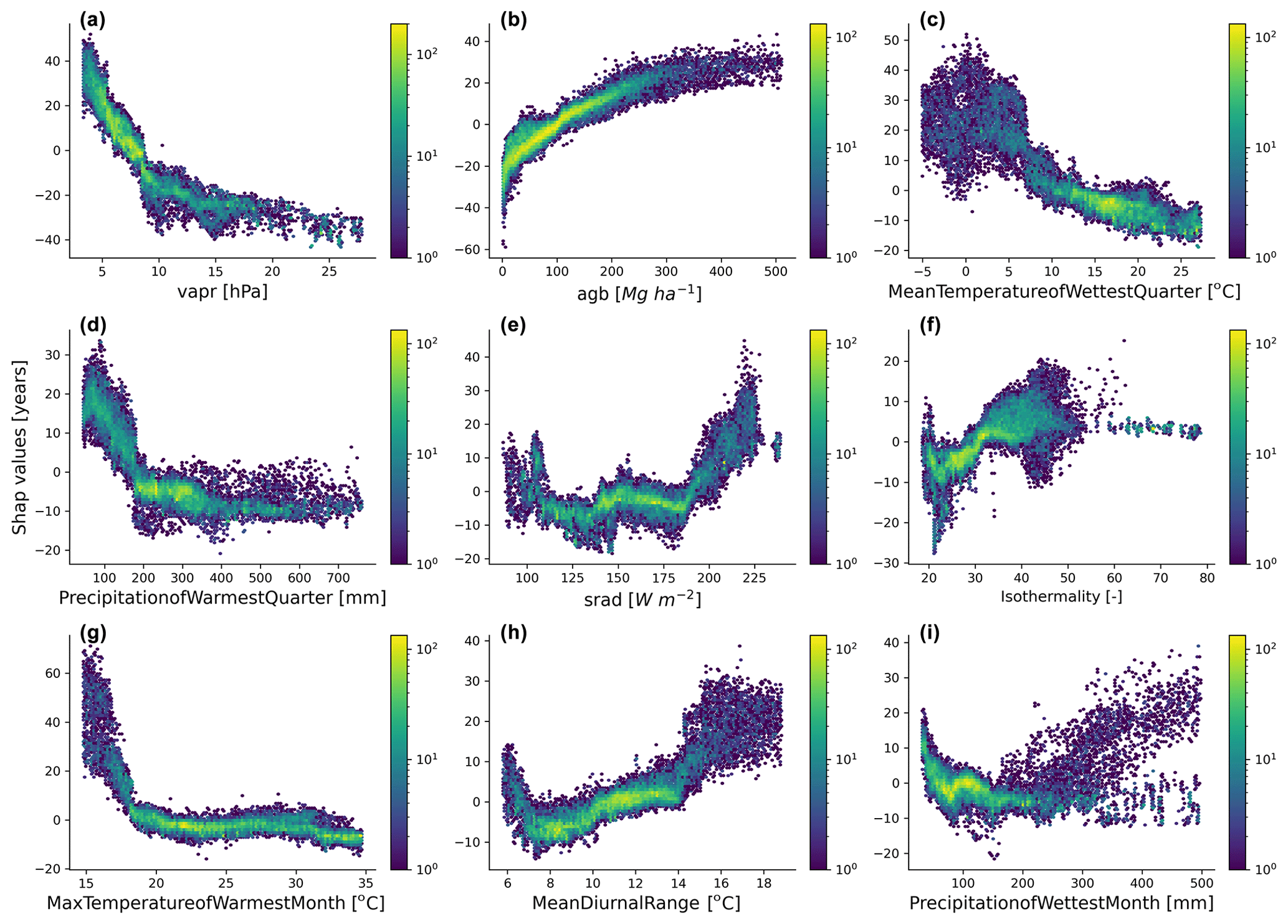
Figure 5 Emergent relationships between the retrieved SHAP values and the independent variables selected by the feature selection algorithm.

The emergent relationships revealed that an increase in agb was associated with an increase in the forest age estimates (Fig. 5b). This relationship was expected as older trees have more carbon stored in their aboveground components than younger forests. The modelled forest age estimates appeared to be also relatively sensitive to the climatic conditions. For instance, we observed that climatic conditions with low atmospheric-water demand (i.e. low vapr) (Fig. 5a) or conditions with high solar radiation (Fig. 5e) increased forest age. Similarly, we observed that forest age variability was also associated with air temperature conditions (Fig. 5c, f, g and h) and precipitation regimes (Fig. 5d and i).

3.2 Global forest age patterns and regional overview

The MPI-BGC forest age product shows an extensive range of forest age across the globe (Fig. 6). We observed that the most represented age class was the old-growth forests with around 1.3 billion hectares, while a limited fraction of very young forests was observed (i.e. < 10 years old) (Fig. 6a). Not surprisingly, most of the old-growth/undisturbed forests (>300 years old) can be found in the Amazon basin (Fig. 6b), the Congo basin (Fig. 6c) and part of the Indonesian peninsula (Fig. 6h), where minimal human disturbance occurred. A large area occupied by very young forests was found in the southeastern part of China (Fig. 6h), probably due to afforestation/reforestation policies and natural disturbances (Zhang et al., 2017). Similarly, young and intermediate forests were found in African tropical dry forests (i.e. Sahel and Miombo regions) (Fig. 6c), where the frequency of fire regimes is very high, resulting in a relatively young age-class structure (Werf et al., 2017). Large-scale fires in the North American boreal region also resulted in widespread patches of younger forests and a mosaic of stands of different ages since they last burned (Fig. 6g).

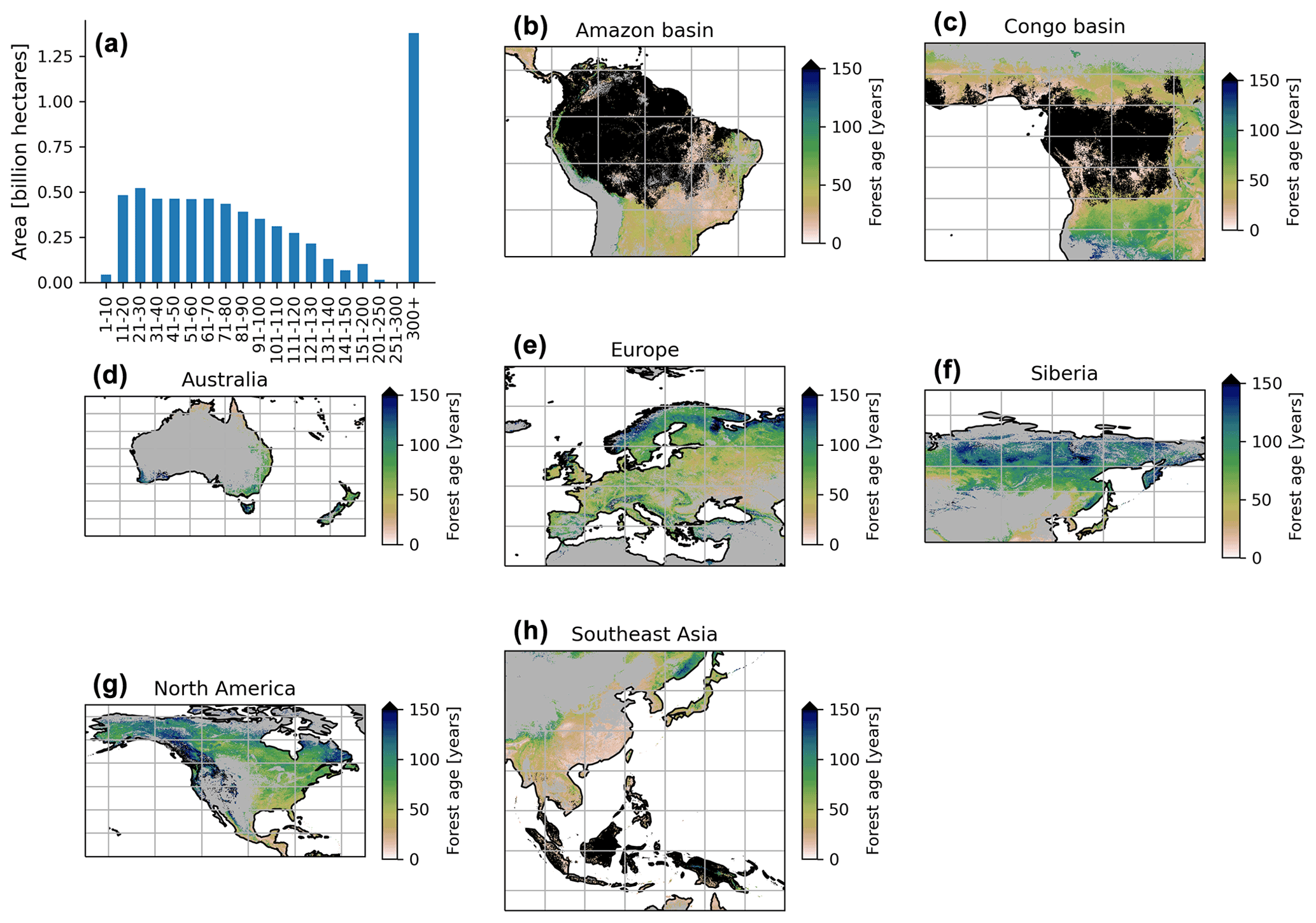
Figure 6 Total area of each age class globally (a) and close-up examples in the Amazon basin (b), Congo basin (c), Australia (d), Europe (e), Siberia (f), North America (g) and Southeast Asia (h). The forest age estimates in the close-up examples (b–h) range from 0 to 150 years old for a better visualization. The forest age map using a 10 % tree cover threshold is shown.

Furthermore, the unmanaged part of the North American boreal region near the ecotone, where fires are infrequent, revealed older stands (Fig. 6g). Forests in British Columbia were generally old, although patches of younger forests were probably in the early stages of disturbance recovery. European forests were in young/intermediate stages of forest succession (Fig. 6e). The increased harvested forest area and considerable afforestation practices (Naudts et al., 2016) probably explained a relatively young- to intermediate-forest demography and a mosaic of different age classes in the European region. The region of Siberia revealed a gradient of younger to older forests going from the southern to the northern part of the Siberian region (Fig. 6f). Such an observation could suggest different fire regimes between southern and northern Siberia and confirm harvesting practices identified in southern Siberia (Curtis et al., 2018). Finally, Australian forests were relatively young in the northern part of the country, while a mosaic of age classes dominated the southern part of Australia (Fig. 6d). The age patterns observed in the northern part of Australia somehow correspond to the fact that forests are regrowing in this region (Pugh et al., 2019). However, it is essential to note that the few forest inventory plots in regions such as Australia (Fig. 1) could limit our certainty on the forest age estimates attributed by the statistical approaches due to, for instance, extrapolation issues. Another limitation is that we assumed forest homogeneity within a 1 km grid cell, which would reduce the extremes of low and high biomass estimates in the gridded global products that the models have learned in the plot-level training data. This limitation might, for instance, explain the relative dearth of very young stands (1–10 years old) in the MPI-BGC global age product (Fig. 6a).

3.3 Global forest age relationships with the atmosphere, hydrosphere and vegetation conditions

We further investigated the distribution of the forest demography in the climate and vegetation spaces (Fig. 7). Generally, we observed that with warmer (i.e. air temperature) and drier (i.e. VPD – vapour pressure deficit) conditions, forests appeared to be younger with the expectation of old-growth tropical forests located in relatively warm climatic conditions (Fig. 7a). Not surprisingly, we found that most of the old-growth tropical forests were located in regions with high productivity (i.e. high GPP – gross primary production – and high biomass) (Fig. 7b), which coincides with our previous results investigating the structure of the statistical model showing that an increase in forest biomass was coupled with an increase in forest age (Fig. 5a). On the other hand, we observed that younger–intermediate forests were more productive than older forests outside the tropical old-growth forest envelope. More precisely, we found that forests being less productive will belong to an older age class for similar carbon stocks. Mature forests were found in cool temperatures and moderately low-precipitation conditions (Fig. 7c), where rates of fast growth but slow decomposition generally drive forest dynamics. Younger stands were found in relatively warm conditions but a wide range of precipitation regimes (Fig. 7c). Finally, while a significant fraction of young forests were located in regions with low water availability and high atmospheric-water demands, we also observed that above a certain threshold of water availability (i.e. > 0.4–0.5), the amount of water available for trees (i.e. IWA – index of water availability) was not directly associated with changes in forest age unlike VPD (Fig. 7d).

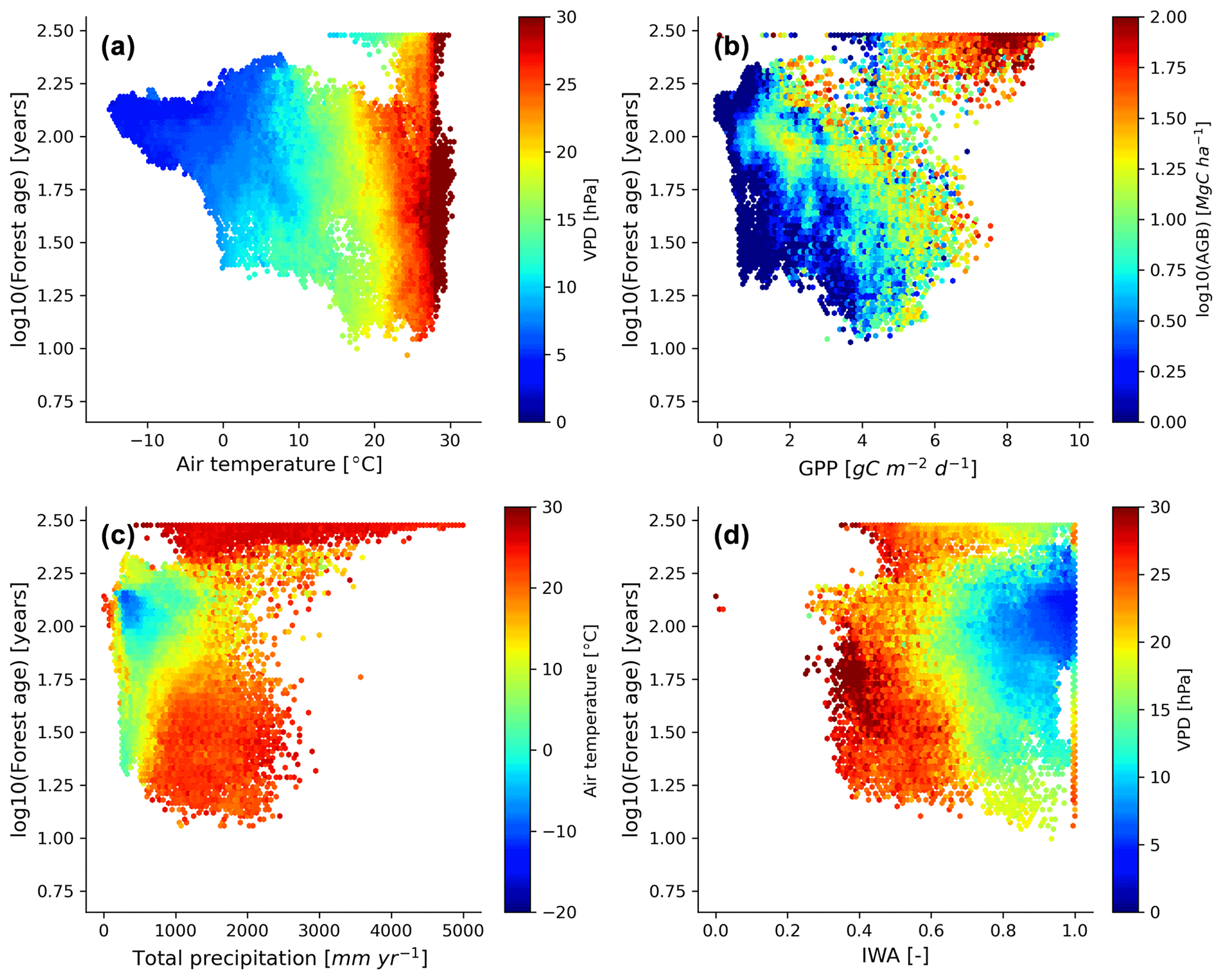
Figure 7 Forest age distribution with the climate and hydrological and productivity spaces defined by air temperature, vapour pressure deficit, total precipitation, soil water availability, GPP and aboveground biomass. The forest age map used here corresponds to a tree cover threshold of 10 % aggregated to 0.25^∘ using a weighted average of all non-NODATA contributing pixels. GPP is gross primary productivity derived from the FLUXCOM RS+meteo (remote sensing) product (Tramontana et al., 2016; Jung et al., 2011, 2020), and IWA is an index for soil water availability (Tramontana et al., 2016). The climatic variables were retrieved from the ERA5 reanalysis data (https://apps.ecmwf.int/datasets/licences/copernicus/, last access: 22 October 2021). For all the climatic variables, we computed an annual mean for the year 2010.

3.4 Sensitivity analysis, uncertainties and comparison with previous products

We performed a sensitivity analysis using a series of agb gridded products filtered with different tree cover thresholds to produce different global age products (see “Method”) (Fig. 8). This analysis showed that in South America, mainly the dry regions were sensitive to the tree cover threshold being applied, with forest age estimates being lower when no tree cover threshold was applied compared to a 30 % tree cover correction (Fig. 8a). Similarly, we observed that the dry parts of the Congo basin depicted a sensitivity to the applied tree cover thresholds (Fig. 8b). In Europe, we observed widespread differences between the forest age estimated without a tree cover correction and with a tree cover correction (Fig. 8c). Generally, forest age estimates were higher when the 30 % tree cover correction was applied. In Siberia (Fig. 8d), North America (Fig. 8e) and Southeast Asia (Fig. 8f), there were also large patches of forest where correcting the biomass maps with a tree cover threshold led to substantial differences in the age estimates. Overall, such observations were expected because of management practices or disturbance regimes, resulting in mosaic vegetation within a 1 km grid cell. Such mosaic vegetation in regions such as the dry tropics (forest, grassland or shrubland), Europe (forests or croplands) and the northeast of the United States (forests or croplands) could explain the sensitivity of the forest age estimates to tree cover thresholds in these regions.

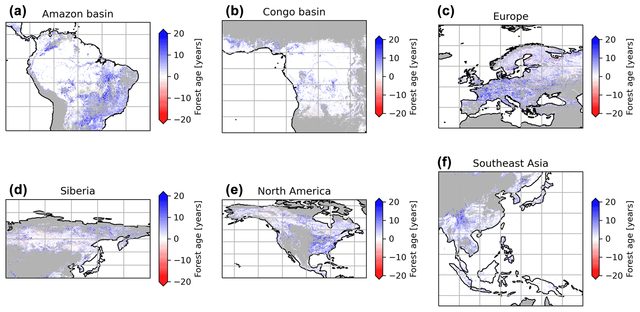
Figure 8 Sensitivity of the presented age product using 30 % tree cover correction thresholds or no tree cover correction. The differences between the age estimates derived from a forest biomass product using a 30 % tree cover correction and the age estimates derived from a forest biomass product not using a tree cover correction are shown. The blue colour means that the age estimates are higher with the 30 % tree cover correction than without correction, while the red colour means that the age estimates are lower with the 30 % tree cover correction than without correction.

Besides, we explored uncertainties associated with the two statistical models used for the upscaling procedure (Figs. S1–S3 in the Supplement). First, we observed that the RFclassifier model had very high probabilities of classifying either a non-old-growth or an old-growth forest at the pixel level, as the fraction of the random forest ensemble to classify the two forest classes was generally close to 1 (Figs. S1 and S2), suggesting relatively high confidence in the partitioning between old-growth and non-old-growth forests in the MPI-BGC forest age product. The regions at the edge of the Amazon and the Congo basins appeared to have the lowest confidence in classifying old-growth vs. non-old-growth forests (Figs. S1a and b and S2) with a probability close to 0.5. On the other hand, we observed relatively high probabilities for classifying non-old-growth forests in Europe (Fig. S1c), Siberia (Fig. S1d), North America (Fig. S1e) and Southeast Asia (Fig. S1f). We also provided uncertainties in predicting forest age estimates by retrieving the 25 %, 50 % and 75 % quantile predictions from the RFregressor model for computing the inter-quantile range (IQR; quantile 75 % – quantile 25 %) divided by the median (i.e. quantile 50 %) of the forest age estimates (IQR and median) (Fig. S3). While in Europe (Fig. S3c), China (Fig. S3f) and the eastern United States (Fig. S3e), the IQR and median estimates were relatively low, we observed high IQR and median estimates in northern North American regions (Fig. S3e) as well as in large patches of Siberia (Fig. S3d) and the dry tropics (Fig. S3a and f).

Figure 9 Comparison between the forest age dataset from this study and an independent forest age dataset: Amazon basin (a and b), China (c and d) and North America (e and f). For a fair comparison with the independent age datasets, the MPI-BGC forest age map used here is the one without tree cover correction applied to the agb dataset. Differences were computed using weighted age estimates from the fraction of the decadal age classes within each 0.5^∘ grid-cell resolution.

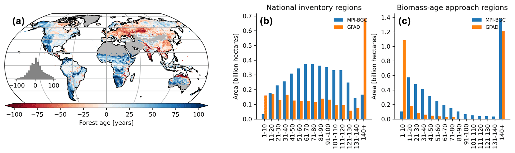
Figure 10 Difference map between the forest age estimates derived from the MPI-BGC and GFAD products (a). Areas per age class were also compared between the two products for regions relying on national inventories (b) and relying on the biomass–age approach (c) in the GFAD product. Differences were computed using weighted age estimates from the fraction of the decadal age classes within each 0.5^∘ grid-cell resolution.

We further compared the spatial patterns of the MPI-BGC forest age dataset with a series of independent regional and global forest age products (Chazdon et al., 2016; Pan et al., 2011; Poulter et al., 2019; Zhang et al., 2017) (Figs. 9 and 10 and S5 in the Supplement). In the Amazon basin, we found that the MPI-BGC forest age product depicted widespread higher forest age estimates (i.e. blue colour) than the Chazdon et al. (2016) dataset (Fig. 9a), resulting in a more extensive area of tropical old-growth forests in the MPI-BGC forest age product (Fig. 9b). On the other hand, we observed lower forest age estimates in the regions of Rio Grande do Norte and Paraíba in the MPI-BGC forest age product (i.e. red colour). Such disagreement between the two products could be related not only to the different methods used to infer forest age (i.e. statistical method vs. age–agb chronosequence approach for the MPI-BGC forest age and the Chazdon products, respectively) but also to the uncertainties of the RFclassifier for classifying old-growth vs. non-old-growth forests in this region (Figs. S1 and S2). Similarly, the presented product and the Pan dataset revealed widespread discrepancies in the North American region, particularly in the western part of the United States and the North American boreal forests (Fig. 8e). More precisely, the Pan dataset had a higher fraction of young-forest patches than the MPI-BGC forest age product (Fig. 9f). Methodological differences between the Pan and the MPI-BGC forest age datasets could explain such differences. While the Pan dataset integrates forest inventories, disturbance datasets, and land use and land cover change data to retrieve forest age estimates, the MPI-BGC forest age product relied on forest inventory, climate data and statistical methods. Additionally, forest inventory plots used to derive the MPI-BGC forest age product were relatively sparse in Canada (Fig. 1), which might limit the statistical methods used for the MPI-BGC forest age product to predict realistic forest age estimates (i.e. extrapolation issues). Finally, the forest age estimates of China's MPI-BGC forest age product were consistent with the Zhang dataset (Fig. 9c). The area distribution across age classes of the two products appeared to have a relatively good agreement in China (Fig. 9d).

We also found significant and widespread discrepancies between the MPI-BGC forest age dataset and the global forest age dataset (GFAD) (Poulter et al., 2019) (Fig. 10). Overall, the GFAD product had higher fractions of very young and old forests (Fig. 10b and c). Because the GFAD used a different agb product for the pan-tropical region and mainly relied on statistics from national forest inventories for the Northern Hemisphere, widespread differences were expected between the GFAD and the MPI-BGC forest age maps. The MPI-BGC forest age dataset depicted older forests in the western part of the United States (i.e. blue colour), while it showed younger forests across Europe than the GFAD product (Fig. 10a). Differences were also apparent in the dry tropics, where the GFAD product showed younger forests than the MPI-BGC forest age dataset, particularly in the Miombo region. Such discrepancies could be explained either by the use of a biomass–age approach in this region or by integrating MODIS (Moderate Resolution Imaging Spectroradiometer) fire information in the GFAD forest age dataset. We adjusted the MPI-BGC forest age dataset with the forest age product inferred from the MCD45A1 MODIS fire product at 1 km resolution (Giglio et al., 2018; Poulter et al., 2019), which was used in the GFAD product. In this MODIS–age product, forest age was determined as the last time since a fire event occurred within a grid cell for 2000–2015, thereby assuming that the entire pixel was burned down. For instance, forest age within a 1 km grid cell was 5 years old if the last time a fire occurred within this grid cell was in 2010. The latter took precedence over the former dataset when adjusting the MPI-BGC forest age dataset with the MODIS–age product. As expected, we observed a higher fraction of younger forests in the adjusted MPI-BGC forest age dataset (Fig. S4b in the Supplement), particularly in regions relying on the biomass–age approach in the GFAD product (Fig. S4a and c). However, significant discrepancies between the two products remained when comparing the weighted average forest age estimates at the pixel level, particularly in European forests (Fig. S4a). Yet, we acknowledge that a comparison between the GFAD and the MPI-BGC forest age maps has to be taken with caution when evaluating the MPI-BGC product, as substantial methodological differences exist between the two products.

4 Data availability

The dataset of the different forest age products presented in this study can be downloaded from the Data Portal of the Max Planck Institute for Biogeochemistry at https://doi.org/10.17871/ForestAgeBGI.2021 (Besnard et al., 2021).

5 Conclusions

We presented a new forest age dataset derived from forest inventory, biomass, climate and remote sensing data. Generally, the statistical model used to create the gridded age datasets had a relatively good capacity to predict forest age estimates at the plot level (precision of 0.81 and 0.99 for classifying old-growth and non-old-growth forests, respectively, and NSE of 0.6 for predicting non-old-growth forests). At the same time, biases were observed, mainly when predicting older forests (i.e. > 150 years old). The functional relationships between biomass and forest age learned by the statistical models appeared to agree with forest age theory and the role of the environment and climate in modulating the relationship. The proposed gridded datasets allowed us to assess the global patterns of forest age and provided insights into regional forest demography. For instance, relatively young–intermediate forests were observed in Europe and China, areas with predominant management practices and afforestation/reforestation activities. We could also demonstrate that old forests are primarily represented in very wet, warm and cold regions. However, comparing the MPI-BGC forest age product with independent forest age datasets revealed large discrepancies, suggesting high uncertainties in mapping forest demography globally. Overall, this forest age product provides a new source of information related to disturbance history and forest regrowth, which is crucial to better understanding the location of the forest carbon sinks and sources.