A detailed radiostratigraphic data set for the central East Antarctic Plateau spanning from the Holocene to the mid-Pleistocene

We present an ice-penetrating radar data set which consists of 26 internal reflecting horizons (IRHs) that cover the entire Dome C area of the East Antarctic plateau, the most extensive to date in the region. This data set uses radar surveys collected over the space of 10 years, starting with an airborne international collaboration in 2008 to explore the region, up to the detailed ground-based surveys in support of the Beyond EPICA – Oldest Ice (BE-OI) European Consortium. Through direct correlation with the EPICA-DC ice core, we date 19 IRHs that span the past four glacial cycles, from 10 ka, beginning of the Holocene, to over 350 ka, ranging from 10 % to 83 % of the ice thickness at the EPICA-DC ice core site. We indirectly date and provide stratigraphic information for seven older IRHs using a 1D ice flow inverse model, going back to an estimated 700 ka. Depth and age uncertainties are quantified for all IRHs and provided as part of the data set. The IRH data set presented in this study is available at the US Antarctic Program Data Center (USAP-DC) (https://doi.org/10.15784/601411, Cavitte et al., 2020) and represents a contribution to the SCAR AntArchitecture action group (AntArchitecture, 2017).

1 Introduction

Extensive ice-penetrating radar data have been collected over the years in the Dome C region of the East Antarctic Plateau. These data were initially collected to characterize the Dome C ice core site. Subsequently, the Dome C region was revealed as one of the promising regions to have retained million-year-old ice, based on modeling thermodynamic results (Van Liefferinge and Pattyn, 2013; Fischer et al., 2013; Van Liefferinge et al., 2018). The rare combination of thick ice, relatively low snow accumulation rate, low geothermal heat flux, slow ice flow and clear undisturbed englacial stratigraphy made this site one of the primary target drilling sites for the Beyond EPICA – Oldest Ice European project (BE-OI), with the added advantage of its proximity to the Concordia Station for logistics (Fig. 1). Providing detailed constraints on the ice sheet in this region including its internal age structure and its temporal flow stability motivated the extensive tracing of internal stratigraphy over the entire Dome C region. All published radar data sets available in this region were used to construct the internal stratigraphy presented here.

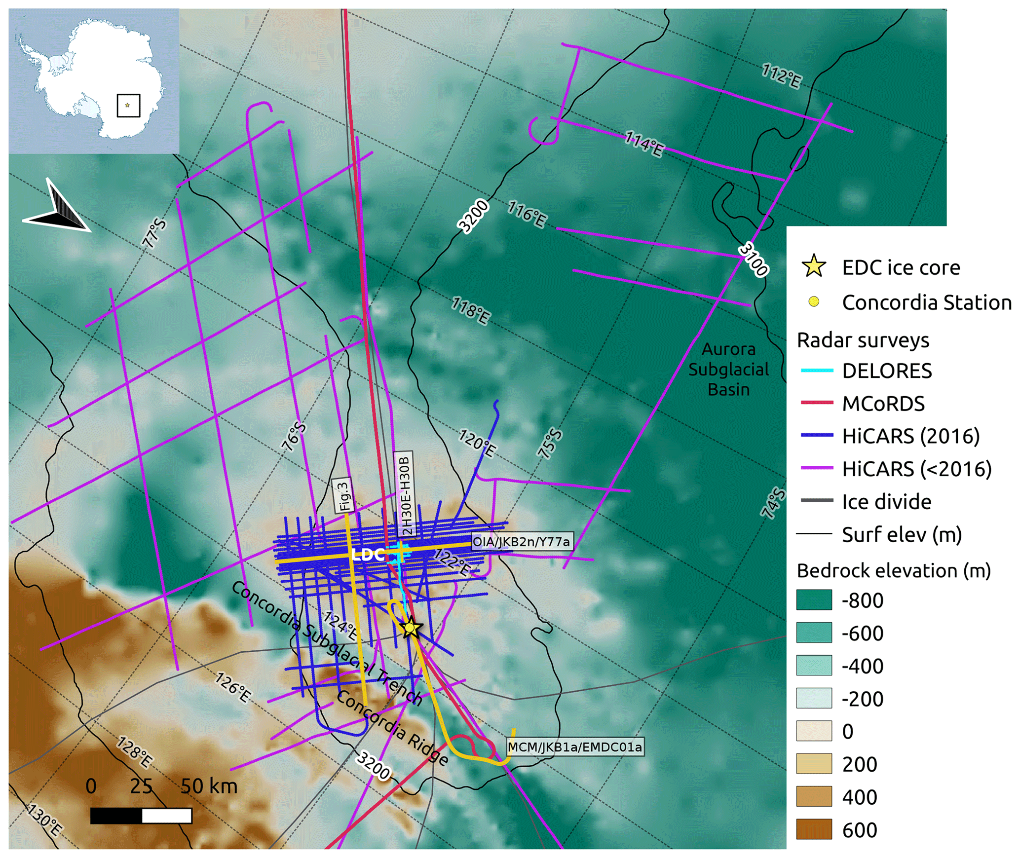
Figure 1 The Dome C region of the East Antarctic plateau with the extent of the ice-penetrating radar surveys used to trace the IRHs, shown as solid lines whose color is shown in the legend. Radar transects discussed are highlighted in yellow. Background is BedMachine Antarctica v1 bedrock topography (Morlighem et al., 2020) with superimposed CryoSat-2 elevation contours (Helm et al., 2014); a yellow star and a yellow circle locate the EDC ice core site and the Concordia Station, respectively (note that they are coincident at this spatial scale); a gray line locates the Rignot et al. (2019) ice divides in the region; the main geographical sites are labeled. The inset locates the study area. This figure was prepared with Quantarctica (Matsuoka et al., 2021).

Ice-penetrating radar became the prime method to image the hidden bedrock beneath the ice and derive ice thickness in the 1960s (Robin et al., 1969). By the 1970s, the internal stratigraphy of the ice column started being examined including the origin of the internal reflecting horizons (IRHs) (Clough, 1977). IRHs can have three possible origins: (1) density changes, typically restricted to the firn column; (2) ice chemical composition variation, and therefore conductivity variation, resulting from the successive deposition and burial of aerosols and dust particles on the ice; and/or (3) ice fabrics (Clough, 1977; Millar, 1981; Fujita and Mae, 1994; Siegert et al., 1998b; Fujita et al., 1999), usually most strongly observed at depth or in areas of shear flow. The IRHs presented in this data set are thought to be dominated by conductivity variations, considering their relative depths and the relative flow stability of this part of the ice sheet. Such IRHs are generally assumed to be isochronous (Whillans, 1976; Siegert et al., 1998a) and, as a result, can be used as time markers and thus provide a dated stratigraphy as long as they are laterally continuous (Siegert, 1999; Fujita et al., 1999). Ages are generally assigned to the IRHs where the radar transects pass close to an ice core site, sometimes requiring some assumptions about how to interpolate between the point of closest approach and the ice core site (Siegert et al., 1998a; Winter et al., 2015; Cavitte et al., 2016; Bodart et al., 2021). IRHs have also been used extensively to characterize past and present flow conditions (Jacobel et al., 1993; Siegert et al., 2004; NEEM community members, 2013; Karlsson et al., 2014; Bingham et al., 2015; Kingslake et al., 2016; Beem et al., 2018), provide constraints in the reconstruction of past accumulation rates (Eisen et al., 2008; Casey et al., 2014; Koutnik et al., 2016), estimate englacial temperature (Matsuoka, 2011; MacGregor et al., 2012), and measure basal reflectivity and thus reveal subglacial hydrological drainage (Carter et al., 2007, 2009; Schroeder et al., 2015; Siegert et al., 2016) (see Schroeder et al., 2020, for more applications).

An extensive internal stratigraphic data set has already been obtained for the Greenland Ice Sheet (MacGregor et al., 2015). However, due to its sheer size and much lesser accessibility, but also the wide variety of data acquisition platforms and processing algorithms applied to the data as a result of the multitude of institutes involved in data collection, the Antarctic Ice Sheet will require more time and the acquisition of additional ice-penetrating radar data in order to (1) connect existing surveys and (2) extend coverage to under-surveyed parts of the ice sheet. The SCAR action group AntArchitecture was commissioned for this specific purpose (AntArchitecture, 2017). The construction of a comprehensive Antarctic-wide IRH data set will both play a key role for projects such as the Beyond EPICA – Oldest Ice European search for million-year-old ice (Van Liefferinge and Pattyn, 2013; Parrenin et al., 2017) and provide valuable additional constraints for inverse models, potentially helping in cases where a unique solution could not be found due to a lack of data constraints (a persistent problem until now, e.g., Morse et al., 1998; Eisen et al., 2008; Koutnik et al., 2016; Parrenin et al., 2017; Muldoon, 2018) or providing large-scale constraints to 1D, 2D and 3D ice flow models (e.g., Leysinger Vieli et al., 2007, 2011; Passalacqua et al., 2018; Muldoon, 2018; Sutter et al., 2021).

Here we provide a spatially extensive IRH data set (data set release: Cavitte et al., 2020, https://doi.org/10.15784/601411), centered on the Dome C region of the central East Antarctic Plateau. The ages of the IRHs are established using the AICC2012 ice core chronology (Bazin et al., 2013; Veres et al., 2013). The radar transects were collected over a period of 10 years, by several institutes and under numerous projects. We archive this data set based on the standards established by previous IRH data contributions (e.g Winter et al., 2019; Bodart et al., 2021; Beem et al., 2021), adapted to fit the information available for this specific data set.

2 The Dome C Plateau region

The Dome C region is a topographic high (∼3233 m a.s.l.) in the interior of the East Antarctic Plateau at the intersection of multiple ice divides (Fig. 1), and in particular the ice divide separating the Byrd Glacier and the Totten Glacier catchments. The ice surface topography is gentle with a change in elevation of ∼10 m every 50 km (Genthon et al., 2016). A saddle connects Dome C to Lake Vostok farther south along the ice divide. A secondary dome is present ∼30 km south of Dome C, referred to as Little Dome C (LDC). The ice flow speed in the region is very low, a few mm yr⁻¹ at Dome C, up to ∼0.21 m yr⁻¹ 25 km from the summit (Vittuari et al., 2004). Surface temperatures are very low, reaching $\sim -\mathrm{54.5}$ ^∘C on average year-round (EPICA commmunity members, 2004). The bedrock topography in the Dome C region on the other hand is quite rough. A large subglacial massif is located just a few kilometers south of LDC, where the radar lines are the densest in Fig. 1, and bounded to the northeast by the deep Concordia Subglacial Trench and to the southwest by the Aurora Subglacial Basin (Young et al., 2017). The Concordia Subglacial Trench is itself bounded to the northeast by a 2000 m cliff, the Concordia Ridge. The LDC area was first highlighted as a key Beyond EPICA – Oldest Ice target site in the Van Liefferinge and Pattyn (2013) study. The ice core drilling site has since then been narrowed down to a precise location on LDC through successive radar survey collections (Young et al., 2017; Lilien et al., 2021) and modeling efforts (Parrenin et al., 2017; Cavitte et al., 2018; Van Liefferinge et al., 2018; Passalacqua et al., 2018), in preparation for drilling (Fig. 1).

3 Data and methods

3.1 Ice-penetrating radar systems

The IRHs were traced across multiple ice-penetrating radar surveys that deployed several generations of modern ice-penetrating radar sounders over a decade, between 2008 and 2018, over the Dome C region (Fig. 1). The primary set was collected by the University of Texas at Austin Institute for Geophysics (UTIG) and the Australian Antarctic Division (AAD) as part of the ICECAP project (International Collaborative Exploration of the Cryosphere through Airborne Profiling, Cavitte et al., 2016) between 2008 and 2015. This included the Oldest Ice candidate A (OIA) survey flown by ICECAP in January 2016 (Young et al., 2017). Data were collected with the High Capability Airborne Radar Sounder (HiCARS) 1 and 2 and its Multifrequency Airborne Radar-sounder for Full-phase Assessment (MARFA) descendant; in this paper we refer to these data as HiCARS. The ski-equipped DC-3T Basler was able to operate from Concordia Station, allowing for significant local coverage. The Vostok-Dome C airborne radar transect was flown by the Center for Remote Sensing of Ice Sheets (CReSIS) at the University of Kansas using the Multi-Channel Coherent Radar Depth Sounder (MCoRDS, version 2) in a single flight line in 2013. A P-3 Orion operating from McMurdo Station collected these data as part of NASA Operation Ice Bridge. We also use a subset of the LDC ground-based radar survey, towed behind a PistenBully PB300 tractor, collected by the Beyond EPICA – Oldest Ice (BE-OI) European Consortium using the British Antarctic Survey’s (BAS) Deep Looking Radio Echo Sounder (DELORES) radar system (King et al., 2009).

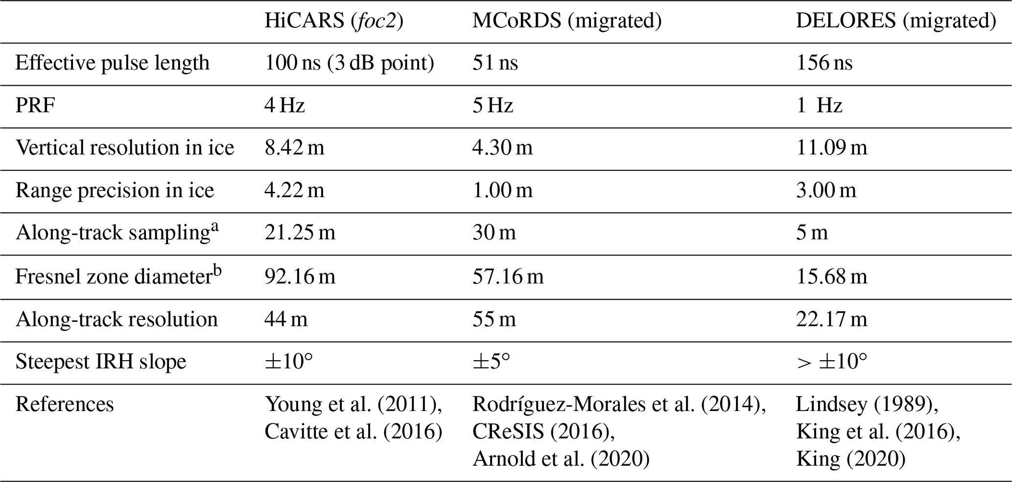
Peters et al. (2005)Arnold et al. (2020)Rodríguez-Morales et al. (2014)CReSIS (2016)King (2020)

Table 1 Ice-penetrating radar system characteristics before focusing and migration.

^* Holschuh et al. (2014).

Young et al. (2011)Rodríguez-Morales et al. (2014)Lindsey (1989)Cavitte et al. (2016)CReSIS (2016)King et al. (2016)Arnold et al. (2020)King (2020)

Table 2 Ice-penetrating radar post-processed data characteristics. Range precision is provided for an IRH with 6 dB SNR; Fresnel zone diameter and along-track resolution (after focusing and multilooking) are calculated at 1000 m depth in ice and an altitude of 500 m above the ice in the case of HiCARS and MCoRDS.

^a Of the final data product.
^b For a chirped system, the Fresnel zone diameter is calculated according to Haynes (2020, Eq. S.153):

$$\begin{array}{}\text{(1)}& F_{\mathrm{s}}=\mathrm{2}\sqrt{{\displaystyle \frac{C_{\mathrm{air}}}{\mathrm{2}{f}_{\mathrm{c}}}}(h+{\displaystyle \frac{z}{n}})}.\end{array}$$

For a signed waveform system, the Fresnel zone diameter is calculated according to Lindsey (1989):

$$\begin{array}{}\text{(2)}& F_{\mathrm{s}}={\displaystyle \frac{C_{\mathrm{ice}}}{\mathrm{2}{f}_{\mathrm{c}}\sqrt{\mathrm{2}{\mathit{ϵ}}^{\prime }}}}.\end{array}$$

Note that C_air is the electromagnetic velocity in air (3×10⁸ m s⁻¹), f_c is the center frequency of the radar system, h is the height of the aircraft above the ice, z is the depth of interest, TWTT is the two-way travel time to the depth of interest, n is the index of refraction of ice (1.78), and ϵ^′ is the relative dielectric permittivity of ice (3.17).

The main characteristics of each radar system are listed in Tables 1 and 2. The two fast-moving airborne systems improve the signal-to-noise ratio (SNR) of returning echoes by using long frequency-swept chirp waveforms that are pulse-compressed to narrow pulses. Of these two systems, HiCARS has the lowest frequency (60 MHz) and largest compressed-pulse width (100 ns; see Table 1). HiCARS' comparatively low frequency limits surface scattering losses but limits the along-track resolution that can be obtained after post-processing. For comparison, the MCoRDS radar system uses a center frequency between 180–210 MHz and a compressed-pulse width of 51 ns (Table 1).

The ground-based DELORES system uses a broadband impulse and improves SNR by moving slowly along the survey with a high pulse repetition frequency. Scattering losses are avoided by directly coupling the antenna to the surface. The ground-based nature of the survey allowed for very tight line spacing to be achieved; however, the area of coverage was limited compared to the airborne surveys.

3.2 Data processing

Data processing must be considered from the perspective of the radar system used and the properties of the targets to be imaged. A key tool is the use of synthetic aperture radar (SAR), which coherently combines echoes over an extended along track distance (the “aperture”) to correctly image sloping interfaces and cancel out scattered energy. Processing algorithms for ice are often optimized for the bed, which tends to be rough and scatter diffusively.

The IRHs tend to be distributed specular targets, which means that approaches designed to image the scattering bed are not necessarily appropriate for specular IRHs. In particular, the detected energy from a specular target will be limited to the coherent Fresnel zone, while the range of observable IRH slopes will be a function of the effective beam width derived from SAR processing (Holschuh et al., 2014). Both airborne data sets are visualized in logarithmic power space, with waveform phase removed due to the multilooking (incoherent averaging); the DELORES data are visualized on a relative voltage scale with the positive and negative phase couplets intact. Post-processing data product properties are listed in Table 2.

3.2.1 HiCARS

The balance of coherent versus incoherent stacking and migration applied in the processing sequence for each radar transect changes for the three types of processing outputs are as follows: unfocused SAR (pik1), 1D focused SAR (foc1) and 2D focused SAR (foc2). In all cases, we range-compress and filter the data to obtain vertical pulse widths of 100 ns.

For pik1, we coherently sum the data over 10 records for limited unfocused SAR to derive an effective 3 dB along track beam width of ±16^∘. We then incoherently sum the magnitude of the data five times to reduce coherent speckle. This type of processing preserves subsurface energy at the expense of geometric accuracy (Fig. 2) and was used for Cavitte et al. (2016).

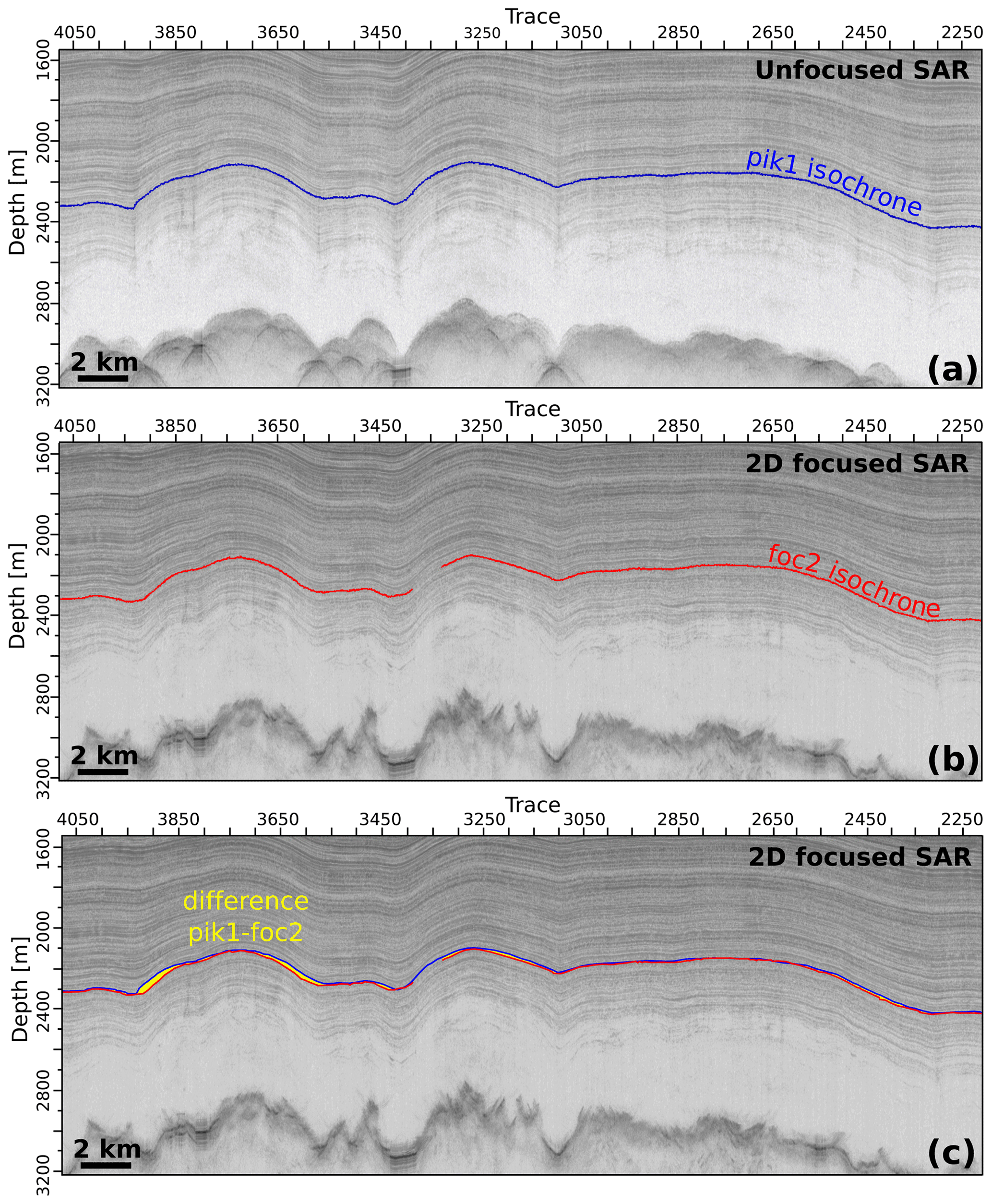
Figure 2 Differences in IRH geometry between different radar processing products: (a) unfocused SAR processed radargram with the corresponding pik1 IRH traced, (b) 2D focused SAR processed radargram with the same IRH traced (foc2) and (c) 2D focused SAR processed radargram with the geometries of the same IRH and their differences plotted as a yellow envelope. Differences are clearly largest where the IRHs are most steeply dipping.

To improve along-track geometries and produce the foc1 and foc2 radar products, we use the matched filter-focusing approach of Peters et al. (2007) by interpolating the data to 1 m records along track and filtering out coherent noise. For foc1, we use focused SAR over the pulse-limited footprint (“1D focusing”) to correct for sub-vertical resolution range variations (delay changes of 100 ns) that change the phase of individual echoes over synthetic apertures of a few hundred meters. This processing results in improved SNR for rough targets but causes loss of subsurface IRHs with slopes >5^∘ (and lower with depth) (Peters et al., 2007). The foc1 processor often produces good results for the bed (particularly in the presence of surface scattering) but is not appropriate for deep IRH tracing (Holschuh et al., 2014). For foc2 (“2D focusing”), we accommodate range variation of up to 1 µs, allowing our matched filter to track echoes for each point for synthetic apertures of over 2 km. By doing so, IRHs with slopes up to 10^∘ can be detected at depth. This processing comes at the expense of increased noise and requires more accurate platform position information (which is sometimes unavailable) and computer time. However, we have found foc2 to be vital for tracking deep IRHs (Fig. 2). Focused SAR is therefore most useful when reflector geometries are complex (e.g., steep slopes), while pik1 is better suited to relatively smooth internal stratigraphy as it has the highest SNR of all processing products. The resulting post-processed radar data characteristics are listed in Table 2.

The IRH data set presented here has been traced using the pik1 unfocused SAR and foc2 2D focused SAR products. These two processing types do not differ much in the Dome C region, due to the exceptionally continuous and relatively flat internal stratigraphy. The biggest differences arise in areas where the IRHs are steeply dipping (Fig. 2), as described by Peters et al. (2007). The foc1 product was not used to trace the IRHs as foc2 provides the best results for tracing sloping IRHs in comparison to foc1. We explicitly state in the published IRH data set which processing type (pik1 or foc2) was used for IRH tracing.

3.2.2 MCoRDS

IRHs were traced on the L1B CSARP-standard product (Arnold et al., 2020; CReSIS, 2016). Processing steps involved in creating the L1B CSARP-standard product are pulse compression in the frequency domain, with a 20 % Tukey window applied in the time domain and a Hanning window applied in the frequency domain; uniform resampling of the data; motion compensation; and finally SAR processing. The SAR processing uses f–k migration with an along-track wavenumber domain Hanning window. The multiple receiver channels are individually SAR processed and then averaged together coherently. Finally, a single image is created by combining the echograms from low (1 µs pulse duration) and high (3 and 10 µs pulse duration) gain channels. The effective along-track beam width is ±5^∘ in ice, which limits the detection of IRH with a dip greater than 5^∘. The resulting post-processed radar data characteristics are listed in Table 2 (Arnold et al., 2020; CReSIS, 2016).

3.2.3 DELORES

After GPS-based precise positioning of the raw DELORES radar data, transects are processed using ReflexW (Sandmeier Geophysics) software. Several filters are applied, in the time and depth domains, to increase the SNR of the IRHs, including suppression of the direct air wave, bandpass filtering, a gain function to correct for spherical spreading loss and migration to collapse diffractions to their source points. The original sampling period of 4 ns is averaged to 12 ns in the post-processed data. Because the collection of ground-based radar data is dependent on the speed of the vehicle, which varies due to the terrain roughness during collection, the radar data are interpolated onto a 5 m regular horizontal spacing during post-processing. The resulting post-processed radar data characteristics are listed in Table 2. The absence of refraction through the air–ice interface allows for very steep IRH slopes to be imaged.

3.3 Internal reflecting horizons (IRHs)

IRHs are interpreted using Landmark's Decision Space Desktop 5000.8.3.0 software. All radar transects are loaded into the software prior to interpretation, and the built-in basemap is used to track the same IRH continuously from one transect to the next through the use of crossover points (Fig. 3). Prior to loading, the radar transects are flattened to the surface, which is itself set at zero two-way travel time (TWTT) so that surface echoes and internal stratigraphy match between systems and IRHs can be reliably traced across cross-cutting transects. At each crossover point, the software indicates the TWTT of the IRH traced while the 2D viewer allows the visualization of the intersecting radar transects side-by-side to ensure the traced IRH is continuous across the intersection.

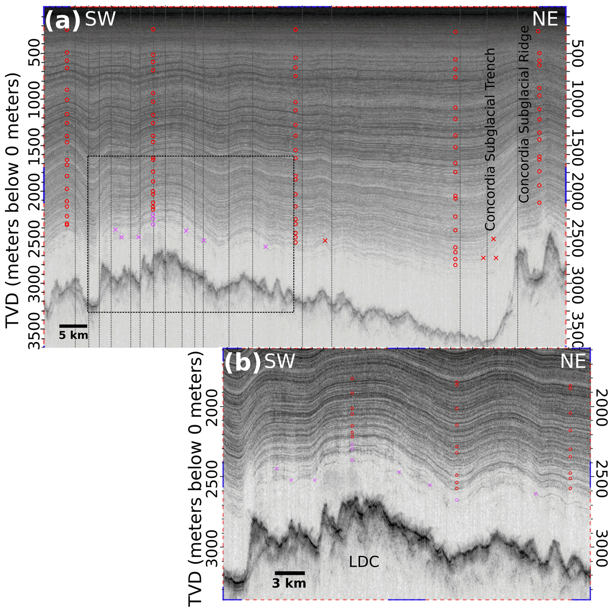
Figure 3 Radargram showing the depth distribution of the IRHs. (a) The full transect displayed here (OIA/JKB2n/X57a) starts over the LDC and crosses over the Concordia Subglacial Trench and Ridge, where the deepest IRHs cannot be traced across (transect is indicated in Fig. 1). Red and magenta circles highlight the dated and undated IRHs, respectively (see Sect. 3.4.2 for definitions), and red and magenta crosses indicate where each IRH tracing is interrupted. Crossing transects are indicated by dashed vertical black lines. (b) Detailed view of the bottom half of the ice column over LDC, where the undated IRHs are most densely traced, although they end quite quickly with distance from the LDC bedrock high.

To trace the IRHs, we use Decision Space Desktop's semi-automated tracking algorithm to track peaks in the radargram echo amplitudes. This algorithm has a travel-time-adjustable window that can be adjusted as a function of the local roughness of the specific IRH being traced. Traced IRHs are chosen based on their brightness and continuity. A traced IRH can start off looking bright and easy to follow but due to various processes (e.g., wind redistribution of surface snow which then gets buried, enhanced ice flow) can get truncated further along a survey transect. Such IRHs are abandoned and only those that could cover >50 % of the whole Dome C region were retained and are published in this data set. The deepest IRHs are truncated on a few radar transects that were flown over steep bedrock topography. This geometry creates steeply dipping IRHs which are difficult to recover in the post-processed data. For HiCARS transects, the type of processing applied (pik1 or foc2) affects the geometry of the IRH. If both types of processing are available for the same transect (this is especially the case for the OIA survey), the IRH is traced separately both in pik1 and in foc2, and each version is then considered as a separate data set.

In using several radar systems, there is the added difficulty of tracing IRHs reliably from one radar system to the next at crossover points (Cavitte et al., 2016; Winter et al., 2019). Cavitte et al. (2016) have shown that transferring IRHs from the HiCARS system to the MCoRDS system is achievable, despite the differences in their range resolutions. Because MCoRDS has a finer range resolution (4.30 m for MCoRDS vs. 8.42 m for HiCARS), some of the IRHs selected in the HiCARS radargrams correspond to two IRHs on the MCoRDS radar transect (Fig. 4, panel a). However, Cavitte et al. (2016) show that the IRHs can be traced over hundreds of kilometers and still match between the two radar systems within their age uncertainty ranges. Similarly, Winter et al. (2019) show that their IRHs, traced using the Alfred Wegener Institute (AWI) radar system with a 50 ns pulse source waveform and a range resolution of 5 m, can be matched to the HiCARS IRHs presented in this data release. Similarly, tracing the IRHs across from the airborne-collected HiCARS radar data to the ground-based DELORES radar data is also tractable, with a difference in range resolution of 2.85 m (8.42 m vs. 11.09 m). Figure 4, panel b, shows a good one-to-one match in the IRHs. The 26 IRHs can be traced through all of the DELORES radar transects presented here.

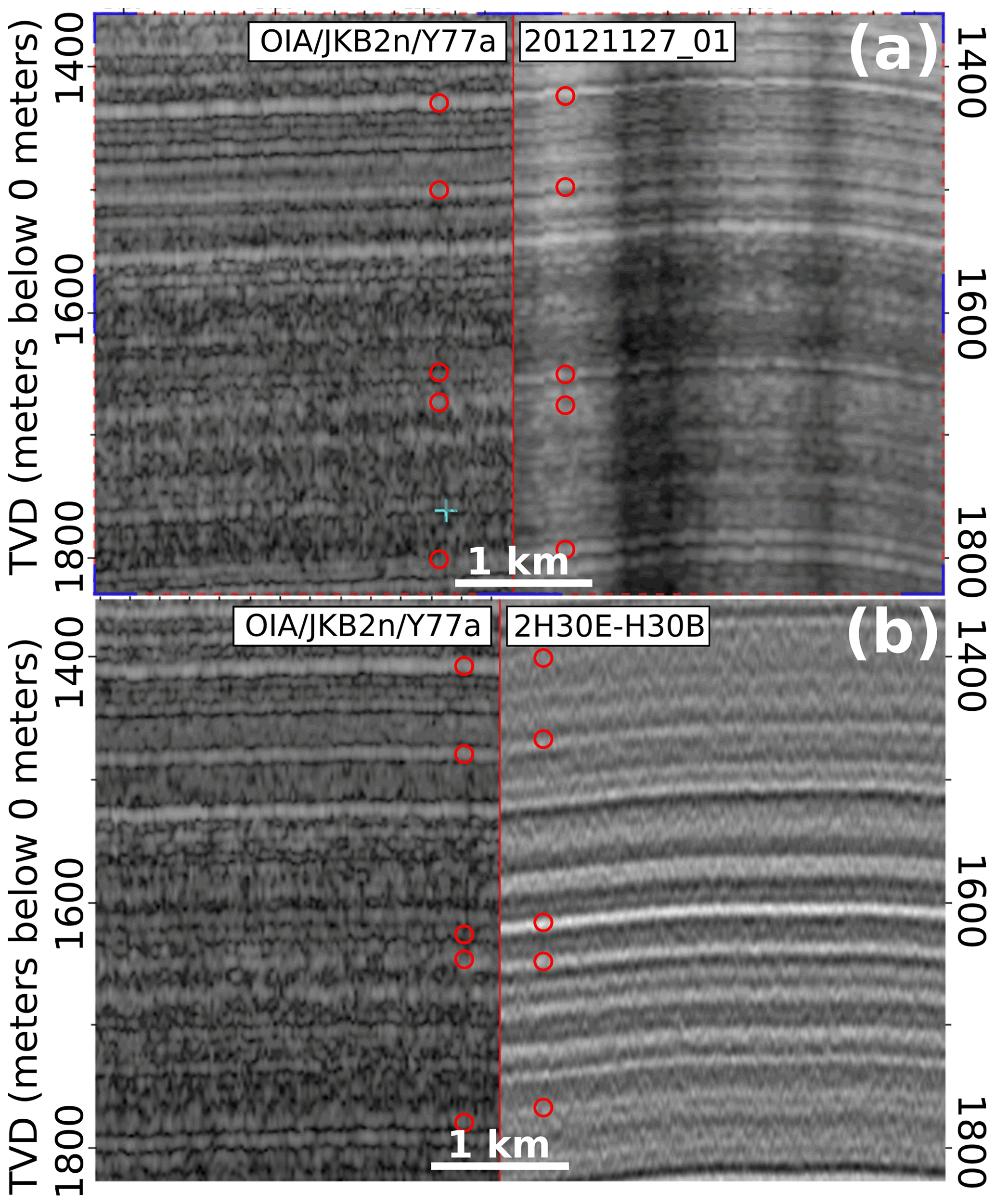
Figure 4 Zoomed-in view of radar transect intersections between different radar systems: (a) between the HiCARS OIA transect OIA/JKB2n/Y77a and the DELORES transect 2H30E-H30B (both marked in Fig. 1) and (b) between the HiCARS OIA transect OIA/JKB2n/Y77a and the MCoRDS transect 20121227_01 (red line in Fig. 1). The traced IRHs are highlighted by red circles either side of the crossover point (marked by a red vertical line). The vertical scale is the true vertical depth (TVD) in meters. Note that in this color map, IRHs (maximum amplitudes in radar returns) are displayed in white.

The dense coverage of the ice-penetrating radar data in the Dome C region means that all radar transects used are directly connected at multiple crossovers. This implies that IRHs can be reliably extended across the whole region by transferring from one profile to the next using matching TWTT at the crossover points. This also allows us to perform a check on the IRH tracing and confirm the isochroneity of the chosen IRHs.

3.4 IRH depth and age attribution

3.4.1 Depth attribution

One of the HiCARS survey lines (MCM/JKB1a/EDMC01a) passes very close to the EPICA Dome C (EDC) ice core site (Fig. 1), with a gap of 94 m between the ice core site and the point of closest approach. At this point, the IRH depths can be calculated from their TWTT according to the following equation (e.g., Steinhage et al., 2001; MacGregor et al., 2015; Cavitte et al., 2016; Winter et al., 2019):

$$\begin{array}{}\text{(3)}& z_{\mathrm{IRH}}={\displaystyle \frac{\text{TWTT}{C}_{\mathrm{air}}}{\mathrm{2}\sqrt{\mathit{ϵ}{{}^{\prime }}_{\mathrm{ice}}}}}+z_{\mathrm{f}},\end{array}$$

where the electromagnetic velocity in air (C_air) is 300 m µs⁻¹, $\mathit{ϵ}{{}^{\prime }}_{\mathrm{ice}}$ is the relative dielectric permittivity of ice and z_f is the firn correction. We use an $\mathit{ϵ}{{}^{\prime }}_{ice}=\mathrm{3.17}$ (Gudmandsen, 1971; Peters et al., 2005) and a firn correction =14.60 m following Cavitte et al. (2016), calculated from Eq. (4) in Dowdeswell and Evans (2004) and the Barnes et al. (2002) EDC density profile. Since all our IRHs are below the firn transition, temperature and ice fabric variations have a small effect; i.e., we can ignore variations in $\mathit{ϵ}{{}^{\prime }}_{ice}$ with depth and use a constant value. However, variations in $\mathit{ϵ}{{}^{\prime }}_{ice}$ are taken into account to quantify the IRH depth uncertainties (see Sect. 3.5 below).

3.4.2 Age attribution

Using the IRH depths measured at the closest point to the ice core site, we can assign ages to the IRHs using the AICC2012 chronology (Bazin et al., 2013; Veres et al., 2013). We linearly interpolate the age–depth chronology to match our IRH depths and date the IRHs. Hereinafter, we refer to these as the “dated IRHs”. Note that we use a deterministic approach to date the IRHs; however a Bayesian approach, such as used in Muldoon et al. (2018), could also be applied to the IRH data.

IRHs that cannot be traced all the way to radar transect MCM/JKB1a/EDMC01a (Fig. 1 and Cavitte et al., 2016), due to stratigraphic discontinuity or radar image quality issues, cannot be assigned ice core ages. We refer to these IRHs explicitly as “undated IRHs”. As a result of their isochronal nature, these undated IRHs represent informative stratigraphic constraints that can be useful in modeling efforts, and we therefore include them in this data release. We can however provide an estimate of the age of these “undated IRHs” using the 1D pseudo-steady (Parrenin et al., 2006) ice flow model described in Parrenin et al. (2017). We use the dated IRHs as age and depth constraints to calculate a steady-state age–depth modeled field for each radar transect. The ages simulated for the bottom ∼20 % of the ice sheet, i.e., older than the deepest dated IRH, are therefore extrapolated ages. From the measured undated IRHs depths, we sample the simulated age–depth field and assign a modeled age to every trace along the radar transects (Fig. 8). We can then assign a mean modeled age for each undated IRH.

3.5 IRH uncertainty quantification

3.5.1 Depth uncertainties

Cavitte et al. (2016) list the three main sources of depth uncertainty for IRHs. The first source of depth uncertainty comes from the vertical resolution of the radar system used, provided in Table 2 for each radar system. For chirp systems, by definition, range resolution Δr is given by $\mathrm{\Delta }r=C_{\mathrm{ice}}/\left(\mathrm{2}B\right)$, where B is the bandwidth of the radar system, or equally $\mathrm{\Delta }r=\left(C_{\mathrm{ice}}{p}_{\mathrm{w}}\right)/\mathrm{2}$, where p_w is the effective pulse duration. In the case of the CReSIS system, because of the 20 % Tukey time-domain window and Hanning frequency-domain window applied, range resolution is given by CReSIS (2016) as $\mathrm{\Delta }r=\left(k_t{C}_{\mathrm{ice}}\right)/\left(\mathrm{2}B\right)$, where k_t=1.53 is the window widening factor computed numerically to find the pulse width 3 dB down from the peak. For a signed, low-frequency waveform, as found in DELORES radargrams, the above rule does not apply, and for range resolution we instead use $\mathrm{\Delta }r={\mathit{\lambda }}_{\mathrm{ice}}/\mathrm{4}$, where λ_ice is the wavelength of the signal in ice. Following Cavitte et al. (2016), since we are interested in identifying individual specular returns in the ice, by measuring the SNR of each IRH at the ice core site, we can calculate the range precision, σ_r, of each IRH according to

$$\begin{array}{}\text{(4)}& {\mathit{\sigma }}_{\mathrm{r}}={\displaystyle \frac{\mathrm{\Delta }r}{\sqrt{\text{SNR}}}},\end{array}$$

with SNR given on a linear scale. Range precision is improved over range resolution for an IRH with a SNR >1. Note that the range precision calculated is valid at the EDC site but might not be constant laterally, since IRH SNR varies spatially. However, we assume it provides a representative value of the “real” σ_r value for each IRH. This range precision calculation assumes a single resolved target, and the precision could be worse if two or more IRHs of comparable power are present.

A second source of uncertainty comes from measurement errors in the depth–density curves used to calculate the firn correction. We use a depth error of ±1.35 m at the EDC site as described in Cavitte et al. (2016), based on the Barnes et al. (2002) published measurement errors.

A third source of uncertainty comes from the variations in the dielectric permittivity $\mathit{ϵ}{{}^{\prime }}_{\mathrm{ice}}$ as a function of temperature, impurity concentration and anisotropy (Peters et al., 2005; Fujita et al., 2000), which affects the calculated IRH depths. Electromagnetic velocities in ice vary between 168 and 169.5 m µs⁻¹ (Fujita et al., 2000), which increases the uncertainty in the depth calculations with depth. For the deepest dated IRH traced (366 ka), this represents a maximum depth error of ±11.65 m at the EDC site.

The total depth uncertainty is the root-sum-square error of each of these three uncertainties. It is calculated for each dated IRH and listed in Table 3.

Table 3 Depths, ages and uncertainties of the 19 dated IRHs, measured and calculated at the EDC site, using the AICC2012 chronology (Bazin et al., 2013; Veres et al., 2013). Δz and Δa stand for depth and age uncertainty, respectively.

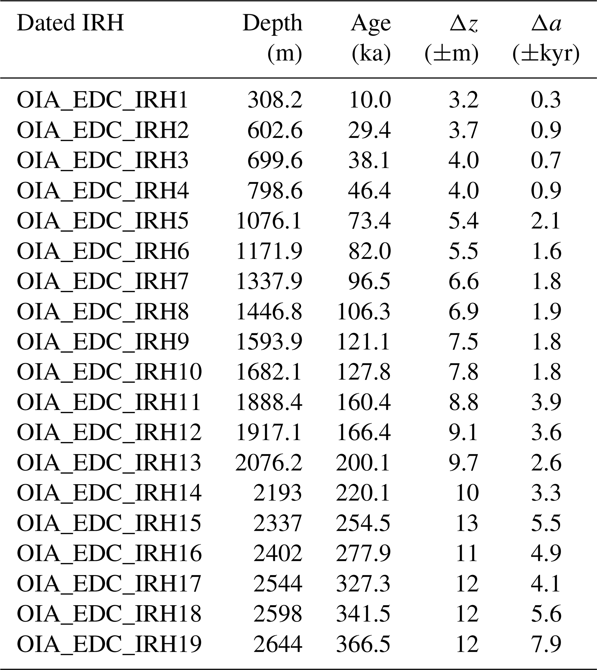
Note that values have been updated since Cavitte et al. (2016).

Additional, but not quantified, sources of uncertainty come from (1) the assumption of horizontal continuity of the IRHs between the EDC site and the radar transect, which corresponds to a distance of ∼94 m; (2) the complexity of tracing the same IRH across two radar transects from different systems (discussed in Sect. 3.3); (3) vertical advection over the 10 years of data collection, although, considering the radar resolutions (4.30 m minimum) and the surface accumulation rate (∼25 mm yr⁻¹, Stenni et al., 2016), we assume that this factor can be neglected; and (4) the assumption that only a single target is present in the range precision estimate for the IRH.

Depth uncertainties are also assigned to the undated IRHs (Table 4). Since these IRHs do not reach the MCM/JKB1a/EDMC01a transect, their depths are measured at the closest point along the DELORES radar transect HRB7-HRB8 to the final chosen BE-OI drill site BELDC (75.29917^∘ S, 122.44516^∘ E) (Lilien et al., 2021), and their uncertainties are constrained as described above but with their range precision defined by their SNR along this DELORES transect. We assume that the firn correction and error calculated at the EDC site are also applicable to this site over LDC.

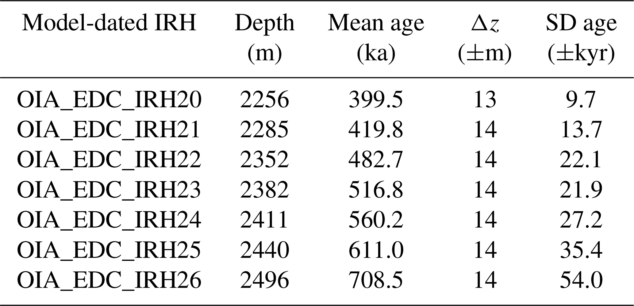
Table 4 Depths and modeled mean ages for the seven model-dated IRHs, using the Parrenin et al. (2017) 1D steady-state ice flow model. Depths are measured at the closest point along the DELORES radar transect HRB7-HRB8 to the final BELDC drill site (measured local ice thickness of ∼2747 m), and depth uncertainties are calculated as described in Sect. 3.5 for that same location along transect HRB7-HRB8. Age uncertainties here are mostly representative of the model age uncertainty: they are calculated as the standard deviation of the spatial distribution of the age of each IRH.

3.5.2 Age uncertainties

The total age uncertainty of an IRH results from the combination of the published ice core age uncertainty, Δa_Δcore (Bazin et al., 2013; Veres et al., 2013), and the IRH's depth uncertainty, Δa_Δz (described above). The depth uncertainty is converted to an age uncertainty using the AICC2012 chronology to calculate the local age gradient for each IRH depth. These two sources of uncertainties are combined as a root-sum-square error as in Cavitte et al. (2016) and Winter et al. (2019):

$$\begin{array}{}\text{(5)}& \mathrm{\Delta }a=\sqrt{\mathrm{\Delta }{a}_{\mathrm{\Delta }z}^{\mathrm{2}}+\mathrm{\Delta }{a}_{\mathrm{\Delta }\mathrm{core}}^{\mathrm{2}}}.\end{array}$$

Combined age uncertainties (Δa) calculated for each dated IRH are summarized in Table 3.

4 Results

In total, 26 IRHs are traced across the wider Dome C region, using the 79 radar transects, representing >15 500 km of IRH data interpreted over this part of the East Antarctic Plateau (Fig. 1, Cavitte et al., 2020). Of these 26 IRHs, 19 IRHs are dated. These dated IRHs span four glacial cycles, from the shallowest IRH dated at ∼10 ka to the deepest IRH dated at ∼366 ka. The depths and ages, as well as the uncertainties associated, of the dated IRHs are summarized in Table 3, and their temporal spread is displayed in Fig. 5. Figure 6 shows, for each dated IRH, the depth anomaly of the dated IRH with respect to its average depth from the ice surface, as a percentage anomaly. It shows where the IRH is deeper or shallower locally than on average.

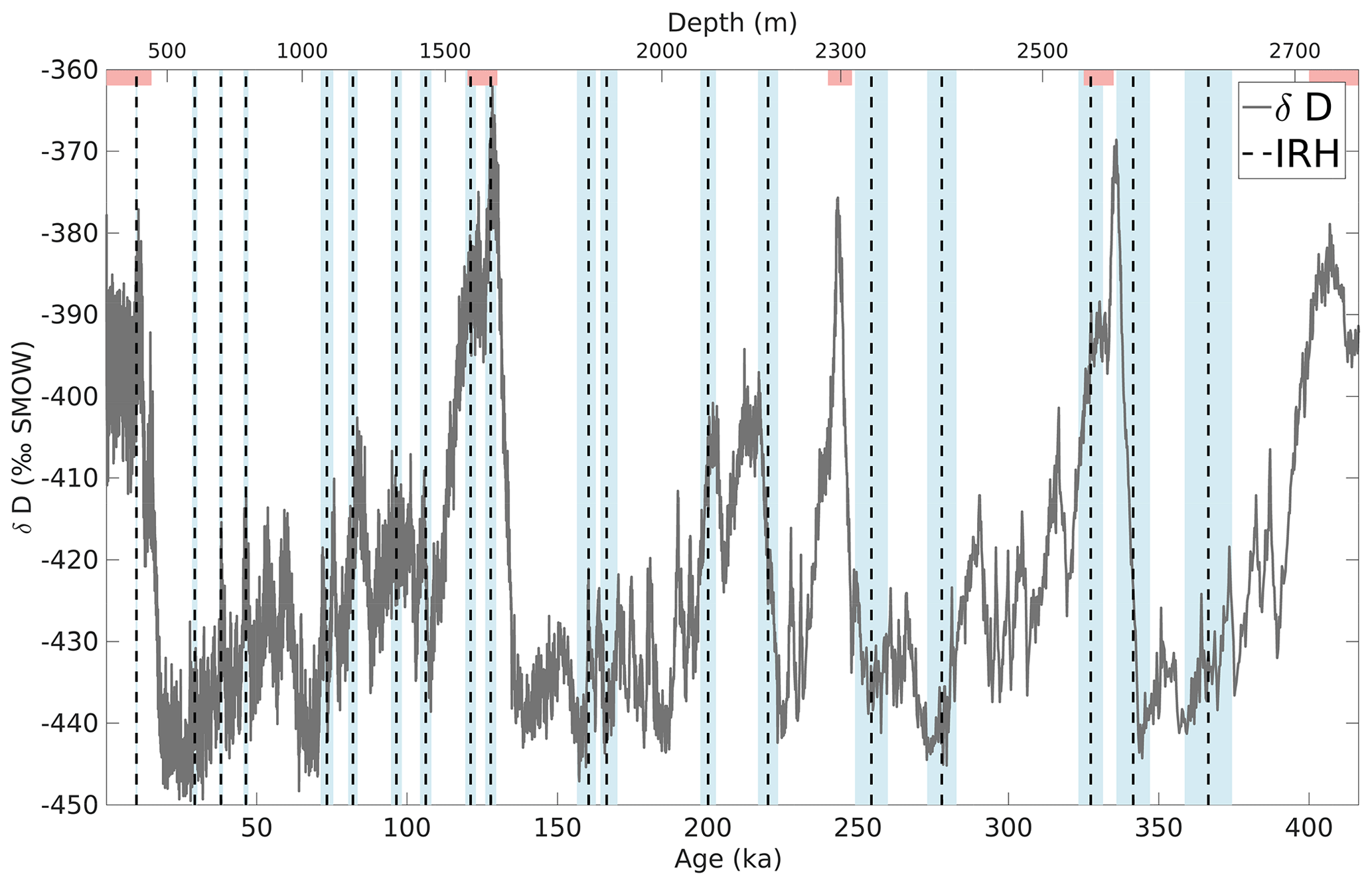
Figure 5 Temporal coverage of the dated IRHs (as dashed black vertical lines) over the past four glacial cycles, here displayed on top of δD variations in per mil Standard Mean Ocean Water (SMOW) measured on the EDC ice core and using the AICC2012 chronology (Bazin et al., 2013). IRH age uncertainties are indicated by light blue shading. Red bars highlight the interglacial periods for reference.

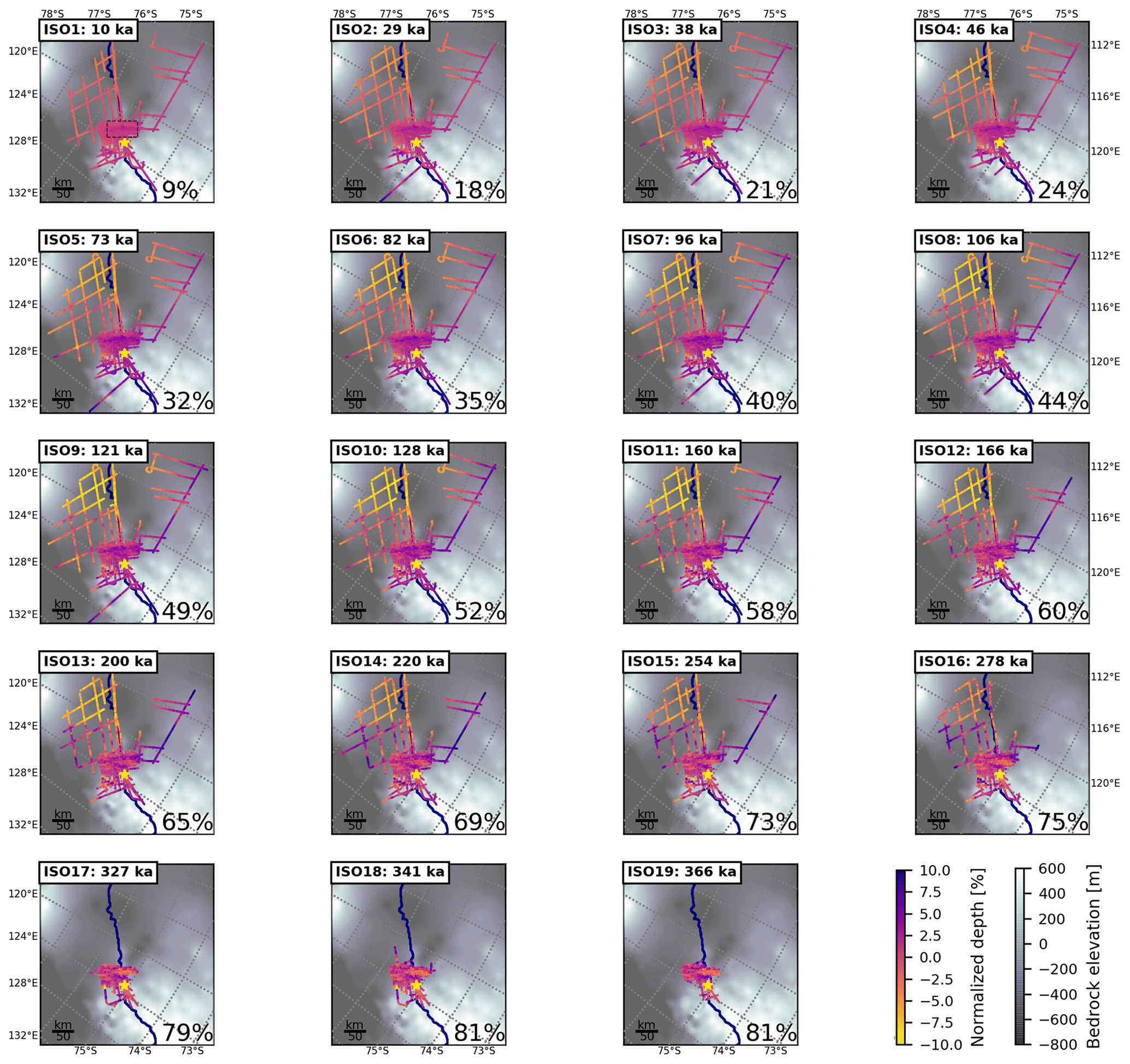
Figure 6 Spatial distribution of dated IRH depths over the Dome C region of the East Antarctic Plateau, overlain on BedMachine Antarctica v1 bedrock topography (Morlighem et al., 2020) for context. The color scale represents the percent depth anomaly of the IRH from its average percent depth (marked in the bottom right corner of each panel): darker colors imply that the IRH is deeper locally than on average, and lighter colors imply that the IRH is shallower locally than on average. Percent depths are normalized by the ice thickness, both measured from the radar returns (HiCARS, MCoRDS or DELORES). The yellow star locates the EDC ice core site, and the navy blue line outlines the position of the ice divide (Zwally et al., 2012). A black dashed box on the first panel outlines the LDC highland area covered by Figs. 7 and 8.

Characteristics of internal stratigraphy

The LDC is a region where the combination of the very flat internal stratigraphy (due to the low surface velocities) and very cold surface conditions ($\sim -\mathrm{54.5}$ ^∘C on average year-round, EPICA commmunity members, 2004) results in good preservation of the internal stratigraphy and therefore all 19 dated IRHs continuously traced over the whole area. As we step off the LDC bedrock plateau, the deepest IRHs become difficult to trace (in particular the bottom three). Affected by the presence of the deep Concordia Subglacial Trench on the northeast side (∼600 m cliff) and the Aurora Subglacial Basin on the southwest side, the IRHs steepen, with the strongest impact on the deepest ones. We observe a gradient, consistent for all dated IRHs, of depth shallowing from the north side of Dome C to its south side. This has been observed previously (Urbini et al., 2008; Verfaillie et al., 2012; Cavitte et al., 2018; Le Meur et al., 2018; Frezzotti et al., 2005) and results from the accumulation gradient at the surface with average moisture provenance from the Indian Ocean moving across the ice divide (Scarchilli et al., 2011). Although the deepest dated IRH reaches on average 81 % of the ice thickness, with local maxima of ∼90 %, its age of 366 ka represents only ∼45 % of the total age interval measured at EDC.

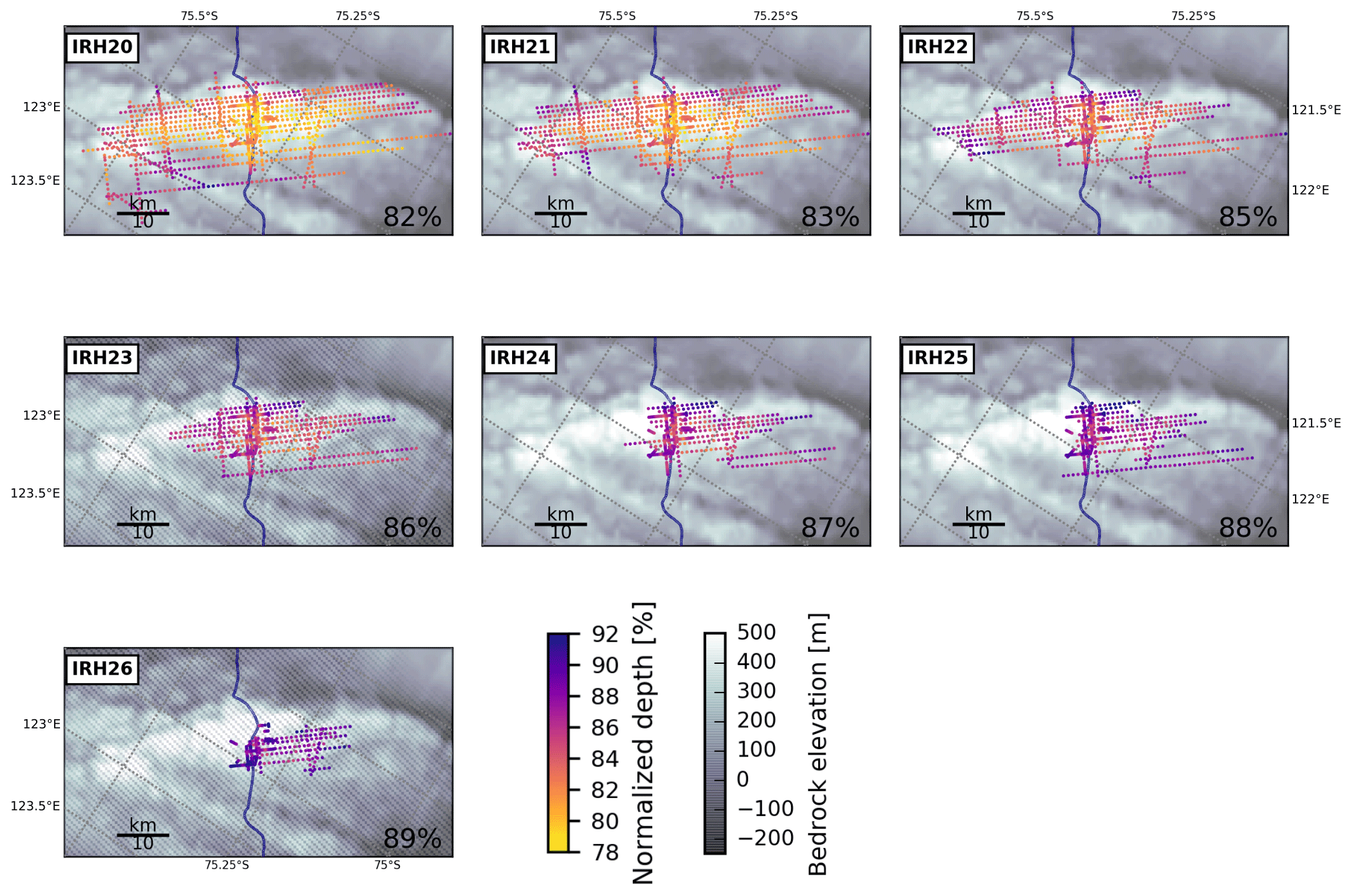
Figure 7 Spatial distribution of undated IRH depths over the LDC highland plateau on the East Antarctic Plateau, overlain on Young et al. (2017) bed elevations. The area covered by each panel is outlined by a black dashed box in the first panel of Fig. 6. The color scale represents the depth of the IRHs normalized by the ice thickness, both measured from the radar returns. The navy blue line outlines the position of the ice divide (Zwally et al., 2012).

Of the 26 IRHs traced in the Dome C region, seven IRHs remain undated. The seven undated IRHs are also the deepest IRHs. The difficulty in connecting them to the MCM/JKB1a/EDMC01a (Fig. 1) radar transect stems from their proximity to the bedrock, which induces strongly dipping internal geometries that become difficult to track continuously. We plot the depth distribution of all seven undated IRHs (Fig. 7), which are much less extensive than the dated IRHs and are constrained to the LDC highland region. We can see that the deepest undated IRH reaches on average ∼89 % depth of the ice thickness, with local maxima reaching 90 %–92 %, relatively close to the bedrock.

Figure 8 Spatial distribution of modeled ages for the seven bottom IRHs over the Dome C region of the East Antarctic Plateau, overlain on Young et al. (2017) bed elevations. The area covered by each panel is outlined by a black dashed box in the first panel of Fig. 6. The color scale represents the predicted age of the model-dated IRHs, interpolated from the modeled age–depth field. The navy line outlines the position of the ice divide (Zwally et al., 2012).

We use the 1D pseudo-steady ice flow model (Parrenin et al., 2006, 2017) and the above 19 dated IRHs to assign a mean age to the undated IRHs, as well as the age standard deviation, based on their modeled spatial age distribution (Table 4). The deepest IRH, with a modeled age of 709 ka, has an average depth of 89 % over its whole extent and reaches 90 % of the ice thickness at the closest point to the final chosen BELDC drill site. This implies a severe age gradient in the bottom ∼10 % of the ice locally, with strong implications for resolving the climate signal of the deep ice core to be recovered.

5 Discussion

We were able to map the internal stratigraphy extensively throughout the Dome C plateau region as a result of the good glaciological conditions for ice-penetrating radar imaging: slow ice flow velocities in the region, cold surface temperatures year-round ($\sim -\mathrm{54.5}$ ^∘C on average, EPICA commmunity members, 2004, and therefore absence of melting at the surface) and the lack of any (known) history of paleo flow direction switches. All these factors combine to create smooth, continuous and bright IRHs that can be traced over very long distances. Siegert et al. (1998a) were already able to trace IRHs in the vicinity of Dome C without encountering continuity issues. Difficulties mostly arose in approaching the Vostok ice core site, located ∼550 km away, due to wind-driven snow redistribution buried beneath the surface, as well as the advected accumulation high over the Vostok Lake (Leonard et al., 2004; Cavitte et al., 2016).

In the data set published here (Cavitte et al., 2020), we observe no obvious signs of disruptions in the englacial stratigraphy. This is consistent with the Das et al. (2013) distribution of glazed areas and known megadune areas (Frezzotti et al., 2005; Arcone et al., 2012), which show no overlap. Most difficulties in tracing IRHs arise for the deepest IRHs (Fig. 3). Robin and Millar (1982) first described how the effect of the bedrock topography has the strongest impact on the internal stratigraphy immediately above the bed and decreases with distance from the bed, while modeling efforts have brought to light the influence of basal processes on internal stratigraphy. Variations in basal geothermal heat flux, the presence or absence of basal lubrication, or the roughness of the bedrock topography can cause the folding or the down- or up-draw of the IRHs, which all complicate the continuous tracing of their geometries (e.g., Leysinger Vieli et al., 2011; Leysinger-Vieli et al., 2018). This increasing complexity of the IRH geometries is obvious, even visually, in the IRHs presented here (Fig. 3). Because the deepest IRHs are generally the steepest, their coverage is spatially limited (Fig. 8). Holschuh et al. (2014) have shown how the different types of radar processing can create destructive interference in the case of steeply dipping surfaces in the along track direction; similarly, reflections from surfaces dipping across track can be nulled by the across track antenna beam pattern structure. This is particularly true, for example, across the Concordia Subglacial Trench. Here, the 600 m trench, followed by the 600 m cliff of the Concordia Ridge, has a strong effect on the IRH geometries (Fig. 3, Parrenin et al., 2017; Passalacqua et al., 2018). Furthermore, the ice becomes warmer the closer it gets to the bed as a result of the thick insulating ice above and the conduction of geothermal heat from below (Pattyn, 2010; Van Liefferinge and Pattyn, 2013). Temperature affects the dielectric permittivity of the ice and can result in a strongly attenuated radar return and a lower SNR of the IRHs (Matsuoka, 2011; MacGregor et al., 2012).

Note that there is now evidence that there is a layer of ice just above the bed, and in particular over the LDC highland plateau, with different electromagnetic properties, which is assumed could be stagnant (Young et al., 2017; Cavitte, 2017; Lilien et al., 2021). The Parrenin et al. (2017) ice flow model version used does not take this stagnant ice into account, which could make the basal ages, and therefore the seven bottom IRHs, too young in the present modeling. A new version of the 1D model that takes into account this stagnant layer has been developed, and it will be interesting to compare the new ages obtained (Fred Parrenin, personal communication, 2020).

The formulated goal of the AntArchitecture action group is to have a joint community effort to build an Antarctic-wide IRH data set to check the match between all previously traced and published IRH data sets that can be directly connected for the East Antarctic Plateau region (to name a few, Siegert et al., 1998a; Winter et al., 2019). Eventually, the aim is that IRHs from currently disconnected surveys (e.g., Steinhage et al., 2001; Leysinger Vieli et al., 2011; Steinhage et al., 2013) are also connected after the collection of additional radar campaigns in the gap areas. The Greenland Ice Sheet already benefits from an ice-sheet-wide IRH data set (MacGregor et al., 2015). For Greenland, it is a huge advantage to have significant coverage from the same system. Antarctica has the challenge of being bigger and more remote, and the existing data sets have been collected for decades using many different systems. However, several studies have already demonstrated this is achievable at the scale of the West Antarctic Ice Sheet (Muldoon, 2018; Ashmore et al., 2020; Bodart et al., 2021). Models have been integrating IRH data for decades, but until now, most of the surveys used had been local (a few square kilometers to a few ice catchments in size) (e.g., Koutnik et al., 2016; Beem et al., 2018; Drews et al., 2015). As the radar data sets become more spatially extensive, different problems can be tackled (e.g., Medley et al., 2013; Muldoon, 2018; Sutter et al., 2021).

6 Code and data availability

The IRHs presented in this study can be found publicly on the US Antarctic Program Data Center (USAP-DC): https://doi.org/10.15784/601411 (Cavitte et al., 2020). The code for the 1D steady-state ice flow model is available publicly at https://github.com/parrenin/IsoInv (last access: 1 September 2017, Parrenin, 2017). The CReSIS radargrams can be accessed at https://data.cresis.ku.edu/data/rds/2013_Antarctica_P3/CSARP_standard/20131127_01 (last access: 1 September 2020, CReSIS, 2020), the HiCARS radargrams can be accessed at https://doi.org/10.26179/5wkf-7361 (Young et al., 2021), https://doi.org/10.5067/W2KXX0MYNJ9G (Blankenship et al., 2017), and the DELORES profiles discussed in this paper will be available from https://data.bas.ac.uk (last access: 14 October 2021, BAS, 2020). The AntArchitecture action group can be found at https://www.scar.org/science/antarchitecture/home/ (last access: 1 September 2020, SCAR, 2020).

7 Conclusions

We traced 26 IRHs across the Dome C plateau region, including 19 that could be dated at the EDC site, and another seven undated IRHs, constrained to the LDC highland area. We publish this internal stratigraphy data set in a long-term data repository (Cavitte et al., 2020) with the associated depth and age uncertainties of each IRH. The dated IRHs span the last four glacial cycles, the youngest dated at 10±0.25 ka and the oldest dated at 366±5.78 ka. The bottom seven IRHs are provided with ages using a 1D inverse model, which indicate an oldest predicted age of ∼709 ka. In this region of the East Antarctic Plateau, the biggest limitation in the tracing of the deep IRHs is their proximity to the rugged bedrock that induces both dipping geometries and attenuated radar returns due to higher basal ice temperatures and thus lower SNR. Nevertheless, at the LDC highland region near Dome C, we are able to trace IRHs down to a depth of ∼89 % of the ice thickness. This data set was used to corroborate suspicions of 1.5 million-year-old ice in the Little Dome C region (Van Liefferinge and Pattyn, 2013; Parrenin et al., 2017) and will also provide the basis for a regional assessment of age at depth for other planned deep drillings in this region (e.g., Australia).