the Creative Commons Attribution 4.0 License.
the Creative Commons Attribution 4.0 License.
 | 11 Aug 2021
A global total column ozone climate data record
Greg E. Bodeker
Jan Nitzbon
Jordis S. Tradowsky
Stefanie Kremser
Alexander Schwertheim
Jared Lewis
Total column ozone (TCO) data from multiple satellite-based instruments have been combined to create a single near-global daily time series of ozone fields at 1.25∘ longitude by 1∘ latitude spanning the period 31 October 1978 to 31 December 2016. Comparisons against TCO measurements from the ground-based Dobson and Brewer spectrophotometer networks are used to remove offsets and drifts between the ground-based measurements and a subset of the satellite-based measurements. The corrected subset is then used as a basis for homogenizing the remaining data sets. The construction of this database improves on earlier versions of the database maintained first by the National Institute of Water and Atmospheric Research (NIWA) and now by Bodeker Scientific (BS), referred to as the NIWA-BS TCO database. The intention is for the NIWA-BS TCO database to serve as a climate data record for TCO, and to this end, the requirements for constructing climate data records, as detailed by GCOS (the Global Climate Observing System), have been followed as closely as possible.
This new version includes a wider range of satellite-based instruments, uses updated sources of satellite data, extends the period covered, uses improved statistical methods to model the difference fields when homogenizing the data sets, and, perhaps most importantly, robustly tracks uncertainties from the source data sets through to the final climate data record which is now accompanied by associated uncertainty fields. Furthermore, a gap-free TCO database (referred to as the BS-filled TCO database) has been created and is documented in this paper. The utility of the NIWA-BS TCO database is demonstrated through an analysis of ozone trends from November 1978 to December 2016. Both databases are freely available for non-commercial purposes: the DOI for the NIWA-BS TCO database is https://doi.org/10.5281/zenodo.1346424 (Bodeker et al., 2018) and is available from https://zenodo.org/record/1346424. The DOI for the BS-filled TCO database is https://doi.org/10.5281/zenodo.3908787 (Bodeker et al., 2020) and is available from https://zenodo.org/record/3908787. In addition, both data sets are available from http://www.bodekerscientific.com/data/total-column-ozone (last access: June 2021).
- Article
(20897 KB) - Full-text XML
- BibTeX
- EndNote


Total column ozone (TCO) has been identified as one of 50 essential climate variables (ECVs) by GCOS (Global Climate Observing System; GCOS-138, 2010; Bojinski et al., 2014). Climate data records of ECVs serve a variety of purposes; e.g. climate data records of TCO are required to (1) assess the impacts of changes in ozone on radiative forcing of the climate system, (2) assess the effectiveness of the Montreal Protocol for the protection of the ozone layer, and (3) determine the contribution of ozone changes to observed long-term trends in surface UV radiation. This paper presents an update of a database which has been used in many previous studies (e.g. Bodeker et al., 2001a, b, 2005; Müller et al., 2008). The database was first developed by NIWA (the New Zealand National Institute of Water and Atmospheric Research) and, in the last decade, has been maintained and updated by Bodeker Scientific (BS). The non-filled database is hereafter referred to as the NIWA-BS TCO database and the filled database is referred to as the BS-filled TCO database. The version 3.4 (V3.4) database reported on here extends from 31 October 1978 to 31 December 2016. In constructing this database, the guidelines for generating climate data records of ECVs detailed in GCOS-143 (2010) have been adhered to.
Improvements over earlier versions of the database implemented in V3.4 include the following:
-
New and updated sources of satellite-based TCO measurements are used, namely data from NPP-OMPS (National Polar-orbiting Partnership-Ozone Mapping and Profiler Suite), GOME-2 (Global Ozone Monitoring Experiment-2), and SCIAMACHY (Scanning Imaging Absorption Spectrometer for Atmospheric CHartographY) are now included in the combined data set. Various updates to previously used data sets are detailed in Sect. 2.
-
Improved statistical methods are used to model the difference fields between data sets; zonal means of the difference fields are modelled using Legendre expansions which comprise the meridional component of a spherical harmonic expansion which is best suited for statistically describing a field on a sphere (see Sect. 3 for more information).
-
Measurement uncertainties on the source data sets, and the corrections applied to those data sets, have been collated and are propagated through to the combined ozone data set so that, for the first time, this data set is now provided with uncertainty estimates for each datum.
-
Furthermore, the gap-free BS-filled TCO database has been generated (see Sect. 9) using a machine-learning (ML) algorithm that is trained to capture the broad-scale morphology of the TCO field which extends to regions where measurements are missing. The ML algorithm is based on regression of available data against NCEP (National Centers for Environmental Prediction) CFSR (Climate Forecast System Reanalysis) reanalysis tropopause height fields and against potential vorticity (PV) fields on the 550 K surface.
The various satellite-based TCO data sets used to create the version 3.4 NIWA-BS TCO database are summarized in Table 1. Where source data were provided at resolution, bilinear interpolation was used to resample the data to resolution. The time periods covered by the satellite data sets are shown graphically in Fig. 1.
Table 1The source data sets used to create version 3.4 of the NIWA-BS TCO database.
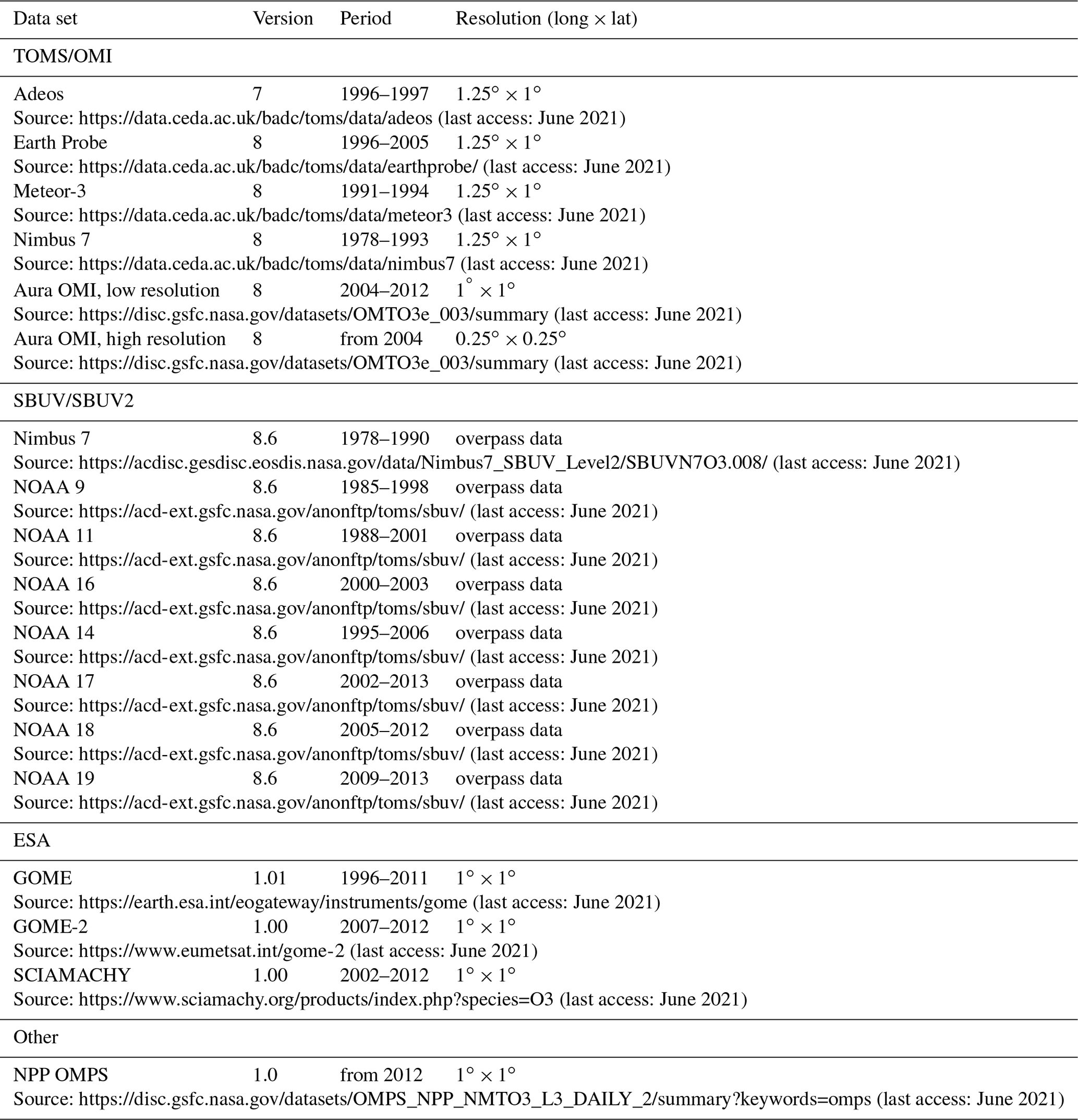

Figure 1A graphical representation of the different satellite-based data sets used in this study and their periods of coverage. Satellites marked with a dashed line indicate newly added source data for this version of the database.
In addition to the information presented in Table 1:
-
The four TOMS (Total Ozone Mapping Spectrometer) data sets (Adeos, Earth Probe, Meteor 3, and Nimbus 7) all use the TOMS retrieval algorithm with Adeos using the version 7 algorithm and the remaining three using the version 8 algorithm.
-
An algorithm similar to that used in the version 8 TOMS retrieval is used to conduct the version 8.6 retrievals of the SBUV (Solar Backscatter UltraViolet instrument) data (McPeters et al., 2013). Sparse gridded files were generated from the SBUV TCO measurements made at discrete locations as input to the process that creates the combined database.
-
The high-resolution and low-resolution OMI (Ozone Monitoring Instrument) data sets both use a TOMS-like (version 8) retrieval algorithm.
-
The GOME, GOME-2, and SCIAMACHY data sets all use the GOME Direct Fitting (GODFIT) retrieval algorithm (Lerot et al., 2010).
-
As stated in Sect. 1.1 of the OMPS Algorithm Theoretical Basis Document (ATBD), the algorithm used for retrieving the OMPS TCO is adapted from the heritage TOMS version 7 retrieval.
First, the corrections required to the TOMS and OMI data sets are determined by comparing the satellite-based measurements with TCO measurements made by the global Dobson spectrophotometer and Brewer spectrometer networks. A map showing the locations of the Dobson and Brewer sites is available at https://woudc.org/data/stations/index.php?lang=en (last access: June 2021). We assumed in all cases that the Dobson and Brewer spectrophotometer data submitted to the WOUDC (World Ozone and Ultraviolet Radiation Data Centre) were the highest-quality data available, that all possible corrections to improve the quality of the data had been made prior to submission, and that the measurements from these two networks were unbiased with respect to each other. Assumed uncertainties on the measurements from these two networks are presented below.
While TOMS and OMI data are provided in gridded data files, the original overpass data, unlike the gridded data set where several measurements from different times through the day might be averaged within a grid cell, provide location-specific measurements that are more suitable for comparison with the ground-based measurement networks; i.e. the overpass measurements are specific to a latitude, longitude, and date/time. To this end, overpass data from the four TOMS instruments and from the OMI instrument were obtained from the GSFC (Goddard Space Flight Center) FTP server (https://disc.gsfc.nasa.gov/datasets, last access: July 2021). Dobson and Brewer measurements were obtained from the WOUDC. The 3-hourly means of the overpass data and direct-Sun Dobson and Brewer TCO measurements were calculated for all sites for which Dobson and Brewer data were available. Exclusion of some of the Dobson and Brewer data, as discussed in Bodeker et al. (2001b), was required. Differences between 3-hourly means of ground-based and TOMS or OMI measurements were calculated. The uncertainties on the differences were calculated as the root sum of the squares of the uncertainties on the ground-based and satellite-based measurements (see Sect. 5).
The differences between the two data sets (satellite-based and ground-based) can be described as an offset and a drift, i.e.
where t is the time in decimal years, and α and β are fit coefficients, denoting the offset and drift, respectively, to be determined through a regression model fit to the differences. Because the offset and drift between the two data sets is likely to depend on season and location, the α and β coefficients are expanded in a Fourier series to account for the seasonality (see, e.g. Bodeker et al., 1998) and then further expanded in spherical harmonics to account for the latitudinal and longitudinal structure in the difference field. Based on theoretical expectations and past experience (Bodeker et al., 2001b), we assume that the differences do not depend on longitude. Under this assumption, the spherical harmonic expansions reduce to Legendre polynomials. The α coefficient then takes the form
where Ll denotes the lth Legendre polynomial and θ is the co-latitude (90∘ − latitude). A similar expansion is made for β. The choice of NL,α, NF,α, NL,β, and NF,β is somewhat arbitrary; the values need to be set sufficiently high to capture the seasonal and latitudinal structure in α and β but not so high as to overfit the data and thereby introduce unrealistic structure into the statistically modelled difference field. Visual inspection of a wide variety of different choices of NL,α, NF,α, NL,β, and NF,β led to choice of for the statistical model of the TOMS and OMI difference fields against the Dobson and Brewer networks where the Dobson and Brewer network is sparse, and for differences from all other satellite-based data sources which are compared against the more dense, corrected, TOMS/OMI data set (see below). The choice of is equivalent to there being no seasonal dependence in the drift. The resultant statistically modelled difference field is a compromise between high accuracy and low complexity or, equivalently, a compromise between simulating only meaningful structure in the difference field and avoiding overfitting.
To avoid anomalous behaviour in the fit, which typically occurs at high latitudes and in regions where there are no satellite-/ground-based difference pairs (e.g. during the polar night), the region between 80∘ and the pole is populated with difference values of zero for 1 month on either side of the winter solstice. An example of one such fit is shown in Fig. 2.
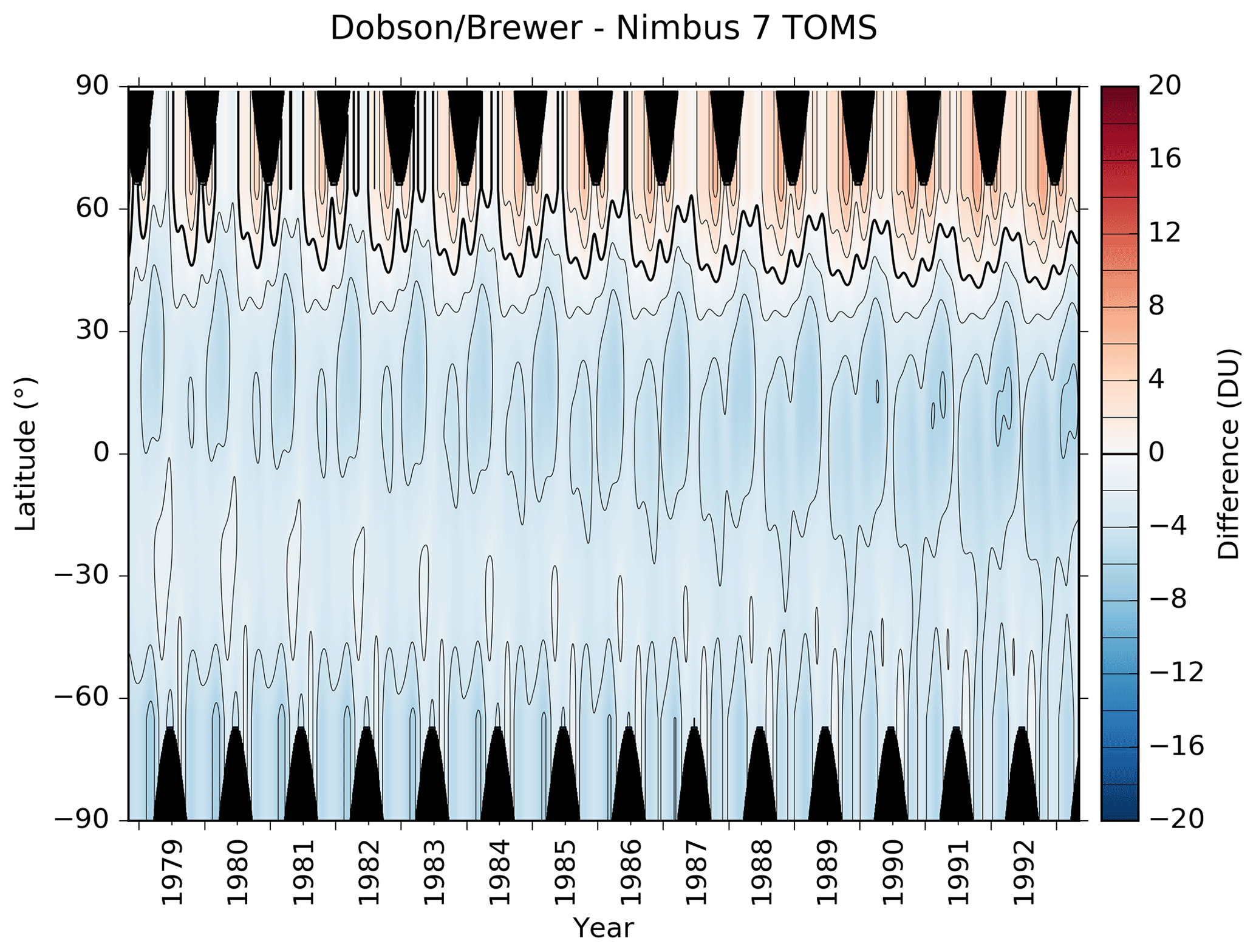
Figure 2The results obtained by fitting Eq. (1) to the differences between Dobson/Brewer ground-based TCO measurements and Nimbus 7 TOMS overpass TCO measurements (ground-based minus satellite). Regions shaded in black denote the polar night where neither ground-based nor space-based measurements are possible. The thick black line denotes the zero contour. Differences are shown in Dobson units (DU; 1 DU = 2.69×10¹⁶ molecules cm−2).
The morphology of this Dobson/Brewer–Nimbus 7 TOMS difference field is similar to that shown in Fig. 2 of Bodeker et al. (2001b) but with smaller differences resulting from the use of Legendre expansions in latitude, which better accommodate hemispheric asymmetries, rather than a truncated polynomial expansion used in the earlier study. Similar Δ(t,θ) difference fields (not shown) were statistically modelled for Adeos TOMS, Earth Probe TOMS, Meteor-3 TOMS, and Aura OMI. Corrected TCO measurements for each of these data sets were calculated as follows:
where ϕ is the longitude.
The TOMS and OMI grids, corrected for their offsets and drifts against the ground-based Dobson and Brewer measurements, now form the basis to correct the other data sets listed in Table 1. Differences between 1∘ zonal means from the combined corrected TOMS/OMI data and from the remaining data sets are calculated individually for each data set. The differences are then used as input to the regression model described in Eq. (1). There could be a danger here that, in the case of biased longitudinal sampling by one satellite compared to another, the zonal means would be biased but without these differences arising from any intrinsic biases between the satellite-based measurements. Only the SBUV measurements were sparse and corrections for this potential sampling bias were derived as discussed below.
If more than one TOMS/OMI meridional transect of zonal means is available for a given day, then all available difference values are passed to the regression model. As discussed in Bodeker et al. (2005), on 22 June 2003, a tape recorder failure on the European Remote-Sensing 2 (ERS-2) satellite resulted in only a small portion of the Northern Hemisphere being sampled by the GOME instrument thereafter. To account for possible discontinuities in the difference field introduced by this anomaly, an additional basis function was included in the regression model for the TOMS/OMI – GOME differences, set to 0 prior to 22 June 2003 and to 1 thereafter. The resultant fit to the differences between zonal means of TOMS/OMI and GOME is shown in Fig. 3.

Figure 3The results obtained by fitting Eq. (1) to the differences between corrected TOMS/OMI TCO zonal means and GOME TCO zonal means. An additional basis function is included to account for the 22 June 2003 anomaly. Regions shaded in black denote the polar night where space-based measurements in the UV–visible part of the spectrum are not possible. The thick black line denotes the zero contour.
The effects of the 22 June 2003 anomaly are clear in Fig. 3, with higher and more variable differences after 22 June 2003 than before. Statistically modelled difference fields, similar to that shown in Fig. 3, were generated for all non-TOMS/OMI data sets and extended, as required, to span the temporal coverage of each of those data sets to permit correction of the full data set. Because the combined TOMS/OMI record spans nearly the whole period (November 1978 to December 2016), extension into periods where TOMS/OMI data are not available is uncommon.
In addition to deriving the corrections for each data set listed in Table 1, the uncertainties on each of these corrections were also calculated since they contribute to the uncertainties of the respective data set as discussed in Sect. 5. The overall uncertainties on each of the source data sets are used to create an uncertainty-weighted mean of all source data sets to produce the final TCO databases (see Sect. 6).
One attribute of this version of the NIWA-BS TCO database that differentiates it from previous versions is the provision of uncertainty estimates on each TCO value in the database. This development has been driven, in large part, by the requirements for a climate data record as stipulated in GCOS-143 (2010). Table 2 gives an overview of the literature on which we have based the uncertainty estimates of our source data sets. For the NPP-OMPS instrument, the uncertainty on each TCO measurement comprises both a static component (in DU), and a component that scales with the TCO; i.e. it is a percentage of the TCO. The relevant values (1.12 DU for the static component and 0.64 % for the component that scales with TCO) were derived from a linear fit to the data listed in Table 7.3-7 of Godin (2014).
Basher and Bojkov (1995)Fiolotev et al. (2005)Krueger et al. (1998)McPeters et al. (1998)Herman et al. (1996)McPeters et al. (1996)Bhartia (2002)Godin (2014)Table 2Typical uncertainties on the source data sets as reported in the references provided and as used in the construction of the TCO databases. Note that the uncertainty on any particular measurement may differ from the typical values quoted in this table.

The random uncertainties on the raw values listed in Table 2 are propagated through the analysis to result in an uncertainty estimate on the final product. When regression modelling the difference field between the ground-based Dobson/Brewer measurements and the TOMS/OMI overpass TCO measurements, the uncertainties passed to the regression model (Eq. 1) are
where σDB is the measurement uncertainty on the Dobson/Brewer measurements (1 %) and σTOMS/OMI ovp is the measurement uncertainty on the TOMS/OMI overpass measurements.
The uncertainty on the modelled difference field is calculated using a Monte Carlo approach, whereby the uncertainties on each difference pair are used to generate new estimates of the differences which then constitute a new data set of differences to which the statistical model is fitted. The process is repeated 100 times. The mean and standard deviation of the 100 resultant model fits provide the final difference field and its uncertainty (σΔ). The uncertainties on the corrected TOMS/OMI values, calculated using Eq. (3), are then given by
A similar procedure is used to propagate uncertainties in the corrections of the other satellite data sets against the corrected TOMS/OMI data sets. Recall that these corrections are based on comparisons of zonal means. To estimate the uncertainties on the zonal means, rather than taking the weighted mean of the single measurements, the unweighted arithmetic mean is calculated so that every measurement has the same weight. The zonal mean (ZM) and its uncertainty (σZM) are then given by
where N is the number of measurements in the zone, xi indicates the measurements, and σi indicates the uncertainties on the measurements. The uncertainty on the zonal mean also needs to account for the effects of any undersampling. If the zonal profile of TCO is highly structured, perhaps as a result of planetary-scale waves, then, if a particular space-based instrument does not fully capture that structure, the uncertainty on the zonal mean will be higher than would have been the case otherwise. This is primarily a concern for the sparse sampling by the SBUV instruments used to create the combined database. For the SBUV data sets, in addition to the zonal mean uncertainty calculated using Eq. (6), the potential uncertainty resulting from the sparse sampling was also accounted for. To estimate this additional uncertainty in the zonal means calculated using SBUV measurements, an algorithm was developed to compare the zonal mean of a well-sampled zonal TCO profile with the zonal mean calculated using the same zonal profile but sampled at the SBUV measurement locations. The high-spatial-resolution (0.25∘) OMI data set was used for this purpose. To estimate the potential zonal mean uncertainty for each day of the year resulting from the SBUV undersampling, grids of high-spatial-resolution data from OMI were considered for 10 years (2004 to 2013) and for 10 d before and after the day of interest, totalling 21 d. This gives a sample data set of 210 data grids. For each SBUV data set available on that calendar day, and for each latitude, two zonal means are calculated, namely (1) the true zonal mean (ZMtrue) calculated from the 1440 values comprising the zonal TCO profile at 0.25∘ resolution, and (2) the subsampled zonal mean (ZMsub) calculated using only those OMI data at the locations of the SBUV measurements. For each latitude, 210 (from the 21 d window of 10 years of OMI data used) difference pairs of ZMtrue−ZMsub can be calculated. If the SBUV sampling of the zonal mean was unbiased, all 210 values would be 0.0. The mean and standard deviation of these 210 values are then calculated, and the standard deviation is used as an estimate of the SBUV subsampling uncertainty (σsubsample) which is specific to a particular SBUV instrument and depends on the year and latitude. An example of one such subsampling uncertainty field for the NOAA 19 SBUV instrument is shown in Fig. 4.
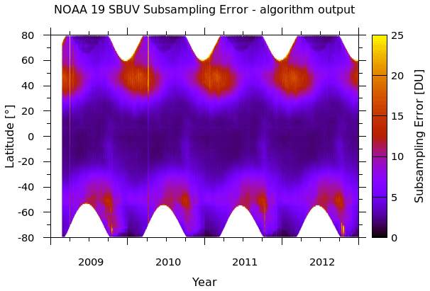
Figure 4The additional uncertainty introduced to the SBUV zonal means as a result of undersampling the zonal TCO profile. Regions shaded in white denote the polar night where space-based measurements in the UV–visible part of the spectrum are not possible.
The subsampling uncertainty maximizes during periods when the zonal profile shows more complex structure, i.e. typically in winter and spring when midlatitude planetary wave activity maximizes. The subsampling uncertainty on the zonal means is added to the zonal mean uncertainty calculated using Eq. (6) as
To construct a single TCO field for each day, a weighted mean of all available corrected measurements in each grid cell is calculated. A grid of 1.25∘ longitude by 1.0∘ latitude was selected for the final product. The weights applied to the individual available TCO measurements are derived from the measurement uncertainties on each available measurement, namely
where i and j are indices over latitude and longitude, k is an index over the measurements from different satellites in that cell, and the weights () are calculated as , where σ is the measurement uncertainty incorporating any additional uncertainty introduced by corrections made to the original data. Unlike previous versions of this TCO database, the daily combined TCO fields are accompanied by fields of uncertainties and fields detailing the number of values that were averaged to produce the single combined value. An example of these three fields for one selected day is given in Fig. 5.
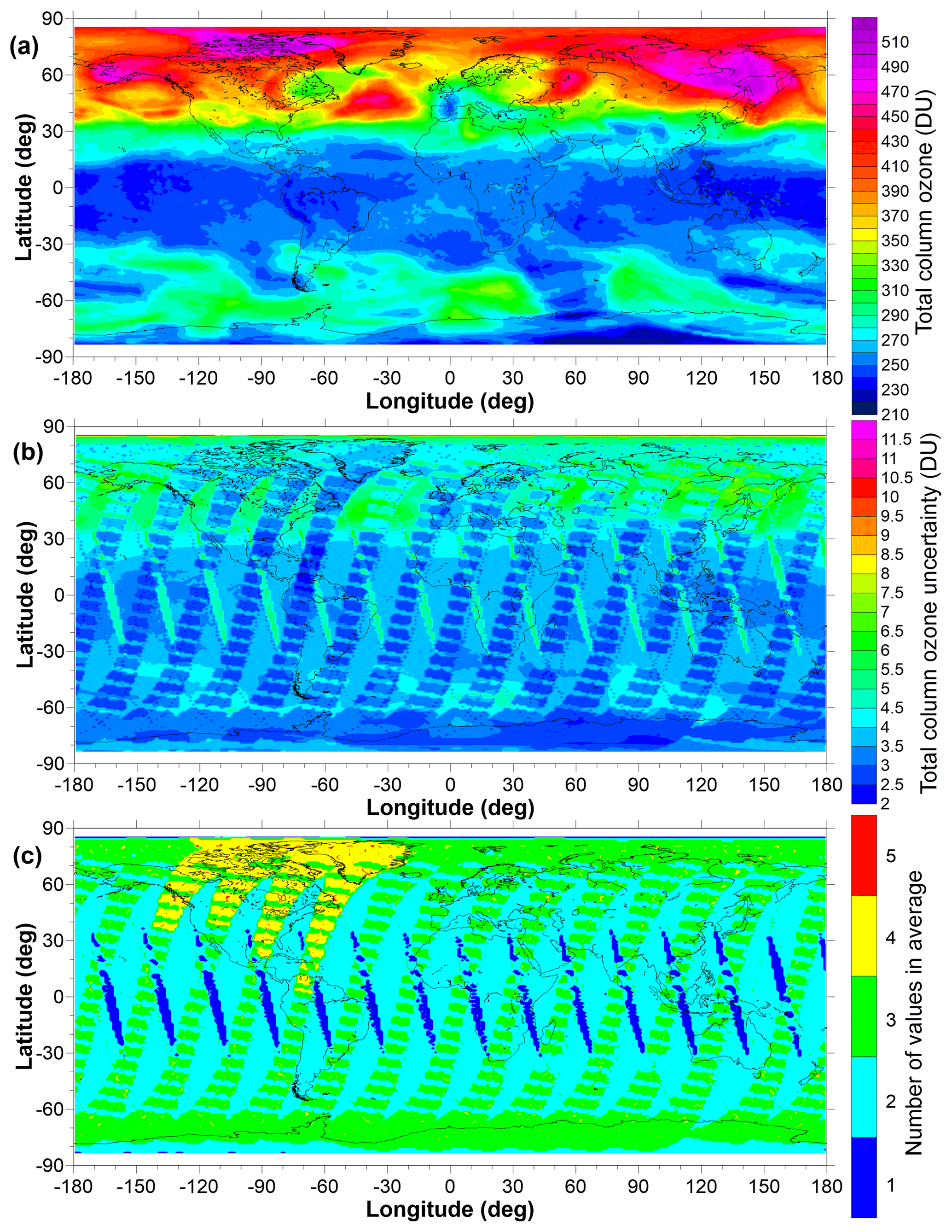
Figure 5Example fields for 21 March 2005: (a) the TCO field, (b) the uncertainties on each value plotted in panel (a), and (c) the number of values averaged to create the means plotted in panel (a). Regions shaded in white denote the polar night where space-based measurements in the UV–visible part of the spectrum are not possible.
As expected, Fig. 5 shows that the uncertainty on TCO values decreases with an increasing number of source data sets. The regions of elevated uncertainty, sloping from north-west to south-east across the Equator, arise from having only the OMI TCO values available to build the mean. Cyan regions in Fig. 5c show where additional Earth Probe TOMS data contribute (with a resultant reduction in the uncertainty) and regions in green where SCIAMACHY additionally contributes data, reducing the uncertainties in the resultant mean to less than 3 DU.
This new NIWA-BS TCO database has been validated through comparisons with the WOUDC database and four additional independent TCO databases listed in Table 3. To account for different spatial resolutions, the NIWA-BS database was regridded to match the spatial resolution of each validation database. The differences reported in this section were calculated by subtracting the validation values from the NIWA-BS values such that positive differences represent elevated ozone values in the NIWA-BS database compared to the validation databases. Figure 6 shows the globally averaged area-weighted differences between the NIWA-BS database and the validation databases over the full time period.
McPeters et al. (2013); Frith et al. (2014)Wild et al. (2012); McPeters et al. (2013)Weber et al. (2013)Lerot et al. (2014)Table 3Sources and details of the independent data sets used to validate the NIWA-BS total column ozone database.
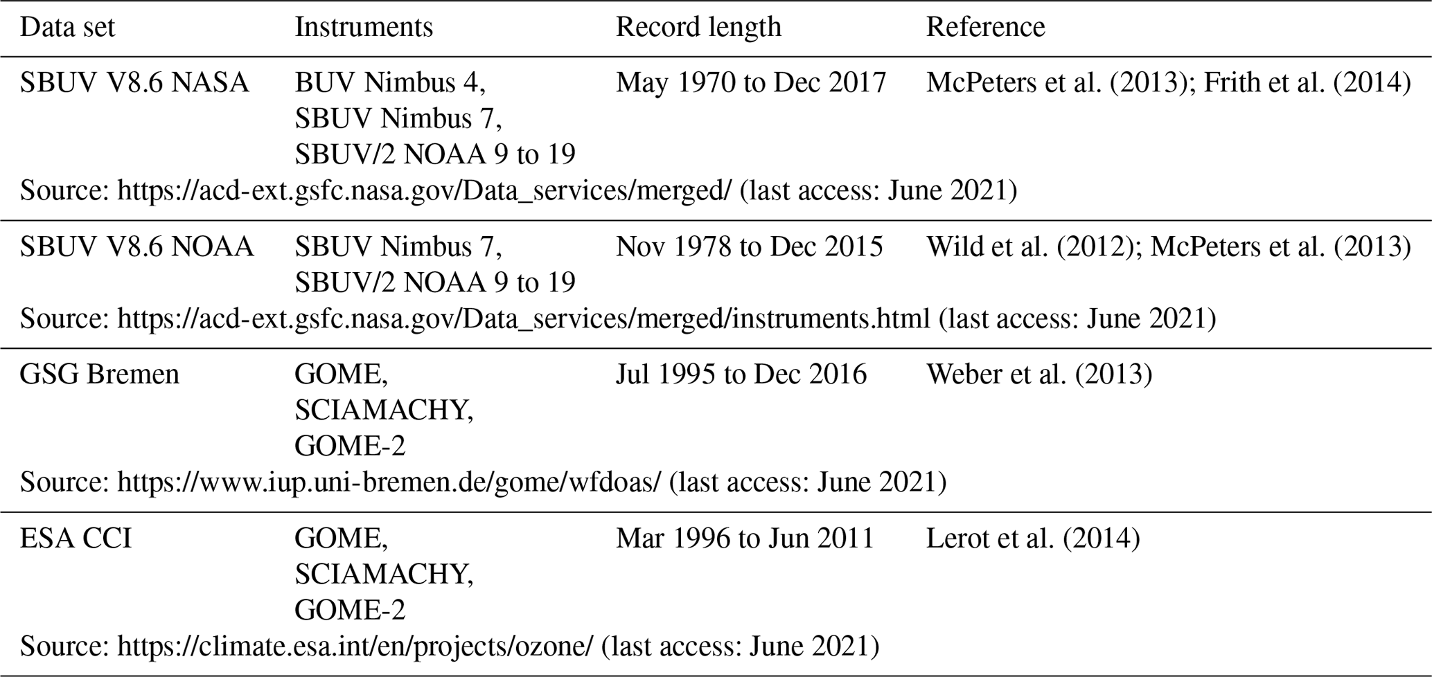

Figure 6Area-weighted global mean monthly mean differences in TCO between the NIWA-BS database and the validation databases detailed in Table 3. The topmost panel shows the differences between the NIWA-BS database and the ground-based TCO database obtained from the WOUDC. The remaining four panels show differences against databases derived from space-based measurements. The statistics in the top right corner of each panel show the mean difference and standard deviation.
The NIWA-BS database displays a small negative bias ( DU) against the global mean monthly means calculated from the Dobson and Brewer measurements obtained from the WOUDC. A slightly larger negative bias ( DU) is seen in comparison with the SBUV V8.6 NASA time series. The bias against the SBUV V8.6 data set produced by NOAA is slightly more negative but not statistically significantly different from zero ( DU). The comparison against the GSG Bremen database suggests that the NIWA-BS time series exhibits a small anomalous downward trend starting around 2002, which is also reflected in the WOUDC comparison and in the ESA CCI comparison.
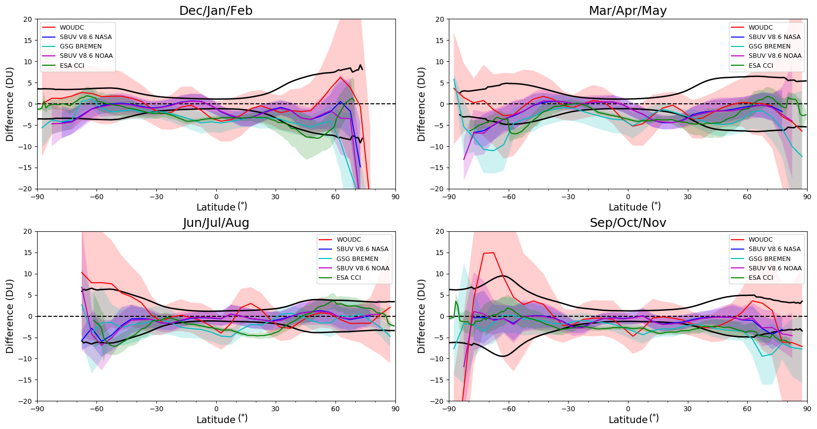
Figure 7TCO differences (NIWA-BS TCO minus validation database) as a function of latitude plotted as seasonal means over the entire period of data available. The 1σ uncertainty range in the NIWA-BS TCO is shown in black and the standard deviation on the differences between NIWA-BS TCO and each validation database is shown by the shading.
Seasonal mean differences between the NIWA-BS database and the five validation databases, as a function of latitude, are shown in Fig. 7. In general, the differences between the NIWA-BS TCO database and the validation databases are smaller than the uncertainties in the NIWA-BS database. This is not the case, however, in the high northern latitudes in winter where the NIWA-BS database shows statistically significantly smaller ozone values compared to the validation data sets. This results from larger differences in satellite measurements and ground-based measurements being inferred close to the region of permanent polar darkness where both satellite and ground-based measurements are scarce; i.e. there were only 548 Dobson/Brewer–satellite difference pairs in the winter (DJF) Arctic (poleward of 60∘ N) on which to base the correction.
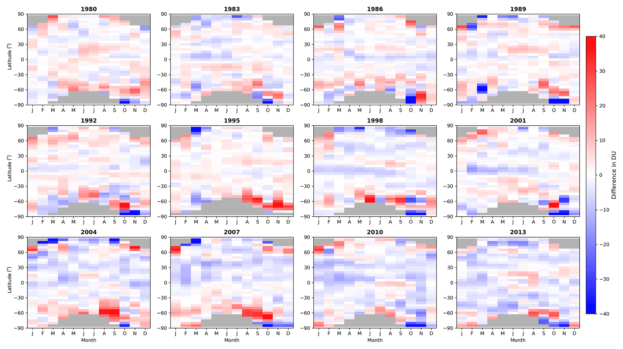
Figure 8Monthly mean differences between NIWA-BS TCO and the WOUDC database for 12 selected years.
A more in-depth comparison of the NIWA-BS database and the WOUDC database is presented in Fig. 8, where monthly mean zonal means (in 5∘ latitude zones) are differenced (NIWA-BS minus WOUDC). Over their full period of overlap, the mean difference between the data sets is −0.26 DU, with 95 % of the differences falling between −11.38 and 13.21 DU. Differences between the data sets are larger at higher latitudes. A consistent feature of the NIWA-BS TCO database across most years is an overestimation in TCO equatorward of the Antarctic and an underestimation of TCO close to the South Pole with respect to WOUDC.
Differences between monthly mean 5∘ zonal means from the NIWA-BS database and NASA SBUV merged ozone database version 8.6 are shown in Fig. 9.
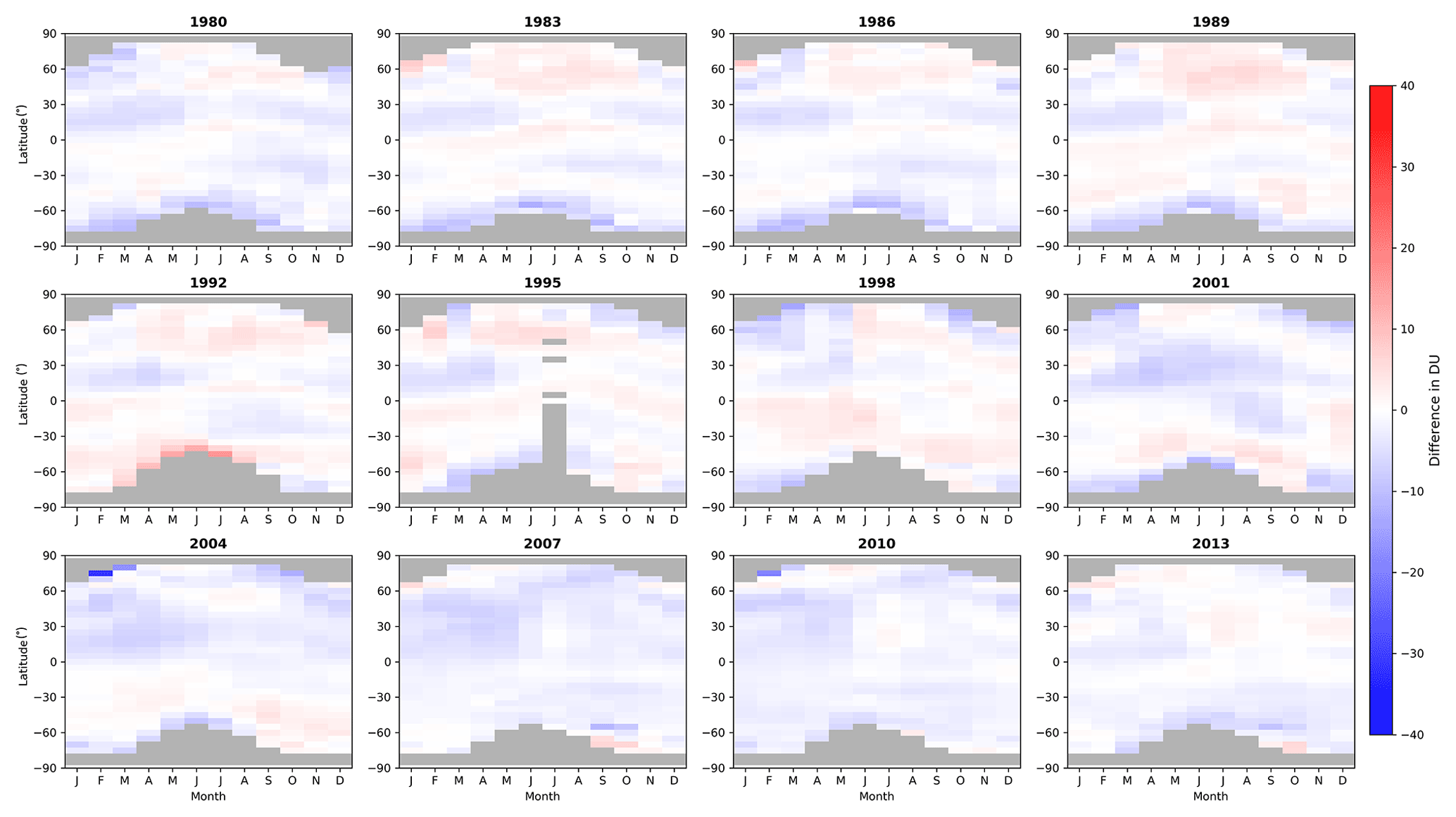
Figure 9Differences between monthly mean zonal means calculated from the NIWA-BS TCO database and the NASA SBUV V8.6 database (NIWA-BS minus SBUV) for 12 selected years.
The mean difference in TCO across the full overlap period is −1.21 DU, with 95 % of the differences in the range −5.96 to 2.95 DU. The differences are smaller in magnitude than those shown in Fig. 8 and show smaller year-to-year variability, perhaps as a result of the more dense spatiotemporal sampling by the SBUV instruments compared to the ground-based instruments. Features common across most years are an underestimation of TCO in the northern subtropics during the first half of each year and underestimations just equatorward of the polar night in the Southern Hemisphere.
As the NOAA SBUV database is available at daily resolution as for the NIWA-BS TCO database, daily differences between zonal means from these two databases are calculated and shown in Fig. 10.
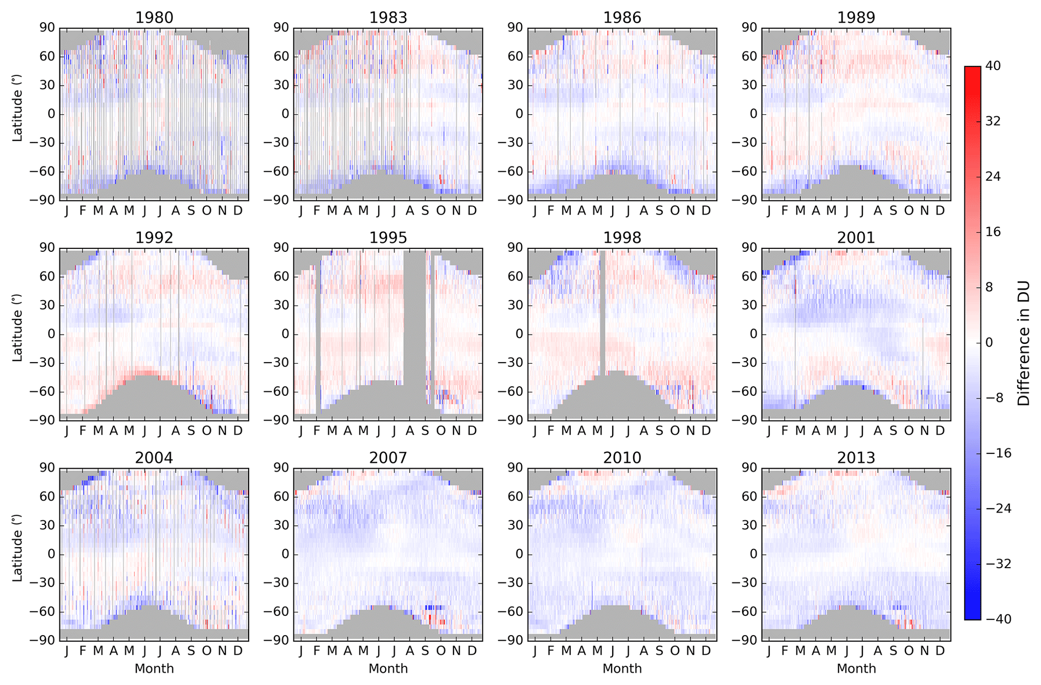
Figure 10Daily differences between 5∘ zonal means calculated from the NIWA-BS TCO database and the NOAA SBUV V8.6 database for the same years as in Fig. 9.
Over their full overlap period, the average difference is −1.44 DU, with 95 % of the differences between −8.66 and 5.35 DU. Similar to the NASA SBUV comparisons, there appears to be a small underestimation in TCO over the northern subtropics in the first half of many years.
Differences between monthly mean 5∘ zonal mean TCO from the NIWA-BS database and the GSG Bremen TCO data set which combined GOME, SCIAMACHY, and GOME-2 data are shown in Fig. 11.

Figure 11Differences between monthly mean 5∘ zonal mean TCO calculated from the NIWA-BS and GSG Bremen databases for 12 selected years (NIWA-BS minus GSG).
There appears to be a consistent underestimation of TCO in the NIWA-BS database equatorward of the polar night from January to March in most years with respect to GSG Bremen. The mean difference between the databases is −3.14 DU, with 95 % of the differences lying between −9.79 and 2.81 DU.
Validation data from the ESA Climate Change Initiative (CCI) level 3 TCO data set are available as monthly mean maps, and differences between these monthly mean maps and NIWA-BS TCO are shown in Fig. 12.
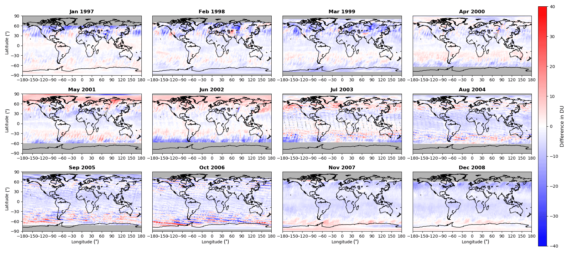
Figure 12Differences between monthly mean TCO fields calculated from the NIWA-BS database and those available from the ESA CCI database for 12 selected months/years.
While there is significant spatial structure in some of the monthly difference fields, there is little structure that is consistent across multiple years. The mean difference is −2.36 DU, with 95 % of the differences lying between −10.63 and 6.34 DU.
Monthly mean TCO fields at 1.25∘ longitude and 1∘ latitude resolution (the same resolution as the daily fields) have been calculated, together with their uncertainties. The algorithm was used to calculate the mean and its uncertainty from N measurements (xi, ). The uncertainty on the mean is calculated in such a way that it depends on both the uncertainties on the measurements (σi) and on the variance in the measurements. First, a revised uncertainty for each datum is calculated to reflect the true confidence we have on each measurement as an estimator of the mean:
where xi,exp is the “expectation” value which is taken to be the unweighted mean of the available measurements. The mean is then calculated as
where and the uncertainty is calculated as
where and NF is the degrees of freedom. In this case, NF was taken to be N−1 to account, in part, for auto-correlation in the daily time series used to calculate the monthly and annual means. The monthly mean and annual mean TCO fields are provided as a component of the version 3.4 database.
For some applications, there is a need for gap-free TCO fields, e.g. TCO fields for validating chemistry-climate models which generate TCO fields over the entire globe for each day of the year. To create a filled TCO database for a target day, the following steps are performed, each of which is detailed in subsections below.
-
A conservatively partially filled field is created (hereafter referred to as Field 1).
-
A ML method is used to create a best estimate of the completely filled TCO field for the target day (hereafter referred to as Field 2).
-
The original unfilled TCO field, Field 1, and Field 2 are then “blended” (using an algorithm described below) to generate the final filled field.
The result is a TCO field that replicates the original data where they are available and, where no data are available, transitions preferentially into the conservatively filled field (Field 1). Where the conservatively filled field has missing data, we transition into the ML-filled field (Field 2). Each “transition” is achieved by way of the blending process described below.
9.1 The conservatively filled field – Field 1
First, a spatial nearest-neighbour interpolation is used to fill as many missing values as possible. This is done by searching for cells with null TCO values that are neighboured, either to the north and south, or to the east and west, by non-null values. If such a non-null pair is found, that pair of TCO values, together with their uncertainties, is used to estimate the interstitial value which is taken as the mean of the two neighbouring values. Preference is given to zonal nearest neighbours. The uncertainty on the interpolated values is calculated by adding in quadrature the uncertainties on the neighbouring values.
After doing the spatial nearest-neighbour interpolation, cases are sought where, for a cell containing a null value on day N, there are non-null values in the same cell on day N−1 and day N+1. Temporal nearest-neighbour interpolation between the previous and following day is done in the same way as described for the spatial nearest-neighbour interpolation.
Following the spatial–temporal nearest-neighbour interpolation, a more extensive longitudinal interpolation finds two non-null values at the same latitude that are separated by two or more null values with the constraint that the non-null values cannot be separated by more than 30∘ in longitude. Linear interpolation between the two non-null values, including an estimate of the uncertainties, is used to determine the interstitial values and their uncertainties. The spatial–temporal nearest-neighbour interpolation, and the longitudinal interpolation, are repeated until no additional values are inserted into the grid. The result is a conservatively interpolated TCO field, still containing missing values, together with its original uncertainty field and traceable uncertainties on the newly interpolated values. A plot of the original TCO field, the conservatively filled field, and the uncertainties on the conservatively filled field for day 3 of 1980 are shown in Fig. 13.
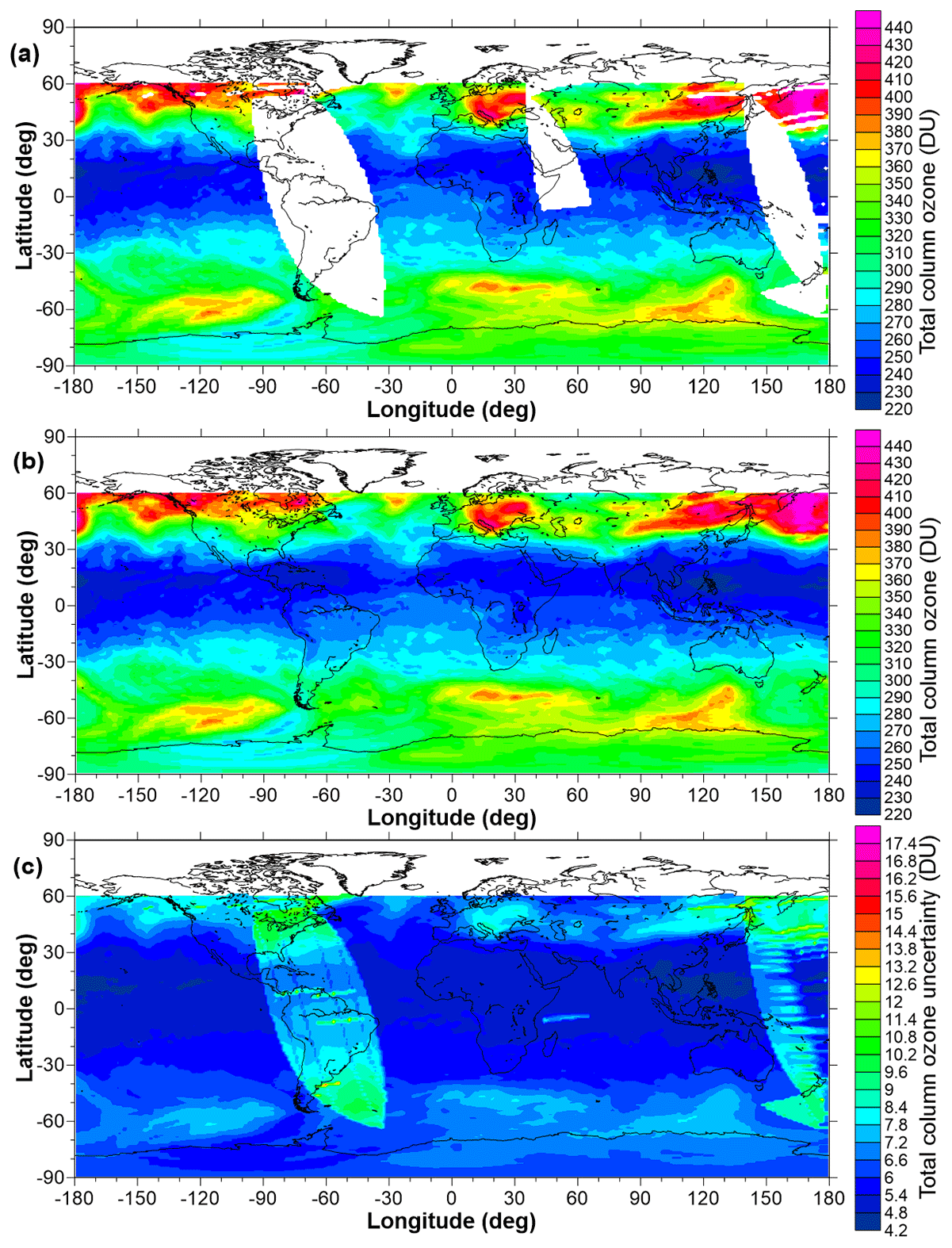
Figure 13(a) The original unfilled TCO field on 3 January 1980, (b) the conservatively filled TCO field on the same day, and (c) the uncertainties on the conservatively filled field. White regions show where data are missing.
The structure in the uncertainty field results from the propagation of uncertainties when calculating the conservatively filled field – larger uncertainties result when interpolated values are spatially far from available measurements.
9.2 The machine-learning-estimated field – Field 2
To create a completely filled TCO field for each day, a regression model, including an offset basis function, a tropopause height basis function, and a potential vorticity at 550 K basis function, is trained on a “window” of data around the target date. The trained regression model is used to generate a filled TCO field on the target date.
The regression model is of the form
where i,j subscripts denote indices over latitude (θ) and longitude (ϕ), TH and PV550 are 6-hourly tropopause height fields and 500 K potential vorticity fields, respectively, obtained from NCEP CFSR (National Centers for Environmental Prediction) CFSR (Climate Forecast System Reanalysis) reanalyses prior to 31 December 2010, and from NCEPCFSv2 reanalyses thereafter (Saha et al., 2010). α, β, and γ are fit coefficients and Ri,j are the residuals that remain due to variance that cannot be explained by the regression model.
As denoted in Eq. (12), the three fit coefficients depend on latitude and longitude. That dependence is captured by expanding the fit coefficients in spherical harmonics in a similar way as was done in Eq. (2), i.e.
where
-
θ is the co-latitude,
-
ϕ is the longitude,
-
N is a regression model parameter,
-
where the exact limit for l′ is also a regression model parameter,
-
indicates the fit coefficients, and
-
is the spherical harmonic function of degree l and order m.
The can be expressed as
For the purposes of fitting Eq. (14) to the TCO fields, the normalization constants () can be ignored as they are taken up into the fit coefficients. When fitting Eq. (12), the initial N value for α is set as 10 and for β and γ as 2. The maximum allowed N value for α is 10 and for β and γ is 5. The initial l′ value for α was set at 5 (with a maximum allowed value of 5) and for β and γ as 2 (with maximum allowed values of 5). These initial values and limits on the spherical harmonics expansions were selected based on careful consideration of the scales of spatial structures in TCO fields, and on how the dependence of TCO on TH and PV550K varies spatially. The training of the algorithm happens “around” the target date as fields on neighbouring dates and years are used to establish the dependence of TCO on TH and PV550K. A search ellipse, initially extending 3 d on either side of the target date, and 1 year on either side of the target date, is defined to select TCO fields for the training where the ellipse is iteratively expanded until there are 20 TCO fields available for the training. The extension to neighbouring years is done because, in some cases, there are missing TCO fields in the current year such that a reliable fit of Eq. (12) cannot be performed. Within this search ellipse, the dependence of TCO on TH and PV550K at a similar time of the year is expected to hold.
From these 20 TCO fields, to avoid excessive computational expense, only up to 20 000 data points are passed to the regression model by sampling every lth value from all data available for training such that the total number of values passed is less than or equal to 20 000. The latitude and longitude of each ozone value is also passed to the regression model so that the associated TH and PV550K values can be extracted. The times associated with the TCO fields are assumed to be local noon times (since most of the satellites making the underlying measurements were Sun-synchronous satellites with an Equator-crossing time close to solar noon). Therefore, the actual UTC time varies across the TCO field. The TH and PV550K values are linearly interpolated to those exact UTC times.
Various “versions” of the regression model are tested; i.e. different basis functions are excluded/included; the offset (α) basis function is always included. In addition to switching different basis functions on/off, different values for N and l′ are tested (perturbing these by ±1 around their start value) but ensuring that the maximum allowed zonal and meridional expansions are not exceeded (see above). This results in many different possible constructs of the regression model. If any model, when evaluated over every latitude and longitude, results in a TCO value more than 10 % above the maximum measured TCO value passed to the regression model, or below 10 % less than the minimum value passed to the regression model, it is discarded to eliminate statistical models that significantly overfit the TCO field. In addition to having a model with an excess of fit coefficients, overfitting can also occur when anomalous values in the TH or PV550 fields result in excessively high or low TCO values being generated. This is why models that exclude/include these two basis functions are also tested. For all models that pass this initial test, a Bayesian information criterion (BIC; Liddle, 2007) score is calculated as
where M is the number of data passed to the regression model, R2 is a modified sum of the squares of the residuals, and NC is the total number of coefficients in the fit. R2 is modified to provide a strong disincentive for models generating values outside the range of measurements, i.e. where model values are below the minimum or above the maximum measurement passed to the regression model, the residual is inflated exponentially to impose an additional cost on the model for generating values outside of the range of the data.
Typically, for each daily TCO field, several hundred fits of the regression model are performed to find the optimal model construct (minimum BIC). This optimal model is then used to generate the statistically modelled TCO field. The database of different regression models is also used to calculate the structural uncertainties that result from different possible choices of spherical harmonic expansions. The uncertainties that result from uncertainties on the regression model fit coefficients are also calculated. These two sources of uncertainty are then added in quadrature. The structural uncertainty statistics are calculated using only those regression modelled fields (out of the several hundred) that have the same sequence of basis functions switched on and off compared to the best fit. Examples of the unfilled TCO fields, the ML-modelled TCO fields, and the uncertainty on the modelled TCO fields for days 304 and 305 of 1978 are shown in Fig. 14.
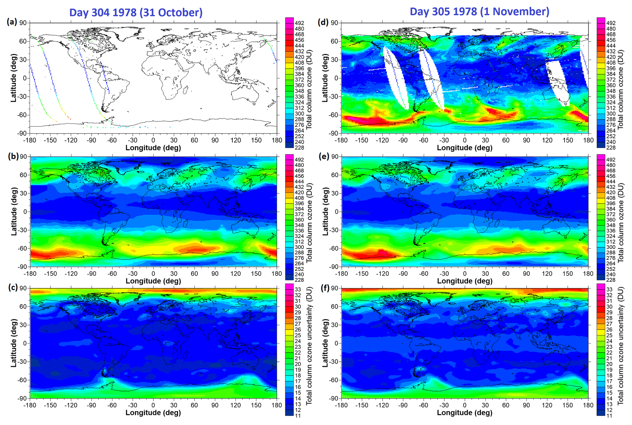
Figure 14(a, d) The original unfilled TCO fields on 31 October and 1 November 1978, respectively; (b, e) the machine-learning-modelled fields; (c, f) the uncertainties associated with the machine-learning-modelled fields. On 31 October, the optimal fit was obtained by expanding the offset basis function in spherical harmonics of degree 10 and order 5, expanding the tropopause height basis function in spherical harmonics of degree 4 and order 3, and the PV at 550 K basis function in spherical harmonics of degree 5 and order 3. For 1 November, these expansions were (10,5) for the offset basis function (4,3) for the TH basis function and (5,4) for the PV550K basis function.
9.3 An algorithm for blending a primary and secondary TCO field
This section describes an algorithm to “blend” some primary TCO field (hereafter Field A) with some secondary field (hereafter Field B) to create a single blended field (hereafter Field C), where the Field A values are preserved while smoothly transitioning to the Field B values. This algorithm is used below to combine the original TCO field and Field 1, and/or to combine Field 1 and Field 2, and/or to combine the original TCO field and Field 2; see Sect. 9.4.
If there is a null value in a cell in Field A and a non-null value in the same cell in Field B, then a proxy value for Field A is found and combined with the value from Field B as follows:
where C is the blended value, W is a weight calculated as detailed below, Aproxy is a proxy value for the missing value in Field A determined as detailed below, and Bvalue is the non-null value from Field B. To derive an Aproxy value, a box of size 41×41 cells is centred on the missing value and divided into six sectors each subtending an angle of 60∘. Each sector is scanned for non-null values in Field A, and a weighted mean of those six values is calculated these weights:
where D is the distance to the nearest non-null value in that sector measured in metres. The weight is set to zero when D is greater than 1000 km. Aproxy is then set to the weighted mean of the non-null values across all six sectors.
In calculating the blended value using Eq. (16), the weight (W) is calculated using the distance to the nearest non-null value across all six search sectors in Eq. (17). If no Aproxy value can be found, then W in Eq. (16) is set to zero. Standard error propagation rules are used to determine an uncertainty on the blended value. This process results in using values from Field A where they are available which then blend into values from Field B when they are not available.
9.4 Blending the original unfilled TCO field, Field 1, and Field 2 to construct the final filled field
For each day, the original TCO field, the conservatively filled field (Field 1), and the ML-modelled field (Field 2) are merged in such a way that the original values are preserved where they are available. Where they are not available, the filled values relax to the conservatively filled field where they are available. Where conservatively filled values are also not available, the filled values relax to the ML-modelled field.
The ML-modelled fields, because they are modelled on PV550K and TH (which themselves can contain anomalous values), can occasionally display physically unrealistic spatial or temporal structures so, for any given day, to obtain a smoother ML-filled field, a weighting of the five daily ML-filled fields, centred on the day of interest, is calculated.
For the final blended data product, several possibilities exist for any given day, i.e.
-
None of the three fields are available: in this case, no final filled field is generated.
-
Only the ML-modelled field is available: in this case, the ML-modelled field (possibly spatially smoothed) and its associated uncertainties become the final filled field for the target day.
-
Only the conservatively filled field and the ML-modelled fields are available: in this case, the conservatively filled field (Field 1) and the ML-modelled field (Field 2) are blended to create the final filled field.
-
All three fields are available: in this case, the conservatively filled field and the ML-modelled field are blended to create an intermediate field. The original TCO field and the intermediate field are then blended to create the final filled TCO field and its uncertainty.
An example of the original field for TCO on 31 October 1978, the conservatively filled field, final field obtained from the blending process, and the uncertainty on the final filled field are shown in Fig. 15 (the ML-modelled field for that day can be seen in Fig. 14).
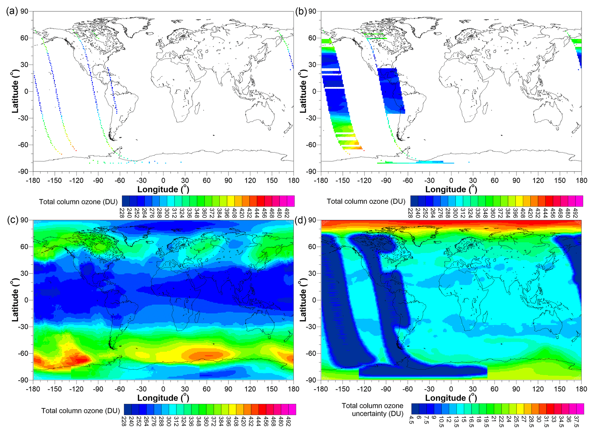
Figure 15(a) The original unfilled TCO field on 31 October 1978, (b) the conservatively filled field, (c) the final filled field, and (d) the uncertainties on the final filled field.
To prove the utility of the NIWA-BS TCO database, trends over the whole period have been diagnosed using the following regression model, described in detail in Bodeker et al. (2013):
where is the regression modelled TCO in month m (m=1 to NY×12, where NY is the total number of years of data) and at latitude θ and longitude ϕ. The monthly mean TCO values were calculated as detailed in Eq. (10) and Eq. (11). Equation (18) is fitted independently to the monthly mean time series at each latitude and longitude. A to I are the regression model coefficients calculated using a standard least squares regression (Press et al., 1989).
The first term in the regression model (A coefficient) represents a constant offset and, when expanded in a Fourier series, represents the mean annual cycle. In addition to the offset coefficient, each fit coefficient can depend on season; e.g. TCO trends vary with season. Therefore, each coefficient is expanded in Fourier pairs, as explained in Sect. 2.2 of Bodeker and Kremser (2015). The actual number of Fourier pairs for each regression coefficient is determined by finding the optimal set of expansions across all fit coefficients that minimizes a BIC as described above. The maximum number of Fourier pairs permitted for each regression model coefficient is listed in Eq. (18). The B coefficients diagnose the trend over the full period, while the C coefficients diagnose the change in trend from 2000 onward. The year from 1999 to 2000 was prescribed as the trend transition year, as this is approximately when stratospheric chlorine and bromine loading peaked (Newman et al., 2007). We also wanted to ensure that the first trend period included data from the late 1990s as there was a greater likelihood of missing data from 1994 to 1998, and we wanted to avoid end-effect biasing in the calculation of the trends. That said, the conclusions drawn below regarding changes in trend were found to be largely insensitive to the selection of the transition year within 2 years of the selected transition year. The quasi-biennial oscillation (QBO) basis function was specified as the monthly mean 50 hPa Singapore zonal wind. The phase of the QBO varies with latitude and, to permit fitting of the phase, a second QBO basis function, mathematically orthogonalized to the first, was included in the regression model as was done in Bodeker et al. (2013).
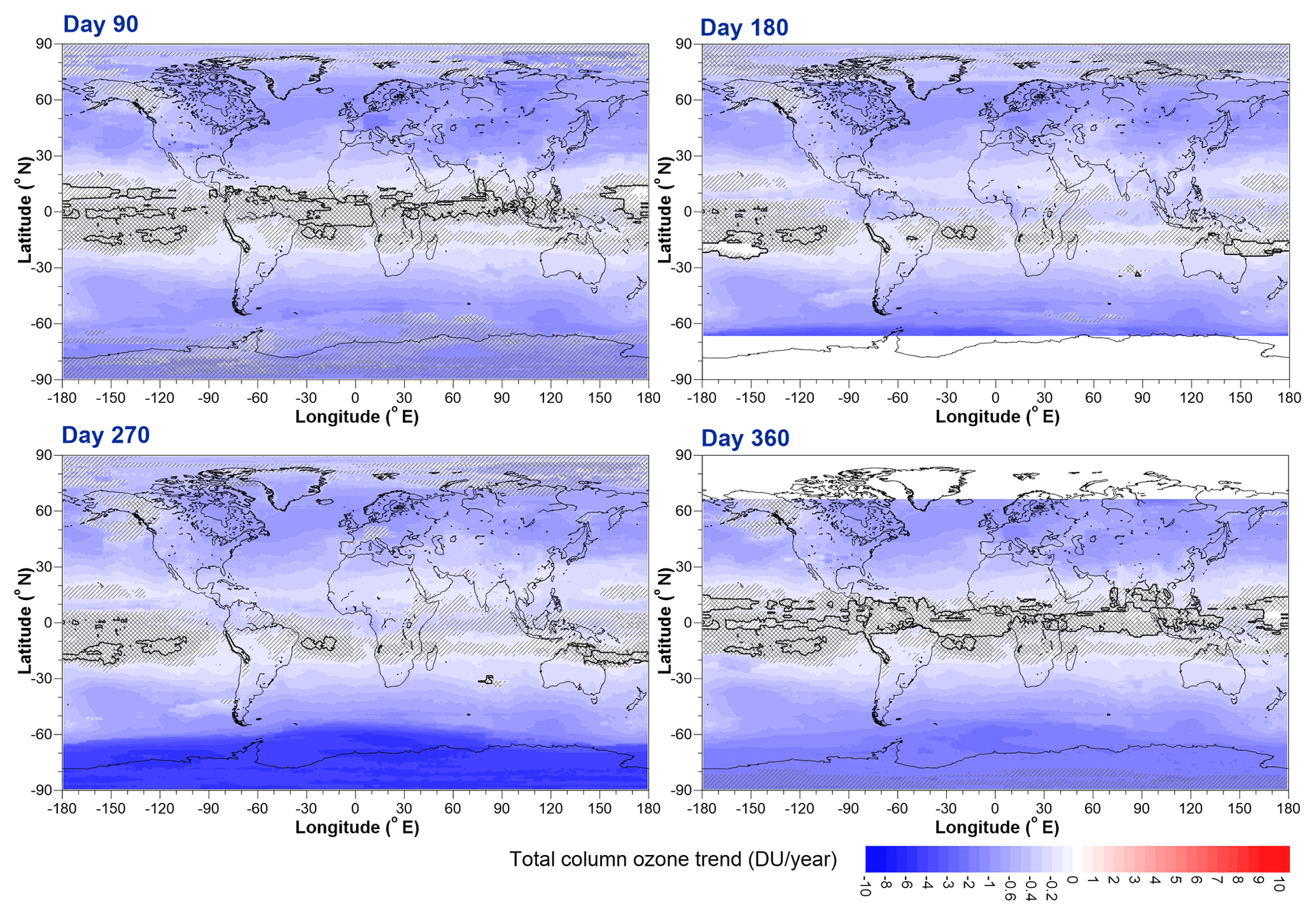
Figure 16TCO trends for the period 1979 to 2000 evaluated at (a) day 90, (b) day 180, (c) day 270, and (d) day 360. The white areas at high latitudes in panels (b) and (d) result from there being insufficient data to establish meaningful trends during the polar night periods. The solid black line shows zero trend. Double hatched regions show where trends are not statistically different from zero at the 1σ confidence level, while single hatched regions show where the trend is not statistically different from zero at the 2σ confidence level.
The El Niño–Southern Oscillation (ENSO), solar cycle, Mt. Pinatubo, and El Chichón basis functions were the same as those used in Bodeker et al. (2001b). Note that the effects of the Pinatubo and El Chichón volcanic eruptions on TCO were delayed and so temporal offsets in those basis functions, denoted by the Δm, were permitted for up to 2 years where the Δm values for each basis function were optimized as part of the same BIC optimization used to determine the optimal Fourier expansions for each regression model fit coefficient. A one-term auto-correlation model was used to account for the effects of auto-correlation in the residuals () when calculating the uncertainties on the fit coefficients.
The B coefficients, evaluated at days 90, 180, 270, and 360 through the year (noting that because these are Fourier expansions they can be evaluated at non-integral month values), are shown in Fig. 16.
The spatial and seasonal patterns of ozone trends prior to 2000 are similar to those in numerous previous studies that have shown similar trend results. The C coefficients, evaluated on the same days as the B coefficients, are shown in Fig. 17.
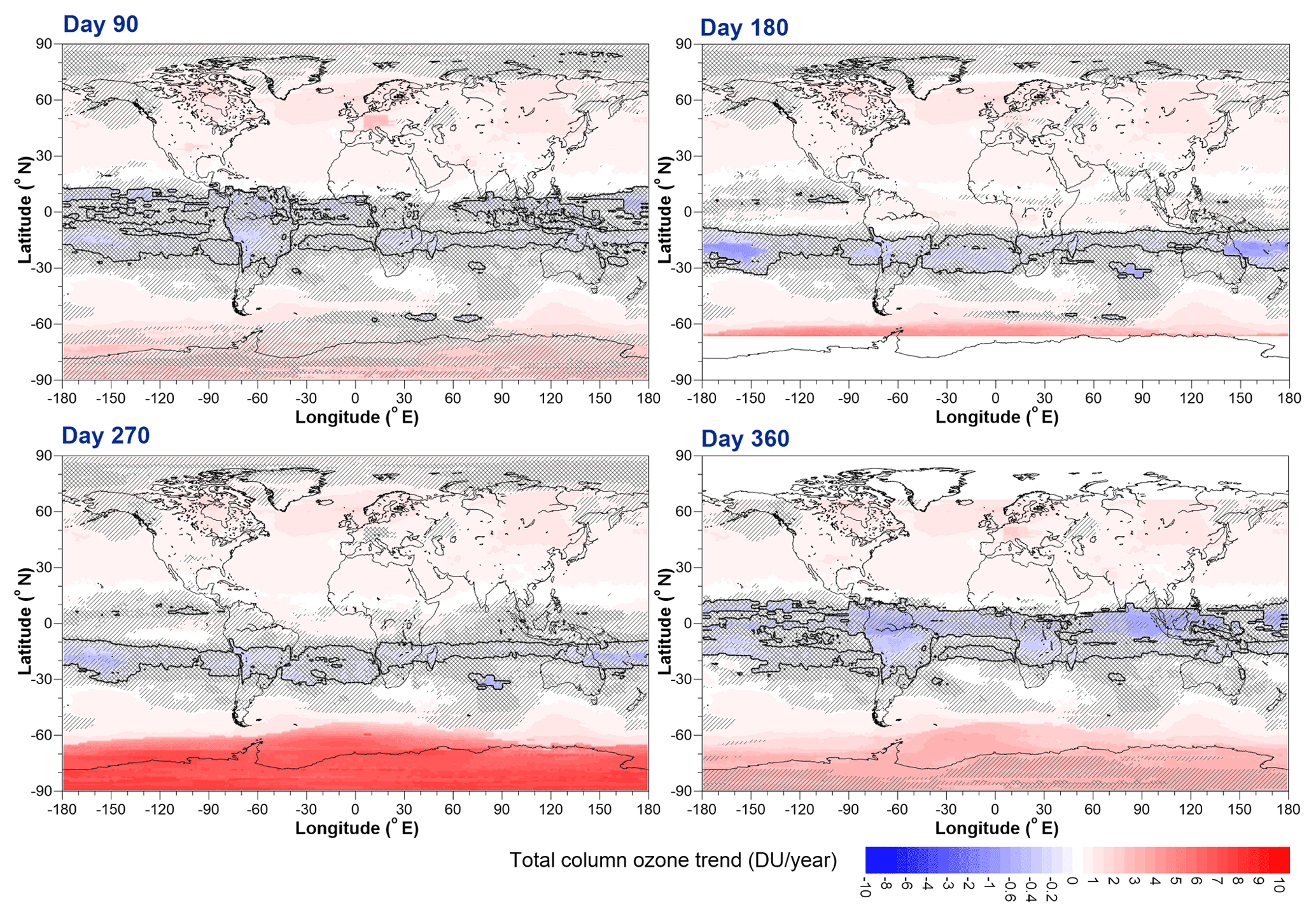
Figure 17The change in TCO trends after 2000 evaluated at (a) day 90, (b) day 180, (c) day 270, and (d) day 360. The solid black line shows zero trend. The same hatching regimen as used in Fig. 16 is used here.
Note that Fig. 17 shows the change in trend compared to the trend shown in Fig. 16; i.e. areas midway between blue (more negative trends than before 2000) and red (more positive trends than before 2000) indicate no change in trend before and after 2000. Actual trends starting from 2000 obtained by adding the trends shown in Fig. 17 to the trends shown in Fig. 16 are shown in Fig. 18.
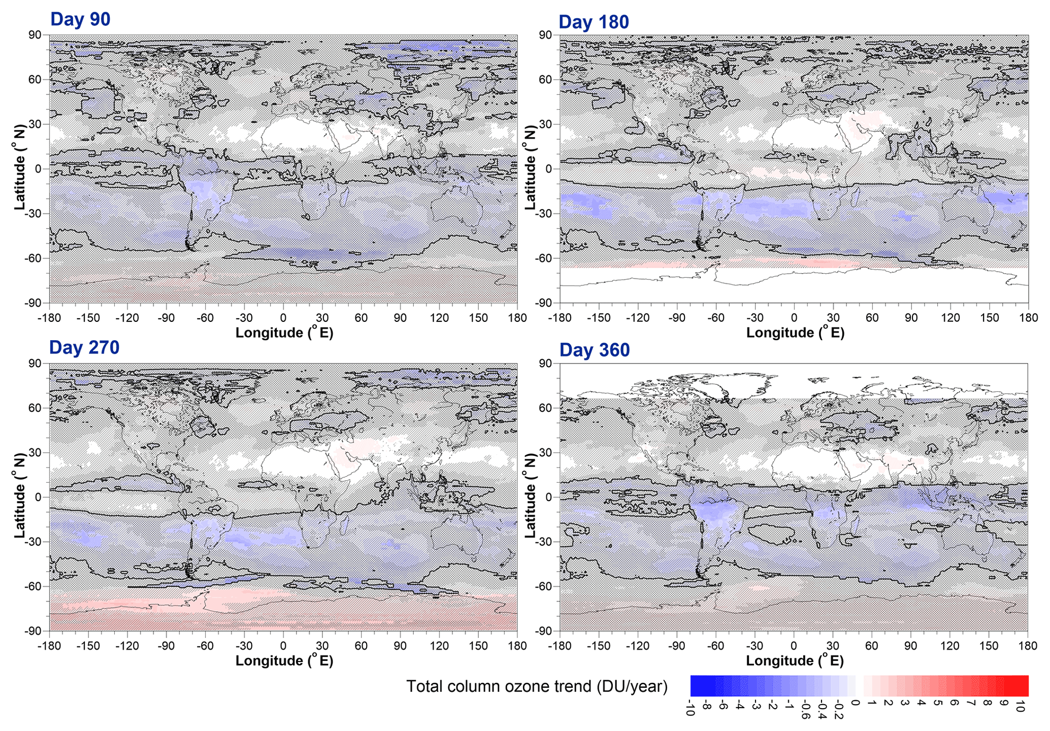
Figure 18Inferred trends in TCO after 2000 evaluated at (a) day 90, (b) day 180, (c) day 270, and (d) day 360, obtained by adding the B and C regression model fit coefficients. The solid black line shows zero trend. The same hatching regimen as used in Fig. 16 is used here.
Trends are generally seldom statistically significantly different from zero at the 2σ level. Regions of the southern middle and low latitudes continue to show declining TCO, while selected regions over Antarctica show positive TCO trends.
While, since 2000, TCO trends have largely shown a positive change compared to pre-2000 trends (particularly over Antarctica as the ozone hole recovers due to effects of declining stratospheric concentrations of ozone depleting substances), around the middle of the year a large negative change in trend in excess of −1 DU yr−1 is seen in the Southern Hemisphere subtropics. The largest of these negative anomalies occurs at 19.5∘ S, 164.375∘ W, and therefore Fig. 19 shows the July mean TCO, regression model fit for July, and the contribution of the offset and trend basis function evaluated at this location.

Figure 19The July mean total column ozone at 19.5∘ S, 164.375∘ W (blue dots) together with the regression model values (red dots) and their 1σ uncertainties, and the contribution to the regression model from the offset and two trend basis functions.
The strong negative change in trend suggested by the regression model is clearly apparent in the observations. This decline in Southern Hemisphere subtropical TCO seen here is consistent with other reports of continued declines in tropical ozone after 2000 (Ball et al., 2018). Further research is required into the mechanisms that are driving such decreases in tropical TCO in spite of the effectiveness of the Montreal Protocol and its amendments and adjustments in reducing the stratospheric burden of halogens.
The NIWA-BS TCO database (https://doi.org/10.5281/zenodo.1346424, Bodeker et al., 2018) and the BS-filled TCO database (https://doi.org/10.5281/zenodo.3908787, Bodeker et al., 2020) are available at http://www.bodekerscientific.com/data/total-column-ozone (last access: June 2021) and on the Zenodo archive. Both databases are freely available for non-commercial purposes and are provided as NetCDF files.
This paper presents the construction of a new version (V3.4) of the NIWA-BS TCO database and the development of the gap-free BS-filled TCO database. To the extent possible, we have followed the recommendations of GCOS-143 (2010) in establishing a fundamental climate data record for TCO, in particular paying specific attention to tracing all sources of uncertainty through to the final data product. Making the uncertainties available per datum presents a major advancement from the last version of the NIWA-BS TCO database. Comparisons of the NIWA-BS TCO database against the WOUDC database and four independent multi-satellite databases show generally small differences that are within the uncertainties of the NIWA-BS TCO database. The BS-filled TCO database provides gap-free TCO fields for each day that have been created from a machine-learned algorithm that uses tropopause height and/or potential vorticity at 550 K fields as estimators of the spatial and temporal variability in the TCO fields. Finally, an analysis of trends in unfilled monthly mean TCO fields showed that while many regions of the globe that had been experiencing negative trends in TCO prior to 2000 are now seeing positive TCO trends, there are regions in the tropics (with a bias towards the Southern Hemisphere) where trends since 2000 have become more negative, and over limited regions of the tropics, this decline has been statistically significant. The cause of this ongoing negative trend has not been diagnosed here and requires further investigation.
GEB wrote much of the code for processing the TCO data files into a common format and the code for filling missing data, performed the trend analysis, and wrote the majority of the paper. JN obtained all of the uncertainty information for the different data sets and wrote the code for tracing those uncertainties through the processing chain. JST assisted with the data analysis, the generation of figures, and the writing of the paper. SK ran and debugged the code for applying the corrections to the 17 different TCO data sets and assisted with the writing of the paper. AS wrote some of the code for homogenizing the non-TOMS/OMI data sets. JL wrote much of the C++ code for deriving the statistical correction fields between the non-TOMS/OMI data sets.
The authors declare that they have no conflict of interest.
Publisher's note: Copernicus Publications remains neutral with regard to jurisdictional claims in published maps and institutional affiliations.
We acknowledge the World Meteorological Organization – Global Atmosphere Watch (WMO/GAW) Ozone Monitoring Community, World Ozone and Ultraviolet Radiation Data Centre (WOUDC) for the Dobson and Brewer TCO data retrieved 14 August 2018 from http://woudc.org (last access: June 2021). A list of all contributing sites is available at https://search.datacite.org/works/10.14287/10000001 (last access: June 2021). We would also like to thank the many satellite teams who provide their data freely to the ozone research community. Without access to these source data, the creation of combined TCO databases such as those reported on here would not be possible. We acknowledge that the isolation that comes with the Covid-19 lockdown can also, sometimes, have benefits; i.e. it provided the headspace for the lead author to get this paper completed and submitted.
The development of the NIWA-BS TCO database was supported by the New Zealand Deep South National Science Challenge (grant no. CO1X1445), while the development of the BS-filled TCO database was funded internally at Bodeker Scientific.
This paper was edited by Alexander Kokhanovsky and reviewed by three anonymous referees.
Ball, W. T., Alsing, J., Mortlock, D. J., Staehelin, J., Haigh, J. D., Peter, T., Tummon, F., Stübi, R., Stenke, A., Anderson, J., Bourassa, A., Davis, S. M., Degenstein, D., Frith, S., Froidevaux, L., Roth, C., Sofieva, V., Wang, R., Wild, J., Yu, P., Ziemke, J. R., and Rozanov, E. V.: Evidence for a continuous decline in lower stratospheric ozone offsetting ozone layer recovery, Atmos. Chem. Phys., 18, 1379–1394, https://doi.org/10.5194/acp-18-1379-2018, 2018. a
Basher, R. E. and Bojkov, R. D.: WMO-sponsored intercomparisons of Dobson Spectrophotometers improve ozone data quality, WMO Bulletin, 44, 248–250, 1995. a
Bhartia, P. K.: OMI Algorithm Theoretical Basis Document Volume II OMI Ozone Products, ATBD-OMI-02, Version 2.0, 2002, available at: https://docserver.gesdisc.eosdis.nasa.gov/repository/Mission/OMI/3.3_ScienceDataProductDocumentation/3.3.4_ProductGenerationAlgorithm/ATBD-OMI-02.pdf (last access: 19 April 2021), 2002. a
Bodeker, G. E. and Kremser, S.: Techniques for analyses of trends in GRUAN data, Atmos. Meas. Tech., 8, 1673–1684, https://doi.org/10.5194/amt-8-1673-2015, 2015. a
Bodeker, G. E., Boyd, I. S., and Matthews, W. A.: Trends and variability in vertical ozone and temperature profiles measured by ozonesondes at Lauder, New Zealand: 1986–1996, J. Geophys. Res., 103, 28661–28681, 1998. a
Bodeker, G. E., Connor, B. J., Liley, J. B., and Matthews, W. A.: The global mass of ozone: 1978–1998, Geophys. Res. Lett., 28, 2819–2822, 2001a. a
Bodeker, G. E., Scott, J. C., Kreher, K., and McKenzie, R. L.: Global ozone trends in potential vorticity coordinates using TOMS and GOME intercompared against the Dobson network: 1978–1998, J. Geophys. Res., 106, 23029–23042, 2001b. a, b, c, d, e
Bodeker, G. E., Shiona, H., and Eskes, H.: Indicators of Antarctic ozone depletion, Atmos. Chem. Phys., 5, 2603–2615, https://doi.org/10.5194/acp-5-2603-2005, 2005. a, b
Bodeker, G. E., Hassler, B., Young, P. J., and Portmann, R. W.: A vertically resolved, global, gap-free ozone database for assessing or constraining global climate model simulations, Earth Syst. Sci. Data, 5, 31–43, https://doi.org/10.5194/essd-5-31-2013, 2013. a, b
Bodeker, G. E., Nitzbon, J., Lewis, J., Schwertheim, A., Tradowsky, J. S., and Kremser, S.: NIWA-BS Total Column Ozone Database, Data Set, Zenodo, https://doi.org/10.5281/zenodo.1346424, 2018. a, b
Bodeker, G. E., Kremser, S., and Tradowsky, J. S.: BS Filled Total Column Ozone Database, Data Set, Zenodo, https://doi.org/10.5281/zenodo.3908787, 2020. a, b
Bojinski, S., Verstraete, M., Peterson, T. C., Richter, C., Simmons, A., and Zemp, M.: The concept of essential climate variables in support of climate research, applications, and policy, B. Am. Meteorol. Soc., 95, 1432–1443, https://doi.org/10.1175/BAMS-D-13-00047.1, 2014. a
Damadeo, R. P., Zawodny, J. M., Thomason, L. W., and Iyer, N.: SAGE version 7.0 algorithm: application to SAGE II, Atmos. Meas. Tech., 6, 3539–3561, https://doi.org/10.5194/amt-6-3539-2013, 2013.
Fioletov, V. E., Kerr, J. B., McElroy, C. T., Wardle, D. I., Savastiouk, V., and Grajnar, T. S.: The Brewer reference triad, Geophys. Res. Lett., 32, L20805, https://doi.org/10.1029/2005GL024244, 2005. a
Fioletov, V. E., Labow, G., Evans, R., Hare, E. W., Köhler, U., McElroy, C. T., Miyagawa, K., Redondas, A., Savastiouk, V., Shalamyansky, A. M., Staehelin, J., Vanicek, K., and Weber, M.: Performance of the ground-based total ozone network assessed using satellite data, J. Geophys. Res., 113, D14313, https://doi.org/10.1029/2008JD009809, 2008.
Frith, S. M., Kramarova, N. A., Stolarski, R. S., McPeters, R. D., Bhartia, P. K., and Labow, G. J.: Recent changes in total column ozone based on the SBUV Version 8.6 Merged Ozone Data Set, J. Geophys. Res. Atmos., 119, 9735–9751, https://doi.org/10.1002/2014JD021889, 2014. a
GCOS-138: Implementation plan for the global observing system for climate in support of the UNFCCC, GOOS-184, GTOS-76, WMO-TD/no. 1523, Geneva, Switzerland, available at: https://library.wmo.int/index.php?lvl=notice_display&id=449#.YPOSz0yxV-U (last access: July 2021), 2010. a
GCOS-143: Guideline for the Generation of Datasets and Products Meeting GCOS Requirements, WMO/TD no. 1530, Geneva, Switzerland, available at: https://library.wmo.int/doc_num.php?explnum_id=3854 (last access: July 2021), 2010. a, b, c
Godin, R.: Joint Polar Satellite System (JPSS) OMPS NADIR Total Column Ozone Algorithm Theoretical Basis Document (ATBD), NASA Goddard Space Flight Center, GSFC JPSS CMO, 2014, report available at https://www.star.nesdis.noaa.gov/jpss/documents/ATBD/D0001-M01-S01-005_JPSS_ATBD_OMPS-NP-Ozone_A.pdf (last access: 3 May 2021), 2014. a, b
Hendrick, F., Pommereau, J.-P., Goutail, F., Evans, R. D., Ionov, D., Pazmino, A., Kyrö, E., Held, G., Eriksen, P., Dorokhov, V., Gil, M., and Van Roozendael, M.: NDACC/SAOZ UV-visible total ozone measurements: improved retrieval and comparison with correlative ground-based and satellite observations, Atmos. Chem. Phys., 11, 5975–5995, https://doi.org/10.5194/acp-11-5975-2011, 2011.
Herman, J., Bhartia, P. K., Krueger, A. J., McPeters, R. D., Wellemeyer, C. G., Seftor, C. J., Jaross, G., Schlesinger, B. M., Torres, O., Labow, G., Byerly, W., Taylor, S. L., Swissler, T., Cebula, R. P., and Gu, X.-Y.: Meteor-3 Total Ozone Mapping Spectrometer (TOMS) Data Products User's Guide, NASA, 1996, available at: https://ozoneaq.gsfc.nasa.gov/media/docs/m3usrguide.pdf (last access: 19 April 2021), 1996. a
Krueger, A., Bhartia, P. K., McPeters, R., Herman, J., Wellemeyer, C., Jaross, G., Cebula, R., Seftor, C., Torres, O., Labow, G., Byerly, W., Moy, L., Taylor, S., Swissler, T., and Cebula, R.: ADEOS Total Ozone Mapping Spectrometer (TOMS) Data Products User's Guide. NASA, Greenbelt, Maryland, available at: http://cedadocs.ceda.ac.uk/975/1/ADEOS_Total_Ozone_Mapping_Spectrometer_(TOMS)_Data_Product's_User's_Guide.pdf (last access: July 2021), 1998. a
Lerot, C., van Roozendael, M., Lambert, J.-C., Granville, J., van Gent, J., Loyola, D., and Spurr, R.: The GODFIT algorithm: a direct fitting approach to improve the accuracy of total ozone measurements from GOME, Int. J. Remote Sens., 31, 543–550, 2010. a
Lerot, C., Van Roozendael, M., Spurr, R., Loyola, D., Coldewey-Egbers, M., Kochenova, S., van Gent, J., Koukouli, Balis, D., Lambert, J.-C., Granville, J., and Zehner, C.: Homogenized total ozone data records from the European sensors GOME/ERS-2, SCIAMACHY/Envisat, and GOME-2/MetOp-A, J. Geophys. Res., 119, 1639–1662, https://doi.org/10.1002/2013JD020831, 2014. a
Liddle, A. R.: Information criteria for astrophysical model selection, Mon. Not. R. Astron. Soc. Lett., 377, L74–L78, https://doi.org/10.1111/j.1745-3933.2007.00306.x, 2007. a
McPeters, R. D., Bhartia, P. K., Krueger, A. J., Herman, J. R., Schlesinger, B. M., Wellemeyer, C. G., Seftor, C. J., Jaross, G., Taylor, S. L., Swissler, T., Torres, O., Labow, G., Byerly, W., and Cebula, R.: Nimbus-7 Total Ozone Mapping Spectrometer (TOMS) Data Products User's Guide, NASA, 1996, available at: https://docserver.gesdisc.eosdis.nasa.gov/public/project/TOMS/NIMBUS7_USERGUIDE.PDF (last access: 19 April 2021), 1996. a
McPeters, R. D., Bhartia, P. K., Krueger, A., Herman, J. ., Wellemeyer, C. G., Seftor, C. J., Jaross, G., Torres, O., Moy, L., Labow, G. and Byerly, W.: : Earth probe Total Ozone Mapping Spectrometer (TOMS) : Data Products User's Guide, NASA, 1998, available at: https://ozoneaq.gsfc.nasa.gov/media/docs/epusrguide.pdf (last access: 19 April 2021), 1998. a
McPeters, R. D., Bhartia, P. K., Haffner, D., Labow, G. J., and Flynn, L.: The version 8.6 SBUV ozone data record: An overview, J. Geophys. Res., 118, 8032–8039, https://doi.org/10.1002/jgrd.50597, 2013. a, b, c
Müller, R., Grooß, J.-U., Lemmen, C., Heinze, D., Dameris, M., and Bodeker, G.: Simple measures of ozone depletion in the polar stratosphere, Atmos. Chem. Phys., 8, 251–264, https://doi.org/10.5194/acp-8-251-2008, 2008. a
Newman, P. A., Daniel, J. S., Waugh, D. W., and Nash, E. R.: A new formulation of equivalent effective stratospheric chlorine (EESC), Atmos. Chem. Phys., 7, 4537–4552, https://doi.org/10.5194/acp-7-4537-2007, 2007. a
Press, W. H., Flannery, B. R., Teukolsky, S. A., and Vettering, W. T.: Numerical Recipes in Pascal, 759 pp., Cambridge Univ. Press, New York, 1989. a
Saha, S., Moorthi, S., Pan, H., Wu, X., Wang, J., Nadiga, S., Tripp, P. C., Kistler, R., En, J. W., Behringer, D. D., Liu, H., Stokes, D., Grumbine, R., Gayno, G., Wang, J., Hou, Y., Chuang, H., Juang, H. H., Sela, J., Iredell, M., Treadon, R., Kleist, D., Van Delst, P., Keyser, D., Derber, J., Ek, M., Meng, J. E., Wei, H., Yang, R. A., Lord, S., van den Dool, H., Kumar, A., Wang, W. U., Long, C., Iah, M. C., Xue, Y., Huang, B. N., Schemm, J., Ebisuzaki, W. E., Lin, R., Xie, P., Chen, M., Zhou, S., Higgins, W., Zou, C., Liu, Q., Chen, Y., Han, Y., Cucurull, L., Reynolds, R. W., Rutledge, G., and Goldberg, M.: The NCEP Climate Forecast System Reanalysis, B. Am. Meteorol. Soc., 91, 1015–1057, 2010. a
Schwarz, G.: Estimating the dimension of a model, Ann. Stat., 6, 461–464, 1978.
van der A, R. J., Allaart, M. A. F., and Eskes, H. J.: Multi sensor reanalysis of total ozone, Atmos. Chem. Phys., 10, 11277–11294, https://doi.org/10.5194/acp-10-11277-2010, 2010.
Weber, M., Chehade, W., Fioletov, V. E., Frith, S. M., Long, C. S., Steinbrecht, W., and Wild, J. D.: Stratospheric Ozone, in: State of the Climate in 2012, edited by: Blunden, J. and Arndt, D. S., B. Am. Meteorol. Soc., 94, S36, https://doi.org/10.1175/2013BAMSStateoftheClimate.1, 2013. a
Wild, J. D., Long, C. S., Barthia, P. K., and McPeters, R.: Constructing a Long-Term Ozone Climate Data Set (1979–2010) from V8.6 SBUV/2 Profiles, Quadrennial Ozone Symposium 2012, Toronto, Canada, 27–31 August 2012. a
- Abstract
- Introduction
- Source data
- Determining corrections to TOMS and OMI data
- Determining corrections to all other data sets
- Uncertainties on the source data sets
- Creating the combined data set
- Validating the combined data set
- Calculation of monthly mean and annual mean fields
- Creating the BS-filled total column ozone database
- Trend analysis
- Data availability
- Conclusions
- Author contributions
- Competing interests
- Disclaimer
- Acknowledgements
- Financial support
- Review statement
- References