The EUREC⁴A turbulence dataset derived from the SAFIRE ATR 42 aircraft

During the EUREC⁴A field experiment that took place over the tropical Atlantic Ocean east of Barbados, the French ATR 42 environment research aircraft of SAFIRE aimed to characterize the shallow cloud properties near cloud base and the turbulent structure of the subcloud layer. For this purpose, the aircraft payload included radar and lidar remote sensing, microphysical probes, a laser spectrometer, and meteorological sensors. In particular, the aircraft was equipped with a five-hole radome nose as well as several temperature and moisture sensors allowing for measurements of wind, temperature and humidity at 25 Hz. This paper presents the high-frequency measurements made with these sensors and their translation in terms of turbulent fluctuations, turbulent moments and characteristic length scales of turbulence. A particular focus is on the calibration and the quality control of the air moisture measurements, which remain a challenge at fine scales. Level-2 and Level-3 data are distributed as an ensemble of NetCDF files available to the public at AERIS (https://doi.org/10.25326/128, Lothon and Brilouet, 2020).

1 Introduction

For many decades, difficulties in quantifying the strength of the low-level cloud feedback, especially in the trade-wind regions, have hindered precise estimates of the climate sensitivity. Improving our estimate of the feedback requires a better understanding of the physical processes that control cloudiness in the trades and their dependence on environmental conditions. The low-level clouds that form in the trade-wind regimes are closely associated with shallow cumulus convection, and early studies by Malkus (1958) and LeMone and Pennell (1976) showed that the properties of trade cumuli could be understood to a large extent by examining the properties of the subcloud layer. Moreover, trade-wind clouds are known to organize in various mesoscale patterns (referred to as “Sugar”, “Gravel”, “Fish” or “Flowers”) that embed different cloud types and depend on environmental conditions (Stevens et al., 2020; Bony et al., 2020). LeMone and Pennell (1976) and LeMone and Meitin (1984) suggested that shallow cloud organization could also be rooted in the structure of the subcloud layer. For instance, LeMone and Pennell (1976) showed that in highly suppressed conditions, the cloud distribution was related to the organization of the subcloud layer in structures such as roll vortices. In contrast, in situations of enhanced convection the turbulence seemed to be more directly and locally linked to individual clouds. The state of the subcloud layer thus seems to influence the degree of coupling (or decoupling) between the surface and clouds and thus the cloud distribution. However, accurate and intensive observations are needed to further elucidate the connection between the mesoscale cloud patterns, the subcloud layer and the surface.

The EUREC⁴A field campaign was designed to better understand what controls the trade-wind cloudiness, its mesoscale organization, and its interplay with convection and circulations over a wide range of scales (Bony et al., 2017). The experiment took place in January–February 2020 over the tropical western Atlantic east of Barbados. Many observing systems were deployed during the campaign, including four research aircraft, four research vessels, and a large number of autonomous observing systems in the ocean and in the atmosphere (Stevens et al., 2021). One of the aircraft was the ATR 42 operated by the French Research Aircraft Infrastructure for Environmental Studies (SAFIRE). During the campaign, its mission was primarily devoted to the characterization of the shallow cloudiness near cloud base (Chazette et al., 2020; Bony et al., 2017; Stevens et al., 2021) and the turbulent properties of the subcloud layer. Its flights were closely coordinated with those from HALO, the German research aircraft, which was flying large circles at a higher altitude to observe clouds from above and to characterize the dynamical and thermodynamical environment through intensive dropsonde measurements (Konow et al., 2021). The characterization of the turbulence within the marine atmospheric boundary layer (MABL) plays a major role in EUREC⁴A, as it will help decipher the interactions between turbulence, convection and clouds, as well as the dependence of clouds on surface and large-scale conditions. Moreover, the MABL being the interface between the ocean surface and the cloud layer, the characterization of its turbulent structures should also help understand how mesoscale and sub-mesoscale heterogeneities at the ocean surface, associated with the presence of ocean eddies or sea surface temperature fronts, could imprint themselves in the cloud organization aloft.

This paper describes the EUREC⁴A dataset containing the turbulent fluctuations and turbulent moments associated with the high-frequency measurements of temperature, moisture and wind from the SAFIRE ATR 42 aircraft computed over horizontal stabilized legs. Section 2 describes the flight strategy and the type of meteorological and cloud conditions encountered during the flights. Section 3 presents the in situ instrumentation. Sections 4 and 5 explain the quality control procedure and the calibration methodology used to process the moisture and temperature fluctuations. Section 6 explains how the turbulent moments are computed and how their systematic and random errors are quantified. Length scales characteristic of the turbulent field are also estimated. Section 7 describes the turbulence dataset in more detail and shows a few illustrations of its content. A conclusion is given in Sect. 8.

2 Flight strategy and conditions

The core experimental strategy of the EUREC⁴A field campaign was based on the coordination of the SAFIRE ATR 42 and HALO aircraft: while HALO was flying large circles (200 km diameter, referred to as EUREC⁴A circles) at an altitude of about 9 km (Konow et al., 2021), the SAFIRE ATR 42 was flying in the lower troposphere of the western half of the circle, describing two types of pattern (Fig. 1):

• an “R pattern” composed of at least two rectangles (of about 120 km by 15 km) flown at cloud base to characterize the cloud-base cloud fraction through horizontally staring lidar and radar measurements and

• an “L pattern” flown within the subcloud layer at two different heights to characterize the turbulence and the coherent structures of the boundary layer.

At the end of most flights, these two patterns were completed by a short surface leg (“S leg”) flown at 60 m above sea level before returning to the airport.

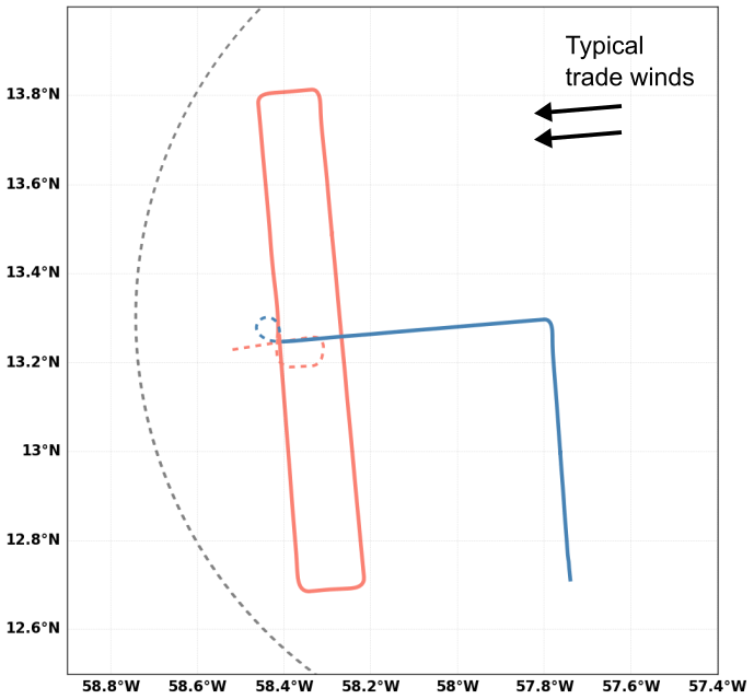
Figure 1 Schematic horizontal trajectory of the SAFIRE ATR 42 within the HALO circle (gray dashed lines) during EUREC⁴A. Maneuvers for alignment, ferry legs and other parts of the trajectory projection are not shown here. The R pattern is shown in red, and the L pattern is shown in blue.

During each SAFIRE ATR 42 flight, two to four rectangles were flown, generally around the cloud-base level, except when stratiform clouds were occurring higher up and a rectangle was also flown around the trade inversion level. In addition, two to four L patterns were flown, each pattern being composed of two straight legs of about 60 km (one along-wind and one across-wind) flown either near the top or the middle of the subcloud layer. These patterns aimed to explore the anisotropy of the turbulence and the organization, as well as the vertical structure of the boundary layer.

During a single HALO flight of about 9 h, the ATR 42 flew two flights (using a similar flight plan) with a short refueling in between. The repetitiveness of the flight plans makes it possible to consider all the flights to be members of the same statistical ensemble.

Table 1 describes each flight plan, together with some information about the mean wind within the subcloud layer and the types of clouds observed. It shows how, during the campaign, the conditions evolved from suppressed conditions, with only rare and thin cumulus clouds, toward more cloudiness and more vertical development. This was associated with a gradual strengthening of the mean wind in the subcloud layer. Note that flights RF01 and RF02 are not included in the table because they were electromagnetic interference (EMI) and test flights, and RF20 had no rapid measurements because of an inertial navigation system failure.

Table 1 Flight plan and wind conditions associated with each flight during the EUREC⁴A field campaign. The flight altitude is indicated between brackets, and the notations “cb”, “strati” and “surf” refer to cloud base, stratiform layer and surface, respectively. The wind conditions within the subcloud layer are inferred from the averaged airborne measurements over the L legs, including both the top and mid-subcloud layer (except for RF16, during which there was no L pattern). t_i and t_f are UTC times for the start and end of the flights, respectively.

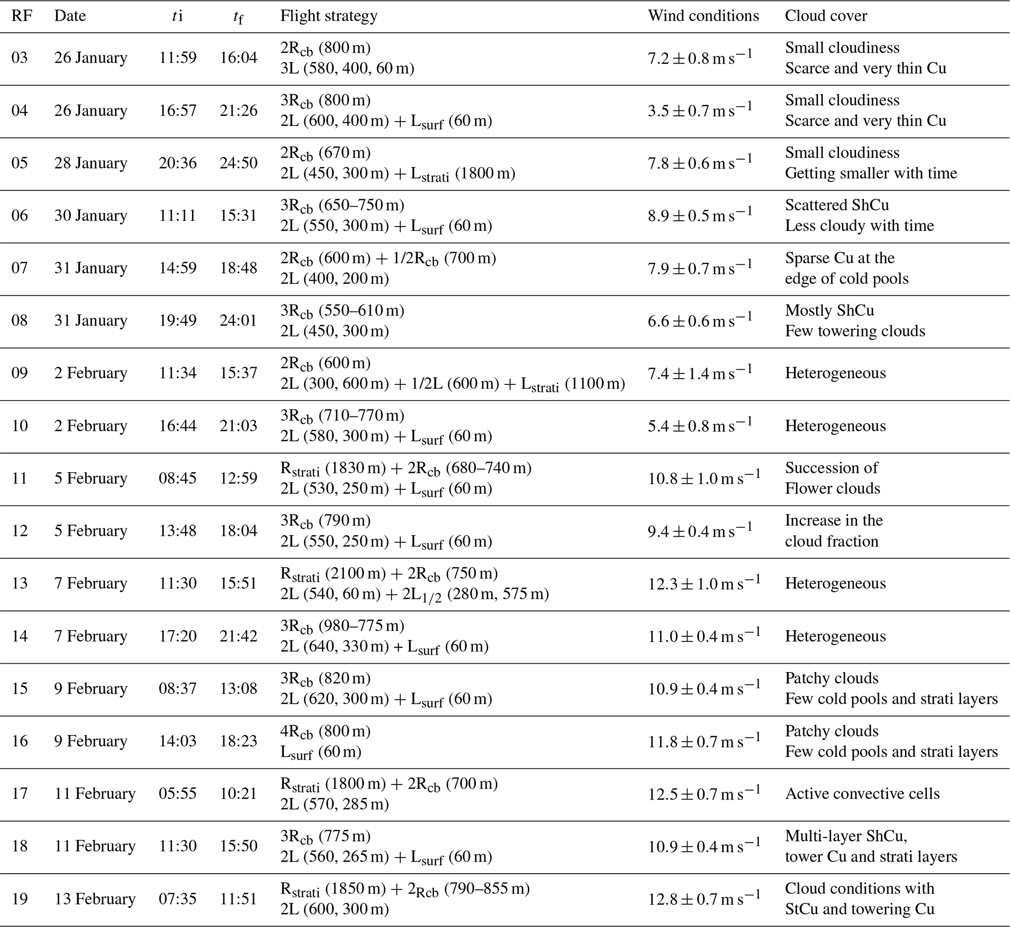
For the description of the cloud cover, the abbreviations are defined as follows. Cu: cumulus, ShCu: shallow cumulus, StCu: stratocumulus, Flower clouds: circular clumped patterns as introduced by Stevens et al. (2020).

3 Aircraft in situ instrumentation for high-rate thermodynamical measurements

The SAFIRE ATR 42 is a turboprop airplane initially used for commercial aviation, which has been profoundly modified for the purpose of atmospheric and environmental research. It is permanently instrumented with in situ basic measurements (thermodynamics, radiation, microphysics) and also has a large flexible payload capacity, which enables the use of a large number of in situ and remote sensing observations.

The core in situ instrumentation used during EUREC⁴A and the low-rate measurements (1 Hz) associated with it are described in Bony et al. (2017) and Stevens et al. (2021). The higher-rate measurements (25 Hz) are, to a large extent, based on the same instrumentation.

The SAFIRE ATR 42 is equipped for high-rate measurements of the three wind components of air motion, air temperature and air moisture. Initially acquired at various higher sampling rates consistent with the time response of the sensors, the final high-rate measurements of the meteorological variables were sampled at a common frequency of 25 Hz. For a true air speed of about 100 m s⁻¹, this corresponds to a sample spacing of approximately 4 m.

The three components of the wind are obtained by adding the velocity vector of the aircraft with respect to the Earth and the velocity vector of the air with respect to the aircraft. The ground velocity is measured with an inertial navigation unit (AIRINS, model 6005214 from iXblue company). The velocity of the air relative to the aircraft is computed from the measurement of the true air speed magnitude as well as the attack and side-slip angles, according to Lenschow (1986). The attack and side-slip angles are respectively deduced from the vertically aligned and horizontally aligned differential pressure measured on the five-hole nose radome with pressure transducers, according to the technique first described by Brown et al. (1983). The true air speed (TAS) is calculated from the measurement of the dynamical pressure and the static pressure. The static pressure is measured on the fuselage side with a Pitot tube and a pressure transducer. The dynamical pressure is obtained by subtracting the static pressure from the total pressure measured at the central radome hole. The velocity measurement and computation have proven to be reliable in numerous field campaigns (Lambert and Durand, 1998; Saïd et al., 2005, 2010).

Air temperature is retrieved from a platinum wire thermometer placed in a Rosemount housing (E102AL Rosemount), after correction for the adiabatic heating due to the air speed of the plane. During EUREC⁴A, temperature was also measured using two fine wires (Baehr et al., 2002) that were housed in a tubular antenna. The two platinum fine wires are housed in a tubular antenna from SFIM company (model T4113). They are more directly exposed to the stream but protected from radiation, which consequently should not have a significant impact.

Moisture fluctuations were measured with a krypton hygrometer Campbell KH20, which has been adapted for airplanes. Initially used for measurements on ground towers, this sensor was profoundly modified to be inserted into the housing of a former moisture sensor (Lyman-alpha hygrometer). The signal is calibrated based on reference slow (1 Hz) measurements of humidity. Here we use the Water Vapor Sensing System (WVSS2) for reference instead of the typical chilled-mirror sensor reference (General Eastern 1011). A Li7500 LI-COR sensor was used as a spare for fast humidity measurements. It was also adapted for aircraft measurements and previously used in the HyMeX (Estournel et al., 2016) and DACCIWA (Knippertz et al., 2015) field campaigns.

Due to several circumstances, some technical difficulties were encountered during the field campaign, especially during its first phase. In particular, a major issue concerned one of the radome pressure transducers, making it impossible to calculate the attack angle with the usual methodology. This strongly impacts the air vertical velocity estimates. As a consequence and due to the sensitivity of air motion measurements, the dataset discussed here does not include the vertical velocity for flights RF02 to RF08, nor any estimate related to it.

The KH20 also showed issues during this first phase, partly due to the particular conditions of the marine environment encountered during EUREC⁴A, which make it challenging to measure air moisture at fine scale. The drastic change in water vapor content from above the inversion (where relative humidity can be as dry as a few percent) to below cloud base (where relative humidity is generally higher than 80 %) was a challenge, and the spacing between the emitter and the receiver of the KH20 sensor has been adjusted. In the subcloud layer patterns, the sea salt loading of the KH20 sensor generated a significant loss of signal dynamics. An assiduous cleaning of the optics at the beginning of each flight allowed us to limit this loss of signal. Regarding the KH20 behavior, many technical issues were gradually solved and several improvements were made following the feedbacks at the end of each flight. Thus, the KH20 performances were significantly improved by the second phase of the campaign (flights RF09 to RF19). The calibration of moisture fluctuations, choice of reference slow measurement, and the relative performances of the KH20 and LI-COR are discussed further in Sect. 4.

As a consequence of those difficulties and after quality control, there are flagged or rejected data within the dataset. The second phase of the field, corresponding to flights RF09 to RF19, had much better-quality data.

4 Calibration and qualification of the fast humidity sensors

One of the current challenges of atmospheric turbulence measurements is the fast measurement of humidity, which remains difficult at frequencies higher than 1 Hz. For many years in the past, a robust and high-performance krypton hygrometer called Lyman-alpha was commonly used for the measurement of (uncalibrated) air moisture fluctuations (Buck, 1976; Saïd et al., 2010; Canut et al., 2010). Since the UV source of this sensor is not available anymore, one had to use another sensor. However, achieving a similar performance remains a challenge. Here, we use a KH20 krypton hygrometer, which has been recently adapted and installed on board the SAFIRE ATR 42.

In this section, we discuss the data calibration and control over stabilized legs of 5 min. This segmentation is a compromise to ensure the best sampling representativity and homogeneity (see Sect. 6 for more details).

The time series shown in Fig. 2a illustrates a comparison of uncalibrated fast measurements from the KH20 sensor with two slow sensors: the WVSS2 sensor and the 1011C mirror hygrometer. The WVSS2 measures the relative humidity in percent by absorption spectroscopy with a tunable diode. The 1011C hygrometer is a condensation hygrometer, which measures the dew point temperature. Absolute, relative and specific humidity are then inferred from dew point, temperature and pressure. To calibrate the fast sensor with the reference slow measurement of absolute humidity, both the slow and fast signals are initially low-pass-filtered at $\mathrm{1}/\mathrm{6}$ Hz, and then a linear regression is computed to obtain the calibration slope and the intercept to be applied to the fast signal. The quality of the calibration is assessed by the R-squared value (R²) of the linear regression between the low-pass signals of the reference sensor and of the fast sensor. One expects R² larger than 0.98 for high-quality signals of slow and fast measurements. Figure 2b shows the resulting calibrated signal converted to a water vapor mixing ratio and compared to the slow series of the same variable.

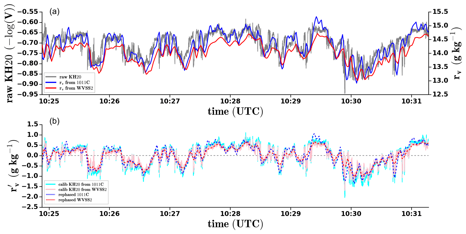
Figure 2 Example of humidity measurements and calibration during a leg (l1a) flown at z∼600 m on 13 February 2020 (RF19): (a) time series of (gray line) the raw uncalibrated signal of the fast KH20 sensor and the water vapor mixing ratio inferred from (blue line) the 1011C mirror hygrometer or (red line) the WVSS2 sensor. (b) Corresponding time series of the water vapor mixing ratio fast fluctuations derived from the KH20 calibrated signal and the reference slow measurements phased in time with the fast sensor from (cyan line) the 1011C mirror hygrometer and (pink line) the WVSS2 sensor.

4.1 Choice of slow sensor

The measurements of the two slow sensors exhibit differences which can impact the calibration. To optimize the choice of the slow reference and the calibration process, we considered the second phase of the campaign (flights RF09 to RF19), which had fewer technical issues and during which the KH20 showed a very good behavior in terms of time response and consistency with other moisture sensors. Figure 4a and b show the distributions of R² on all segments of flights RF09 to RF19 when using either the 1011C mirror hygrometer or the WVSS2 sensor as a reference, respectively. The R² values are significantly higher when the WVSS2 sensor is used as a reference. This reveals a better behavior of the WVSS2 sensor relative to the 1011C hygrometer. The latter, despite its shorter response time, showed more difficulties in following the large variability of air moisture encountered during EUREC⁴A, which added to the challenges of measuring air moisture in an environment with sea salt, clouds or even rain. This phenomenon can be noticed around 10:29:20 UTC in Fig. 2b and more clearly in Fig. 3, where the 1011C signal (dashed blue) shows several exaggerated peaks because it responded too slowly to the increasing and following fast leveling of moisture. This behavior is explained by its measurement principle, with condensation at the mirror surface, which requires time to recover by drying. This issue resulted in a positive bias of about 27 % in the estimated moisture variance when the KH20 was calibrated with the 1011C hygrometer. This bias is visible in Fig. 2b and even more clearly in Fig. 3b from the difference in fluctuation energy between the two signals.

Figure 3 Same as Fig. 2 for a leg (l1c) flown at z∼600 m on 13 February 2020 (RF19).

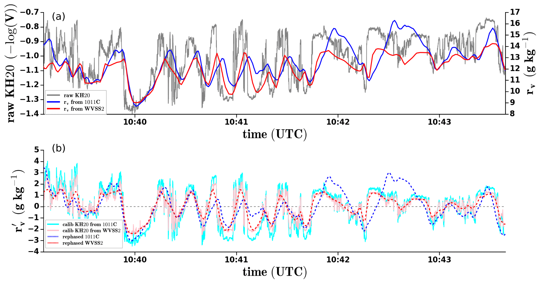
Figure 4 makes the distinction between legs flown within the subcloud layer (or MABL legs, associated with more homogeneous turbulence) and the rest of the legs. At cloud base, the turbulence is highly heterogeneous, with a mix of cloudy air, subcloud layer air and free tropospheric air. On the other hand, the legs flown higher up near the trade inversion level exhibit a very weak turbulence or an intermittent turbulence associated with individual clouds. The distributions do not show strong differences between one set and the other. This indicates that the calibration against WVSS2 actually works both in the MABL and above the subcloud layer.

Figure 4 Histograms of the linear regression R-squared value (R²) associated with the calibration of the KH20 fast humidity measurement with, as the reference slow measurement, (a) the 1011C mirror hygrometer, (b) the WVSS2 sensor and (c) the WVSS2 sensor phased in time with the fast sensor. The comparison is done for all flights from RF11 to RF19, considering either the entire set of legs or just the legs flown within the MABL. The vertical dashed line represents the R²=0.9 threshold.

The WVSS2 is a slower sensor than the 1011C hygrometer, with a time response of about 2.5 s against about 1 s. Due to this significant delay (that can be seen in Fig. 2a), we tested the impact of phasing the slow signal to the fast signal. Figure 4c shows the significant improvement obtained with this phasing: for most of the legs, R² is now larger than 0.95. Figure 2b shows the calibrated signal of the KH20 converted to a water vapor mixing ratio, along with the phased slow signal used for optimum calibration. Figure 5 shows that the phasing has only a small impact on the variance of moisture: it is only 1.7 % larger in the case of the phased slow signal, which is much smaller than the random error.

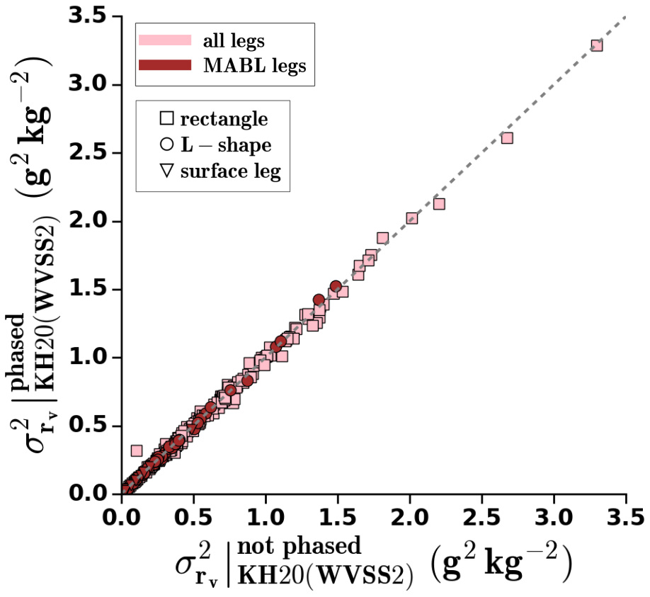
Figure 5 Variance of the water vapor mixing ratio computed with the KH20 sensor, after calibration with the WVSS2 sensor phased in time, versus the variance obtained when the WVSS2 sensor is not phased. The comparison is done for all flights from RF11 to RF19, considering either the entire set of legs or just the legs flown within the MABL. The markers refer to the different types of leg, as sketched in Fig. 1.

For a thorough qualification of the fast moisture measurements during EUREC⁴A, considering R-squared values is not sufficient. Indeed, even if the correlation with the slow signal is good, the sensor might not show the proper dynamics of the amplitude of the fluctuations (e.g., due to sea salt or to an inappropriate spacing between the emitter and the receiver). For this reason, we used as an additional index, the root mean squared error (RMSE), calculated between the low-pass-filtered calibrated signal ($\mathrm{1}/\mathrm{6}$ Hz) and the slow reference signal (also low-passed). The smaller this index, the better the agreement between the fast and slow sensors at large scales.

The quality of the fast humidity measurements is thus assessed with respect to two metrics: R² and RMSE. For each sensor (KH20 or LI-COR), we define a green, yellow or red flag with respect to the combination of criteria for those two metrics (Fig. 6). The high-quality (green) flag is defined by R²≥0.9 and RMSE<0.16. In contrast, the poor-quality (red) flag is defined by R²<0.6 or RMSE>0.6. All other combinations of those two metrics correspond to an intermediate yellow flag. Note that the threshold values used to define these criteria result from a sensitivity analysis that compares the moisture flux and the variance obtained with the KH20 or LI-COR sensors.

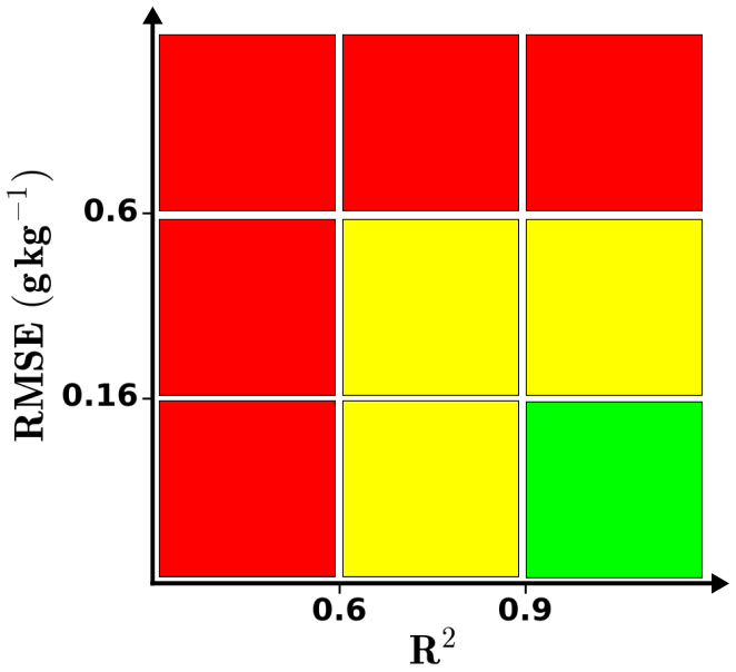
Figure 6 For each sensor (KH20 or LI-COR), the quality of high-rate humidity measurements is assessed against two metrics: R² (on the horizontal axis) and RMSE (on the vertical axis). The quality decreases from green to red.

4.2 Comparison of the KH20 and LI-COR sensors

During EUREC⁴A, two fast sensors were mounted on the SAFIRE ATR 42: the LI-COR sensor, which had been previously adapted to the airplane, and the KH20 sensor, which was adapted to the airplane more recently in the hope of improving the performance of the high-rate humidity measurements.

Figure 7a shows an example of time series from both sensors during a subcloud layer segment of flight RF19 after the calibration process discussed previously. First, it shows that the signal from the LI-COR sensor was associated with significant noise. This feature was present during the entire field campaign. In addition to this noise issue, the LI-COR showed appropriate moisture measurements at lower frequencies, consistent with good R-squared coefficients of the calibration (R²=0.99 for both KH20 and LI-COR in Fig. 7). The corresponding spectra of those series shown in Fig. 7b exhibit the noise issue of the LI-COR more clearly. In contrast, the KH20 shows a nice behavior of the spectra up to 6–8 Hz, notably showing the $-\mathrm{2}/\mathrm{3}$ slope in the inertial subrange. This means that this sensor can be used to study fine-scale processes.

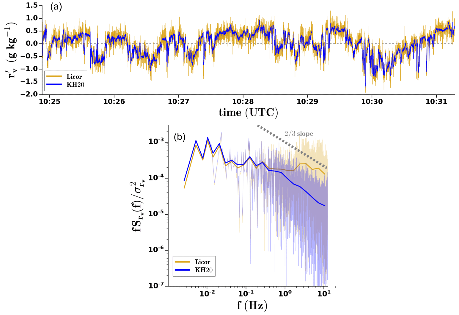
Figure 7 Comparison of LI-COR and KH20 signals on a leg flown at z∼600 m on 13 February 2020 (RF19): (a) time series of water vapor mixing ratio fluctuations from the LI-COR (in yellow) and from the KH20 (in blue). (b) Associated normalized energy density spectra. Smoothed spectra are indicated by thick solid lines.

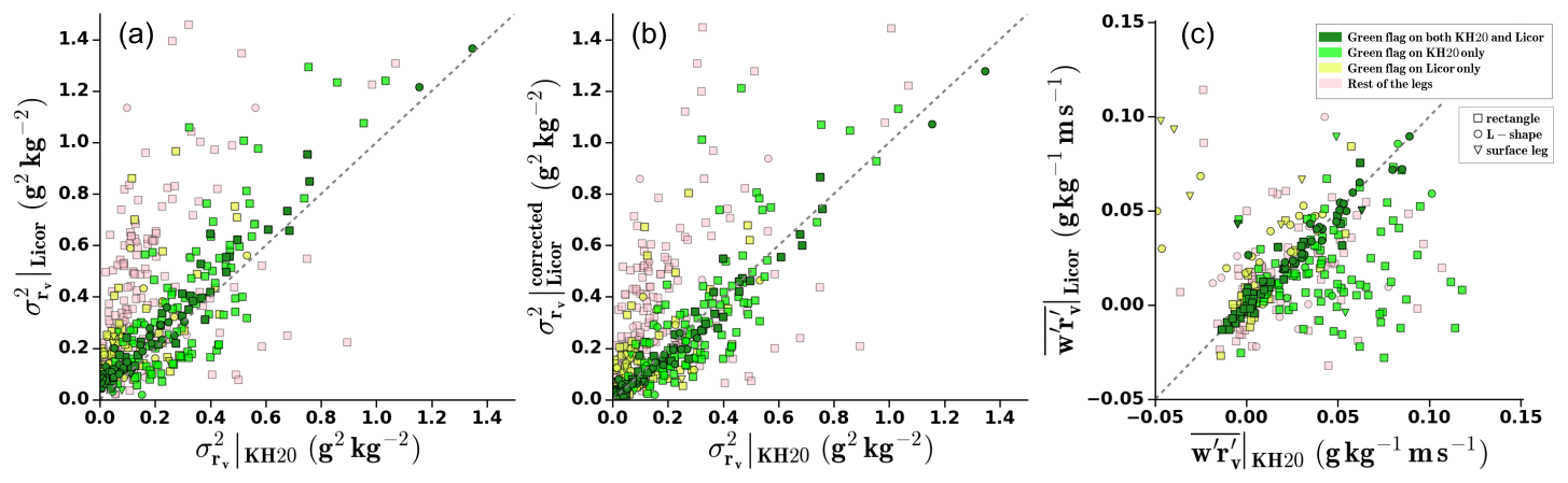
Figure 8 Humidity variances computed on 5 min segments for all the flights RF03 to RF19: (a) from the KH20 signals versus the LI-COR signals and (b) from the KH20 signals versus the LI-COR signal corrected for noise. (c) Moisture flux from the KH20 signal versus from the LI-COR signal for flights RF09 to RF19. The symbols correspond to the altitude of the leg. The dark green markers refer to legs with a good-quality calibration of humidity for both sensors. Bright green markers refer to legs with a good-quality calibration of humidity for the KH20 sensor only. The yellow–green markers refer to legs with a good-quality calibration of humidity for the LI-COR sensor only. Finally, the bright pink markers correspond to the rest of the legs.

The determination of the thresholds of R² and RMSE for the green flag introduced above was made such that the selected green-flagged legs showed good consistency between the KH20 and the LI-COR for the estimates of moisture variance and covariance. This is illustrated with Fig. 8. Consistently, when we consider only the legs with green flags for both sensors, the agreement on variance (Fig. 8a) and moisture flux (Fig. 8c) is very good, especially relative to the small intensity of turbulence found in EUREC⁴A and the large associated random errors.

The noise of the LI-COR signal naturally impacts the variance estimates, leading to an overestimation of about 0.05 g² kg⁻² (Fig. 8a). However, the LI-COR noise does not significantly impact the covariance estimates of vertical velocity with moisture ($\stackrel{\mathrm{‾}}{w^{\prime }{r}_{\mathrm{v}}^{\prime }}$), as shown in Fig. 8c, because the noise signal is not correlated with the vertical velocity. Moreover, the energy of the correlation mainly ranges over scales larger than those over which the noise predominates.

As a result of this analysis, the KH20 sensor is primarily used for turbulence moment estimates and analysis of the fine-scale processes. But in the case of strong failure of this sensor, the LI-COR is used as an alternative for the covariance estimates. The variances of the LI-COR were corrected for noise (Fig. 8b) by using the value of the autocovariance function of moisture fluctuations at the fifth lag as an estimate of the variance. The use of the first lag is common and adapted for taking account of uncorrelated noise (Lenschow et al., 2000, 2012), since the autocovariance at zero lag is equal to the variance of the signal plus the variance of the white noise. Here, we found that using the fifth lag was more appropriate due to slightly correlated noise and the need to find a best compromise. This means that we lose the amplitude of the fluctuations of scales smaller than 20 m.

We found that, generally, the KH20 sensor encountered issues in legs close to the surface due to sea salt. This is clearly shown in Fig. 8c, where the legs with a green flag for LI-COR only (yellow–green) all show larger covariances with LI-COR. In contrast, the LI-COR had more difficulties when the SAFIRE ATR 42 was crossing clouds or even rain during the “R” legs, while the KH20 behaved much better in those wet conditions. Indeed, in Fig. 8c, all the legs associated with a green flag for KH20 only show larger covariances with KH20 than for LI-COR.

In order to obtain the best estimate of the turbulent moments and fluctuations for each leg, they have been calculated using either one sensor or the other depending on their respective flags, with priority given to the KH20 sensor. This results in the definition of a combined flag as illustrated in Fig. 9. In total, over the 535 5 min segments, 241 segments are based on the KH20 with a green flag (green combined flag), 113 are based on the LI-COR with a green flag as an alternate (yellow combined flag), 153 are based on the KH20 or the LI-COR with a yellow flag (orange combined flag), and 28 are unusable (red combined flag). Therefore, the calculation of the turbulent moments associated with humidity is trustworthy for the green and yellow combined flags. Orange flags should preferably be avoided, and red flags are automatically invalidated. Finally, although the confidence in the calculation of turbulent moments for the yellow flag is good, the use of LI-COR fluctuations for studying fine-scale processes (e.g., with spectral analysis or probability density functions) should be avoided, as shown in Sect. 4.2. The KH20 sensor should be preferred because of its better description of the expected spectrum in the inertial range and its better recording of the amplitude and the distribution of the fluctuations.

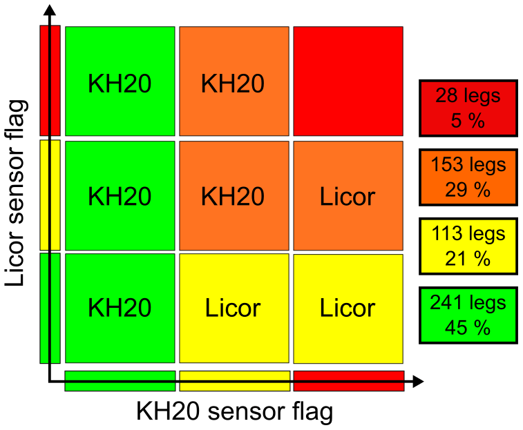
Figure 9 Definition of a combined flag for the humidity, depending on the KH20 and the LI-COR sensor quality flags. The number of segments and the associated percentage for each category of the combined flag are indicated in the boxes on the right. It refers to flights RF03 to RF19 for the short legs.

5 Qualification of the fast temperature sensors

On board the SAFIRE ATR 42, the temperature was measured by two sensors: a Rosemount probe and a fine wire. The typical and reference Rosemount temperature probe showed some issues during the field campaign, including spurious negative spikes that were not visible on the fine wire sensor. Those were not easily explained but are supposed to be inherent to the sensor itself. Rarely, large noise could also appear locally in the presence of cloud droplets. The housing of the Rosemount probe makes it difficult for the cloud droplets to penetrate the probe and to reach the sensor. However, should a droplet reach the sensor, it takes more time to dry out. In contrast, the fine wire is more exposed, but it recovers quickly. A usual weakness of the fine wire is its ability to break with shocks, in particular during takeoff or landing. During EUREC⁴A, the fine wires did not break and turned out to provide a better fine-scale signal than the Rosemount probe.

The two fine wires were installed starting with flight RF09 and calibrated with the Rosemount probe at 1 Hz for each flight. Both fine wires were consistent with the other, but one showed some noise that the other did not show at all. We consider only the latter here. We considered this measurement non-absolute and used it only for the study of temperature fluctuations. We calibrated the fine wire with the raw impact temperature of the Rosemount probe temperature as a reference, with one calibration per flight. The regression slope was very close to 1 (1.07 on average, with a standard deviation of 1.2 % over the 11 flights concerned). The most significant variability was found in the offset (coordinate at the origin of the regression line), which varied between −4.6 and −1.9 ^∘C, with a standard deviation of 2.6 ^∘C. This variation may be explained by the fine wire resistance varying with time due to oxidation. From this calibration and due to the incertitude of the housing features and recovery factor, we applied the same recovery factor of the Rosemount (0.98) to retrieve the static temperature from the impact temperature. Those results were similar to those found in the analysis of Baehr et al. (2002) for the same type of fine wire and the same antenna.

Figure 10a shows a time series of the temperature fluctuations derived from each sensor during a subcloud layer leg of RF19. The spikes of the Rosemount temperature probe signal were particularly numerous in this example. The comparison also reveals the shorter time response of the fine wire and its better ability to catch the small-scale variability. This is confirmed by the comparison of the spectra (in Fig. 10b), which shows how the fine wire temperature density energy spectrum (multiplied by the frequency) better follows the expected $-\mathrm{2}/\mathrm{3}$ slope in the inertial subrange.

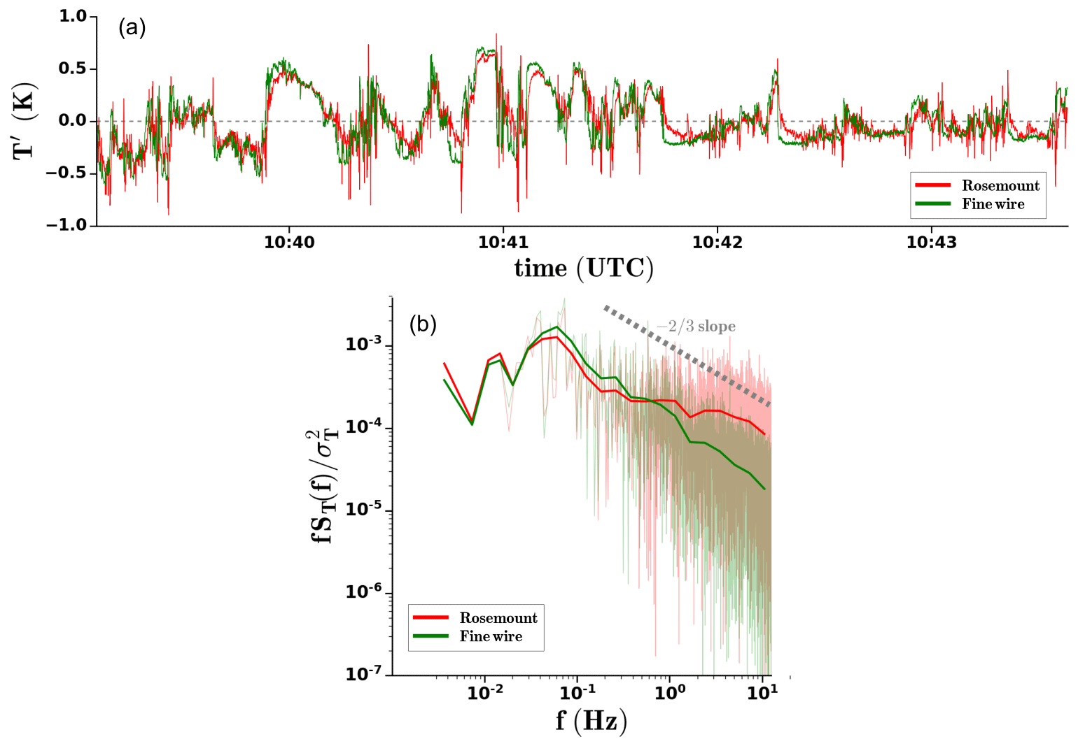
Figure 10 (a) Time series of the temperature fluctuations measured by the Rosemount probe (in red) and by the fine wire (in green) during a subcloud layer leg of RF19. (b) Corresponding density energy spectrum.

The covariance between temperature and moisture is further evidence of the larger relevance of the fine wire signal (Fig. 11). Temperature and moisture fluctuations are often well correlated: for example, an intrusion of air from above is associated with a drier and warmer structure (negative and positive fluctuations of moisture and temperature, respectively). Figure 11 shows that this correlation is higher when the temperature is measured by the fine wire than when it is measured by the Rosemount probe. It is partly explained by the fact that the temperature variance is larger with the fine wire, but also because the fine wire tracks the fine-scale fluctuations of temperature better than the Rosemount probe. For these reasons, the fine wire temperature signal was chosen during EUREC⁴A for the best estimate of the turbulent moments and fluctuations. The Rosemount probe temperature was used as a spare during the first part of the campaign and during a few R legs of RF17 and RF19 when the fine wire sensor was heavily impacted by cloud droplets. A green flag was associated with the fine wire use and a yellow flag with the use of the Rosemount probe.

Figure 11 Comparison of the covariance of temperature and moisture obtained when using the Rosemount probe temperature (y axis) and the fine wire temperature (x axis). In both cases, the calculation is based on the moisture fluctuations associated with a green flag.

6 Computation of turbulence moments and associated errors

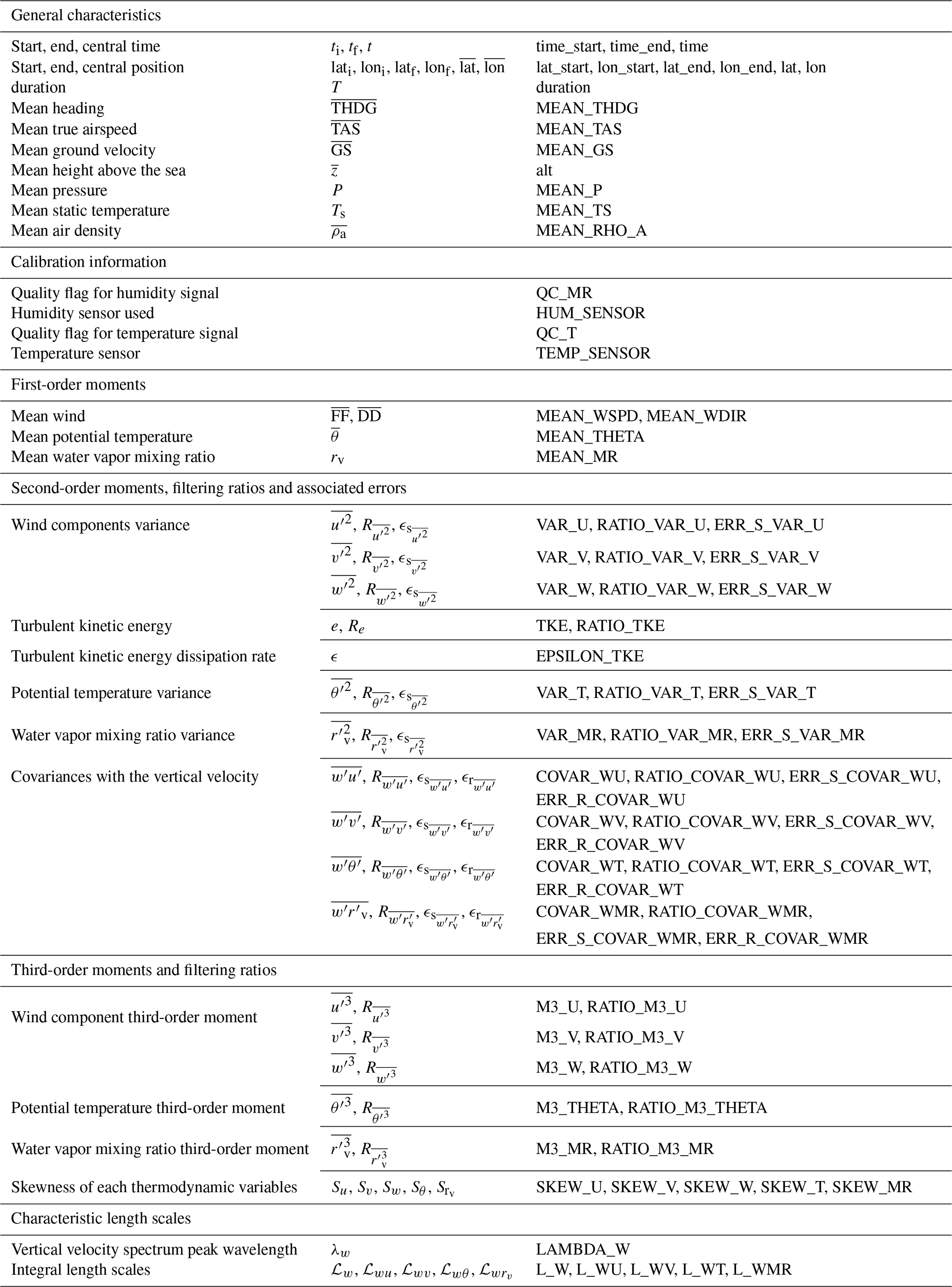
After control and calibration, the 25 Hz fluctuations are used to compute the turbulence moments and other characteristics of the MABL turbulence. The turbulent moments or characteristics evaluated for each leg are listed in Table 2.

Table 2 List of turbulent parameters calculated over each segment, their standard nomenclature and their names in the NetCDF files.

Only stabilized legs are considered for the turbulence data processing due to the increase in errors in basic measurements during turns or more generally during phases with varying flight attitude and speed. Moreover, to obtain a homogeneous statistical ensemble of turbulent moments associated with random and systematic error estimates, the straight horizontal legs are divided into segments of equal duration and length. Two types of segments are considered (Fig. 12): segments of 60 km and 10 min (referred to as “long legs”), which correspond to the length of an “L” branch, and segments of 30 km and 5 min (referred to as “short legs”). As suggested by Lenschow et al. (1994), 30 km long segments are a good compromise, as they are long enough to sample the structures which dominate the turbulent exchanges and short enough to explore the spatial variability from one leg to the other. Note that the short legs are occasionally adjusted within the subcloud layer (during L legs) to avoid water droplets (two segments of that kind).

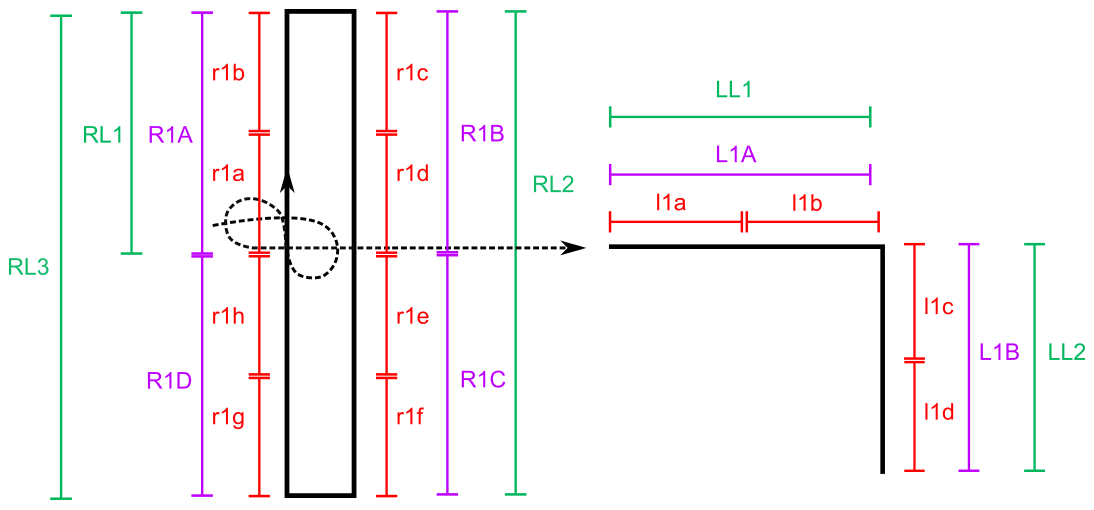
Figure 12 Schematic view of the segmentation of stabilized legs into segments of equal duration and length: 30 km, 5 min long segments (“short legs”, in red) and 60 km, 10 min long segments (“long legs”, in purple). Also reported are the “longest legs” (in green), which are the longest stabilized segments in one direction.

For each segment, the turbulent moments are calculated from two types of fluctuations time series: detrended series or high-pass-filtered series, with a cutoff frequency of 0.018 Hz (about 5 km wavelength). This filter is meant to remove the contribution of mesoscale features. The cutoff wavelength is chosen based on the co-spectra of the vertical velocity with all other variables (temperature, humidity, horizontal components) so that all turbulent scales contributing to the covariance are taken into account.

Figure 13 shows an example of the filtered time series of five variables: w^′, θ^′, $r_v^{\prime }$, $u_L^{\prime }$ and $v_T^{\prime }$. The prime symbol indicates a fluctuation relative to the mean value. Here $u_L^{\prime }$ and $v_T^{\prime }$ are respectively the longitudinal and lateral fluctuations of the horizontal wind relative to the mean wind over the considered leg. The longitudinal and lateral fluctuations of the horizontal wind relative to the aircraft, $u_x^{\prime }$ and $v_y^{\prime }$, are also calculated and made available in the dataset, as are the fluctuations of eastward and northward components. The use of one or the other referential depends on the purpose of the turbulence data analysis. In all three referentials, the vertical velocity is taken positive upward, and the referential systems are direct and orthogonal.

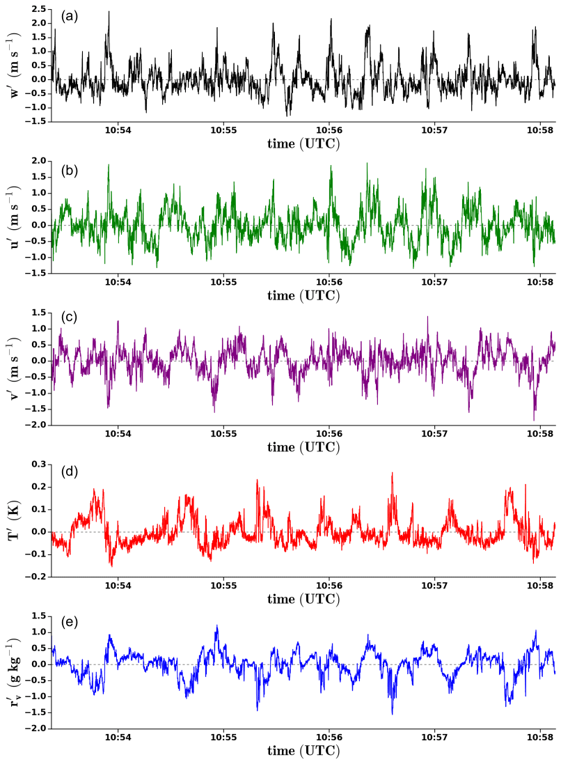
Figure 13 Time series of the filtered fluctuations of (a) vertical velocity, (b) wind velocity component longitudinal to the wind, (c) wind velocity component transverse to the wind, (d) potential temperature and (e) water vapor mixing ratio during a leg flown at z∼275 m on 13 February 2020 (RF19).

The second- and third-order turbulent moments are computed with the eddy correlation method. The covariance of two variables x and y is defined as

$$\begin{array}{}\text{(1)}& \stackrel{\mathrm{‾}}{x^{\prime }{y}^{\prime }}={\displaystyle \frac{\mathrm{1}}{T}}\underset{\mathrm{0}}{\overset{T}{\int }}{x}^{\prime }\left(t\right)y^{\prime }\left(t\right)\mathrm{d}t,\end{array}$$

where T is the duration of the leg. From the variances of u, v and w, the turbulent kinetic energy (TKE) is calculated as $\text{TKE}=\frac{\mathrm{1}}{\mathrm{2}}({\mathit{\sigma }}_u^{\mathrm{2}}+{\mathit{\sigma }}_v^{\mathrm{2}}+{\mathit{\sigma }}_w^{\mathrm{2}})$. Third-order turbulent moments are also computed, enabling the calculation of the skewness of a variable x:

$$\begin{array}{}\text{(2)}& S_x={\displaystyle \frac{\stackrel{\mathrm{‾}}{{x^{\prime }}^{\mathrm{3}}}}{{\left(\stackrel{\mathrm{‾}}{{x^{\prime }}^{\mathrm{2}}}\right)}^{\mathrm{3}/\mathrm{2}}}}.\end{array}$$

For both second-order and third-order moments, the ratio, denoted as R in Table 2, between the moment obtained without high-pass filtering (fluctuations obtained only by detrending the original series) and that obtained after high-pass filtering is computed. This index provides information about the stationarity and homogeneity of a sample. For a perfectly homogeneous and stationary sample with no impact of mesoscale or sub-mesoscale structures, this ratio should theoretically be equal to 1. It is often close to 1 for vertical velocity variance but can be much larger for other variables and for covariances.

Characteristic length scales suitable to describe the turbulence field are also computed, such as the wavelength of the vertical velocity spectrum peak or integral length scales. The length scale of the maximum spectral density energy of vertical velocity is obtained by fitting an analytical spectrum of the form $fS\left(f\right)=\frac{f{S}_{\mathrm{0}}}{\mathrm{1}+\mathrm{1.5}(\frac{f}{f_{\mathrm{0}}}{)}^{\mathrm{5}/\mathrm{3}}}$, where f is the frequency, and S₀ and f₀ are fitted to the observed vertical velocity spectra (Lambert and Durand, 1999; Attie et al., 1999). Depending on purpose, more complex analytical spectra may be used to estimate the wavelength of maximum spectral energy (see, e.g., Kristensen et al., 1989; Lothon et al., 2009 or Brilouet et al., 2017) and other definitions (e.g., Pino et al., 2006). This one is chosen for the sake of simplicity.

The integral length scale of a variable x is estimated as the integral of the normalized autocorrelation function from zero lag (τ=0) to the first zero (τ₀) of the function (Lenschow et al., 1994):

$$\begin{array}{}\text{(3)}& {\mathcal{L}}_x={\displaystyle \frac{\mathrm{1}}{\stackrel{\mathrm{‾}}{{x^{\prime }}^{\mathrm{2}}}}}\underset{\mathrm{0}}{\overset{{\mathit{\tau }}_{\mathrm{0}}}{\int }}\stackrel{\mathrm{‾}}{x^{\prime }\left(t\right)x^{\prime }(t+\mathit{\tau })}\mathrm{d}\mathit{\tau }.\end{array}$$

The turbulent kinetic energy dissipation rate (ε) is estimated from the vertical velocity energy spectrum S_w in the inertial subrange (Lambert and Durand, 1998) based on the Kolmogorov formulations: $S_w\left(k\right)=\frac{\mathrm{4}}{\mathrm{3}}\mathit{\alpha }{\mathit{\epsilon }}^{\mathrm{2}/\mathrm{3}}{k}^{-\mathrm{5}/\mathrm{3}}$, where k is the wavenumber ($k=\frac{\mathrm{2}\mathit{\pi }}{\text{TAS}}f$) and α is the Kolmogorov constant, taken as α=0.52 (Fairall and Larsen, 1986).

The reliability and accuracy of the observed turbulent moment estimates can be assessed based on sampling and filtering conditions. As introduced by Lenschow et al. (1994), using high-pass-filtered and finite-length samples generates an error which can be decomposed into two contributions: a systematic error (ϵ_s) and a random error (ϵ_r). The systematic error reflects the loss of information due to the high-pass filtering and can be estimated as the difference between the covariance of the detrended series (F_det) and the covariance of the high-pass-filtered series (F_fil):

$$\begin{array}{}\text{(4)}& {\mathit{ϵ}}_{\mathrm{s}}={\displaystyle \frac{F_{\det }-F_{\mathrm{fil}}}{F_{\det }}}.\end{array}$$

The random error is generated by the finite length of the sample and is therefore inherent in the measurement and cannot be removed. For a covariance between two variables x and y, the associated random error can be estimated by

$$\begin{array}{}\text{(5)}& {\mathit{ϵ}}_{\mathrm{r}}=\sqrt{{\displaystyle \frac{\mathrm{2}{\mathcal{L}}_{xy}}{L}}}\sqrt{\mathrm{1}+{\displaystyle \frac{\mathrm{1}}{r_{xy}^{\mathrm{2}}}}},\end{array}$$

where ℒ_xy is the integral length scale of $x^{\prime }{y}^{\prime }$, L the length of the leg, and r_xy the correlation coefficient between x and y.

7 Available dataset

The dataset includes two kinds of data.

1. Moments. The turbulent moments are calculated over each segment. The data are stored in NetCDF files (with one file per flight) for the three sets of short (30 km) and long (60 km) segments as well as over the longest possible segments of stabilized legs. However, one should note that these “longest” segments have different lengths that range from 60 to 125 km.

2. Fluctuations. The time series of fluctuations over each segment, filtered and detrended only, are made available to enable specific analyses or estimates of the turbulent moments through an alternative approach. There is one NetCDF file per segment and per flight.

Note that the fluctuations and moments over the longest possible segments are also made available, even if this last set is composed of segments of different lengths (from 60 to 125 km). It enables any user to work on the longest series of calibrated fluctuations for the entire stabilized legs. Of course, moments of R legs of 125 km are likely still more heterogeneous and should be considered only in specific strict conditions.

For both the turbulent fluctuations and turbulent moments, two levels of data processing are considered.

• Level 2. All files of turbulent moments and fluctuations are calculated for each sensor of temperature and humidity.

• Level 3 (or “best estimates'). Turbulent moments and fluctuations are derived from the sensors (or their combination) that have the best quality flags for the leg under consideration (the flags are described in Sects. 4 and 5); for each leg, they are considered as the best estimates of moments and fluctuations given the available instrumentation.

Table 3 explains the file nomenclature using Fig. 12 for the naming of each segment. For each flight, a YAML file is provided together with the dataset that defines the start and end times of each flight segment.

Table 3 File nomenclature. YYYYMMDD corresponds to the flight date (e.g., 20200202), NN to the flight number (e.g., 09), LEG to the segment identifier (e.g., R2B or l2c) and LEVEL to the level of data processing (L2 or L3).

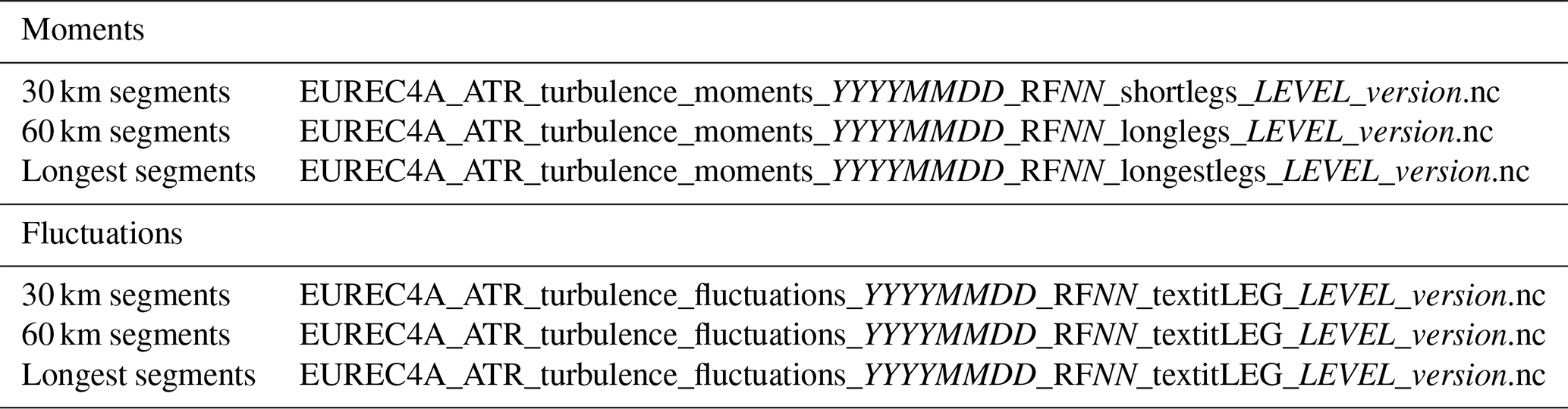
Figure 14 summarizes the availability and the quality of the high-rate data associated with each key variable. Based on the quality control described in Sects. 5 and 6 for temperature and moisture, it displays the proportion of legs within each flight that are associated with a green flag, as established on the basis of the L3 “short legs” dataset. This table shows how the quality of the measurements improved in the second phase of the field campaign (from RF09), with the best quality and availability achieved from RF15 onwards.

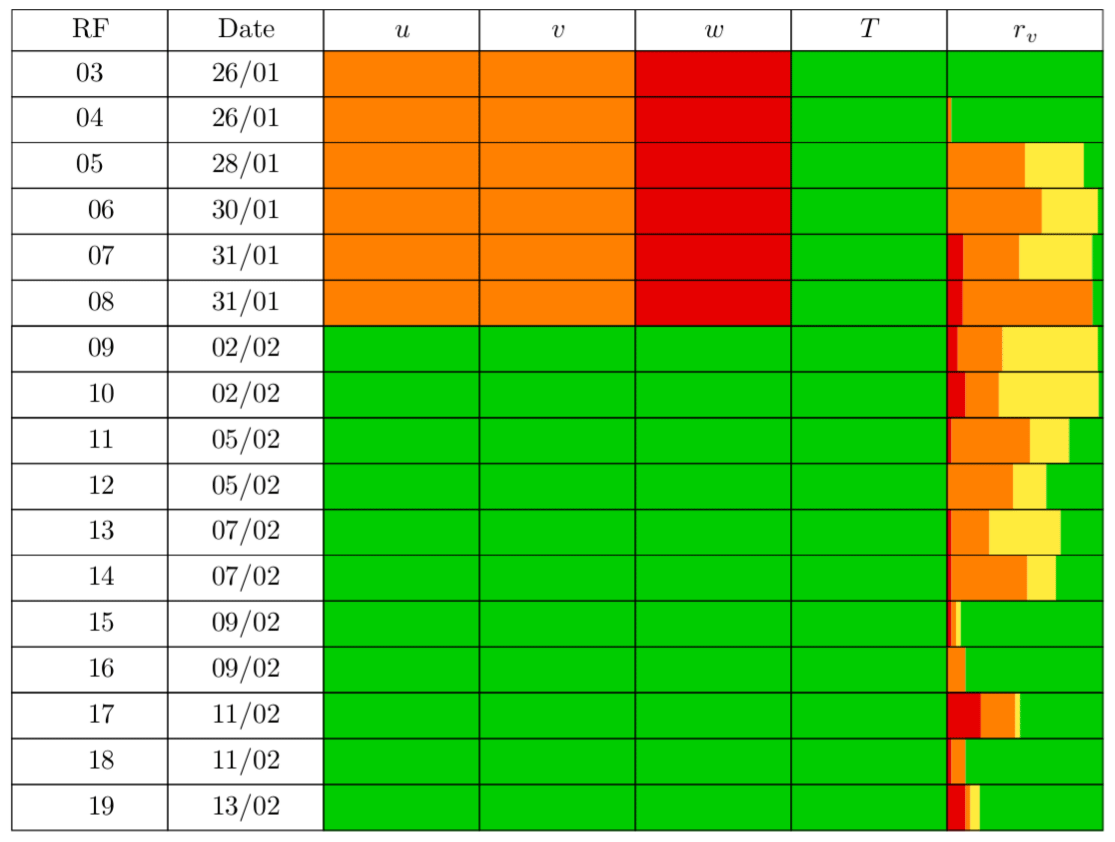
Figure 14 Quality flags associated with the turbulent data for each SAFIRE ATR 42 flight during the campaign. The data quality increases from red (poor quality) to orange, yellow and green (high quality). For moisture and temperature, the flag is the combined flag described in Sects. 4 and 5, considering the short legs of L3 data.

As an illustration of the dataset, Fig. 15 shows an overview of the vertical profiles of variances for the entire field experiment (RF03 to RF19). The profiles are normalized by the lifting condensation level (LCL), estimated here as the flight altitude of the rectangle at the cloud base minus 50 m. Overall, the turbulence is weak in the subcloud layer during EUREC⁴A. As expected in an MABL, the variance of vertical velocity is maximum within the first half of the subcloud layer, and the variance of the horizontal wind is larger near the sea surface. The variances of temperature and moisture are maximum near cloud base and the entrainment layer, and they are minimum close to the surface. The very large scatter of the turbulent moments on R legs flown around cloud base likely reflects the large heterogeneity of the samples, related to the crossing of clouds and the mix of air masses of very different origins and characteristics (including non-turbulent air masses). Over these legs, the moments need to be taken with caution because their definition assumes a homogeneous sample, which is a condition rarely met at cloud base.

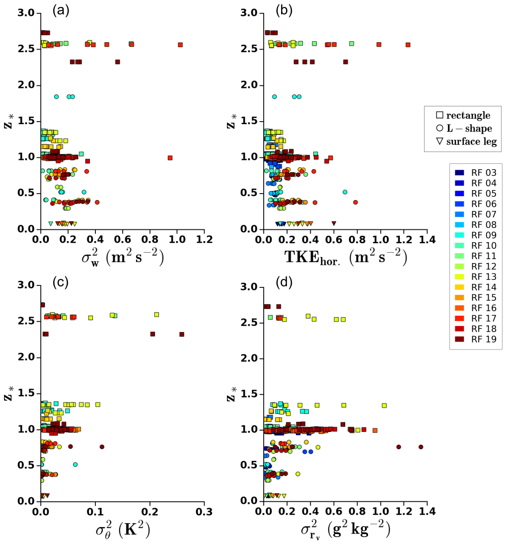
Figure 15 Normalized vertical profiles of the variance of (a) vertical velocity, (b) horizontal turbulent kinetic energy, (c) temperature and (d) water vapor mixing ratio. Flight numbers are indicated in the top right box. For the water vapor mixing ratio, only the legs with a green or a yellow combined flag have been considered. The normalized altitude z_* is defined by $z/\text{LCL}$ with LCL, the lifting condensation level.

Finally, Fig. 16 shows, for flights RF09 to RF19, the vertical profiles of the covariance of the vertical velocity with temperature (Fig. 16a) or moisture (Fig. 16b), as well as their corresponding systematic and random errors. Around cloud base ($z_{*}\sim \mathrm{1}$), the random and systematic errors are very large. This is explained by the large heterogeneity of the samples at this level and indicates that the vertical flux estimates are mostly relevant below cloud base.

Figure 16 Normalized vertical profiles of (a) the heat flux, (b) the moisture flux, systematic error (c) for the heat flux, systematic error (d) for the moisture flux, random error (e) for the heat flux and random error (f) for the moisture flux. Flight numbers are indicated in the top right box. The normalized altitude z_* is defined by $z/\text{LCL}$ with LCL, the lifting condensation level.

The sensible heat flux is very small near the surface (likely due to the small air–sea temperature difference) and changes sign with height, consistent with the entrainment near cloud base. The moisture flux is more significant, with a large value near the surface and an overall decrease in the flux with height.

For both the heat flux and the moisture flux, the systematic error can be particularly large. This is largely due to the small fluctuations observed, resulting in very weak fluxes. Inside the MABL, the random error increases with altitude, partly related to the growth of the turbulent eddies. The profiles are similar to those found by Brilouet et al. (2017) during the HyMeX campaign over the Mediterranean Sea, which took place in much stronger wind conditions than here. Like in HyMeX, we find larger errors in the heat flux than in the moisture flux due to the more significant moisture fluctuations.

On the R legs above the MABL, the errors display a wide variability and potentially large values. This again reflects the high heterogeneity of the samples and the influence of the mesoscales at this height.

8 Data availability

The dataset is available at https://eurec4a.aeris-data.fr/ (last access: 6 July 2021, Lothon and Brilouet, 2020, https://doi.org/10.25326/128).

9 Conclusions

This paper presents the EUREC⁴A turbulent dataset that has been produced based on the high-rate in situ measurements of wind, temperature and moisture from the SAFIRE ATR 42. It explains the data processing strategies, the calibration methodologies, the procedures of quality control applied to the 25 Hz temperature and moisture measurements, and the methods used to estimate the turbulent moments and their associated errors.

The redundancy of temperature and moisture sensors on board the aircraft enabled us to overcome the failure of one or the other sensor and to optimize the data processing. All turbulent moments and time series of turbulent fluctuations are associated with some information about the sensor(s) from which they are derived, plus a quality flag. These data constitute the Level-2 dataset. In addition, a Level-3 dataset provides an ensemble of best estimates of the turbulent moments and fluctuations over each stabilized leg of the SAFIRE ATR 42 flights.

Considering our analysis of the data as well as the flight strategy and conditions, we make the following remarks and recommendations to future users of this dataset.

• The data collected at cloud base over the R legs or segments should be used with great caution. First, the presence of cloud droplets or rain may affect the performance of the high-rate sensors. In addition, at this level the aircraft probes very contrasting air masses, including clouds and cloud-free air originating from the subcloud layer or entrained from above. The large heterogeneity of the samples makes the calculation of turbulent moments quite uncertain around cloud base. However, the turbulent fluctuations remain relevant and can be used for specific analyses such as conditional sampling, object approaches or case studies.

• The moisture fluctuations measured by the LI-COR sensor and the temperature fluctuations measured by the Rosemount probe exhibit limitations at very fine scales. The variance and covariance estimates are not affected by these limitations, but we recommend that the spectral or distribution analyses of the turbulent fluctuations primarily use the data from the KH20 moisture sensor and from the fine wire temperature sensor.

• Owing to the weakness of the turbulent fluxes during EUREC⁴A, the turbulent moment estimates are associated with large systematic and random errors. This, added to the limited vertical sampling of the MABL, suggests that extrapolating sea surface turbulent fluxes from this dataset would not be accurate.

Despite these issues and the technical difficulties encountered at the beginning of the campaign, a rich and quality-controlled dataset has been produced based on the high-rate measurements of the SAFIRE ATR 42 that will make it possible to study the turbulence of the MABL during EUREC⁴A.

These data will be used to characterize the structure and the variability of the subcloud layer and the level of organization encountered underneath the clouds. Used jointly with the other EUREC⁴A datasets from aircraft, balloons or unmanned aerial vehicles, they will help to decipher the nature of cloud–circulation interactions and to identify the roots of the shallow convective organization. They will also help evaluate the ability of large-eddy simulations to predict the characteristics of turbulence within the subcloud layer of trade-wind regimes for a range of large-scale conditions.