the Creative Commons Attribution 4.0 License.
the Creative Commons Attribution 4.0 License.
 | 06 Jan 2021
Winter atmospheric boundary layer observations over sea ice in the coastal zone of the Bay of Bothnia (Baltic Sea)
Marta Wenta
David Brus
Konstantinos Doulgeris
Ville Vakkari
Agnieszka Herman
The Hailuoto Atmospheric Observations over Sea ice (HAOS) campaign took place at the westernmost point of Hailuoto island (Finland) between 27 February and 2 March 2020. The aim of the campaign was to obtain atmospheric boundary layer (ABL) observations over seasonal sea ice in the Bay of Bothnia. Throughout 4 d, both fixed-wing and quad-propeller rotorcraft unmanned aerial vehicles (UAVs) were deployed over the sea ice to measure the properties of the lower ABL and to obtain accompanying high-resolution aerial photographs of the underlying ice surface. Additionally, a 3D sonic anemometer, an automatic weather station, and a Halo Doppler lidar were installed on the shore to collect meteorological observations. During the UAV flights, measurements of temperature, relative humidity, and atmospheric pressure were collected at four different altitudes between 25 and 100 m over an area of ∼ 1.5 km2 of sea ice, located 1.1–1.3 km off the shore of Hailuoto's Marjaniemi pier, together with orthomosaic maps of the ice surface below. Altogether the obtained dataset consists of 27 meteorological flights, four photogrammetry missions, and continuous measurements of atmospheric properties from ground-based stations located at the coast. The acquired observations have been quality controlled and post-processed and are available through the PANGAEA repository (https://doi.org/10.1594/PANGAEA.918823, Wenta et al., 2020). The obtained dataset provides us with valuable information about ABL properties over thin, newly formed sea ice cover and about physical processes at the interface of sea ice and atmosphere which may be used for the validation and further improvement of numerical weather prediction (NWP) models.
- Article
(12309 KB) - Full-text XML
- BibTeX
- EndNote


Small-scale processes at the atmosphere–sea-ice–ocean interface are considered crucial to improve the performance of numerical weather prediction (NWP) models for the polar regions (Vihma et al., 2014). Sea ice, due to its low conductivity, isolates the ocean from the atmosphere and blocks the exchange of heat and moisture. However, due to wind forces, ocean currents, and internal pressure, the sea ice surface is not homogeneous but covered with ridges, cracks, and leads. All those features, in particular areas of open water or very thin ice, affect the properties of the overlying atmospheric boundary layer (ABL) both locally and regionally (e.g., Manucharyan and Thompson, 2017; Wenta and Herman, 2018, 2019; Batrak and Müller, 2018) and play an important role in sea ice dynamics and the evolution of seasonal sea ice extent (e.g., Horvat and Tziperman, 2015; Zhang et al., 2018). In situ observations of ABL properties over sea ice are essential for expanding our knowledge about physical processes (heat and momentum exchange, vertical mixing, fog and cloud formation, etc.) at the interface of the ocean, sea ice, and atmosphere and for the development of parameterizations necessary for the improvement of NWP models.
For many years, observations of the ABL over inhomogeneous sea ice have focused on satellite remote sensing (e.g., Qu et al., 2019), manned aircraft (e.g., Frech and Jochum, 1999; Brümmer, 1999; Tetzlaff et al., 2015), and expensive field campaigns (LEADEX, SHEBA; LeadEx Group, 1993; Uttal et al., 2002). While those data sources considerably increased our understanding of sea ice–atmosphere interactions (Vihma et al., 2014), there are still many gaps in the observations of the submesoscale processes at the interface of sea ice and the ABL. An approach that allows us to overcome many of the shortcomings of earlier field campaigns in the polar regions are unmanned aerial vehicle (UAV) operations. The usage of UAVs in harsh conditions associated with cryospheric studies has been continuously increasing throughout the last 15 years (Gaffey and Bhardwaj, 2020; Bhardwaj et al., 2016) as they provide an opportunity to reach previously inaccessible areas and to obtain 3D observations of the ABL. Formerly, such measurements were either impossible or too expensive and required several measuring platforms instead of one. The ABL and sea ice properties have already been a subject of several UAV campaigns focusing on the marginal sea ice zone (MIZOPEX; Zaugg et al., 2013), polynyas (Knuth. et al., 2013; Cassano et al., 2016), and the ABL structure offshore (deBoer et al., 2018). Another relevant campaign employing UAVs for observations of the stable atmospheric boundary layer over sea ice is “Innovative Strategies for Observations in the Arctic Atmospheric Boundary Layer” (ISOBAR) (Kral et al., 2018, 2020) which took place at and off the coast of Hailuoto island (Finland), i.e., the location of the present study. The main focus of ISOBAR was the study of the vertical structure of the stable boundary layer over ice. Overall, considering different surfaces (sea ice type and extent) and synoptic weather conditions, as well as time of the year, both campaigns, HAOS (Hailuoto Atmospheric Observations over Sea ice) and ISOBAR, are in many respects complementary and contribute to extending the still limited amount of available ABL data over thin seasonal sea ice.
The main goal of HAOS was to study the ABL response to sea ice surface inhomogeneities at different times of the day. Due to the very warm winter of 2019/20 and the associated exceptionally small sea ice extent in the Bay of Bothnia (and in the Baltic Sea in general) in the first months of 2020, the number of potential locations that would fit the purpose of our research was very limited. Eventually, after monitoring the development of weather and sea ice conditions throughout February 2020, the westernmost point of the Finnish island of Hailuoto (Fig. 1c), around the small harbor of Marjaniemi, was chosen as the most suitable location. The island is situated ∼ 20 km from the city of Oulu in the northeastern part of the Bay of Bothnia. During the period of interest, the waters surrounding Hailuoto to the north, east, and south were covered with landfast ice, as is typical for this region in February. Importantly, throughout the first 2 months of 2020, the edge of the sea ice cover was located only a few hundred meters off the coast. Consequently, the drifting ice pack that developed seawards from the landfast ice zone at the end of February, interesting from the point of view of the HAOS campaign, was within reach of our UAVs (Fig. 2). In short, the following factors influenced the choice of location of our study area: (i) accessibility of the site and availability of all necessary infrastructure, (ii) the exposed location of the island relative to the main coastline in that area, with Marjaniemi at its westernmost point, outside of the continuous zone of fast ice, and (iii) the presence of drifting sea ice pack within a short distance from the harbor, ensuring varying sea ice conditions in terms of floe size, ice thickness, etc. during the period of the campaign.
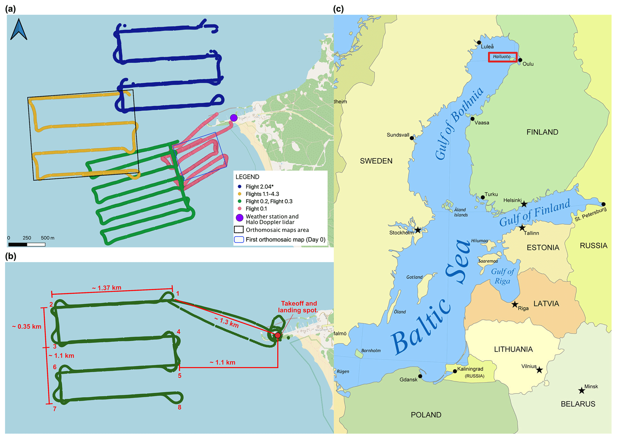
Figure 1(a) Flight paths during the HAOS campaign, flight labels as in Table 1. (b) The flight path of the meteorological measurement mission (Table 1; flights 1.1–4.3) with distances from the takeoff and landing spot close to Marjaniemi lighthouse pier. (c) The Baltic Sea with the highlighted location of Hailuoto.
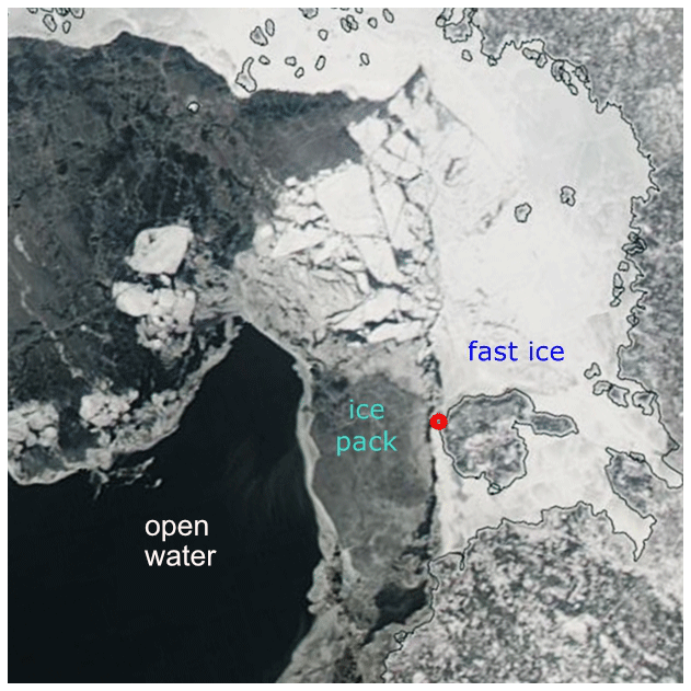
Figure 2Sea ice conditions in the inner parts of the Bay of Bothnia on 28 February 2020 (Day 1 of the campaign): MODIS Aqua image with marked fast ice, ice pack, and open water areas. The red dot shows the location of the Marjaniemi harbor.

Figure 3(a) UAV-UG1. (b) Telemetry screen for FPV real-time on-screen display of the UAV-UG1 performance. (c) DJI Mavic 2 Pro during flight. (d) Ground meteorological measurements.
Table 1Meteorological flights performed by UAV-UG1 with minimum and maximum values of measured parameters.
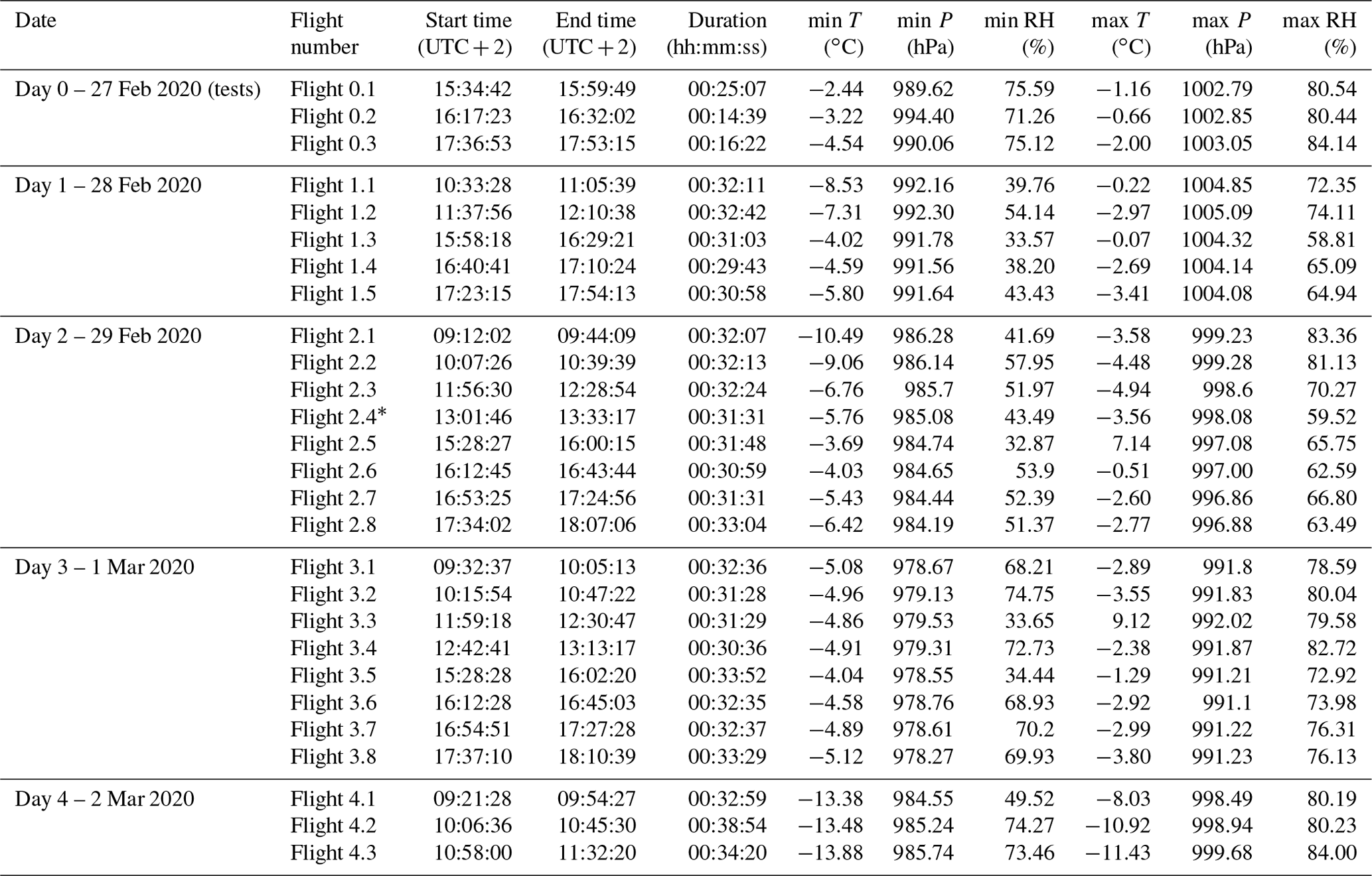
Between 27 February and 2 March 2020, a series of UAV flights were undertaken off the Marjaniemi harbor (Fig. 1a, b), which are accompanied by continuous ground-based observations of the lower atmosphere. Two different small UAVs were used: a fixed-wing UAV (called UAV-UG1) and a multi-rotor DJI Mavic 2 Pro. Apart from initial tests on 27 February, a total number of 23 UAV-UG1 flights took place, each covering the same area of 1.37 km×1.1 km, located 1.3–1.1 km from the starting/landing point at Hailuoto's Marjaniemi pier. The second, multi-rotor drone took overlapping aerial images of sea ice over the same area which were later used to create orthomosaic maps. In addition, a meteorological station and a Halo Doppler lidar instrument were installed at the pier (position: 65.039684∘ N, 24.555065∘ E), and they collected data throughout the whole campaign. A detailed description of all instruments and the measurement methodology are provided in the following sections.
2.1 Small UAV meteorological profiling
The small unmanned aerial vehicle (sUAV) platforms (UAV-UG1 and UAV-UG2, UG meaning the University of Gdansk) used during the HAOS campaign were built around the ZOHD Nano Talon fixed-wing V-tail airframe (Fig. 3a). The sUAV was developed at the Finnish Meteorological Institute (FMI) as an inexpensive measurement platform to operate in a variety of conditions. The Nano Talon is a small pusher-propeller aircraft with an 860 mm wingspan and all-up weight less than 1.5 kg. The maximum endurance of these aircrafts is about 60 min using 16.8 V, 3200 mAh rechargeable lithium-ion (Li-ion) batteries. Flights were carried out using a flight controller (Matek F405 wing) with the ArduPilot software. The propulsion system that consisted of 1870 kV brushless motors, 30 A electronic speed controllers, and 6 inch (0.1524 m) (3 inch pitch) propellers was used for both rotorcraft. In HAOS, all flights were conducted with the UAV-UG1 platform, having UAV-UG2 as a spare. The ground radio controller and UAV communicated via 868 MHz radio frequency with a range of more than 10 km. The aircraft utilized a first-person viewer (FPV) video link at 5.8 GHz, which enabled visual monitoring of the UAV performance with real-time on-screen-display (OSD) telemetry (Fig. 3b). All flights during the HAOS campaign were completed as autopilot-guided missions except for takeoff and landing operations which were under the control of an operator.
The platform carried a pair of meteorological sensors – Bosh BME280; P (hPa), T (∘C), and RH (%) – for measurements of the atmospheric state and the redundant GPS unit – long (deg), lat (deg), and alt (meters ± mean sea level) – both connected to a Raspberry Pi Zero W. The BME280 sensors were attached to each side of the aircraft fuselage under each wing (Fig. 3a). The attachment of the sensors was done via 3D-printed housing with the distance from the fuselage about 1.5 cm, allowing free airflow around the sensor and shielding it from the solar radiation. The BME280 sensor has a manufacturer-stated response time and accuracy of 6 ms and ±1 hPa for pressure, 1 s and ±0.5 ∘C for temperature, and 1 s and ±3 % RH for relative humidity. The BME280 sensors were T and RH calibrated (both six points) at the FMI observation unit against the national standard in the range of and 25 % % at 10 ∘C.
The platform obtained measurements at high spatial resolution with the average flight cruising speed of about 12 m s−1 and burst up to 25 m s−1. The flights were performed in two cycles (morning and afternoon) with 2–4 flights in each cycle and about 45 min between flights (Table 1). The measured data were logged at a rate of 1 Hz as ASCII comma-separated variable (csv) files to an embedded Raspberry Pi Zero W minicomputer using simple Python scripts. The signals from the meteorological sensors and from the GPS were aligned in time during post-processing using cross-correlation techniques. Data preprocessing also included the removal of the initial (“to”) and final (“back”) segments from each flight, i.e., before and after the sUAV reached its prescribed path (see Sect. 2.3).
2.2 Photogrammetry sUAV
Aerial photography of the sea ice was done using DJI Mavic 2 Pro consumer-oriented quad-propeller rotorcraft with an all-up weight of 907 g and a 354 mm rotor-to-rotor distance (Fig. 3c). The maximum manufacturer-stated endurance of the rotorcraft is about 30 min (under no wind conditions) using nominal 15.4 V, 3850 mAh rechargeable lithium polymer (LiPo) batteries. The rotorcraft communicated with the ground DJI radio remote controller via a 2.4 GHz frequency with a max transmission distance of 5 km. The rotorcraft utilized a first-person viewer (FPV) video link proprietary DJI OcuSync 2.0 system with real-time on-screen-display (OSD) telemetry on an Android-based mobile device connected via USB port to the remote controller. The rotorcraft is equipped with a 3-axis gimbal stabilizer holding a Hasselblad camera with a 1 inch (0.0254 m) CMOS (complementary metal-oxide semiconductor) sensor which has 20 million effective pixels (5472 px×3648 px), a lens with a field of view (FOV) of about 77∘, and an aperture range of f/2.8–f/11.
2.3 Mission planning
Two separate missions were planned for meteorological measurements and photogrammetry sea ice surface mapping. The meteorological measurements mission planning was done using the mission planner software. As already mentioned, the survey area was ∼1.37 km long and ∼1.1 km wide; i.e., it covered ∼1.5 km2. The route design comprised flights at four altitudes – 25, 50, 75, and 100 m above ground level (a.g.l.) – as a zigzag line with three main turns with a distance of ∼ 0.35 km between the legs (see Figs. 1b, 4). The aircraft flew at a constant altitude through the first waypoint (No. 1 in Fig. 1b) positioned at the upper right-hand corner, and then followed the serpentine pattern to the last waypoint at the lower right-hand corner (No. 8 in Fig. 1b), where the aircraft turned 180∘ and started to climb from waypoint No. 8 back to waypoint No. 7, reaching the next mission altitude, which was followed in the opposite direction to the lower one, i.e., it was completed when the aircraft again reached the starting waypoint No. 1. The whole procedure repeated till the programmed mission was completed, i.e., the aircraft reached the last waypoint, No. 1, at an attitude of 100 m. At this point, the aircraft switched to return-to-launch flight mode.
Besides the missions described above, the meteorological measurements included also test flights on Day 0 (Table 1, Fig. 1; flights 0.1–0.3) and an additional flight launched on 29 February 2020 (Table 1, Fig. 1; Flight 2.4*). Flight 2.4* took place over the area of PILOT boat L144's passage with the aim of investigating whether the modification of the ice surface along the path of that boat affected the atmospheric properties above. The shape of the path of this “additional” mission was identical to that of flights 1.1–4.3 but located in a different area, as shown in Fig. 1a.
The photogrammetry mission planning was done using the Android-based Pix4Dcapture (version 4.8.0) application as a grid mission. The survey area was the same as for the meteorological missions, but it was divided into four separate, vertically overlapping segments of 0.4 km×1.1 km. The flight altitude was set to 150 m a.g.l. with a ground sampling distance (GSD) of 3.3 cm px−1 (orthomosaic map resolution). The picture's overlap rate at both sides equaled 80 %, and the camera angle was set to 90∘. Each of the four flights necessary to cover the whole survey area lasted about 20 min, and the battery had to be changed between the flights. Every day of the campaign, except on Day 4 (2 March), one aerial photography mission was performed with the number of collected images equal to 392 (testing missions), 970, 1144, and 1171 from Day 0 to Day 3, respectively. The areas covered equaled 0.301, 1.561, 1.643, and 1.241 km2. The flights were performed under sunny and partially cloudy, cold, and moderate wind weather conditions. Clear sky conditions prevailed throughout 28 and 29 February, whereas on both 1 and 2 March, a light snowfall occurred early in the morning (before the flights), and the conditions remained cloudy throughout the day. Importantly, no clouds were present between the aircraft and the surface. The low-resolution overview pictures of all four orthomosaic sea ice maps are presented in Fig. 5.
2.4 Image processing
The stand-alone version of Pix4Dmapper software version 4.5.6 was used to process the collected images. The rotorcraft camera was calibrated automatically as a part of the structure from motion (SfM) process by Pix4D mapper software. During our aerial photography missions, no ground control points (GCPs) were used since the logistics of the sea ice sheet were impossible due to many cracks and very thin ice. Our interest was only in generating the orthomosaic overlays of GeoTIFF and Google Maps tiles and KML files in the WGS84 (EGM 96 Geoid) coordinate system to facilitate the superposition of the meteorological data and sea ice maps for a subsequent analysis. The following processing settings were used: keypoints image scale: full; image scale: 1; point cloud densification image scale: multiscale, 1∕2 (half image size); point density: optimal; minimum number of matches: three; matching image pairs: aerial grid or corridor; targeted number of key points: automatic; rematch: automatic; 3D textured mesh: medium resolution, no color balancing. The following hardware was used: CPU: Intel(R) Core(TM) i7-8750H CPU at 2.20 GHz; RAM: 64 GB; GPU: Intel(R) UHD Graphics 630, NVIDIA Quadro P1000; and operating system: Windows 10 Pro, 64-bit.
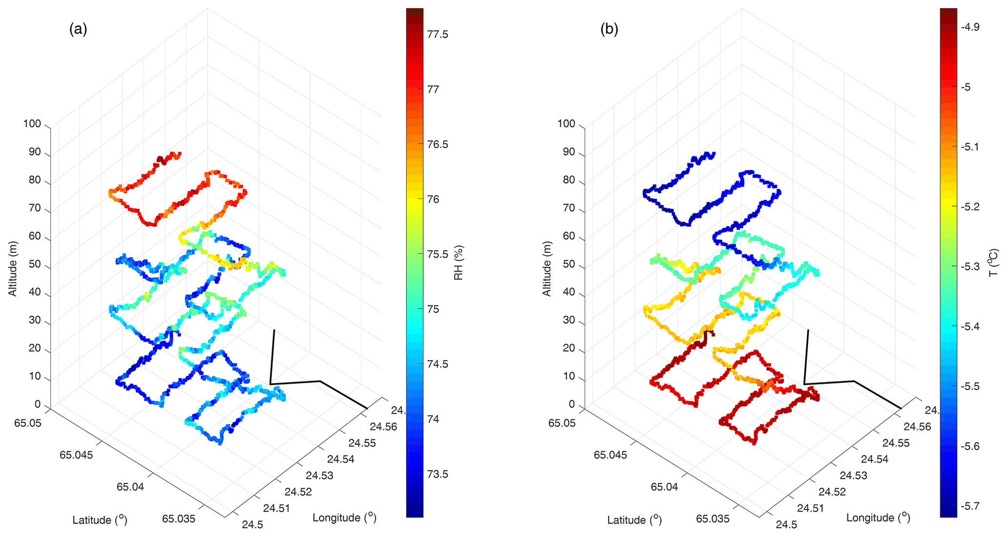
Figure 4UAV-UG1 measurements of (a) relative humidity and (b) air temperature from Flight 3.2 (Table 1). The black line indicates Hailuoto's Marjaniemi shoreline.
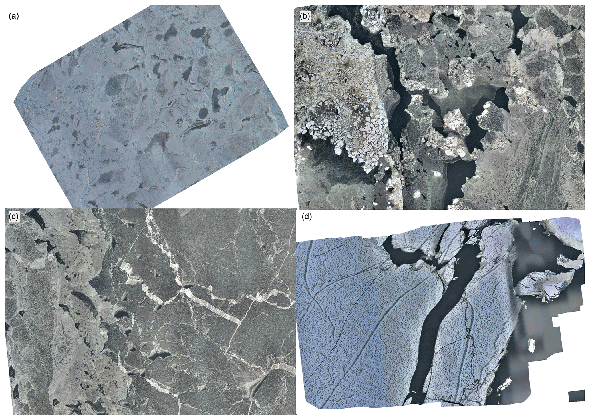
Figure 5Overview of the orthomosaic maps of the ice surface generated by stitching individual images from DJI Mavic 2 Pro photogrammetry missions: (a) first map from 27 February located ∼65 m to the south of Hailuoto's Marjaniemi pier; (Flight 0.1, magenta line in Fig. 1a); maps of the main survey area (Fig. 1b) from (b) 28 February, (c) 29 February, and (d) 1 March.
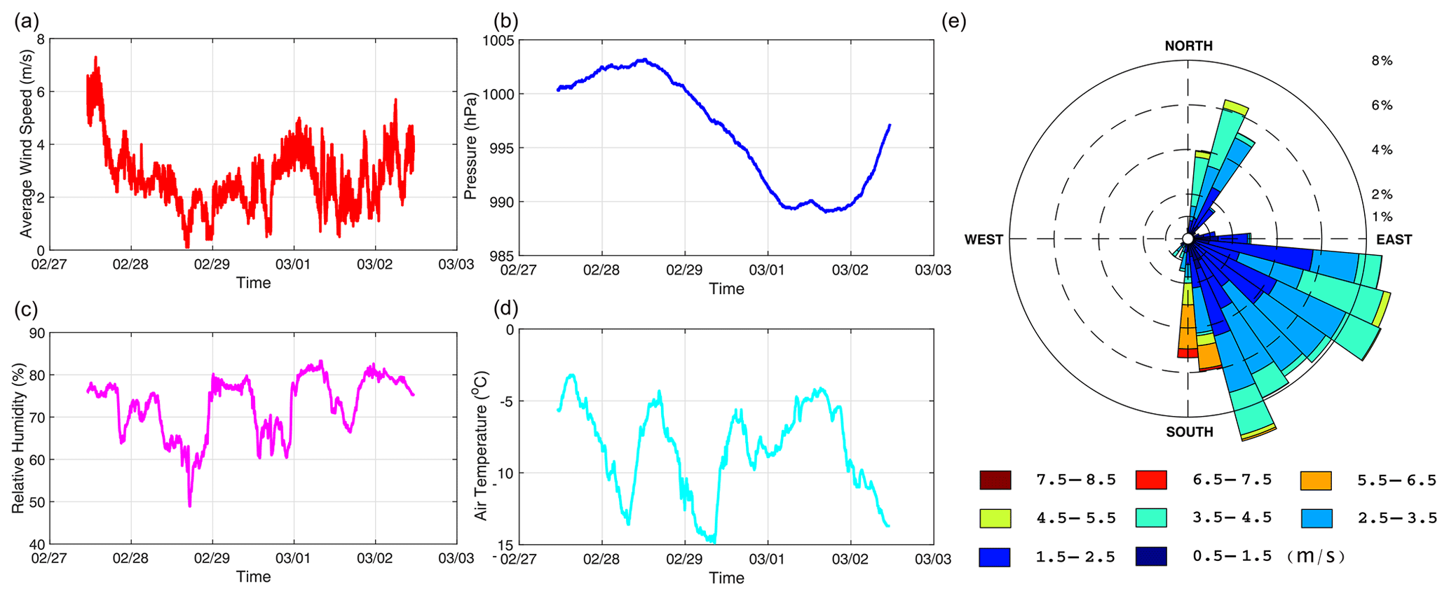
Figure 6Automatic weather station measurements during the HAOS campaign: time series of (a) wind speed, (b) atmospheric pressure, (c) relative humidity, and (d) air temperature and (e) statistics of wind direction and speed.

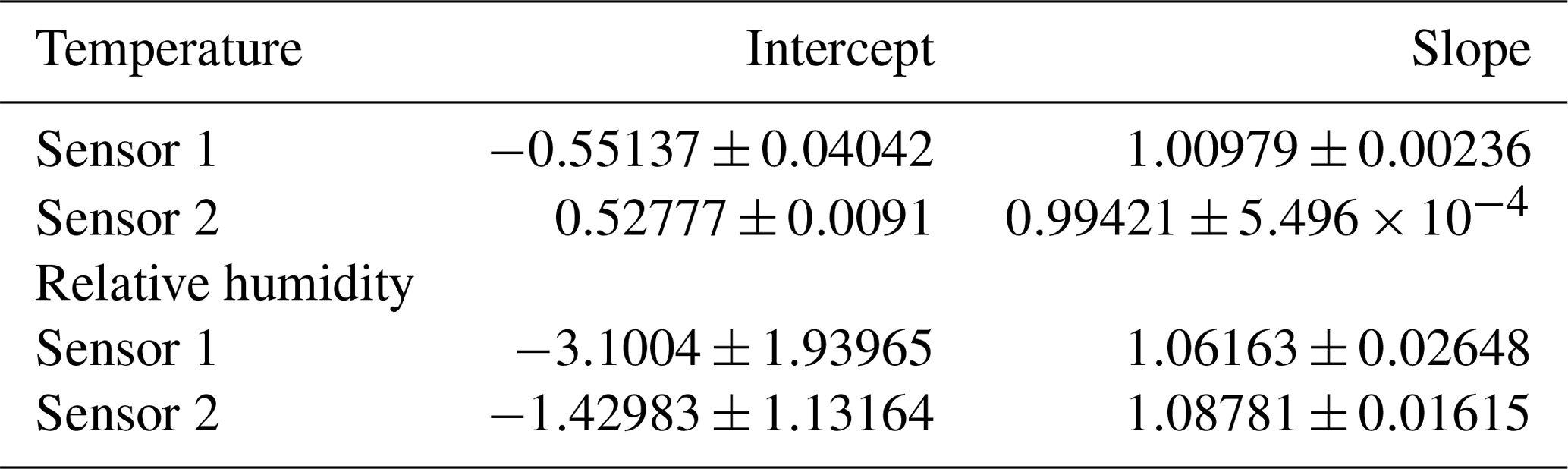
Table 3Intercept and slope coefficients for the calibration of UAV-UG1 and UAV-UG2 meteorological sensors.
3.1 Ground meteorological measurements
The ground meteorological observations were done by a 3D sonic anemometer (uSonic-3 Scientific, formerly USA-1, METEK GmbH) and an automatic weather station (WXT, Vaisala Inc.). Both instruments were mounted on a metal mast at a height of 2.5 m above the ground surface (Fig. 3d). The 3D anemometer measured three wind speed components (u, v, and w in m s−1) and acoustic temperature (T in ∘C) at 10 Hz resolution. The Vaisala WXT sensor measured the ambient temperature, relative humidity, rain intensity, wind direction, and wind speed. The following parameters were logged as 1 min averages: date and time (DD-MM-YY HH:MM), minimum wind direction (deg), averaged wind direction (deg), maximum wind direction (deg), minimum wind speed (m s−1), averaged wind speed (m s−1), maximum wind speed (m s−1), temperature (∘C), relative humidity (%), and pressure (hPa). A summary of the measured values is shown in Fig. 6.
3.2 Halo Doppler lidar
A Halo Photonics StreamLine XR scanning Doppler lidar (Pearson et al., 2009) was installed at the location of the weather station at a height of 1.3 m a.g.l. The StreamLine XR is capable of full hemispheric scanning, and the scanning patterns are fully user configurable. In the vertically pointing mode, the lidar alternates between co- and cross-polar receivers. The minimum range of the lidar is 90 m, and its instrumental specifications are given in Table 2.
During the campaign at Hailuoto, the scanning schedule included five scans in addition to the vertically pointing stare with alternating co- and cross-polar measurements. The scans were as follows: (1) a sector scan at 0∘ elevation angle, azimuth angle ranging from 180 to 360∘ at 5∘ steps; (2) a sector scan at 2∘ elevation angle, azimuth angle ranging from 180 to 360∘ at 10∘ steps; (3) a vertical azimuth display (VAD) scan at 10∘ elevation angle with 15∘ steps in azimuth angle; (4) a VAD scan at 70∘ elevation angle with 15∘ steps in azimuth angle; and (5) a vertically pointing co-polar scan repeated for 12 rays. The integration time for each scan type was set to 6 s. Sector scans and VADs (scans 1–4) were used to retrieve horizontal winds and a proxy for turbulence at different heights and ranges, similar to Vakkari et al. (2015). The last scan (5) was used to estimate the turbulent kinetic energy (TKE) dissipation rate according to O'Connor et al. (2010).
The measurements were post-processed according to Vakkari et al. (2019), and the attenuated backscatter (β) was calculated from signal-to-noise ratio (SNR) taking into account the telescope focus (infinity). The uncertainties in radial velocity and β were calculated according to O'Connor et al. (2010). The data were visually inspected, and range gate 14 was excluded from further analyses due to the increased noise floor. Both the original radial velocity data and the retrieved parameters, i.e., the horizontal wind speed and direction, TKE dissipation rate, and turbulence proxy (Vakkari et al., 2015), are stored in data files in netCDF format.
For each UAV-UG1 flight listed in Table 1, two files in the tab-delimited format are available with measurements from both meteorological sensors (Bosh BME280) (e.g., “Flight 1.01-sensor 1” and “Flight 1.01-sensor 2”) which collected data simultaneously during the flight. Each file includes the following variables following the format description (name in the file): geolocation data from GPS sensor: latitude (Latitude), longitude (Longitude), UTM coordinates (UTM east, UTM north), altitude (Altitude), date and time (Date/Time), date and time in serial date number format (Time), air pressure (PPPP), temperature (TTT), and relative humidity (RH). The altitude values, due to the high uncertainties in the GPS sensor output, were calculated from the atmospheric pressure P and temperature T measurements using the hypsometric equation:
where P0 denotes the surface pressure from the weather station. The initial and final flight segments outside of the target survey path were removed from the files, as described earlier in Sect. 2.3. Apart from this process, no data were rejected, and no missing values were found. Example measurements from Flight 3.2 are presented in Fig. 4. The UAV-UG1 and UAV-UG2 measurements of temperature and relative humidity over the survey area are provided without calibration – as they were measured. The calibrated values of the temperature and relative humidity from both UAV-UG2 sensors can be obtained with a linear calibration equation, with intercept (a) and slope (b) coefficients from Table 3. All correlation coefficients (Pearson's R, R square and adjusted R square) are higher than 0.997. Due to the sensors' exposure to sunlight dependent on the relative orientation of the aircraft and the sun (different during different fragments of the survey path and changing throughout the day), measurements from the sensor with lower air temperature are recommended for further analysis.
The orthomosaic maps (Fig. 5) of the surface below UAV-UG1 flight paths are available in GeoTIFF and KML formats.
The Halo Doppler lidar dataset consists of seven netCDF files per day for each day between 28 February and 2 March 2020. Each file name begins with the prefix “YYYYmmdd” indicating the day of the measurements and an affix related to file contents: (1) co-polar and (2) cross-polar background measurements (co.nc and cross.nc) and (3) TKE dissipation rate retrieved from the measurements (TKE.nc) and four VAD scans of horizontal wind speed and direction with the elevation angles of (4) 0∘ (VAD0-wind.nc), (5) 2∘ (VAD2-wind.nc), (6) 10∘ (VAD10-wind.nc), and (7) 70∘ (VAD70-wind.nc). A detailed description of Halo Doppler lidar measurement post-processing can be found in Sect. 3.2.
The automatic weather station measurements are provided in the tab-delimited format with a separate file for each day of the campaign. The files, labeled with the prefix “aws” for automatic weather station and the relevant date, include all the variables listed in Sect. 2.3. The 3D anemometer measurements conducted at the same location are provided in raw, hourly generated, tab-delimited files with the following variables: time in the “HHMMSS.ss” (hours, minutes, seconds, milliseconds) format, the three wind speed components u, v, and w (), and acoustic temperature Ts ().
All the described datasets are available to the public in the described formats at https://doi.org/10.1594/PANGAEA.918823 (Wenta et al., 2020). The repository is hosted by the Alfred Wegener Institute, Helmholtz Center for Polar and Marine Research (AWI), and the Center for Marine Environmental Sciences, University of Bremen (MARUM).
During the HAOS campaign between 27 February and 2 March 2020, 27 fixed-wing UAV-UG1 flights were carried out off the shore of the westernmost point of Hailuoto island, together with overlapping photogrammetry missions, which resulted in four orthomosaic maps of the sea ice below. Additionally, a 3D sonic anemometer, automatic weather station, and Halo Doppler lidar operated near Hailuoto's Marjaniemi lighthouse throughout the time of the HAOS project.
The primary focus of HAOS was to obtain detailed measurements of the atmospheric boundary layer over sea ice. In accordance with this goal, sUAV flights provided continuous 3D meteorological observations over sea ice offshore and were supplemented by onshore measurements of atmospheric state. Thus, the presented dataset provides a thorough description of the atmospheric conditions over newly formed sea ice near Hailuoto island. Furthermore, detailed orthomosaic maps provide a unique and extremely detailed view of the newly formed sea ice and its changes in the span of 4 d (Fig. 5). Considering the scarcity of recent ABL observations over diminishing sea ice cover in the Bay of Bothnia, and the Baltic Sea in general, the presented dataset may be considered as a valuable source of information and the basis for further studies on sea ice–atmospheric interactions in this region. Additionally, as the weather conditions throughout the campaign resembled the ones observed over sea ice in the Arctic, the HAOS dataset can also be used in the studies related to polar regions.
DB and KD designed, constructed, and configured the drones. VV was responsible for the lidar measurements. MW and AH planned the research. All authors contributed to the conduction of measurements and data processing and discussed the results. MW, DB, and VV wrote the paper.
The authors declare that they have no conflict of interest.
This work was funded by the Polish National Science Centre grant no. 2018/31/B/ST10/00195 “Observations and modeling of sea ice interactions with the atmospheric and oceanic boundary layers”.
This paper was edited by Ge Peng and reviewed by two anonymous referees.
Batrak, J. and Müller, M.: Atmospheric Response to Kilometer-Scale Changes in Sea Ice Concentration Within the Marginal Ice Zone, Geophys. Res. Lett., 45, 6702–6709, https://doi.org/10.1029/2018GL078295, 2018. a
Bhardwaj, A., Sam, L., Martìn-Torres, A. J., and Kumar, R.: UAVs as remote sensing platform in glaciology: Present applications and future prospects, Remote Sens. Environ., 175, 196–204, https://doi.org/10.1016/j.rse.2015.12.029, 2016. a
Brümmer, B.: Roll and Cell Convection in Wintertime Arctic Cold-Air Outbreaks, J. Atmos. Sci., 56, 2613–2636, https://doi.org/10.1175/1520-0469(1999)056<2613:RACCIW>2.0.CO;2, 1999. a
Cassano, J. J., Seefeldt, M. W., Palo, S., Knuth, S. L., Bradley, A. C., Herrman, P. D., Kernebone, P. A., and Logan, N. J.: Observations of the atmosphere and surface state over Terra Nova Bay, Antarctica, using unmanned aerial systems, Earth Syst. Sci. Data, 8, 115–126, https://doi.org/10.5194/essd-8-115-2016, 2016. a
deBoer, G., Ivey, M., Schmid, B., Lawrence, D., Dexheimer, D., Mei, F., Hubbe, J., Bendure, A., Hardesty, J., Shupe, M., McComiskey, A., Telg, H., Schmitt, C., Matrosov, S., Brooks, I., Creamean, J., Solomon, A., Turner, D., Williams, C., Maahn, M., Argrow, B., Palo, S., Long, C., Gao, R., and Mather, J.: A Bird's-Eye View: Development of an Operational ARM Unmanned Aerial Capability for Atmospheric Research in Arctic Alaska, B. Am. Meteorol. Soc., 99, 1197–1212, https://doi.org/10.1175/BAMS-D-17-0156.1, 2018. a
Frech, M. and Jochum, A.: The Evaluation of Flux Aggregation Methods using Aircraft Measurements in the Surface Layer, Agr. Forest Meteorol., 98-9, 121–143, https://doi.org/10.1016/S0168-1923(99)00093-3, 1999. a
Gaffey, C. and Bhardwaj, A.: Applications of Unmanned Aerial Vehicles in Cryosphere: Latest Advances and Prospects, Remote Sens., 12, 948, https://doi.org/10.3390/rs12060948, 2020. a
Horvat, C. and Tziperman, E.: A prognostic model of the sea-ice floe size and thickness distribution, The Cryosphere, 9, 2119–2134, https://doi.org/10.5194/tc-9-2119-2015, 2015. a
Knuth, S. L., Cassano, J. J., Maslanik, J. A., Herrmann, P. D., Kernebone, P. A., Crocker, R. I., and Logan, N. J.: Unmanned aircraft system measurements of the atmospheric boundary layer over Terra Nova Bay, Antarctica, Earth Syst. Sci. Data, 5, 57–69, https://doi.org/10.5194/essd-5-57-2013, 2013. a
Kral, S., Reuder, J., Vihma, T., Suomi, I., O'Connor, E., Kouznetsov, R., Wrenger, B., Rautenberg, A., Urbancic, G., Jonassen, M., Båserud, J., Maronga, B., Mayer, S., Lorenz, T., Holtslag, A., Steeneveld, G., Seidl, A., Müller, M., Lindenberg, C., and Schygulla, M.: Innovative Strategies for Observations in the Arctic Atmospheric Boundary Layer (ISOBAR) – The Hailuoto 2017 Campaign, Atmosphere, 9, 268, https://doi.org/10.3390/atmos9070268, 2018. a
Kral, S., Reuder, J., Vihma, T., Suomi, I., Haualand, K., Urbancic, G., Greene, B., Steeneveld, G., Lorenz, T., Maronga, B., Jonassen, M., Ajosenpå, H., Bæserud, L., Chilson, P., Holtslag, A., Jenkins, A., Kouznetsov, R., Mayer, S., Pillar-Little, E., Rautenberg, A., Schwenkel, J., Seidl, A., and Wrenger, B.: The Innovative Strategies for Observations in the Arctic Atmospheric Boundary Layer Project (ISOBAR) – Unique fine-scale observations under stable and very stable conditions, B. Am. Meteorol. Soc., 1–64, https://doi.org/10.1175/BAMS-D-19-0212.1, 2020. a
LeadEx Group: The LeadEx experiment, EOS. Trans. AGU, 74, 393–397, https://doi.org/10.1029/93EO00341, 1993. a
Manucharyan, G. and Thompson, A.: Submesoscale Sea Ice-Ocean Interactions in Marginal Ice Zones, J. Geophys. Res.-Oceans, 122, 9455–9475, https://doi.org/10.1002/2017JC012895, 2017. a
O'Connor, E., Illingworth, A., Brooks, I., Westbrook, C., Hogan, R., Davies, G., and Brooks, B.: A Method for Estimating the Turbulent Kinetic Energy Dissipation Rate from a Vertically Pointing Doppler Lidar, and Independent Evaluation from Balloon-Borne In Situ Measurements, J. Atmos. Ocean. Tech., 27, 1652–1664, https://doi.org/10.1175/2010JTECHA1455.1, 2010. a, b
Pearson, G., Davies, F., and Collier, C.: An Analysis of the Performance of the UFAM Pulsed Doppler Lidar for Observing the Boundary Layer, J. Atmos. Ocean. Tech., 26, 240–250, https://doi.org/10.1175/2008JTECHA1128.1, 2009. a
Qu, M., Pang, X., Zhao, X., Zhang, J., Ji, Q., and Fan, P.: Estimation of turbulent heat flux over leads using satellite thermal images, The Cryosphere, 13, 1565–1582, https://doi.org/10.5194/tc-13-1565-2019, 2019. a
Tetzlaff, A., Lüpkes, C., and Hartmann, J.: Aircraft-based observations of atmospheric boundary-layer modification over Arctic leads, Q. J. Roy. Meteor. Soc., 141, 2839–2856, https://doi.org/10.1002/qj.2568, 2015. a
Uttal, T., Curry, J., Mcphee, M., Perovich, D., Moritz, R., Maslanik, J., Guest, P., Stern, H., Moore, J., Turenne, R., Heiberg, A., Serreze, M., Wylie, D., Persson, O., Paulson, C., Halle, C., Morison, J., Wheeler, P., Makshtas, A., Welch, H., Shupe, M., Intrieri, J., Stamnes, K., Lindsey, R., Pinkel, R., Pegau, W., Stanton, T., and Grenfeld, T.: Surface Heat Budget of the Arctic Ocean, B. Am. Meteorol. Soc., 83, 255–275, https://doi.org/10.1175/1520-0477(2002)083<0255:SHBOTA>2.3.CO;2, 2002. a
Vakkari, V., O'Connor, E. J., Nisantzi, A., Mamouri, R. E., and Hadjimitsis, D. G.: Low-level mixing height detection in coastal locations with a scanning Doppler lidar, Atmos. Meas. Tech., 8, 1875–1885, https://doi.org/10.5194/amt-8-1875-2015, 2015. a, b
Vakkari, V., Manninen, A. J., O'Connor, E. J., Schween, J. H., van Zyl, P. G., and Marinou, E.: A novel post-processing algorithm for Halo Doppler lidars, Atmos. Meas. Tech., 12, 839–852, https://doi.org/10.5194/amt-12-839-2019, 2019. a
Vihma, T., Pirazzini, R., Fer, I., Renfrew, I. A., Sedlar, J., Tjernström, M., Lüpkes, C., Nygård, T., Notz, D., Weiss, J., Marsan, D., Cheng, B., Birnbaum, G., Gerland, S., Chechin, D., and Gascard, J. C.: Advances in understanding and parameterization of small-scale physical processes in the marine Arctic climate system: a review, Atmos. Chem. Phys., 14, 9403–9450, https://doi.org/10.5194/acp-14-9403-2014, 2014. a, b
Wenta, M. and Herman, A.: The influence of the spatial distribution of leads and ice floes on the atmospheric boundary layer over fragmented sea ice, Ann. Glaciol., 59, 213–230, https://doi.org/10.1017/aog.2018.15, 2018. a
Wenta, M. and Herman, A.: Area-Averaged Surface Moisture Flux over Fragmented Sea Ice: Floe Size Distribution Effects and the Associated Convection Structure within the Atmospheric Boundary Layer, Atmosphere, 10, 654, https://doi.org/10.3390/atmos10110654, 2019. a
Wenta, M., Brus, D., Doulgeris, K.-M., Vakkari, V., and Herman, A.: Winter atmospheric boundary layer observations over sea ice in the coastal zone of the Bothnian Bay (Baltic Sea), PANGAEA, https://doi.org/10.1594/PANGAEA.918823, 2020. a, b
Zaugg, E., Edwards, M., Gomola, J., and Long, D.: SAR imaging of Arctic Sea Ice from an unmanned aircraft as part of the MIZOPEX project, 2013 IEEE Radar Conference (RadarCon13), Ottawa, ON, 1–5, https://doi.org/10.1109/RADAR.2013.6586016, 2013. a
Zhang, Y., Cheng, X., Liu, J., and Hui, F.: The potential of sea ice leads as a predictor for summer Arctic sea ice extent, The Cryosphere, 12, 3747–3757, https://doi.org/10.5194/tc-12-3747-2018, 2018. a