Status of the Tibetan Plateau observatory (Tibet-Obs) and a 10-year (2009–2019) surface soil moisture dataset

The Tibetan Plateau observatory (Tibet-Obs) of plateau scale soil moisture and soil temperature was established 10 years ago and has been widely used to calibrate/validate satellite- and model-based soil moisture (SM) products for their applications to the Tibetan Plateau (TP). This paper reports on the status of the Tibet-Obs and presents a 10-year (2009–2019) surface SM dataset produced based on in situ measurements taken at a depth of 5 cm collected from the Tibet-Obs that consists of three regional-scale SM monitoring networks, i.e. the Maqu, Naqu, and Ngari (including Ali and Shiquanhe) networks. This surface SM dataset includes the original 15 min in situ measurements collected by multiple SM monitoring sites of the three networks and the spatially upscaled SM records produced for the Maqu and Shiquanhe networks. Comparisons between four spatial upscaling methods – i.e. arithmetic averaging, Voronoi diagrams, time stability, and apparent thermal inertia – show that the arithmetic average of the monitoring sites with long-term (i.e. ≥ 6-year) continuous measurements is found to be most suitable to produce the upscaled SM records. Trend analysis of the 10-year upscaled SM records indicates that the Shiquanhe network in the western part of the TP is getting wet, while there is no significant trend found for the Maqu network in the east. To further demonstrate the uniqueness of the upscaled SM records in validating existing SM products for a long-term period (∼10 years), the reliability of three reanalysis datasets is evaluated for the Maqu and Shiquanhe networks. It is found that current model-based SM products still show deficiencies in representing the measured SM dynamics in the Tibetan grassland (i.e. Maqu) and desert ecosystems (i.e. Shiquanhe). The dataset would also be valuable for calibrating/validating long-term satellite-based SM products, evaluation of SM upscaling methods, development of data fusion methods, and quantifying the coupling of SM and precipitation at a 10-year scale. The dataset is available in the 4TU.ResearchData repository at https://doi.org/10.4121/12763700.v7 (Zhang et al., 2020).

1 Introduction

The Tibetan Plateau observatory (Tibet-Obs) of plateau scale soil moisture and soil temperature (SMST) was set up in 2006 and became fully operational in 2010 with the objective of calibration/validation of satellite- and model-based soil moisture (SM) products at a regional scale (Su et al., 2011). The Tibet-Obs mainly consists of three regional-scale SMST monitoring networks – i.e. Maqu, Naqu, and Ngari – which cover different climate and land surface conditions across the Tibetan Plateau (TP), and each includes multiple in situ SMST monitoring sites. The SM data collected from the Tibet-Obs have been widely used in the past decade to calibrate/validate satellite- and model-based SM products (e.g. Su et al., 2013; Zheng et al., 2015a, b; Colliander et al., 2017), to evaluate and develop SM upscaling methods (e.g. Qin et al., 2013, 2015), to assess algorithms for the retrieval of SM for microwave remote sensing observations (e.g. van der Velde et al., 2014a, b; Zheng et al., 2018a, b, 2019), and to assess fusion methods for merging in situ SM and satellite- or model-based products (e.g. Yang et al., 2020; Zeng et al., 2016).

Table 1 Summary of the main Tibet-Obs applications and corresponding findings.

Key information and outcomes of the main scientific applications using the Tibet-Obs SM data are summarized in Table 1. As shown in Table 1, the state-of-the-art satellite- and model-based products are useful but still show various types of deficiencies specific to the hydro-meteorological conditions on the TP, and further evaluation and improvement of these products remain imperative. In general, previous studies mainly focused on the evaluation of SM products using the Tibet-Obs data for short-term periods (i.e. less than 5 years), while up to now the Tibet-Obs has collected in situ measurements for more than 10 years. Development of a close-to-10-year Tibet-Obs in situ SM dataset will further enhance the calibration/validation of long-term satellite- and model-based products and is valuable for better understanding the hydro-meteorological response to climate change. However, SM is highly variable in both space and time, and data gaps in the availability of measurements taken from individual monitoring sites hinder scientific studies covering longer time periods, e.g. more than 5 years. Therefore, it is still challenging to obtain accurate long-term regional-scale SM due to the sparse nature of monitoring networks and highly variable soil conditions.

Spatial upscaling is usually necessary to obtain the regional-scale SM of an in situ network from multiple monitoring sites to match the footprint of satellite- or the grid cell of model-based products. A frequently used approach for upscaling point-scale SM measurements to a spatial domain is the arithmetic average, mostly because of its simplicity (Su et al., 2011, 2013). Many other studies also adopted weighted averaging methods, whereby the weights are assigned to account for spatial heterogeneity in the area covered by in situ monitoring sites within the network. For instance, Colliander et al. (2017) employed Voronoi diagrams to determine the weights of individual monitoring sites within core regional-scale networks used for the worldwide validation of the Soil Moisture Active Passive (SMAP) SM products. Dente et al. (2012b) established weights based on the topography and soil texture for the sites of the Tibet-Obs's Maqu network. Qin et al. (2013, 2015) derived the weights by minimizing a cost function between in situ SM of individual monitoring sites and a representative SM of the network that is estimated using the apparent thermal inertia (ATI)-based method (Gao et al., 2017). Alternative methods, such as time stability and ridge regression, have been adopted in other investigations (i.e. Zhao et al., 2013; Kang et al., 2017). While a large number of studies have assessed the performance of different upscaling methods in other areas such as the Tonzi Ranch network in California and the Heihe watershed (Moghaddam et al., 2014; Wang et al., 2014), only a few investigations have been done for the TP (Gao et al., 2017; Qin et al., 2015). Since the number of monitoring sites changes over time due to damage to SM sensors in the Tibet-Obs, it is essential to evaluate and select an appropriate upscaling method for a limited number of monitoring sites (i.e. ≤ four sites).

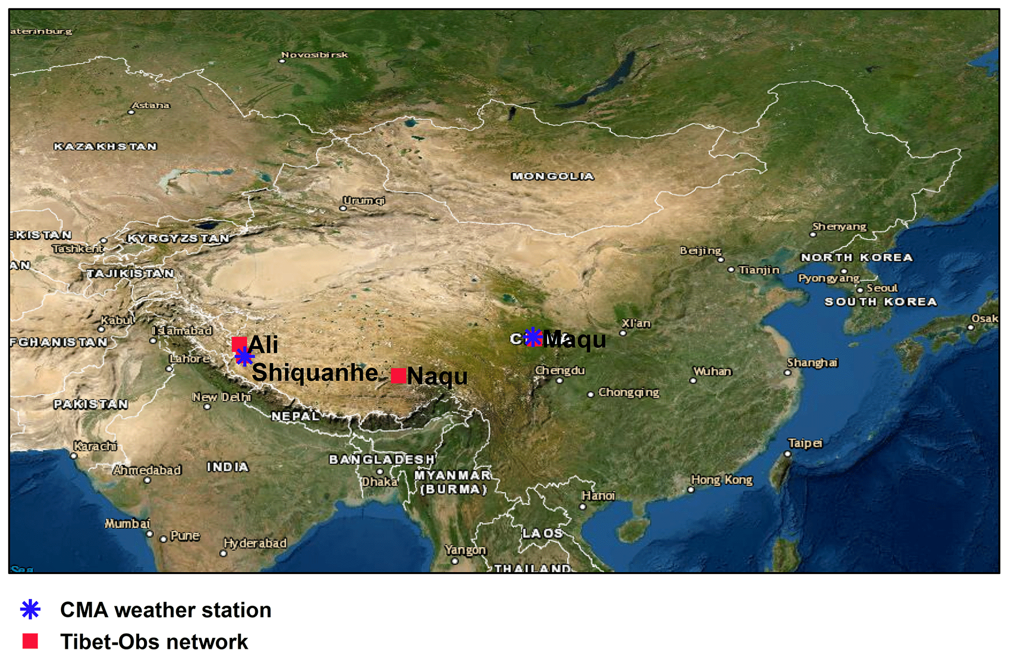
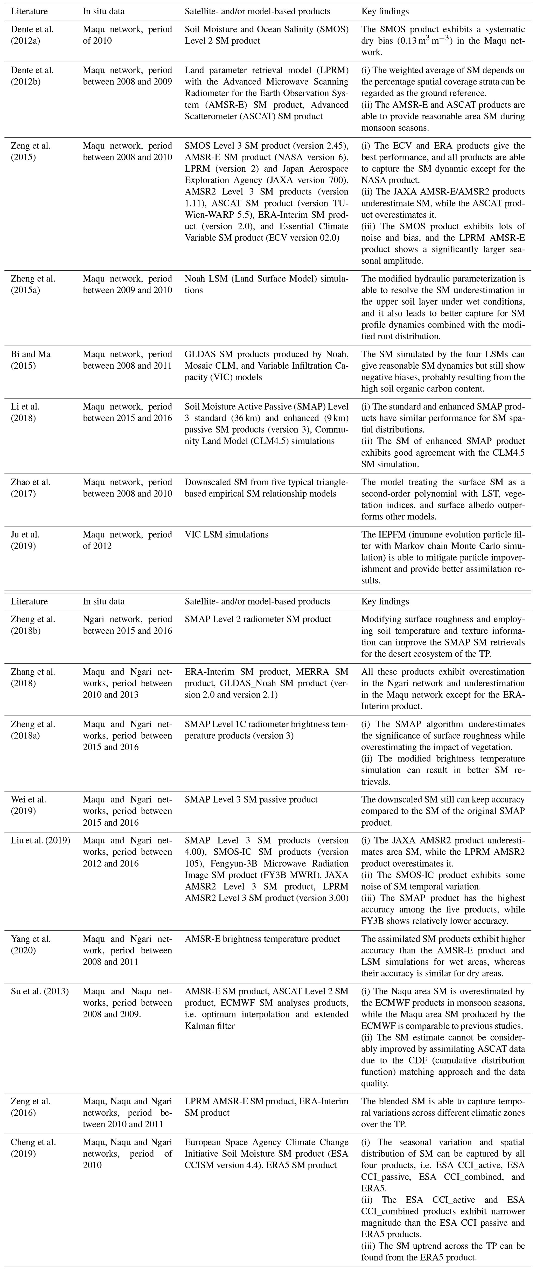
Figure 1 Locations of the Tibet-Obs including Maqu, Naqu, and Ngari (including Ali and Shiquanhe) soil moisture monitoring networks. The weather stations of Maqu and Shiquanhe operated by the China Meteorological Administration (CMA) are also shown. (Base map is from Esri, Copyright: © Esri.)

This paper reports on the status of the Tibet-Obs and presents a long-term in situ SM and spatially upscaled SM dataset for the period between 2009 and 2019. The 10-year SM dataset of Tibet-Obs includes the original 15 min in situ measurements taken at a depth of 5 cm collected from the three regional-scale networks (i.e. Maqu, Naqu, and Ngari as shown in Fig. 1) and the continuous regional-scale SM produced using an appropriately selected spatial upscaling method. To achieve this, four methods are studied, namely the arithmetic average (AA), Voronoi diagram (VD), time stability (TS), and apparent thermal inertia (ATI) methods. The seasonal dynamic and trend of the regional-scale SM time series are analysed, and the 10-year SM dataset is used to validate three model-based SM products, i.e. ERA5-Land (Muñoz-Sabater et al., 2018), MERRA2 (Modern-Era Retrospective Analysis for Research and Applications version 2) (GMAO, 2015), and GLDAS Noah (Global Land Data Assimilation System with Noah Land Surface Model) (Rodell et al., 2004).

This paper is organized as follows. Section 2 describes the status of the Tibet-Obs and the in situ SM measurements, as well as the precipitation data and the three model-based SM products. Section 3 introduces the four SM spatial upscaling methods, the Mann–Kendall trend test and Sen's slope estimate, and performance metrics. Section 4 presents the inter-comparison of the four SM spatial upscaling methods, the production and analysis of the regional-scale SM dataset for a 10-year period, and its application to validate the three model-based SM products. Section 5 provides the discussion and suggestions for maintaining Tibet-Obs. Section 6 documents the information on data availability, and the conclusions are drawn in Sect. 7.

2 Data

2.1 Status of the Tibet-Obs

The Tibet-Obs consists of the Maqu, Naqu, and Ngari (including Shiquanhe and Ali) regional-scale SMST monitoring networks (Fig. 1), which cover a cold humid climate, cold semi-arid climate, and cold arid climate, respectively. Each network includes a number of monitoring sites that measure the SMST at different soil depths. Brief descriptions of each network and corresponding surface SM measurements taken at a depth of 5 cm are given in the following subsections. The readers are referred to the existing literature (Su et al., 2011; Dente et al., 2012b; Zhao et al., 2018) for additional information on the networks.

2.1.1 Maqu network

The Maqu network is located in the north-eastern edge of the TP ($\mathrm{33}{}^{\circ }{\mathrm{30}}^{\prime }$–$\mathrm{34}{}^{\circ }{\mathrm{15}}^{\prime }$ N, $\mathrm{101}{}^{\circ }{\mathrm{38}}^{\prime }$–$\mathrm{102}{}^{\circ }{\mathrm{45}}^{\prime }$ E) at the first major bend of the Yellow River. The landscape is dominated by the short grass at elevations varying from 3400 to 3800 m. The climate type is characterized as cold and humid with cold dry winters and rainy summers. The mean annual air temperature is about 1.2 ^∘C, with −10 ^∘C for the coldest month (January) and 11.7 ^∘C for the warmest month (July) (Zheng et al., 2015a). The annual precipitation is about 600 mm, which falls mainly in the warm season (May–October).

The Maqu network covers an area of approximately 40 km by 80 km and originally consisted of 20 SMST monitoring sites installed in 2008 (Dente et al., 2012b). During the period between 2014 and 2016, eight new sites were installed due to the damage to several old monitoring sites caused by local people or animals. The basic information of each monitoring site is summarized in Table A1 (Su et al., 2011), and the typical characteristics of topography and land cover within the network are shown in Fig. 2 as well.

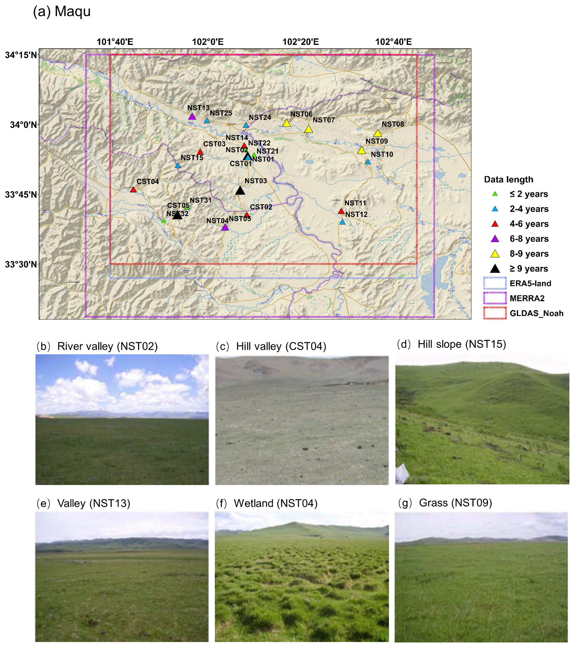
Figure 2 (a) Overview of the Maqu monitoring network, and typical characteristics of topography and land cover within the network: (b) river valley, (c) hill valley, (d) hill slope, (e) valley, (f) wetland, and (g) grass. The coloured triangles in panel (a) represent different data lengths of surface SM measurements for each site, and the coloured boxes represent the coverage of selected model-based products. The site name in brackets in panels (b–g) indicates the site location for which the photograph is selected. (Base map copyright: © 2018 Garmin.)

Figure 3 Examples of typical installation of sensors in monitoring sites of (a) Maqu and (b) Ngari networks.

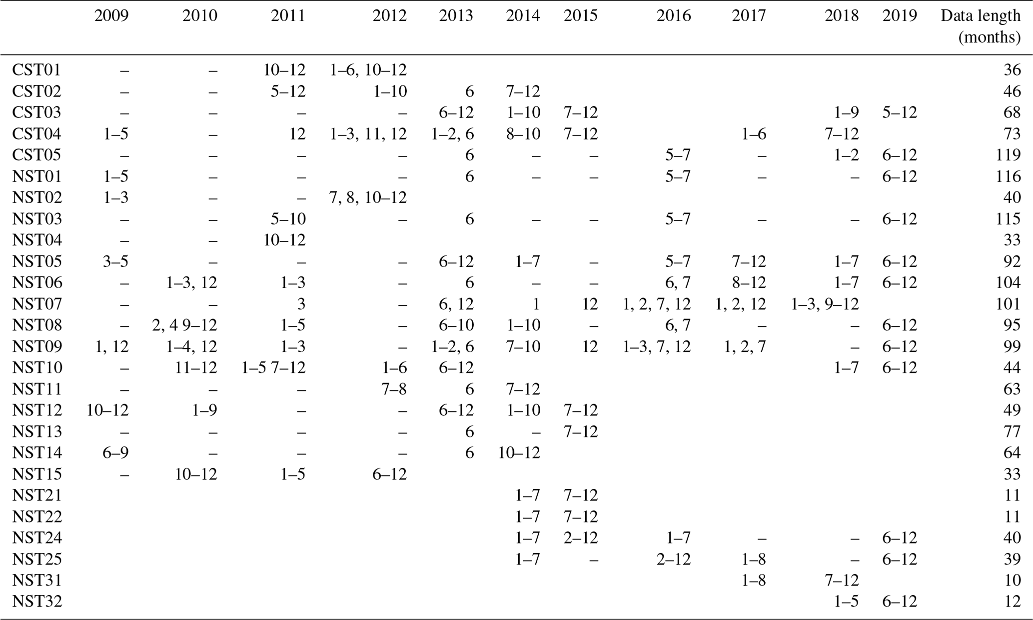
The Decagon 5TM ECH₂O probes are used to measure the SMST at nominal depths of 5, 10, 20, 40, and 80 cm (Fig. 3). The 5TM probe is a capacitance sensor measuring the dielectric permittivity of soil, and the Topp equation (Topp et al., 1980) is used to convert the dielectric permittivity to the volumetric SM. The accuracy of the 5TM volumetric SM was improved via a soil-specific calibration performed under laboratory conditions for each soil type found in the Maqu area (Dente et al., 2012b), leading to a decrease in the root mean square error (RMSE) from 0.06 to 0.02 m³ m⁻³ (Dente et al., 2012b). Table 2 provides the specific periods of data missing during each year and the total data lengths of surface SM for each monitoring site. Among these sites, the CST05, NST01, and NST03 have collected more than 9 years of SM measurements, while the data records for the NST21, NST22, and NST31 are less than 1 year. In May 2019, there were still 12 sites that provided SM data.

Table 2 Data records of all the SMST monitoring sites performed for the Maqu network. Blank cells represent that there are no measurements performed. Cells with a hyphen represent that data are available. The number in cells represents the month(s) when the data are missing during a year.

2.1.2 Ngari network

The Ngari network is located in the western part of the TP at the headwater of the Indus River. It consists of two SMST networks established around the cities of Ali and Shiquanhe. The landscape is dominated by a desert ecosystem at elevations varying from 4200 to 4700 m. The climate is characterized as cold and arid with a mean annual air temperature of 7.0 ^∘C. The annual precipitation is less than 100 mm, which falls mainly in the monsoon season (July–August) (van der Velde et al., 2014b).

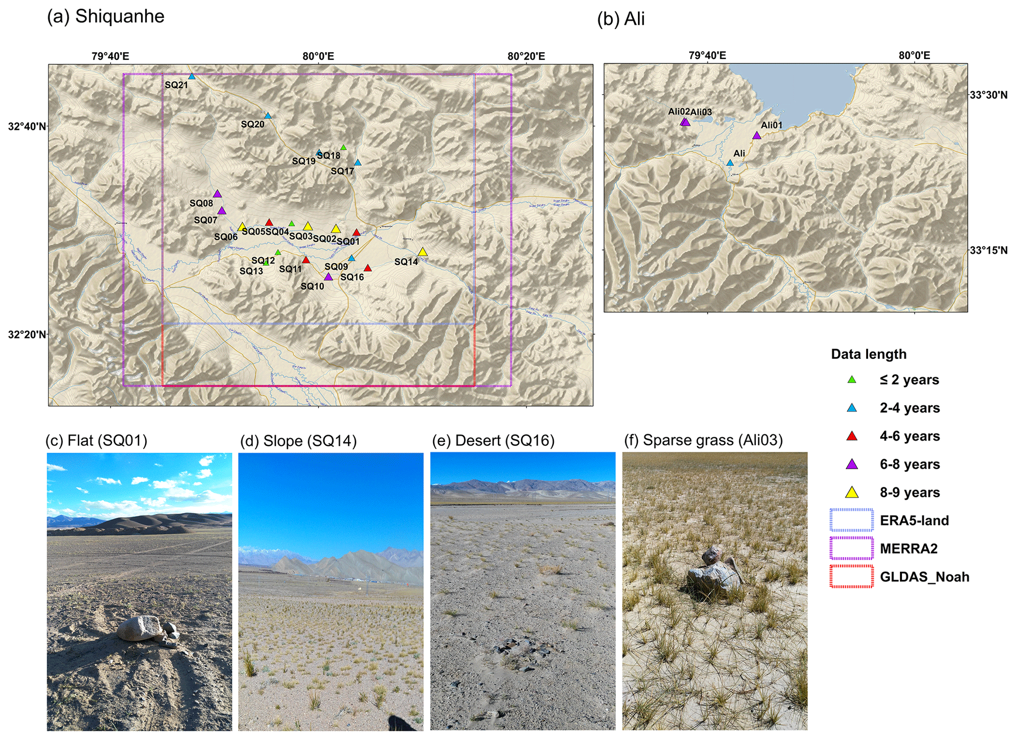
Figure 4 Overview of the Ngari monitoring network including (a) Shiquanhe and (b) Ali networks, and typical characteristics of topography and land cover within the network: (c) flat, (d) slope, (e) desert, and (f) sparse grass. The coloured triangles in panels (a, b) represent different data lengths of surface SM measurements for each site, and the coloured boxes represent the coverage of selected model-based products. The site name in brackets in panels (c–f) indicates the site location for which the photograph is selected. (Base map copyright: © 2018 Garmin.)

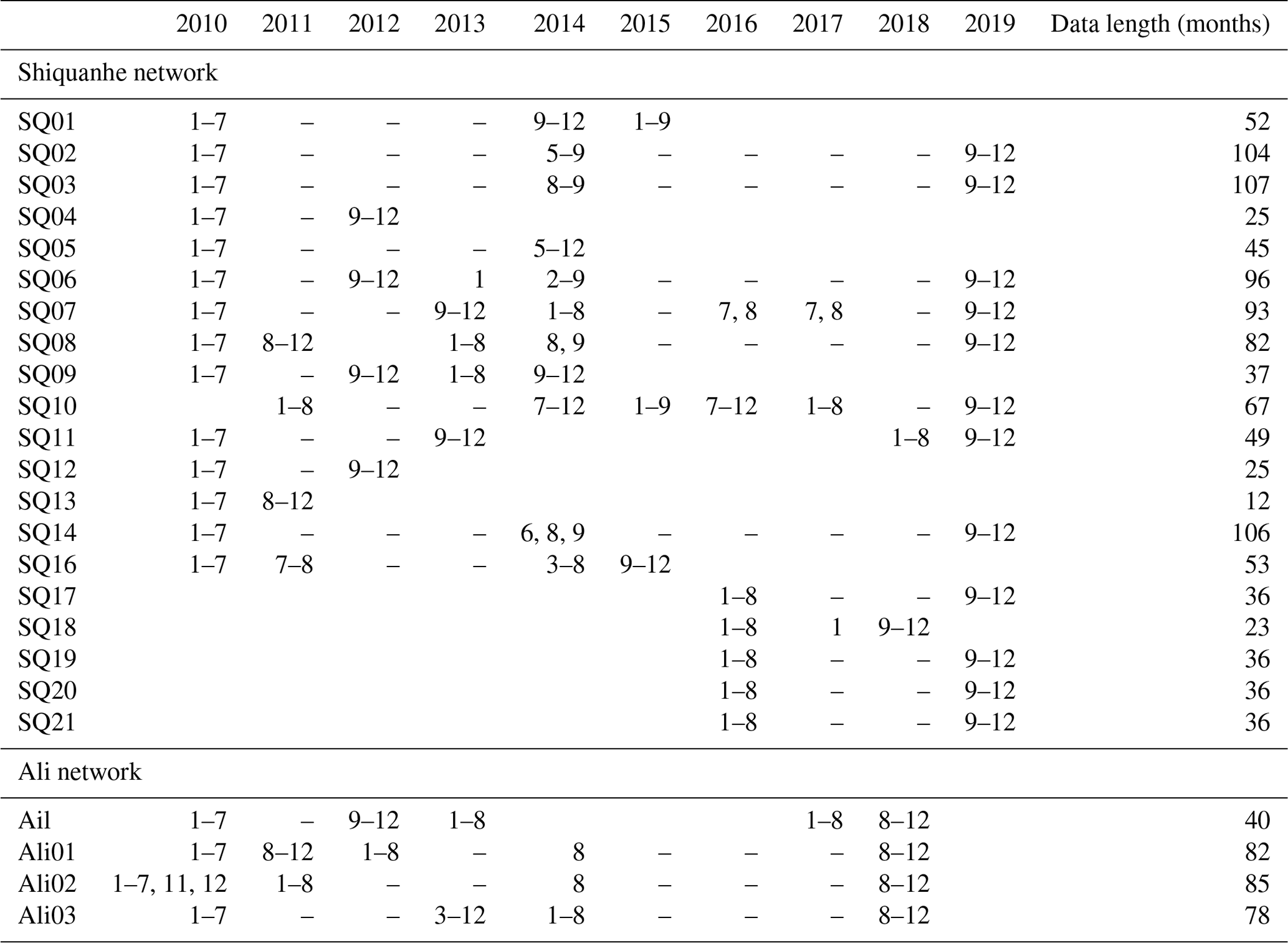
The Shiquanhe network originally consisted of 16 SMST monitoring sites installed in 2010 (Su et al., 2011), and five new sites were installed in 2016. The basic information of each monitoring site is summarized in Table A3 (Su et al., 2011), and the typical characteristics of topography and land cover within the network are also shown in Fig. 4. The Decagon 5TM ECH₂O probes were installed at depths of 5, 10, 20, 40, and 60 or 80 cm to measure the SMST (Fig. 3). Table 3 provides the specific periods of data missing during each year and the total data lengths of surface SM for each site. Among these sites, the SQ02, SQ03, SQ06, and SQ14 have collected more than 8 years of SM measurements, while the data records for the SQ13, SQ15, and SQ18 are less than 2 years. In August 2019, there were still 12 sites that provided SM data. The Ali network comprises four SM monitoring sites (Table A3), which will not be used for further analysis in this study due to limited number of monitoring sites and the availability of data records (Table 3).

Table 3 Same as Table 2 but for the Ngari network.

2.1.3 Naqu network

The Naqu network is located in the Naqu River basin with an average elevation of 4500 m. The climate is characterized as cold and semi-arid with cold dry winters and rainy summers. Over three-quarters of the total annual precipitation sum (400 mm) falls between June and August (Su et al., 2011). The landscape is dominated by short grass.

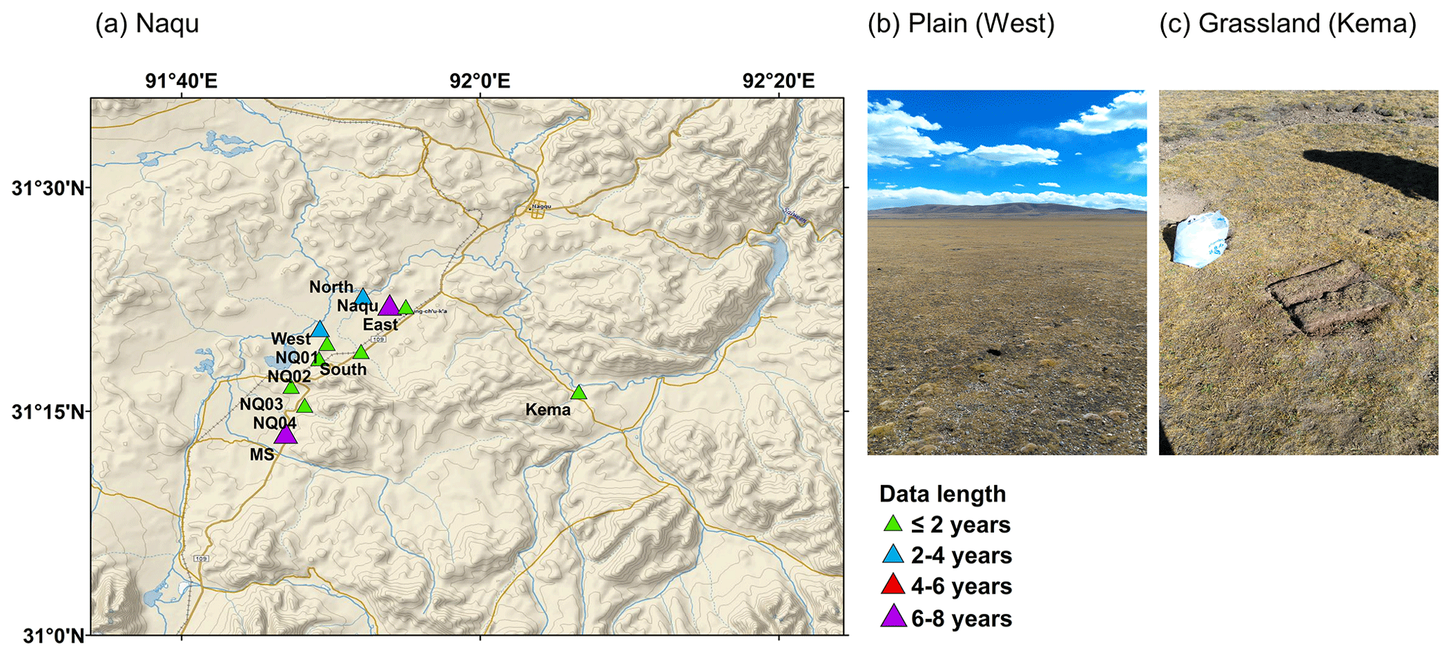
Figure 5 (a) Overview of the Naqu monitoring network, and typical characteristics of topography and land cover within the network: (b) plain and (c) grassland. The coloured triangles in panel (a) represent different data lengths of surface SM measurements for each site. The site name in brackets in panels (b, c) indicates the site location for which the photograph is selected. (Base map copyright: © 2018 Garmin.)

The network originally consisted of five SMST monitoring sites installed in 2006 (Su et al., 2011), and six new sites were installed between 2010 and 2016. The basic information of each monitoring site is summarized in Table A5, and the typical topography and land cover within the network are shown in Fig. 5 as well. The Decagon 5TM ECH₂O probes were installed at depths of 5 or 2.5, 10 or 7.5, 15, 30, and 60 cm to measure the SMST, and an on-site soil-specific calibration is reported in van der Velde (2010) and yielded a RMSE of 0.029 m³ m⁻³. Table 4 provides the specific periods of data missing during each year and the total data lengths of surface SM for each site. Among these sites, only two sites (Naqu and MS sites in Table A5) have collected SM measurements for more than 6 years, while the data records for the others are less than 4 years. Similar to the Ali network, the Naqu network will also not be used for the further analysis in this study due to limited number of monitoring sites and the availability of data records.

Table 4 Same as Table 2 but for the Naqu network.

2.2 Precipitation data

Precipitation data are available from the dataset of daily climate data from Chinese surface meteorological stations. This dataset is maintained by the China Meteorological Administration (CMA) and based on the measurements from 756 basic and reference surface meteorological observation and automatic weather stations in China from 1951 to present. The online dataset mainly includes seven meteorological variables: air pressure, air temperature, relative humidity, wind speed, evaporation, sunshine duration, and precipitation. The precipitation data from two weather stations (see Fig. 1), i.e. Maqu ($\mathrm{34}{}^{\circ }{\mathrm{0}}^{\prime }$ N, $\mathrm{102}{}^{\circ }{\mathrm{5}}^{\prime }$ E) and Shiquanhe ($\mathrm{32}{}^{\circ }{\mathrm{30}}^{\prime }$ N, $\mathrm{80}{}^{\circ }{\mathrm{5}}^{\prime }$ E), are used in this study. The available daily precipitation is the cumulative value for the period between 20 h of the previous day and 20 h of the current day in Beijing time, which is available from https://data.cma.cn/data/detail/dataCode/SURF_CLI_CHN_MUL_DAY.html (last access: 11 March 2021). The daily precipitation is summed up for each month to obtain the monthly cumulative value in this study, which can be found at https://doi.org/10.4121/12763700.v7 (Zhang et al., 2020). The monthly precipitation data for the period between 2009 and 2019 are mainly used in this study for the trend analysis (see Sect. 4.2).

2.3 Model-based soil moisture products

2.3.1 ERA5-Land soil moisture product

ERA5-Land is a reanalysis dataset produced by running the land component of the ECMWF (European Centre for Medium-Range Weather Forecasts) ERA5 climate model (Albergel et al., 2018). ERA5-Land provides SM data currently available from 1981 to present for every hour with a spatial resolution of 0.1^∘, and the data are available from https://cds.climate.copernicus.eu/cdsapp#!/dataset/reanalysis-era5-land?tab (last access: 11 March 2021). For more information about the ERA5-Land product, readers are referred to Muñoz-Sabater et al. (2018). The data of volumetric total soil water content for the top soil layer (0–7 cm) are used in this study.

2.3.2 MERRA2 soil moisture product

MERRA2 is an atmospheric reanalysis dataset produced by NASA using the Goddard Earth Observing System Model version 5 (GEOS-5) and Atmospheric Data Assimilation System (ADAS) version 5.12.4. MERRA2 provides SM data currently available from 1980 to present at a hourly time interval and spatial resolution of 0.5^∘ (latitude) by 0.625^∘ (longitude). The data are available from https://disc.gsfc.nasa.gov/datasets/M2T1NXLND_5.12.4/summary (last access: 11 March 2021). For more information about the MERRA2 product, readers are referred to GMAO (2015). The liquid volumetric soil water content of the surface layer (0–5 cm) is used in this study.

2.3.3 GLDAS Noah soil moisture product

GLDAS-2.1 Noah is a combination of model-based and satellite-observed meteorological data, such as data from the Global Precipitation Climatology Project (GPCP) version 1.3 forced onto the Noah Land Surface Model 3.6 in Land Information System (LIS) version 7 to simulate water and energy exchanges between land and atmosphere. GLDAS-2.1 Noah provides SM data currently available from 2000 to present at a 3-hourly time interval with a spatial resolution of 0.25^∘. The data are available from https://disc.gsfc.nasa.gov/datasets/GLDAS_NOAH025_3H_2.1/summary (last access: 11 March 2021). More details on the GLDAS Noah product can be found in Rodell et al. (2004). The liquid soil water content of the top soil layer (0–10 cm) is used in this study.

3 Methods

3.1 Spatial upscaling of soil moisture measurements

The principle of spatial upscaling a set of point measurements to an area is based on assigning weights to individual sites, often using additional information, in such a way that the selected collection is representative for the selected domain. The method can in its simplest form be represented by a linear equation mathematically as follows:

$$\begin{array}{}\text{(1a)}& {\displaystyle }& {\displaystyle }{\stackrel{\mathrm{‾}}{\mathit{\theta }}}_t^{\text{ups}}={\mathit{\theta }}_t^{\text{obs}}\mathit{\beta },\text{(1b)}& {\displaystyle }& {\displaystyle }{\mathit{\theta }}_t^{\text{obs}}={\left[{\mathit{\theta }}_{t,\mathrm{1}}^{\text{obs}},{\mathit{\theta }}_{t,\mathrm{2}}^{\text{obs}},\mathrm{\dots },{\mathit{\theta }}_{t,n}^{\text{obs}}\right]}^T,\end{array}$$

where ${\mathit{\theta }}_t^{\text{ups}}$ (m³ m⁻³) represents the upscaled SM, ${\mathit{\theta }}_t^{\text{obs}}$ (m³ m⁻³) represents the vector of SM measurements, N represents the total number of SM monitoring sites, t represents the time (e.g. the tth day), and β (–) represents the vector with weights.

In this study, only the surface SM measurements taken from the Maqu and Shiquanhe networks are upscaled to obtain the regional-scale SM for 10-year (2009–2019) periods due to the availability of much longer records in comparison to the Naqu and Ali networks (see Sect. 2.1). Four upscaling methods are investigated and inter-compared with each other to find the most suitable method for the application to the Tibet-Obs. Brief descriptions of the selected upscaling methods are given in Appendix B. The arithmetic average (hereafter “AA”) assigns an equal weight coefficient to each SM monitoring site (see Appendix B.1), and the Voronoi diagram (hereafter “VD”) determines the weight based on the geographic distribution of all the SM monitoring sites (see Appendix B.2). The time stability method (hereafter “TS”) regards the most stable site as representative for the network (see Appendix B.3), and the apparent thermal inertia (ATI) method is based on the close relationship between apparent thermal inertia (τ) and SM (see Appendix B.4).

3.2 Trend analysis

The Mann–Kendall test and Sen's slope estimate (Gilbert, 1987; Mann, 1945) are adopted to analyse the trend of the 10-year time series for the upscaled SM, model-based SM products (i.e. ERA5-Land, GLDAS Noah, and MERRA2), and precipitation. Specifically, the trend analysis is based on the monthly data, and all the missing data are regarded as an equal value smaller than other valid data. The test consists of calculating the seasonal statistics S and their variance VAR(S) separately for each month during the 10-year period, and the seasonal statistics are then summed to obtain the Z metric.

For month i (e.g. January), the statistics S_i can be computed as

$$\begin{array}{ll}{\displaystyle }& {\displaystyle }{S}_i=\sum _{k=\mathrm{1}}^{\mathrm{9}}\sum _{l=k+\mathrm{1}}^{\mathrm{10}}\text{sgn}\left(X_{i,l}-X_{i,k}\right),\\ \text{(2a)}& {\displaystyle }& {\displaystyle }\text{sgn}\left(X_{i,l}-X_{i,k}\right)=\left\{\begin{array}{ll}\mathrm{1},& X_{i,l}>X_{i,k}\\ \mathrm{0},& X_{i,l}=X_{i,k}\\ -\mathrm{1},& X_{i,l}<X_{i,k}\end{array}\right.,\end{array}$$

where k and l represent the different year and l>k; X_i,l and X_i,k represent the monthly value of the variable for the month i of the year k and l, respectively.

The VAR(S_i) is computed as

$$\begin{array}{ll}{\displaystyle }\text{VAR}\left(S_i\right)=& {\displaystyle }{\displaystyle \frac{\mathrm{1}}{\mathrm{18}}}[N_i\left(N_i-\mathrm{1}\right)\left(\mathrm{2}{N}_i+\mathrm{5}\right)\\ \text{(2b)}& {\displaystyle }& {\displaystyle }-\sum _{p=\mathrm{1}}^{g_i}{t}_{i,p}(t_{i,p}-\mathrm{1})(\mathrm{2}{t}_{i,p}+\mathrm{5})],\end{array}$$

where N_i is the length of the record for the month i (e.g. the 10-year data record in this study with N_i=10); g_i is the number of equal-value data in month i; and t_i,p is the number of equal-value data in the pth group for month i.

After obtaining the S_i and VAR(S_i), the statistics S^′ and VAR(S^′) for the selected season (e.g. warm season is from May up to October, and cold season is from November to April) can be summed as

$$\begin{array}{}\text{(2c)}& {\displaystyle }& {\displaystyle }{S}^{\prime }=\sum _{i=\mathrm{1}}^M{S}_i,\text{(2d)}& {\displaystyle }& {\displaystyle }\text{VAR}\left(S^{\prime }\right)=\sum _{i=\mathrm{1}}^M\text{VAR}\left(S_i\right),\end{array}$$

where M represents the number of months in the selected season (e.g. M is 12 for the full year, and M is 6 for the warm and cold seasons).

Subsequently, the Z metric can be computed as

$$\begin{array}{}\text{(2e)}& Z=\left\{\begin{array}{ll}\frac{S^{\prime }-\mathrm{1}}{\sqrt{\text{VAR}\left(S^{\prime }\right)}},& \text{if}{S}^{\prime }>\mathrm{0}\\ \mathrm{0},& \text{if}{S}^{\prime }=\mathrm{0}\\ \frac{S^{\prime }+\mathrm{1}}{\sqrt{\text{VAR}\left(S^{\prime }\right)}},& \text{if}{S}^{\prime }<\mathrm{0}\end{array}\right..\end{array}$$

If the Z metric is positive (negative) and its absolute value is greater than $Z_{\mathrm{1}-\mathit{\alpha }/\mathrm{2}}$ (here α=0.05, $Z_{\mathrm{1}-\mathit{\alpha }/\mathrm{2}}=\mathrm{1.96}$), the trend of the time series is regarded as upward (downward) at the significance level of α. Otherwise, we accept the hypothesis that no significant trend is found.

If the trend appears upward or downward, we will further estimate the slope (change per unit time) with Sen's method (Sen, 1968). The slopes of each month can be calculated as

$$\begin{array}{}\text{(2f)}& Q_i={\displaystyle \frac{X_{i,l}-X_{i,k}}{l-k}}.\end{array}$$

We then rank all the individual slopes (Q_i) for all months and find the median, which is considered as the seasonal Kendall slope estimate.

3.3 Comparison metrics

The metrics used to evaluate the accuracy of the upscaled SM are the bias (m³ m⁻³), RMSE (m³ m⁻³), and unbiased RMSE (ubRMSE (m³ m⁻³)), which can be formulated as

$$\begin{array}{}\text{(3a)}& {\displaystyle }& {\displaystyle }\text{bias}={\displaystyle \frac{{\sum }_{t=\mathrm{1}}^M\left({\mathit{\theta }}_t^{\text{tru}}-{\stackrel{\mathrm{‾}}{\mathit{\theta }}}_t^{\text{ups}}\right)}{M}},\text{(3b)}& {\displaystyle }& {\displaystyle }\text{RMSE}=\sqrt{{\displaystyle \frac{{\sum }_{t=\mathrm{1}}^M{\left({\mathit{\theta }}_t^{\text{tru}}-{\stackrel{\mathrm{‾}}{\mathit{\theta }}}_t^{\text{ups}}\right)}^{\mathrm{2}}}{M}}},\text{(3c)}& {\displaystyle }& {\displaystyle }\text{ubRMSE}=\sqrt{{\text{RMSE}}^{\mathrm{2}}-{\text{bias}}^{\mathrm{2}}},\end{array}$$

where ${\mathit{\theta }}_t^{\text{tru}}$ represents the SM that is considered as the ground truth, and ${\stackrel{\mathrm{‾}}{\mathit{\theta }}}_t^{\text{ups}}$ represents the upscaled SM. The closer the metric is to zero, the more accurate the estimation is.

The metric used to assess the correlation between two time series is the Nash–Sutcliffe efficiency coefficient (NSE (–)), expressed by

$$\begin{array}{}\text{(4)}& \text{NSE}=\mathrm{1}-{\displaystyle \frac{{\sum }_{t=\mathrm{1}}^n{\left({\mathit{\theta }}_t^{\text{tru}}-{\stackrel{\mathrm{‾}}{\mathit{\theta }}}_t^{\text{ups}}\right)}^{\mathrm{2}}}{{\sum }_{t=\mathrm{1}}^n{\left({\mathit{\theta }}_t^{\text{tru}}-\stackrel{\mathrm{‾}}{{\mathit{\theta }}_t^{\text{tru}}}\right)}^{\mathrm{2}}}}.\end{array}$$

The value of the NSE ranges from −∞ to 1, and the closer the metric is to 1, the better the match of the estimated SM with the reference (${\mathit{\theta }}_t^{\text{tru}}$).

The metric used to define the most representative SM time series (i.e. the best upscaled SM) is the comprehensive evaluation criterion (CEC (–)) obtained by combining the mean relative difference (MRD (–)) and standard deviation of the relative difference (σ(RD) (–)) (Jacobs et al., 2004). Detailed description of the above-mentioned three metrics are given in Appendix B.3. It should be noted that the ${\mathit{\theta }}_{t,i}^{\text{obs}}$ and $\stackrel{\mathrm{‾}}{{\mathit{\theta }}_t^{\text{obs}}}$ in Eqs. (B4) and (B5) represent the upscaled SM using four different methods and their average when using the CEC to determine the best upscaled SM. The most representative time series is identified by the lowest CEC value.

3.4 Preprocessing of model-based soil moisture products

The performance of the ERA5-Land, MERRA2, and GLDAS Noah SM products are assessed using the upscaled SM data of the Maqu and Shiquanhe networks for a 10-year period. The corresponding regional-scale SM for each product has been obtained by averaging the data from all the grid cells falling in the respective network areas. The numbers of grid cells covering the Maqu and Shiquanhe networks are 77 and 20 for the ERA5-Land product, 12 and 4 for the GLDAS Noah product, and only 1 for the MERRA2 product. For the ERA5-Land and MERRA2 products the data available at hourly and 3-hourly time steps are averaged to a daily value, and the units of GLDAS Noah SM are converted from kg m⁻² to m³ m⁻³. Further it should be noted that the uppermost soil layer of the ERA5-Land (0–7 cm), MERRA2 (0–5 cm), and GLDAS Noah (0–10 cm) SM products are assumed to match the in situ observations at depth of 5 cm considering the 4 cm influence zone found under laboratory conditions for the 5TM sensor by Benninga et al. (2018).

4 Results

4.1 Inter-comparison of soil moisture upscaling methods

In this section, four upscaling methods (see Sect. 3.1) are inter-compared first with the input of the maximum number of available SM monitoring sites for a single year in the Maqu and Shiquanhe networks to find the most suitable upscaled SM that can best represent the areal conditions (i.e. ground truth, SM_truth). Later on, the performance of the four upscaling methods is further investigated with the input of a reduced number of SM monitoring sites to find the most suitable method for producing long-term (∼10-year) upscaled SM for the Maqu and Shiquanhe networks.

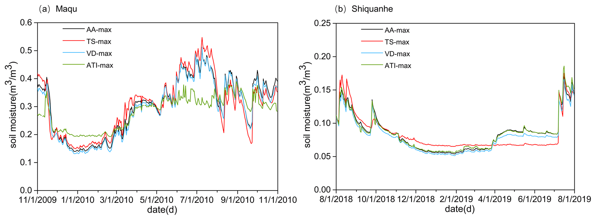
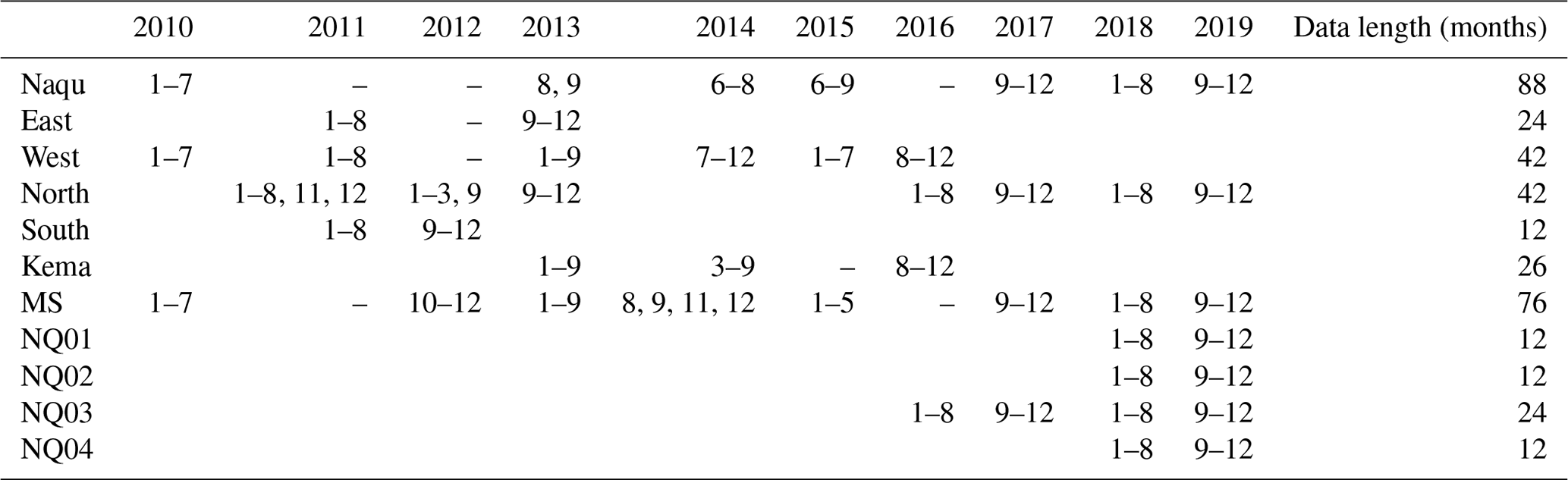
Figure 6 Comparisons of daily average SM for the (a) Maqu and (b) Shiquanhe networks produced by four upscaling methods with input of the maximum number of available SM monitoring sites. The date format is month/day/year.

Figure 6 shows the time series of daily average SM for the Maqu and Shiquanhe networks produced by the four upscaling methods based on the maximum number of available SM monitoring sites (hereafter “SM_AA-max”, “SM_VD-max”, “SM_TS-max”, and “SM_ATI-max”). Two different periods are selected for the two networks due to the fact that the number of available monitoring sites reaches the maximum in different periods for the two networks, e.g. 17 sites for Maqu between November 2009 and October 2010 and 12 sites for Shiquanhe between August 2018 and July 2019 (see Tables A2 and A4 in Appendix A). For the Maqu network, the SM_AA-max, SM_VD-max, and SM_TS-max are comparable to each other, while the SM_ATI-max deviates substantially during the winter (between December and February) and summer periods (between June and August). On the other hand, the SM_ATI-max for the Shiquanhe network is comparable to SM_AA-max and SM_VD-max, while SM_TS-max's behaviour is clearly different from the others. It seems that the ATI method performs better in the Shiquanhe network due to the existence of a stronger relationship between τ and θ in the desert ecosystem.

Table B1 lists the values of MRD (see Eq. B4 in Appendix B), σ(RD) (Eq. B3), and CEC (Eq. B6) calculated for the upscaled SM produced by the four upscaling methods. The CEC is used here to determine the most suitable upscaled SM that can best represent the areal conditions for the two networks. It can be found that the SM_AA-max consistently yields the lowest CEC values for both networks, indicating that the SM_AA-max can be used to represent actual areal conditions, which will thus be regarded as the ground truth for the following analysis (i.e. SM_truth). The arithmetic average of the dense in situ measurements was also used as the ground truth in other studies (Qin et al., 2013; Su et al., 2013) and was found to yield reliable results by van der Velde et al. (2021).

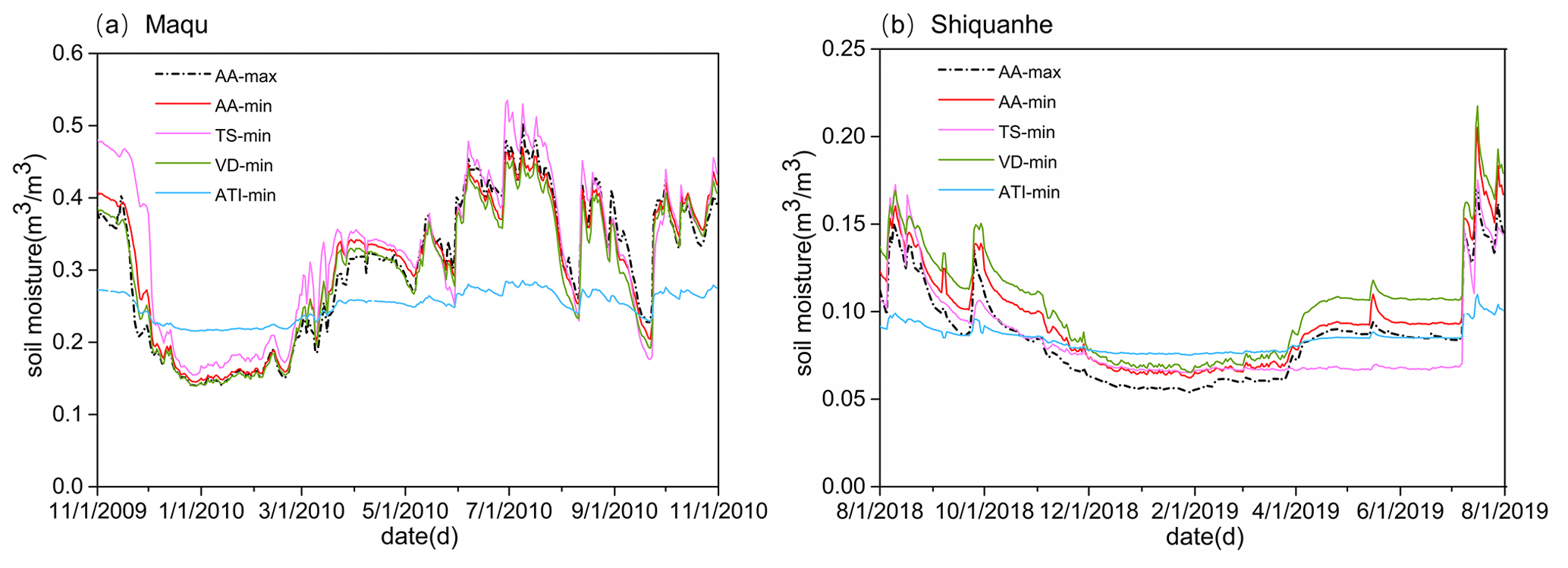
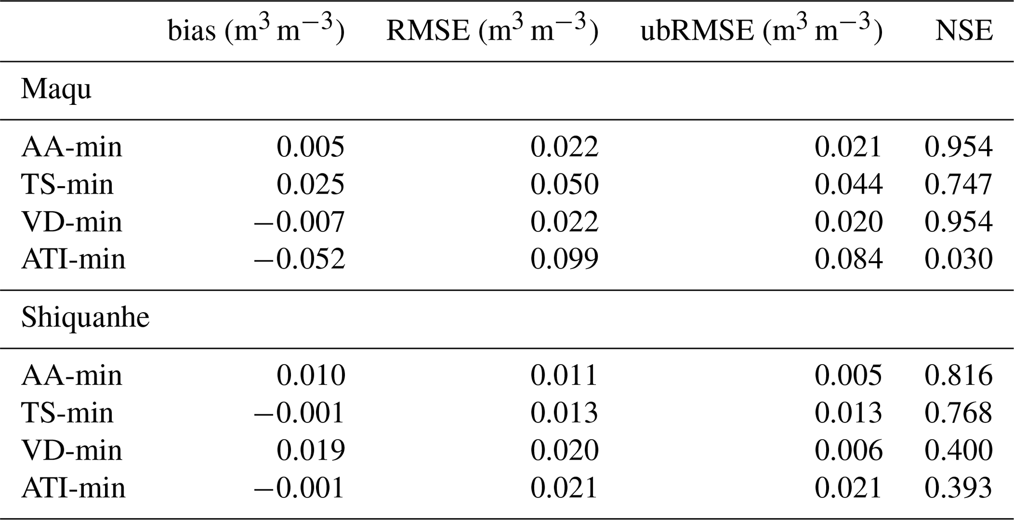
Figure 7 Comparisons of daily average SM for the (a) Maqu and (b) Shiquanhe networks produced by four upscaling methods with input of the minimum number of available SM monitoring sites. The date format is month/day/year.

As shown in Tables A2 and A4 (see Appendix A), the number of available SM monitoring sites decreased as time progressed. There are only three (i.e. CST05, NST01, and NST03) and four (i.e. SQ02, SQ03, SQ06, and SQ14) monitoring sites that provided more than 9 years of in situ SM measurement data for the Maqu and Shiquanhe networks, respectively (see Tables 2 and 3). This indicates that the minimum number of available monitoring sites can be used to produce the long-term (∼10-year) consistent upscaled SM is three and four for the Maqu and Shiquanhe networks, respectively. Figure 7 shows the daily average SM time series produced by the four upscaling methods based on the minimum available monitoring sites (hereafter “AA-min”, “TS-min”, “VD-min”, and “ATI-min”). The SM_truth obtained by the AA-max is also shown for comparison purposes. For the Maqu network, the upscaled SM produced by the AA-min, VD-min, and TS-min generally capture well the SM_truth variations, while the upscaled SM of the ATI-min shows dramatic deviations. Similarly, the upscaled SM produced by the AA-min and VD-min are consistent with the SM_truth for the Shiquanhe network with slight overestimations, while significant deviations are noted for the upscaled SM of the TS-min and ATI-min. Table B2 lists the error statistics (e.g. bias, RMSE, ubRMSE, and NSE) computed between the upscaled SM produced by these four upscaling methods with the input of the minimum available sites and the SM_truth. The upscaled SM produced by the AA-min shows better performance for both networks as indicated by the lower RMSE and higher NSE values in comparison to the other three upscaling methods.

Apart from the maximum and minimum number of available SM monitoring sites mentioned above, there are about 14, 10, 8, and 6 available monitoring sites during different time spans for the Maqu network, and for the Shiquanhe network there are about 11, 10, 6, and 5 available monitoring sites (see Tables A2 and A4 in Appendix A). Figure B2 shows the radar diagram of error statistics (i.e. RMSE and NSE) computed between the SM_truth and the upscaled SM produced by the four upscaling methods for different numbers of available monitoring sites. For the Maqu network, the performances of the AA and VD methods are better than the TS and ATI methods as indicated by smaller RMSEs and higher NSEs for all the estimations. A similar conclusion can be drawn for the Shiquanhe network, while the performance of the ATI method is largely improved when the number of available monitoring sites is not less than 10. It is interesting to note that the upscaled SM produced by the AA-min is comparable to those obtained with more sites (e.g. 10 sites) as indicated by comparable RMSE and NSE values for both networks. It indicates that the AA-min is suitable to produce long-term (∼10-year) upscaled SM for both networks, which yield RMSEs of 0.022 and 0.011 m³ m⁻³ for the Maqu and Shiquanhe networks in comparison to the SM_truth produced by the AA-max based on the maximum available monitoring sites.

4.2 Long-term analysis of upscaled soil moisture measurements

In this section, the AA-min is first adopted to produce the consecutive upscaled SM time series (hereafter “SM_AA-min”) for approximately a 10-year period for the Maqu and Shiquanhe networks. In addition, the other time series of upscaled SM are produced by the AA method with input of all available SM monitoring sites regardless of the continuity (hereafter “SM_AA-valid”), which is widely used to validate the various SM products (Dente et al., 2012b; Chen et al., 2013; Zheng et al., 2018b) for short periods (e.g. ≤2 years). This method may, however, lead to inconsistent SM time series for a long-term period due to the fact that the number of available sites is different in distinct periods (see Tables A2 and A4 in Appendix A). Trend analyses (see Sect. 3.2) are applied to both SM_AA-min and SM_AA-valid to investigate the impact of changes of available SM monitoring sites on the long-term (i.e. 10-year) trend.

Figure 8 Time series of SM_AA-min, SM_AA-valid, and precipitation for the (a) Maqu and (b) Shiquanhe networks for a 10-year period; the subplot highlights a 2-year period. The date format is month/day/year.

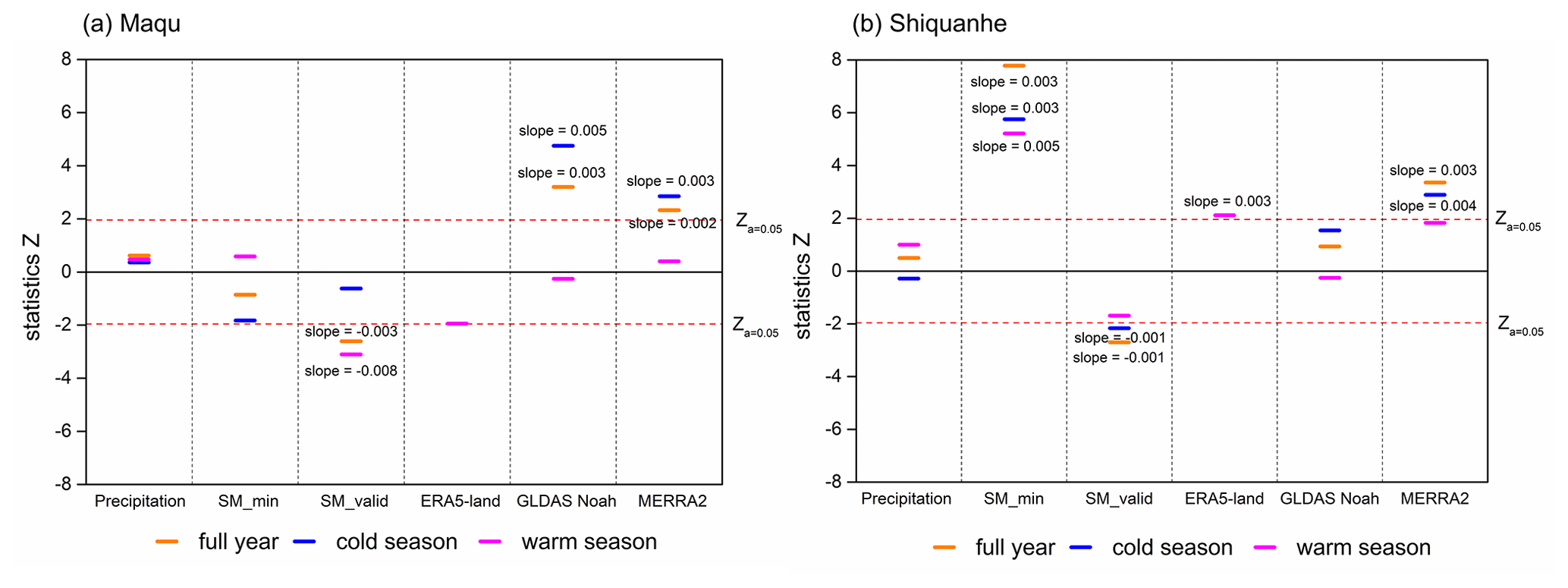
Figure 9 Mann–Kendall trend test and Sen's slope estimate for precipitation, SM_AA-min, SM_AA-valid, and model-based SM derived from the ERA5-Land, GLDAS Noah, and MERRA2 for a 10-year period for the (a) Maqu and (b) Shiquanhe networks.

Figure 8a shows the time series of SM_AA-min and SM_AA-valid along with the daily precipitation data for the Maqu network during the period between May 2009 and May 2019. The two time series of the SM show similar seasonality, with low values in winter due to frozen soils and high values in summer due to rainfall (see subplot of Fig. 8a). Deviations can be found between the SM_AA-min and SM_AA-valid especially for the period between 2014 and 2019, whereby the SM_AA-valid tends to produce smaller SM values in the warm season. Figure 9a shows further the Mann–Kendall trend test and Sen's slope estimate for the SM_AA-min, SM_AA-valid, and precipitation of the Maqu network area for the full year, warm seasons, and cold seasons in a 10-year period. As described in Sect. 3.2, the time series would present a monotonous trend if the absolute value of the Z metric were greater than a critical value, i.e. Z_0.05=1.96 in this study. The results show that no significant trend is found for both precipitation and SM_AA-min time series, while the SM_AA-valid shows a drying trend with a Sen's slope of −0.008 for warm seasons. The drying trend of the SM_AA-valid is caused by the change of available SM monitoring sites (see Table A2). Specifically, several monitoring sites (e.g. NST11–NST15) located in the wetter area were damaged from 2013 onwards, and four new monitoring sites (i.e. NST21–NST25) were installed in the drier area in 2015 (see Table 2), which affects the trend of the SM_AA-valid.

Figure 8b shows the time series of the SM_AA-min and SM_AA-valid along with the daily precipitation data for the Shiquanhe network during the period between August 2010 and August 2019. The two time series of the SM display a similar seasonality to that found for the Maqu network (see subplot of Fig. 8b). However, obvious deviations can be noticed for the inter-annual variations, and the SM_AA-valid tends to produce larger values before 2014 but smaller values thereafter. The Mann–Kendall trend test and Sen's slope estimate for the SM_AA-min, SM_AA-valid, and precipitation time series of the Shiquanhe network area are shown in Fig. 9b. The SM_AA-min demonstrates a wetting trend with a Sen's slope of 0.003, while an opposite drying trend is found for the SM_AA-valid due to a change in the number of available SM monitoring sites (see Table A4) similar to the results from the Maqu network. Specifically, several monitoring sites (e.g. SQ11 and SQ12) located in the wetter area were damaged around 2014, and five new monitoring sites (i.e. SQ17–21) were installed in the drier area in 2016 (see Table 3).

In summary, the SM_AA-valid is likely affected by the change of available SM monitoring sites over time that leads to an inconsistent trend with the SM_AA-min. This indicates that the SM_AA-min is superior to the SM_AA-valid for the production of the long-term consistent upscaled SM time series.

4.3 Application of the long-term upscaled soil moisture to validate the model-based products

In this section, the long-term upscaled SM time series (i.e. SM_AA-min) produced for the two networks are applied to validate the reliability of three model-based SM products – i.e. ERA5-Land, MERRA2, and GLDAS Noah – to demonstrate the uniqueness of this dataset for validating existing reanalysis datasets for a long-term period (∼10 years). Since the ERA5-Land product provides only total volumetric soil water content, the period when the soil is subject to freezing and thawing (i.e. November–April) is excluded for this evaluation.

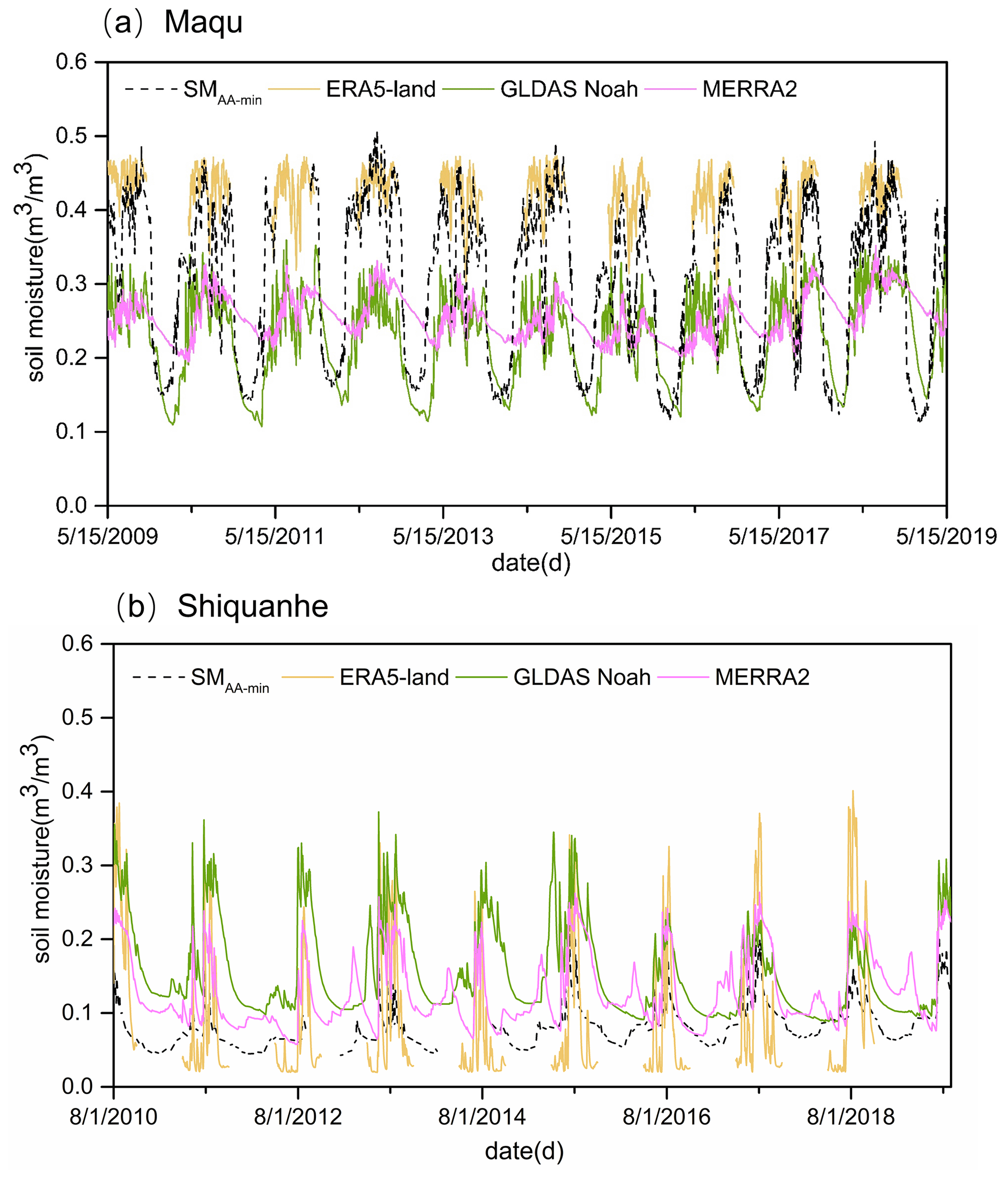
Figure 10 A 10-year time series of model-based SM derived from the ERA5-Land, MERRA2, and GLDAS Noah products and the upscaled SM (SM_AA-min) for the (a) Maqu and (b) Shiquanhe networks. The date format is month/day/year.

Figure 10a shows the time series of SM_AA-min and daily average SM data derived from the three products for the Maqu network during the period between May 2009 and May 2019. The error statistics, i.e. bias and RMSE, computed between the three products and the SM_AA-min for both warm (May–October) and cold seasons (November–April) are given in Table 5. Although the three products generally capture the seasonal variations of the SM_AA-min, the magnitude of the temporal SM variability is underestimated. Both GLDAS Noah and MERRA2 products underestimate the SM measurements during the warm season, leading to biases of about −0.112 and −0.113 m³ m⁻³, respectively. This may be due to the fact that the land surface models (LSMs) adopted for producing these products do not consider the impact of vertical soil heterogeneity caused by organic matter content, which is widely present in the soil Tibetan surface (Chen et al., 2013; Zheng et al., 2015a). In addition, the MERRA2 product overestimates the SM measurements during the cold season with a bias of about 0.006 m³ m⁻³. The ERA5-Land product is able to capture the magnitude of SM_AA-min dynamics in the warm season but has a larger volatility and yields a RMSE of about 0.067 m³ m⁻³. The trend analysis for the three model-based SM products is shown in Fig. 9a as well. All three products do not show a significant trend in warm seasons like the SM_AA-min, while the GLDAS Noah and MERRA2 products show a wetting trend in cold seasons that is in disagreement with the SM_AA-min trend.

Table 5 Error statistics computed between the SM_AA-min and the three model-based SM products for the Maqu and Shiquanhe networks.

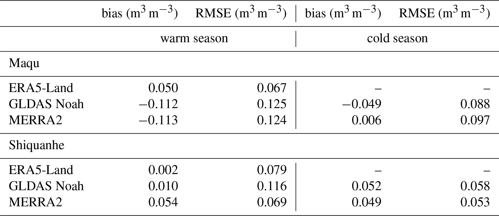
Figure 10b shows the time series of SM_AA-min and daily SM data derived from the three products for the Shiquanhe network area during the period between August 2010 and August 2019, and the corresponding error statistics are given in Table 5 as well. Although the three products generally capture the seasonal variations of the SM_AA-min, both GLDAS Noah and MERRA2 products overestimate the SM_AA-min during the entire study period, leading to positive biases, and a positive bias (about 0.002 m³ m⁻³) is also found in the ERA5-Land product for the warm season. The trend analyses for the three SM products are also shown in Fig. 9b. Both the ERA5-Land and MERRA2 products are able to reproduce the wetting trend found for the SM_AA-min, while the GLDAS Noah product is not able to capture the trend.

In summary, the currently model-based SM products do not provide a reliable representation of the trend and the dynamics of measured SM in the long term (∼10 years) in the grassland and desert ecosystems that dominate the Tibetan landscape.

5 Discussion

As shown in previous sections, the number of available SM monitoring sites in the Tibet-Obs generally changes with time. For instance, several monitoring sites of the Maqu network located in the wetter area have been damaged since 2013, and four new monitoring sites were installed in the drier area in 2015, which affects the trend of SM time series (i.e. SM_AA-valid shown in Sect. 4.2). On the other hand, the 10-year upscaled SM data (i.e. SM_AA-min) produced in this study utilizing three and four monitoring sites with long-term continuous measurements would yield RMSEs of about 0.022 and 0.011 m³ m⁻³ for the Maqu and Shiquanhe networks, respectively (see Sect. 4.1). Therefore, to provide a higher-quality continuous SM time series for the future, it is necessary to find an appropriate strategy to maintain the monitoring sites of Tibet-Obs. This section discusses the possible strategies with the Maqu and Shiquanhe networks as examples.

At first, a sensitivity analysis is conducted to quantify the impact of the number of monitoring sites on the regional SM estimate. The SM time series described in Sect. 4.1 (i.e. November 2009–October 2010 for the Maqu network and August 2018–July 2019 for the Shiquanhe network) is used to test the sensitivity, and there are in total 17 and 12 available monitoring sites for the Maqu and Shiquanhe networks, respectively. Taking the Maqu network as an example, we randomly pick different numbers of sites from 1 to 16 of the 17 sites to make up different combinations and then compute the RMSEs of the averaged SM obtained with these combinations (Famiglietti et al., 2008; Zhao et al., 2013). These RMSEs are further grouped into nine levels ranging from 0.004 to 0.02 m³ m⁻³, and the percentage of the combinations falling into each level is summarized in Table 6. In general, the percentage increases with an increasing number of monitoring sites at any RMSE level. It can be noted that more than 50 % of combinations are able to comply with the RMSE requirement of 0.004 m³ m⁻³ if the number of available monitoring sites is 16 and 11 in the Maqu and Shiquanhe networks, respectively. If the number of available monitoring sites is more than 13 and 6 in the Maqu and Shiquanhe networks, respectively, then about 60 % of combinations with 13 sites (6 sites) are able to comply with the RMSE requirement of 0.01 m³ m⁻³. For a RMSE of 0.02 m³ m⁻³, more than 50 % of combinations comply with this requirement if the number of available monitoring sites is more than 7 and 3 for the two networks, respectively. In summary, the number of monitoring sites required to maintain current networks depends on the defined RMSE requirement.

Table 6 Percentages of the site combinations that fall into an accuracy requirement in terms of RMSE.

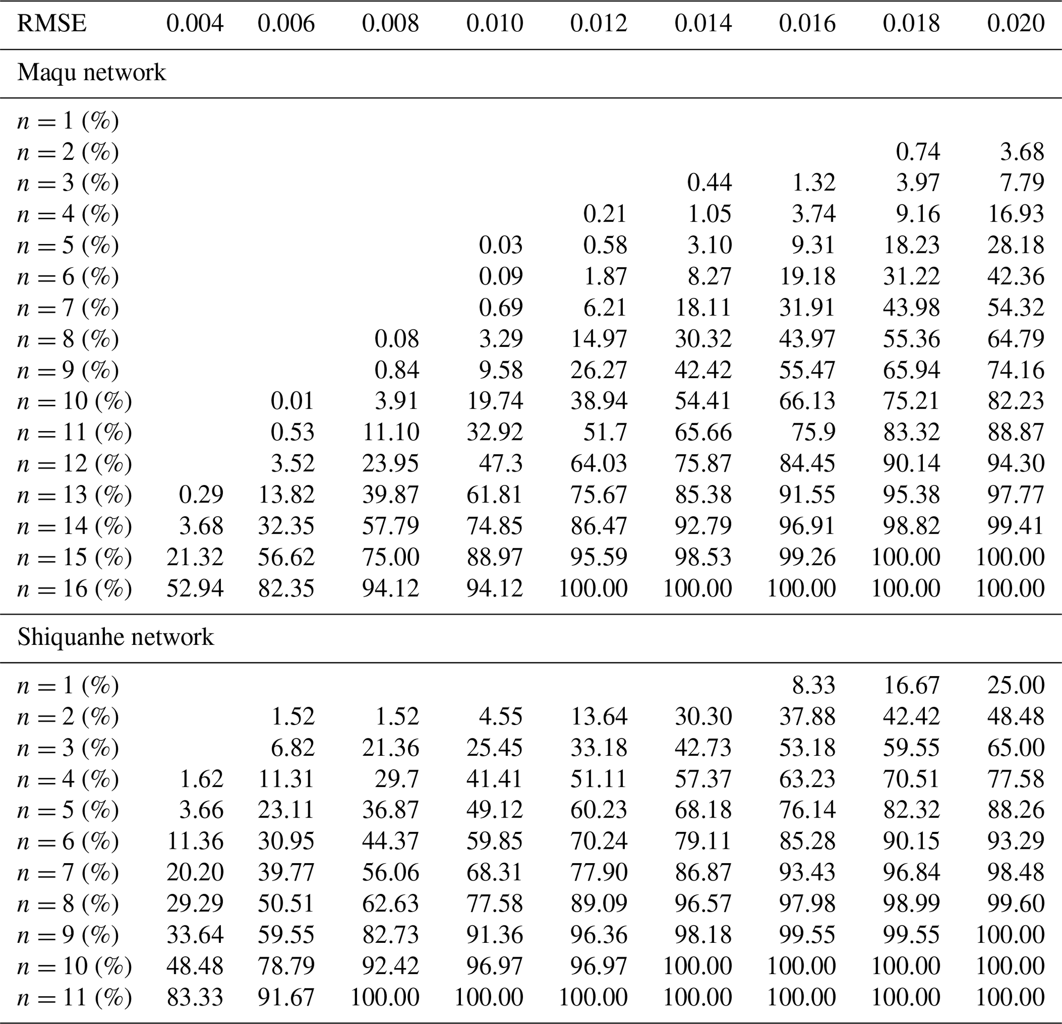
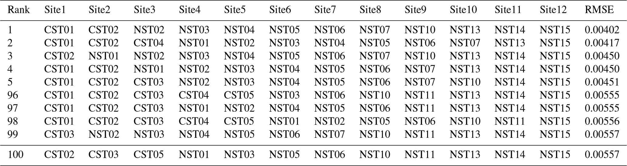
As shown in Sect. 4.1, the usage of a minimum number of sites (i.e. three for Maqu and four for Shiquanhe) with about 10-year continuous measurements yields RMSEs of 0.022 and 0.011 m³ m⁻³ for the Maqu and Shiquanhe networks, respectively. Since there are still 12 monitoring sites providing SM measurements for both networks until 2019 (see Tables 2 and 3), it is possible to decrease the RMSEs when the selected permanent monitoring sites are appropriately determined. For the Shiquanhe network, the optimal strategy is to keep the current 12 monitoring sites, which is exactly the combination used in Sect. 4.1. For the Maqu network, it can be found that about 3.52 % of combinations with 12 sites could yield the minimum RMSE of 0.006 m³ m⁻³ (see Table 6). In order to find the optimal combination with 12 sites for the Maqu network, all the possible combinations (i.e. 6188 combinations) are ranked by RMSE values from the smallest to largest, and Table 7 lists the examples of ranking 1st–5th and 95th–100th. It can be noted that the 100th combination contains the largest number of currently available monitoring sites (i.e. seven sites, including CST03, CST05, NST01, NST03, NST05, NST06, and NST10) with a RMSE of less than 0.006 m³ m⁻³. Therefore, the 100th combination of 12 monitoring sites (as shown in Table 7) is suggested for the Maqu network.

Table 7 The combinations of monitoring sites ranked by RMSE values of average SM in the Maqu network.

In summary, it is suggested to maintain the current 12 monitoring sites for the Shiquanhe network, while for the Maqu network it is suggested to restore five old monitoring sites, i.e. CST02, NST11, NST13, NST14, and NST15.

6 Data availability

The 10-year (2009–2019) surface SM dataset is freely available from the 4TU.ResearchData repository at https://doi.org/10.4121/12763700.v7 (Zhang et al., 2020). The original in situ SM data, the upscaled SM data, and the supplementary data are stored in .xlsx files. A user guide document is given to introduce the content of the dataset, the status of the Tibet-Obs, and the online dataset utilized in the study.

7 Conclusions

In this paper, we report on the status of the Tibet-Obs and present the long-term in situ SM and spatially upscaled SM dataset for the period 2009–2019. In general, the number of available SM monitoring sites decreased over time due to damage to sensors. Until 2019, there are only three and four sites that provide an approximately 10-year consistent SM time series for the Maqu and Shiquanhe networks, respectively. Comparisons between four upscaling methods – i.e. arithmetic averaging (AA), Voronoi diagram (VD), time stability (TS), and apparent thermal inertia (ATI) – show that the AA method with input of the maximum number of available SM monitoring sites (AA-max) can be used to represent the actual areal SM conditions (SM_truth). The arithmetic average of the three and four monitoring sites with long-term continuous measurements (AA-min) is found to be most suitable to produce the upscaled SM dataset for the period 2009–2019, which yields RMSEs of 0.022 and 0.011 m³ m⁻³ for the Maqu and Shiquanhe networks in comparison to the SM_truth.

Trend analysis of the approximately 10-year upscaled SM time series produced by the AA-min (SM_AA-min) shows that the Shiquanhe network in the western part of the TP gets wet, while no significant trend is found for the Maqu network in the east. The usage of all the available monitoring sites each year leads to inconsistent time series of SM that cannot capture the trend of SM_AA-min reliably. Comparisons between the SM_AA-min and the model-based SM products from the ERA5-Land, GLDAS Noah, and MERRA2 further demonstrate that current model-based SM products still show deficiencies in representing the trend and the dynamics of the SM measured on the TP. Moreover, strategies for maintaining the Tibet-Obs are provided, and it is suggested to maintain the 12 current operational sites for the Shiquanhe network, while for the Maqu network it is suggested to restore five old sites.

The 10-year (2009–2019) surface SM dataset presented in this paper includes the 15 min in situ measurements taken at a depth of 5 cm collected from three regional-scale networks (i.e. Maqu, Naqu, and Ngari including Ali and Shiquanhe) of the Tibet-Obs and the spatially upscaled SM datasets produced by the AA-min for the Maqu and Shiquanhe networks. This dataset is valuable for calibrating/validating long-term satellite- and model-based SM products, evaluation of SM upscaling methods, development of data fusion methods, and quantifying the coupling of SM with precipitation at a 10-year scale.

Appendix A: Basic information of the Tibet-Obs

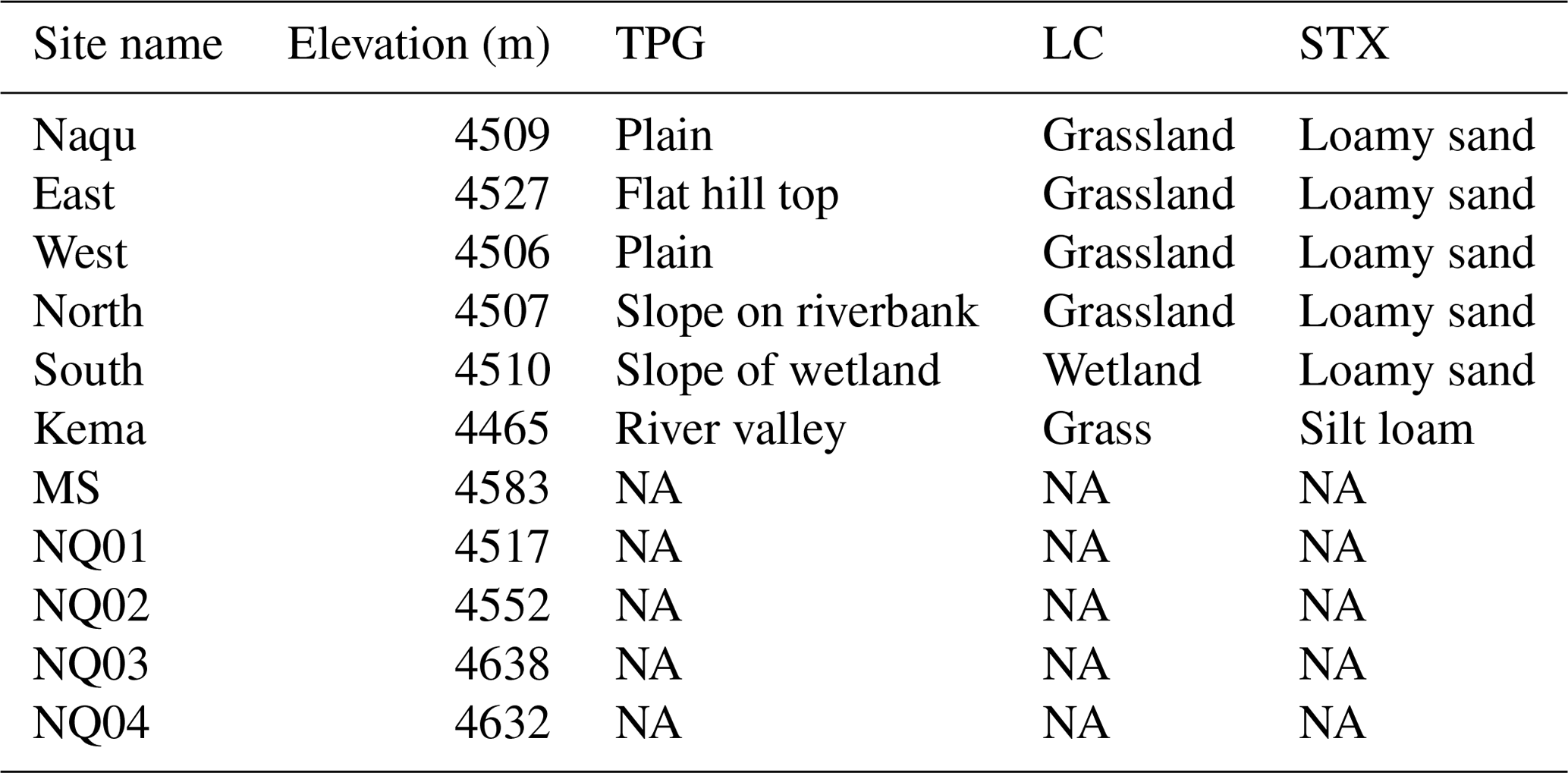
Table A1 Site information of the Maqu network (site name, elevation, topography (TPG), land cover (LC), soil texture at 5–15 cm depth (STX), soil bulk density at 5 cm depth (BD), soil organic matter content at 5–15 cm depth (OMC), not available (NA); BD and OMC values are measured in the laboratory).

Table A2 Soil moisture with temporal persistence for the Maqu network. Cells with a hyphen represent that no data are missing; cells with “M” indicate data are missing with little influence.

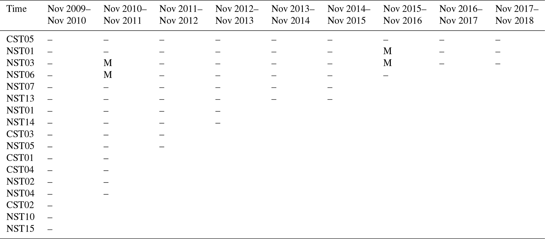
Table A3 Same as Table A1 but for the Ngari network (BD and OMC data are not available).

Table A4 Same as Table A2 but for the Shiquanhe network.

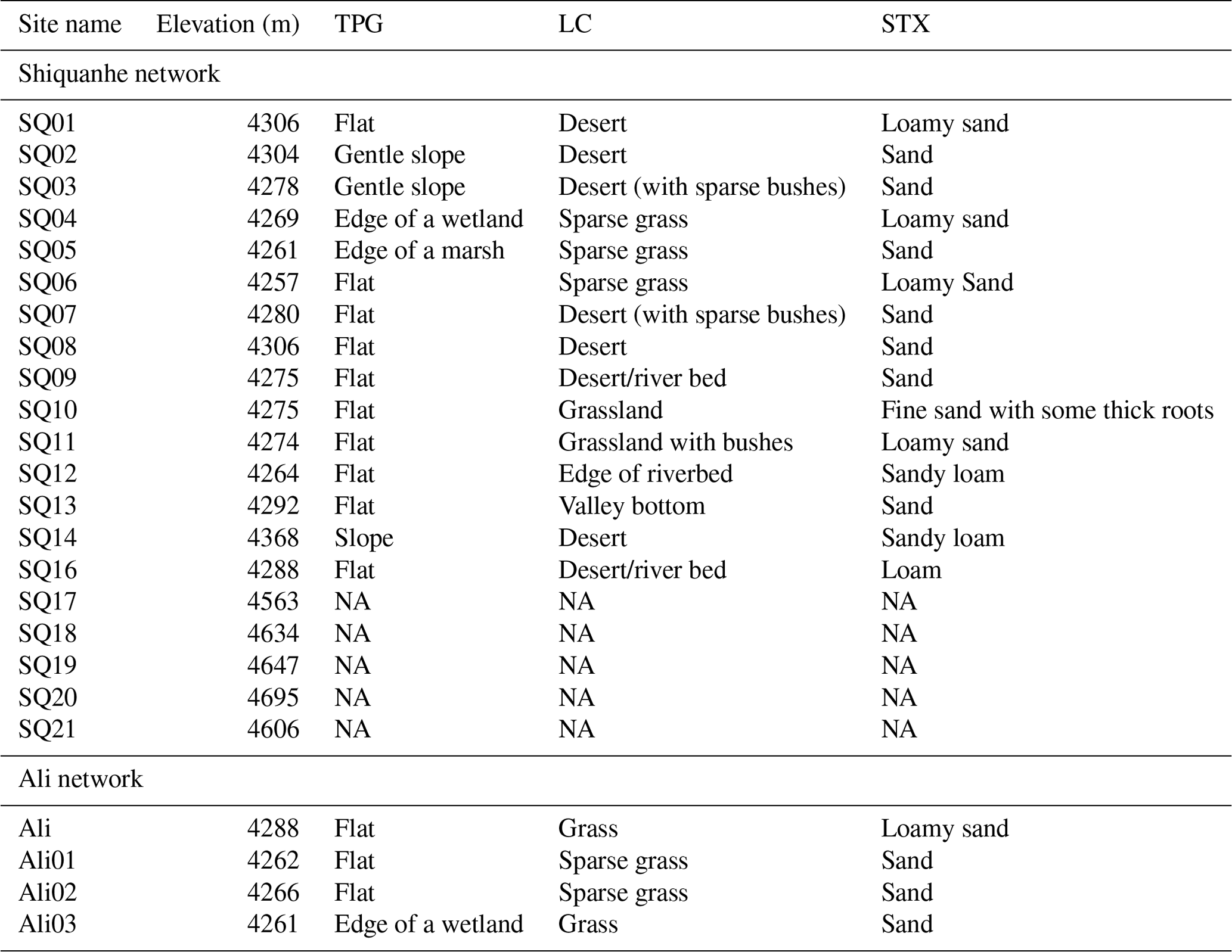
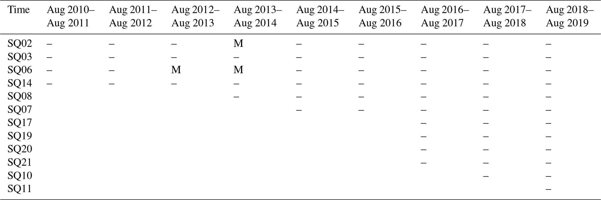
Table A5 Same as Table A1 but for the Naqu network (BD and OMC data are not available).

Appendix B: Spatial upscaling methods

B1 Arithmetic averaging

The arithmetic averaging method assigns an equal weight coefficient to each SM monitoring site of the network, which can be formulated as

$$\begin{array}{}\text{(B1)}& {\stackrel{\mathrm{‾}}{\mathit{\theta }}}_t^{\text{ups}}={\displaystyle \frac{\mathrm{1}}{N}}\sum _{i=\mathrm{1}}^N{\mathit{\theta }}_{t,i}^{\text{obs}},\end{array}$$

where i represents the ith SM monitoring site.

B2 Voronoi diagram

The Voronoi diagram method divides the network area into several parts according to the distances between each SM monitoring site. This approach determines the weight of each site (w_i (–)) based on the geographic distribution of all the SM monitoring sites within the network area, which can be formulated as

$$\begin{array}{}\text{(B2)}& {\stackrel{\mathrm{‾}}{\mathit{\theta }}}_t^{\text{ups}}={\displaystyle \frac{{\sum }_{i=\mathrm{1}}^N{w}_i{\mathit{\theta }}_{t,i}^{\text{obs}}}{{\sum }_{i=\mathrm{1}}^N{w}_i}}.\end{array}$$

B3 Time stability

The time stability method is based on the assumption that the spatial SM pattern over time tends to be consistent (Vachaud et al., 1985), and the most stable site can be regarded as the representative site of the network. For each SM monitoring site i within the time window (M days in total), the mean relative difference MRD_i (–) and standard deviation of the relative difference σ(RD_i) (–) are estimated as

$$\begin{array}{}\text{(B3)}& {\displaystyle }& {\displaystyle }\mathit{\sigma }\left({\text{RD}}_i\right)=\sqrt{{\displaystyle \frac{\mathrm{1}}{M-\mathrm{1}}}\sum _{t=\mathrm{1}}^M{\left({\text{RD}}_{t,i}-{\text{MRD}}_i\right)}^{\mathrm{2}}},\text{(B4)}& {\displaystyle }& {\displaystyle }{\text{MRD}}_i={\displaystyle \frac{\mathrm{1}}{M}}\sum _{t=\mathrm{1}}^M{\displaystyle \frac{{\mathit{\theta }}_{t,i}^{\text{obs}}-\stackrel{\mathrm{‾}}{{\mathit{\theta }}_t^{\text{obs}}}}{\stackrel{\mathrm{‾}}{{\mathit{\theta }}_t^{\text{obs}}}}},\text{(B5)}& {\displaystyle }& {\displaystyle }{\text{RD}}_{t,i}={\displaystyle \frac{{\mathit{\theta }}_{t,i}^{\text{obs}}-\stackrel{\mathrm{‾}}{{\mathit{\theta }}_t^{\text{obs}}}}{\stackrel{\mathrm{‾}}{{\mathit{\theta }}_t^{\text{obs}}}}},\end{array}$$

where ${\mathit{\theta }}_{t,i}^{\text{obs}}$ (m³ m⁻³) represents the SM measured on the tth day at the ith monitoring site, $\stackrel{\mathrm{‾}}{{\mathit{\theta }}_t^{\text{obs}}}$ (m³ m⁻³) represents the mean SM measured at all available monitoring sites on the tth day. MRD_i quantifies the bias of each SM monitoring site to identify a particular location as wetter or drier than the regional mean, and σ(RD_i) characterizes the precision of the SM measurement. Jacobs et al. (2004) combined the above two statistical metrics as a comprehensive evaluation criterion (CEC_i (–)):

$$\begin{array}{}\text{(B6)}& {\text{CEC}}_i=\sqrt{{\left({\text{MRD}}_i\right)}^{\mathrm{2}}+\mathit{\sigma }{\left({\text{RD}}_i\right)}^{\mathrm{2}}}.\end{array}$$

The most stable site is identified by the lowest CEC_i value.

B4 Apparent thermal inertia

The apparent thermal inertia (ATI) method is based on the close relationship between apparent thermal inertia (τ (K⁻¹)) and SM (θ (m³ m⁻³)) (Van doninck et al., 2011; Veroustraete et al., 2012). If the true areal SM (${\stackrel{\mathrm{‾}}{\mathit{\theta }}}_t^{\text{tru}}$ (m³ m⁻³)) is available, then the weight vector β can be derived by the ordinary least-squares (OLS) method, which minimizes the cost function J as

$$\begin{array}{}\text{(B7)}& J=\sum _{t=\mathrm{1}}^M{\left({\mathit{\theta }}_t^{\text{tru}}-{\mathit{\beta }}^T{\mathit{\theta }}_t^{\text{obs}}\right)}^{\mathrm{2}}.\end{array}$$

However, the ${\mathit{\theta }}_t^{\text{tru}}$ (m³ m⁻³) is usually not available in practice, and the representative SM (${\stackrel{\mathrm{‾}}{\mathit{\theta }}}_t^{\text{rep}}$ (m³ m⁻³)) is thus introduced, which contains random noise but with no bias. Since the OLS method may result in overfitting with usage of the ${\stackrel{\mathrm{‾}}{\mathit{\theta }}}_t^{\text{rep}}$, a regularization term is introduced, and Eq. (B7) can be re-formulated as (Tarantola, 2005)

$$\begin{array}{ll}{\displaystyle }J=& {\displaystyle }\sum _{t=\mathrm{1}}^M\left({\stackrel{\mathrm{‾}}{\mathit{\theta }}}_t^{\text{rep}}-{\mathit{\beta }}^T{\mathit{\theta }}_t^{\text{obs}}\right){\mathit{\sigma }}^{-\mathrm{2}}\\ \text{(B8)}& {\displaystyle }& {\displaystyle }\cdot \left({\stackrel{\mathrm{‾}}{\mathit{\theta }}}_t^{\text{rep}}-{\mathit{\beta }}^T{\mathit{\theta }}_t^{\text{obs}}\right)+R{\mathit{\beta }}^T\mathit{\beta },\end{array}$$

where σ (m³ m⁻³) represents the standard deviation of ${\stackrel{\mathrm{‾}}{\mathit{\theta }}}_t^{\text{rep}}$, and R (–) is the regularization parameter.

The core issue of the ATI approach is to obtain the ${\stackrel{\mathrm{‾}}{\mathit{\theta }}}_t^{\text{rep}}$ and minimize the cost function of Eq. (B8) to obtain β and R. The ${\stackrel{\mathrm{‾}}{\mathit{\theta }}}_t^{\text{rep}}$can be retrieved from the apparent thermal inertia τ via empirical regression g(τ), and τ has a strong connection with the surface status, e.g. land surface temperature and albedo, which is defined as

$$\begin{array}{}\text{(B9)}& \mathit{\tau }=C{\displaystyle \frac{\mathrm{1}-a}{A}},\end{array}$$

where C (–) represents the solar correction factor, a (–) represents the surface albedo, and A (K) represents the amplitude of the diurnal temperature cycle. The albedo and land surface temperature data obtained from the MODIS MCD43A3 and MYD11A1/MOD11A1 version 6 products are used to derive the ATI according to Eq. (B9) in this study.

The solar correlation factor C in Eq. (B9) is computed as

$$\begin{array}{ll}{\displaystyle }C=& {\displaystyle }\sin \mathit{\phi }\sin \mathit{\delta }{\left(\mathrm{1}-{\tan }^{\mathrm{2}}\mathit{\phi }{\tan }^{\mathrm{2}}\mathit{\delta }\right)}^{\mathrm{1}/\mathrm{2}}\\ \text{(B10)}& {\displaystyle }& {\displaystyle }+\cos \mathit{\phi }\cos \mathit{\delta }\arccos (-\tan \mathit{\phi }\tan \mathit{\delta }),\end{array}$$

with

$$\begin{array}{ll}{\displaystyle }\mathit{\delta }=& {\displaystyle }\mathrm{0.00691}-\mathrm{0.399912}\cos \left(\mathit{\gamma }\right)+\mathrm{0.070257}\sin \left(\mathit{\gamma }\right)\\ {\displaystyle }& {\displaystyle }-\mathrm{0.006758}\cos \left(\mathrm{2}\mathit{\gamma }\right)+\mathrm{0.000907}\sin \left(\mathrm{2}\mathit{\gamma }\right)\\ \text{(B11)}& {\displaystyle }& {\displaystyle }-\mathrm{0.002697}\cos \left(\mathrm{3}\mathit{\gamma }\right)+\mathrm{0.00148}\sin \left(\mathrm{3}\mathit{\gamma }\right)\end{array}$$

and

$$\begin{array}{}\text{(B12)}& \mathit{\gamma }={\displaystyle \frac{\mathrm{2}\mathit{\pi }(n_{\mathrm{d}}-\mathrm{1})}{\mathrm{365.25}}},\end{array}$$

where φ represents the latitude (rad), δ represents the solar declination (rad), and n_d represents the Julian day number.

The amplitude of the diurnal land surface temperature (LST) A is estimated as LST_max−LST_min for a single day. Finally, we use the regression analysis between in situ SM measurements (θ) at each monitoring site and corresponding ATI (τ) to obtain the g(⋅) form.

There are 17 and 12 monitoring sites participating in the regression analysis for the Maqu and Shiquanhe networks during the periods of November 2009–October 2010 and August 2018–July 2019, respectively. The ATI cannot be obtained for each monitoring site on every day since the satellite-based LST data are contaminated by clouds. In order to make full use of the data, we make the ATI–SM pair for the first monitoring site on the first day no. 1, the pair for the 17th (12th) monitoring site in the Maqu (Shiquanhe) network on the first day no. 17 (no. 12), the pair for the first monitoring site on the second day no. 18 (no. 13), and so on. Later on, we select a certain number of ATI–SM pairs (e.g. 40, 50, 60, 70, 80, 90, and 100) as a group to compute the averaged ATI and SM and construct the most reliable (i.e. with the maximum R²) regression relationship between them. If the ATI or SM data on one day are missing, this pair is ignored. As shown in Fig. B1, the empirical relationship is generated from 80 pairs of ATI and SM averaged for the Maqu and Shiquanhe networks.

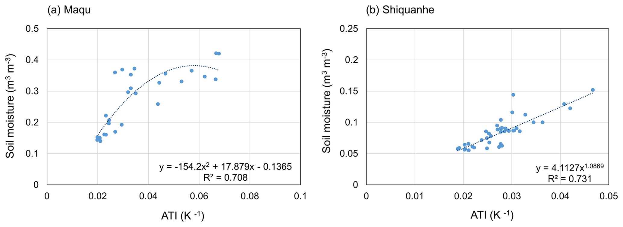
Figure B1 Empirical relationship between 80 pairs of ATI and SM averaged for the (a) Maqu and (b) Shiquanhe networks.

When the empirical relationship g(⋅) is determined, the regional-average SM can be derived from grid-averaged ATI by the function g(⋅), which is regarded as ${\stackrel{\mathrm{‾}}{\mathit{\theta }}}_t^{\text{rep}}$ in Eq. (B8). Finally, the optimal β ($\widehat{\mathit{\beta }}$) is obtained by minimizing the cost function (i.e. Eq. B8), and the upscaled SM can be estimated as

$$\begin{array}{}\text{(B13)}& {\stackrel{\mathrm{‾}}{\mathit{\theta }}}_t^{\text{ups}}=\widehat{\mathit{\beta }}{\mathit{\theta }}_t^{\text{obs}}.\end{array}$$

Detailed description of the ATI method can be found in Qin et al. (2013).

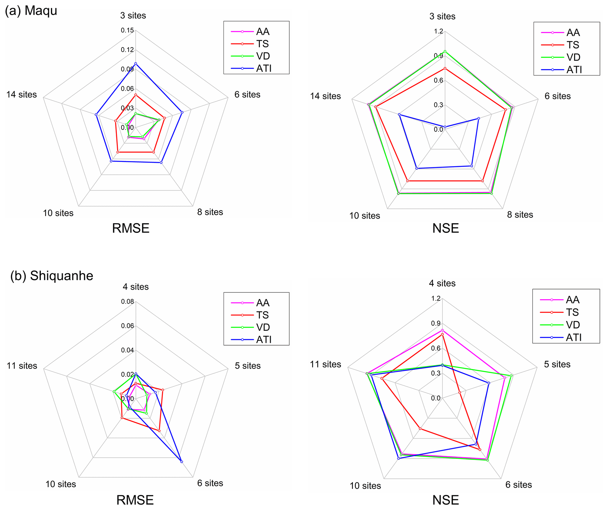
Figure B2 Radar diagram of error statistics (i.e. RMSE and NSE) computed between the SM_truth produced by the AA-max and the upscaled SM produced by the four upscaling methods with input of a different number of available monitoring sites for the (a) Maqu and (b) Shiquanhe networks.

Table B1 Evaluation metrics computed for the upscaled SM produced with four methods with input of the maximum available monitoring sites. The bold font represents the best performance with the lowest CEC value.

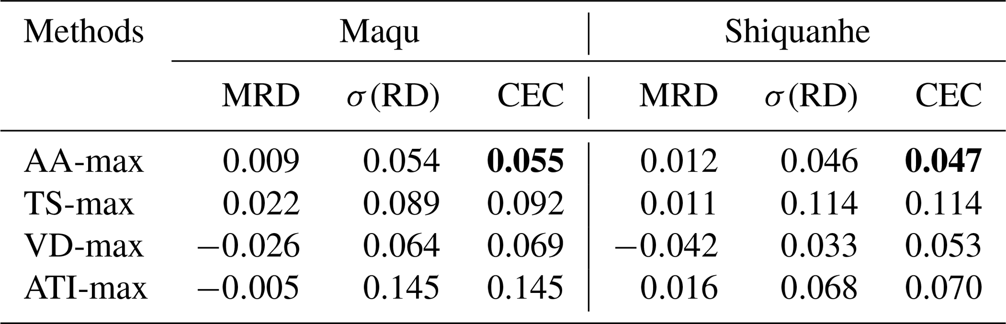
Table B2 Error statistics computed between the SM obtained by the four upscaling methods with input of the minimum available monitoring sites and the SM_truth produced by the AA-max for the Maqu and Shiquanhe networks.