the Creative Commons Attribution 4.0 License.
the Creative Commons Attribution 4.0 License.
 | 09 Jun 2021
An integrated marine data collection for the German Bight – Part 2: Tides, salinity, and waves (1996–2015)
Andreas Plüß
Romina Ihde
Janina Freund
Norman Dreier
Edgar Nehlsen
Nico Schrage
Peter Fröhle
Frank Kösters
Marine spatial planning requires reliable data for, e.g., the design of coastal structures, research, or sea level rise adaptation. This task is particularly ambiguous in the German Bight (North Sea, Europe) because a compromise must be found between economic interests and biodiversity since the environmental status is monitored closely by the European Union. For this reason, we have set up an open-access, integrated marine data collection for the period from 1996 to 2015. It provides bathymetry, surface sediments, tidal dynamics, salinity, and waves for the German Bight and is of interest to stakeholders in science, government, and the economy. This part of a two-part publication presents data from numerical hindcast simulations for sea surface elevation, depth-averaged current velocity, bottom shear stress, depth-averaged salinity, wave parameters, and wave spectra. As an improvement to existing data collections, our data represent the variability in the bathymetry by using annually updated model topographies. Moreover, we provide data at a high temporal and spatial resolution (Hagen et al., 2020b); i.e., numerical model results are gridded to 1000 m at 20 min intervals (https://doi.org/10.48437/02.2020.K2.7000.0004). Tidal characteristic values (Hagen et al., 2020a), such as tidal range or ebb current velocity, are computed based on numerical modeling results (https://doi.org/10.48437/02.2020.K2.7000.0003). Therefore, this integrated marine data collection supports the work of coastal stakeholders and scientists, which ranges from developing detailed coastal models to handling complex natural-habitat problems or designing coastal structures.
- Article
(16968 KB) - Full-text XML
-
Supplement
(752 KB) - BibTeX
- EndNote


The North Sea on the northwest European shelf is a region where competing interests of economic growth and the protection of future ecosystem services collide. On the one hand, there is, for example, a significant increase in energy produced by offshore wind farms as part of the European Union's blue growth initiative; on the other hand, strict legislation (e.g., by the Marine Strategy Framework Directive) has to be complied with to ensure a good environmental status. Pursuing both goals requires a reliable database of hydrographical parameters to assess both economic prospects and ecological change.
The hydrography of the North Sea is characterized by tides and surge from the North Atlantic, local wind and wave effects, and the interaction with adjacent estuaries (Otto et al., 1990). This variability is superimposed by long-term changes such as sea level rise (Idier et al., 2017), spatially varying change in tidal range (Jänicke et al., 2021; Müller, 2011), seasonality (Müller et al., 2014), and changing seabed morphology (Winter, 2011; Benninghoff and Winter, 2019). An unusually broad spectrum of field data and scientific knowledge is available at the study site because hydrographic parameters of the North Sea are monitored by one of the densest measurement networks worldwide. However, long-term measurements, such as sea surface elevation or salinity depend on gauge locations, whereas spatial measurements, such as ADCP campaigns, often lack temporal coverage. Remote sensing attempts to bridge this gap, but a temporal resolution in the order of individual tidal events is still missing.
In the Earth sciences and oceanography, numerical process-based models are applied to fill data gaps for a user-specified model domain. Hindcast model data products for the German Bight started with unstructured data from the coastDat data (Weisse and Plüß, 2006), which have been updated to coastDat2 (Geyer, 2014; Groll and Weisse, 2017). CoastDat2 contains sea surface elevation, current velocity, and wave climate products at a regular 1.6 km spatial resolution with hourly time intervals (waves 5.5 km regular grid, 3 h intervals). Similarly to coastDat2, the ERA-40 data set describes the wind and wave climate. ERA-40 demonstrates higher skill when compared to measurements, yet it covers a shorter time period (Reistad et al., 2011). There are similar data from coastal engineering projects, e.g., the AufMod data collection (Heyer et al., 2015), which provides annual tidal characteristic values as polyarea shape files (i.e., tidal range, tidal high water, etc.) and annual bathymetries on a 50 m raster from 1982 to 2012. Other data products cover the northwest European shelf region (e.g., https://marine.copernicus.eu/, last access: 7 June 2021) or the entire globe (e.g., global tides of the finite element solution, FES, by Lyard et al., 2006) and are therefore limited to a coarse grid resolution near the coast (minimum 2.5 km regular grids, usually much coarser, on the European shelf).
As pointed out by Groll and Weisse (2017) and Rasquin et al. (2020), a high spatial resolution of data sets is required in the German Bight to properly resolve the morphologically complex nearshore area in the German Bight, which is characterized by islands, extensive tidal flats, and deep channels with a typical width of 10 km to less than 1 km. None of the data products mentioned above reach that resolution. Furthermore, a typical tidal cycle in the North Sea takes about 12.4 h and contains two peaks in current velocity (flood and ebb). Hence, it can be argued that a 1 h resolution is too coarse to represent peaks in both sea surface elevation and current velocity. Additionally, almost none of the hindcasts above use annually varying bathymetry for numerical model simulations which is crucial in the morphodynamically highly active Wadden Sea (Winter, 2011; Benninghoff and Winter, 2019), as bathymetry variation in the nearshore area has been shown to have an impact on large-scale tidal dynamics (Jacob et al., 2016).
For further progress in terms of spatial and temporal resolution, a 20-year hindcast marine data collection for the time from 1996 to 2015 based on numerical modeling results with annually updated bathymetry is established. Data products include sea surface elevation, depth-averaged current velocity, bed shear stress, depth-averaged salinity, wave parameters, and wave spectra in the German Bight at a high spatial (1000 m by 1000 m) and temporal (20 min intervals) resolution. Numerical modeling at this temporal and spatial scale has become possible with the availability of high-resolution bathymetry (Sievers et al., 2021), surface sediments, reanalyzed meteorology (Bollmeyer et al., 2015), and input from global modeling products such as FES. An in-depth description of data-based products can be found in the accompanying paper of Sievers et al. (2021). In Sievers et al. (2021), we describe the calculation of annual bathymetry and decadal surface sediment data from observations and discuss limitations, data sources, and accuracy. Stakeholders from scientific, commercial, and governmental communities have been involved to ensure optimal usability of our data collection. They were involved in various disciplines, ranging from the estimation of intertidal areas to the optimization of cable routes for offshore wind farms or finding appropriate seeding spots for sea weed.
This paper focuses on the description and validation of the newly created data sets. Section 2 outlines the product lineage from the numerical model setup, the output, and the analysis methods for the computation of data products. Selected data are shown for illustration in Sect. 3. In Sect. 4 numerical model data are validated against field measurements. A list of all data products is given in Appendix A2.
2.1 Data product lineage
Data products are derived from unstructured model and analysis results or extracted at selected locations (green and white dots in Fig. 1). Product zones (solid lines in Fig. 1) are the German 12-nautical-mile zone (12-SM; 1 NM = approx. 1.8 km), a chosen EasyGSH-DB area (EPZ), and the German Exclusive Economic Zone (EEZ). Concerning product resolution, a grid spacing had to be chosen which (a) minimizes the raster error in unstructured data, (b) performs well in a web environment, (c) is manageable in offline applications, and (d) uses an acceptable amount of disk space considering both the data creator's and the user's perspective. It was therefore decided to vary the spatial extent and grid spacing based on physical considerations, manageability, and user feedback. We chose a regular grid spacing of 1000 m for all model result data products in the EPZ, as a finer resolution would have increased data size tremendously. Annually averaged data products (e.g., analysis results) receive a higher spatial resolution of 100 m in the EPZ and the 12-SM zone and of 1000 m in the EEZ.
Data products include the parameters sea surface elevation, depth-averaged current velocity (northward, eastward), significant wave height, mean and energy wave period, mean wave direction, wave directional spreading, depth-averaged salinity, and bottom shear stress (northward, eastward) in 20 min intervals from 1 January 1996 to 31 December 2015 in a state-of-the-art, structured NetCDF format. The time interval is 20 min because commonly available web visualization software currently allows no more than roughly 32 000 time steps (restrictions on maximum integer length). We also supply wave spectra information at selected locations (green and white dots in Fig. 1) in the EasyGSH-DB product zone (EPZ) and at the −20 m NHN isobath (NHN – German chart datum; negative values denote meters below NHN, and positive values denote meters above NHN throughout) which can be used for nesting in numerical modeling. Moreover, we conducted annual tidal characteristic (e.g., tidal range), statistical, and harmonic data analysis on model results which are provided in a structured GeoTIFF format.
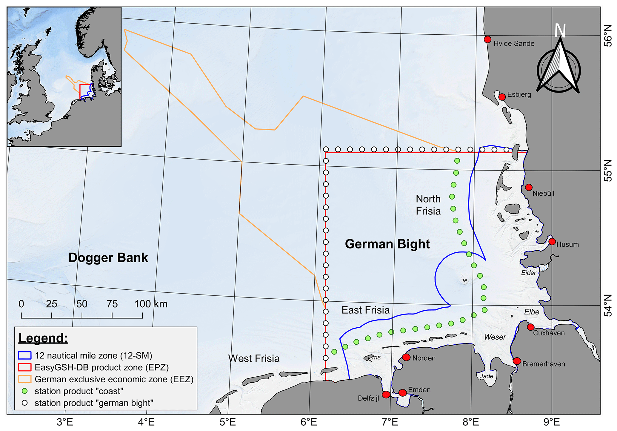
Figure 1Data product zones in the data collection. The German 12-nautical-mile zone (12-SM) is shown in blue; the EasyGSH-DB product zone (EPZ) is shown in red; and the German Exclusive Economic Zone (EEZ) is shown in orange. Green and white dots represent wave spectra results near the coast and the EasyGSH-DB product zone (EPZ).
Every item of our data collection is documented via INSPIRE-compliant metadata, including a product-specific lineage. Lineage information is an essential part of our products' metadata as it provides the option to retrieve and understand all processing steps from input data to model or analysis results (i.e., Fig. 2) and data products.
We use input data to carry out numerical modeling (i.e., simulations) to obtain unstructured model results. Either these model results are then transformed directly into data products by gridding or CSV export, or they are processed into results of tidal characteristic, statistic, or harmonic analysis. At this stage, analysis results are still unstructured and need to be converted to gridded data products. These processing steps are necessary to reduce data size, as 1 year of unstructured model and analysis results yields approximately 3.1 TB of data, while gridded data products range are in the megabyte to low-gigabyte range (15 MB to 17 GB).
All data products are distributed to users as offline (file-based) and online solutions, i.e., web map service (WMS), web feature service (WFS), or online on-the-fly web visualization via THREDDS data server (https://www.unidata.ucar.edu/software/tds/, last access: 7 June 2021).
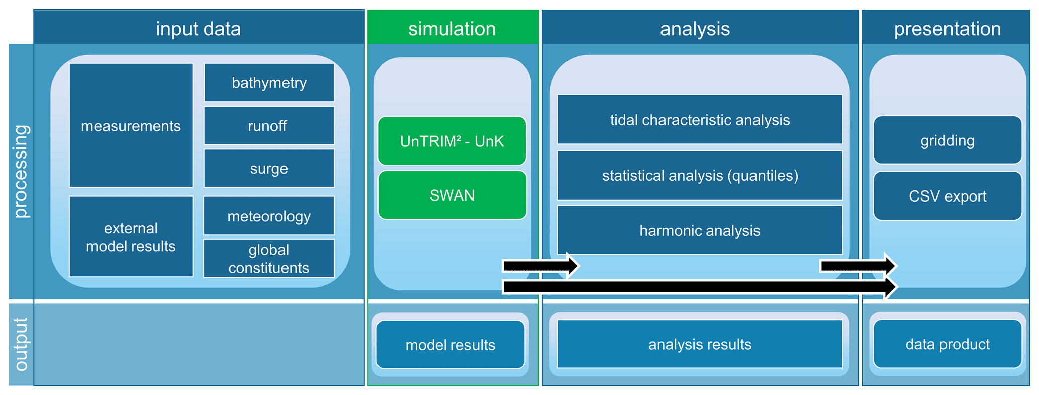
Figure 2Data product lineage (from left to right) from origin (input data), to numerical modeling (simulation), data analysis, and final presentation. The processing row indicates the data operations and tools used to produce the indicated output row. The output row defines the data state starting with unstructured modeling results followed by unstructured analysis results, and final gridded data products.
2.2 Numerical modeling
The wide range of products and data analyses require a computational model setup which (a) is consistently applicable for all 20 years, (b) is sufficiently detailed concerning horizontal and vertical mesh resolution, (c) represents all necessary physical processes, and (d) is computationally efficient. For this reason, boundary and initial data sets for water level, bathymetry, wind speed, air pressure, and freshwater discharge must be available for the entire modeling time span from 1996 to 2015 to keep data products consistent.
We apply the modeling system UnTRIM2 with the novel subgrid approach for high-resolution bathymetry representation on unstructured grids (Casulli, 1990; Casulli and Stelling, 2011) for the simulation of tidal dynamics and transport, and we apply the sediment transport module SediMorph (Malcherek et al., 2002) for bottom roughness estimation. Waves are computed by the unstructured k model UnK (Schneggenburger et al., 2000) and SWAN. The modeling approach considers 3D hydrodynamics, waves, daily freshwater discharge, hourly wind forcing and air pressure fluctuation, external surge from the North Atlantic, and the transport of salinity and heat flux. The open boundaries to the North Atlantic are forced with tidal constituents from FES2014b (FES2014 was produced by Noveltis, LEGOS, and CLS and distributed by Aviso+, with support from CNES, https://www.aviso.altimetry.fr/, last access: 7 June 2021) for astronomical water levels, constant salinity, and a characteristic monthly temperature averaged over the water column. Astronomical water level signals at the northern and southern open boundary are corrected for external surge which we incorporate by adding smoothed water level differences between calibrated simulations and nearby observations (Plüß, 2003) to the open boundary. Following this simplified approach, we take external surge and sea level rise from the North Atlantic into account. However, we imply that surge is constant along an open boundary which is not the case in nature, although modeling practice has shown that modeled sea surface agrees well with measurements in the German Bight despite this simplification. Further aspects concerning the numerical model, the calibration procedure, and a thorough validation are published separately (BAW Technische Berichte et al., 2020, in German only).
The model domain (Fig. 3) covers the North Sea from Norway to Scotland, the English Channel, and the Danish straits. Major estuaries in the German Bight, such as those of the Ems, Weser, and Elbe, are included up to their tidal weirs. The model extends approximately 1400 km in the north–south direction and 1200 km in the west–east direction. Previous modeling approaches (Heyer et al., 2015; Plüß, 2003; Putzar and Malcherek, 2015) have shown that tidal dynamics and transport in the German Bight can be reproduced well when using the entire North Sea or the entire European continental shelf (Zijl et al., 2013) as these large-scale approaches explicitly resolve tide–surge interaction and the composite amphidromic system of the North Sea.
The model uses an unstructured grid with a varying horizontal grid resolution of 10 km near the northern boundary down to 45 m in the Ems estuary, with roughly 75 % of all grid nodes located in the German Bight. The German Wadden Sea and the outer estuaries of the Ems, Weser, and Elbe are resolved with a typical edge length between 180 and 500 m (see Fig. 3 for an example of the resolution in the Wadden Sea). Additionally, a subgrid refinement is applied which improves the volume approximation of the computational grid substantially at low computational cost (Casulli, 2009; Sehili et al., 2014). The subgrid refinement ensures that the constantly varying annual bathymetry is represented in the model. Here we applied the subgrid approach with a refinement factor from 4 (open North Sea) up to 12 (within the estuaries). This discretization results in roughly 202 000 horizontal grid and 10 000 000 subgrid elements. The vertical discretization utilizes 54 fixed z layers with a half-meter resolution between +4 and −20 m NHN, gradually becoming coarser downwards.
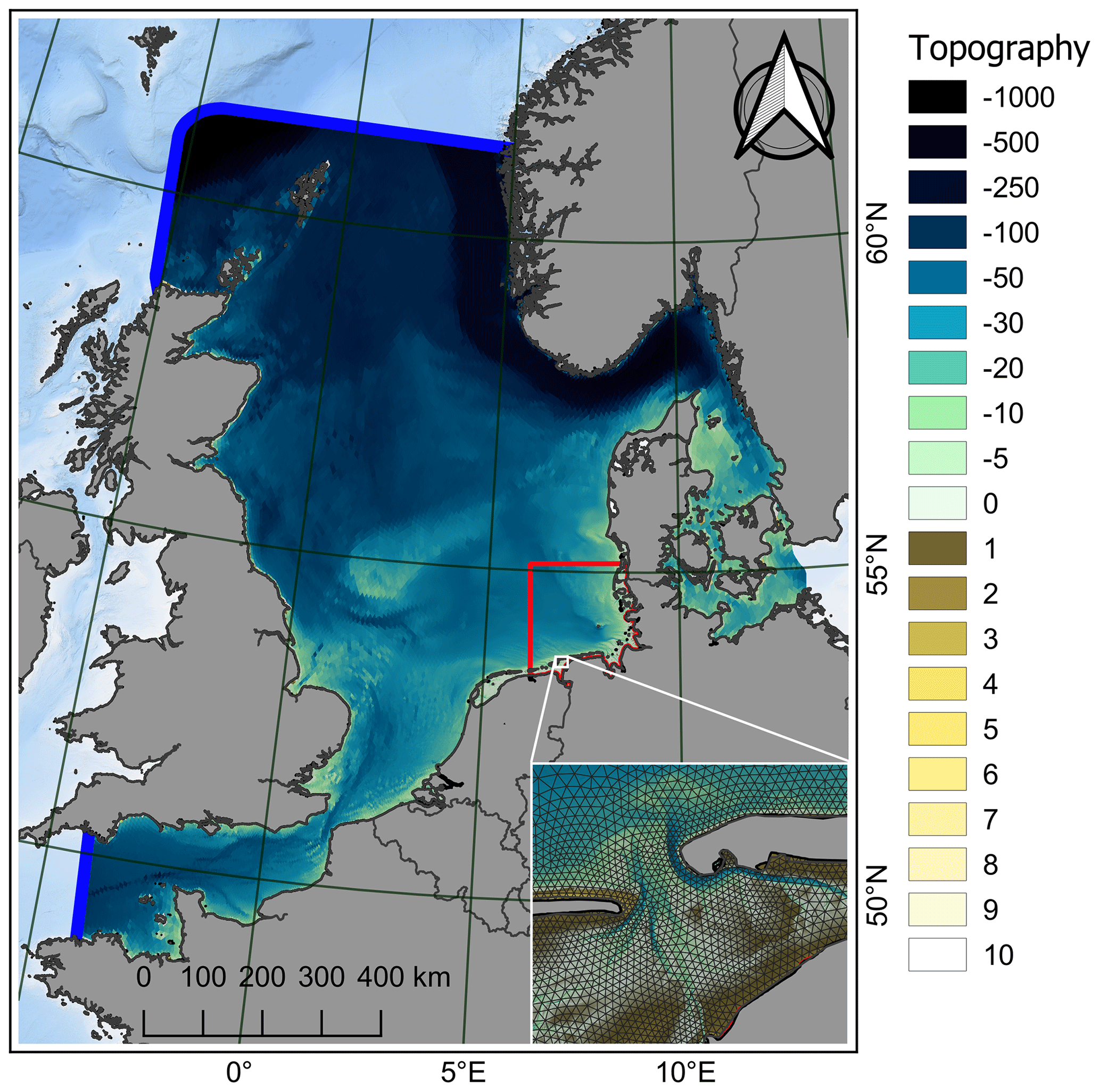
Figure 3The computational grid of the numerical North Sea model in grey, the open boundaries in blue, the EasyGSH-DB product zone (EPZ) for scale in red, and a zoom of a part of the Wadden Sea (East Frisia near the islands Juist and Norderney). Topography is given with negative values indicating depths with respect to German chart datum (m NHN).
Wind speed and air pressure fluctuation are extracted from the COSMO-REA6 data set (Bollmeyer et al., 2015) which provides hourly, reanalyzed meteorological data at a regular 6 km resolution. Freshwater discharge has been considered at the Dutch coast (the Rhine, Meuse, IJsselmeer, and Waal rivers), and for the major estuaries in the German Bight (Ems, Elbe, Weser, and Eider) together with their main confluents (Leda, Wümme, Lesum, Hunte). Dutch freshwater discharge was obtained from https://waterinfo.rws.nl/ (last access: 7 June 2021), and runoff data for the German freshwater discharge were requested from the responsible German authorities BfG, WSV, and BSH. Annual bathymetries from Sievers et al. (2021; e.g., Fig. 4) are interpolated on the computational subgrid annually within the EPZ (i.e., Fig. 1) and in parts of the Dutch Wadden Sea.
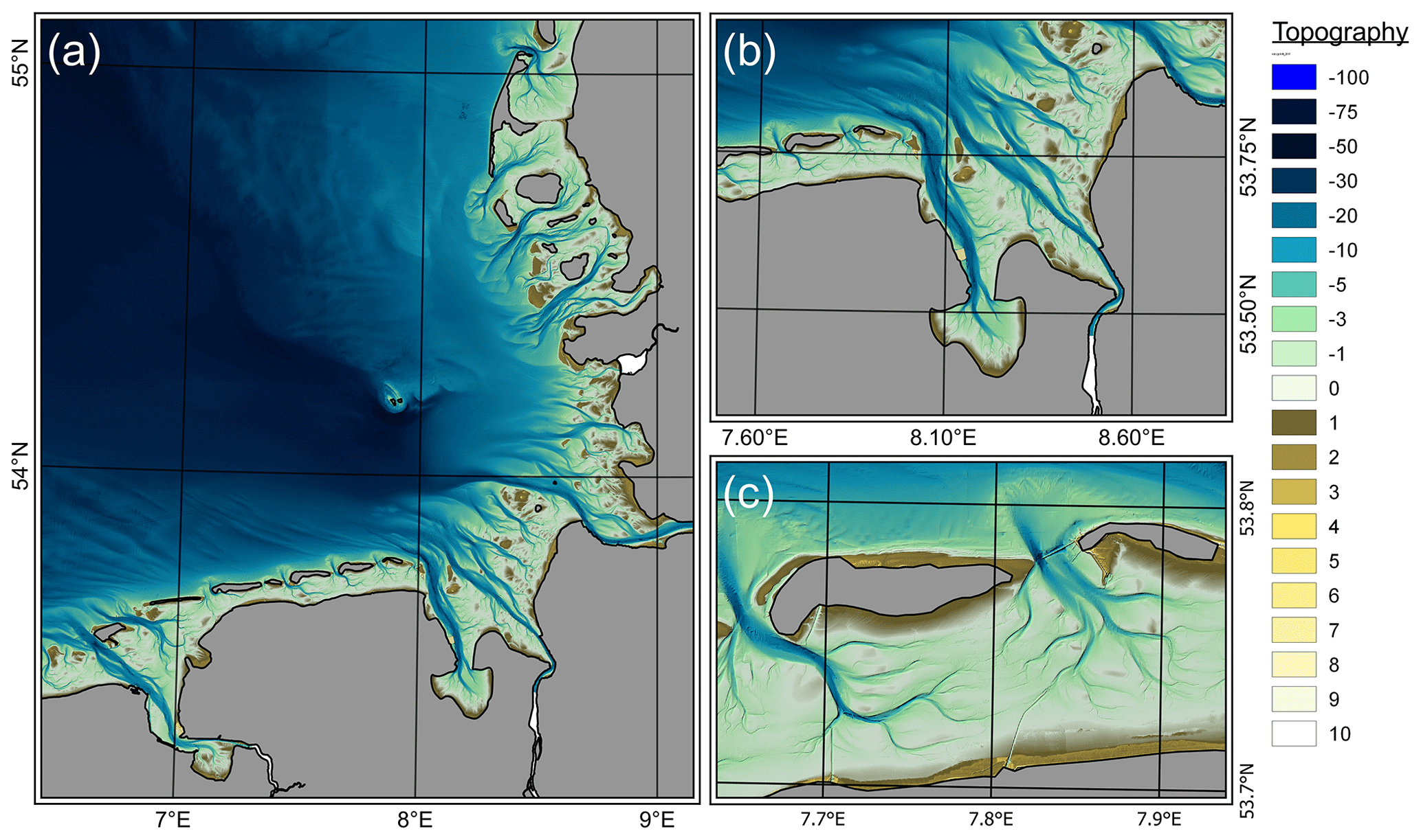
Figure 4Topography in 2015 (Sievers et al., 2020) at the native 10 m resolution in the German Bight (a), the Jade and Weser estuaries (b), and the Spiekeroog and Wangerooge inlets (c). Topography is given with negative values indicating depths with respect to the German chart datum (m NHN).
The remaining bathymetry of the North Sea was obtained from Rijkswaterstaat (https://inspire.caris.nl/viewer/, last access: 7 June 2021), UKHO (https://datahub.admiralty.co.uk/, last access: 7 June 2021), SHOM (https://data.shom.fr/, last access: 7 June 2021), and EMODnet (EMODnet Bathymetry Consortium, 2018). The bathymetry outside the EPZ was assumed to be constant over time. Data from external sources were checked semi-automatically and, if necessary, corrected for outliers and errors in units or the vertical coordinate reference system before usage.
Major groins, dams, and training walls are included in the model grid at their realistic height and extent in the German Bight. Bottom roughness has been calibrated using spatially varying Nikuradse roughness ranging from 0.08 m in the English Channel to 0.002 m in North Frisia. Turbulence closure uses a conventional k-ε model with constant values for horizontal and vertical viscosity. Initial conditions for water level, current velocity, waves, and the transport of salinity and heat are nested from model results of predecessor years. The first year (1996) was started from an astronomically forced simulation using FES2014b without a surge correction of 1995 which was initialized using the initial salinity and temperature distribution from a climatology provided by Janssen et al. (1999).
Waves are computed using the UnK and SWAN models. We chose to apply two wave models with different computational cores, physical processes, and horizontal grids to enhance the confidence in our data. The UnK wave model runs on a separate, unstructured grid which locates more (roughly 80 %) of its elements between the −30 m NHN isobath and the coastline of the German Bight. The horizontal grid resolution for waves varies between 20 km near the open boundary and 150 m in the tidal channels of the German Wadden Sea. The wave spectrum is limited to 32 frequencies between 0.006 and 1.6 Hz with 24 specified directions (steps of 15∘). UnTRIM2 and UnK are two-way-coupled which implies that the current velocity, water level, and meteorological forcing are communicated between the models at every time step. Wave energy is communicated to UnTRIM2 as wave radiation stress affecting local currents. This online coupling of a wave and hydrodynamic module improves, e.g., the prediction of water levels during storm events (Staneva et al., 2016) and currents in the shallow areas of the German Bight. A shortcoming of the UnK model is that it neglects several important physical processes, such as white capping, wave breaking, triads, or quadruplets.
For this reason, nonstationary wave simulations with SWAN are carried out on an unstructured grid which consists of 580 000 elements with 300 000 nodes in total and applies the same boundary data as the UnTRIM2–UnK modeling approach at mean water level. The model domain includes the area shown in Fig. 3 with a similar resolution from 50 m at the coast to 400 m near the −20 m NHN isobath in the German Bight and up to 2500 m in the open North Sea. Due to the absence of the water level and current interaction and therefore lower computational cost, it was possible to use a more detailed discretization of the wave spectrum. Wave spectra are resolved in 144 directions (2.5∘) using 42 frequencies (0.02 to 1 Hz). The wave model accounts for exponential wave growth due to wind exposure (Komen and Hasselmann, 1984; Hasselmann et al., 1973), white capping (Komen and Hasselmann, 1984), depth-induced wave breaking (Battjes and Janssen, 1978), bottom friction (Hasselmann et al., 1973), nonlinear wave interactions at deep and intermediate water depths due to quadruplets (Hasselmann and Hasselmann, 1985), and triads (Eldeberky and Battjes, 1996).
2.3 Data analyses
Coastal engineers often reduce complex information, such as sea surface elevation or salinity signals, to meaningful, characteristic parameters (e.g., tidal range) through harmonic or tidal characteristic analysis. Tidal characteristic values define the behavior of periodic data with mean and extreme values in a tidal context, while harmonic analysis derives the amplitude and phase for predefined (tidal) frequencies from a water level or current signal. For tidal characteristic and harmonic analysis presented hereafter, the program NCANALYSE (https://wiki.baw.de/en/index.php/NCANALYSE, last access: 7 June 2021) is applied from 1 January to 31 December for each modeled year. Note that the nodal f–u correction of tidal constituents has been disabled in the harmonic analysis because of limited applicability in the German Bight (Hagen et al., 2021).
Our tidal characteristic analysis extends a classical Eulerian analysis approach by interpreting the entire model domain in a Lagrange-like way (Fig. 5). This approach is advantageous because it guarantees that every tide and every tidal parameter in the domain are related to the same event (e.g., a tidal cycle). This procedure yields consistent characteristic values even for large domains, as each tide is linked to its predecessor. Hence, the transition from local to spatial characteristic values becomes feasible. The analysis starts by identifying each tide (i.e., times of high water and low water) within a given analysis time span for a main reference position (black dot, Fig. 5). Starting from there, a phase difference (M2 constituent only) between two adjacent locations for a chain (directed graph) of additional reference positions (red dots, Fig. 5) is determined. M2 phase differences are finally converted to the approximate travel time of the tidal wave between neighboring positions. This procedure enables us to follow the same event (i.e., tidal cycle) throughout the domain by means of shifting the data analysis period originally given for the main position. Finally, the data analysis period of the nearest reference location is used to determine, e.g., high water, low water, time of high and low water, mean water level. Lagrange-like tidal characteristic analysis can be performed for sea surface elevation, depth-averaged current velocity, depth-averaged salinity, and bed shear stress by linking these parameters to the tide. In addition, quantiles can also be calculated from the tidal characteristic values of the individual tides. A harmonic analysis of the dominant semidiurnal moon tide M2 from the sea surface elevation was carried out.
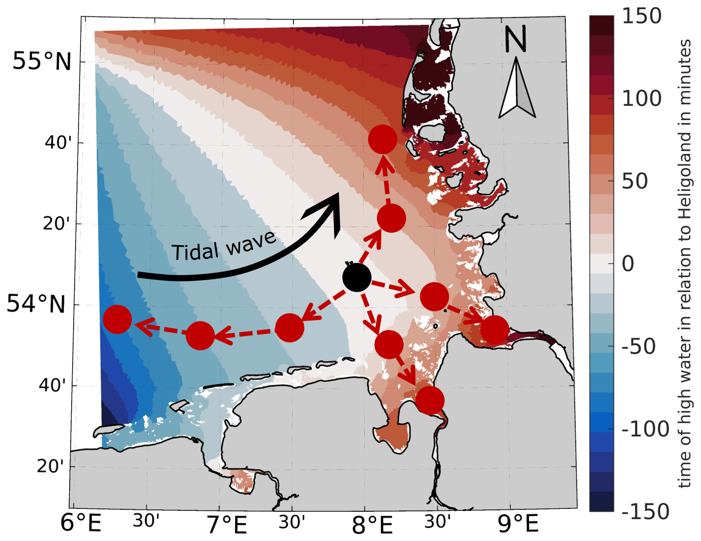
Figure 5Schematic overview of the tidal analysis methodology throughout the German Bight, showing the main reference position in black and the predecessor and successor positions in red.
Wave data analysis is performed via basic data operations, such as annual quantile or averaging, and has been carried out spatially for SWAN and UnK results.
3.1 Tidal dynamics and salinity
Figure 6 shows an exemplary hydrodynamic state with sea surface elevation in meters relative to NHN (a), north- and eastward current velocity in m/s (b), salinity in parts per thousand (c), and north- and eastward bed shear stress in N/m2 (d) on 17 November 2015, 19:00 UTC. We can see the low tide approaching from the west in East Frisia and its eastward propagation towards the mouth of the Elbe estuary (a), which results in northwestward currents at this phase of the tide (b), with current velocity above 1 m/s in the tidal channels and estuaries. The outer German Bight shows a salinity (c) between 30 and 35 ppt (i.e., g/kg), while the estuaries range between 3 and 25 ppt. Bed shear stress (d) shows seaward-directed values near the Elbe, Weser, and Ems estuaries. Bed shear stress is shown for the 12-SM zone only because, given their low amplitude, values in the deeper parts of the German Bight are negligible.
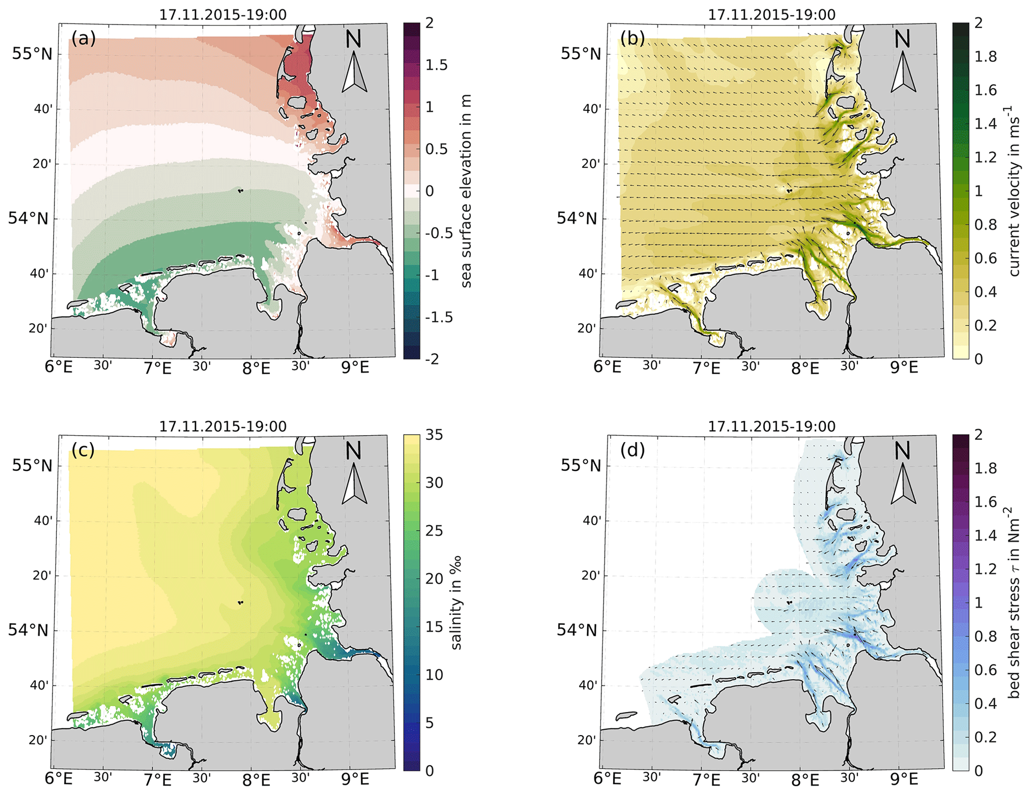
Figure 6Exemplary hydrodynamic state on 17 November 2015, 19:00 UTC, showing sea surface elevation (a), current velocity magnitude and direction (b), salinity (c), and bottom shear stress magnitude and direction (d).
The components of the hydrodynamic state (shown in Fig. 6) can be extracted at any point and time between 1 January 1996 and 31 December 2015 at the spatial and temporal resolution of the EasyGSH-DB data set of 1000 m and 20 min, respectively. It should be noted that the gridding of unstructured model results decreases data accuracy behind the islands of the Wadden Sea and in outer estuaries, because a 1 km grid is coarser than many of the narrow channels inside the Wadden Sea, resulting in a misrepresentation of wetting and drying. For this reason, the annual inundation period is supplied as an analysis product at a 100 m resolution so that cells affected by reoccurring tidal wetting and drying may be quickly identified by users. An overview of all model simulation products is provided in the Appendix as Table A1.
3.2 Waves
In Fig. 7, by way of example, gridded UnK wave products show the significant wave height Hm0, mean wave direction Θm, and peak period Tp during the storm Xaver in December 2013. Significant wave heights above 5 m are present in the deeper parts of the German Bight, and they decline quickly when reaching the nearshore areas and the Wadden Sea. UnK wave products include the significant wave height Hm0 in meters (filled contours in Fig. 7a), the mean wave period Tm02 and the peak wave period Tp (in Fig. 7b) both in seconds, and the mean wave direction Θm (vectors in Fig. 7a) and the directional spread Ψm both in degrees, in 20 min intervals.
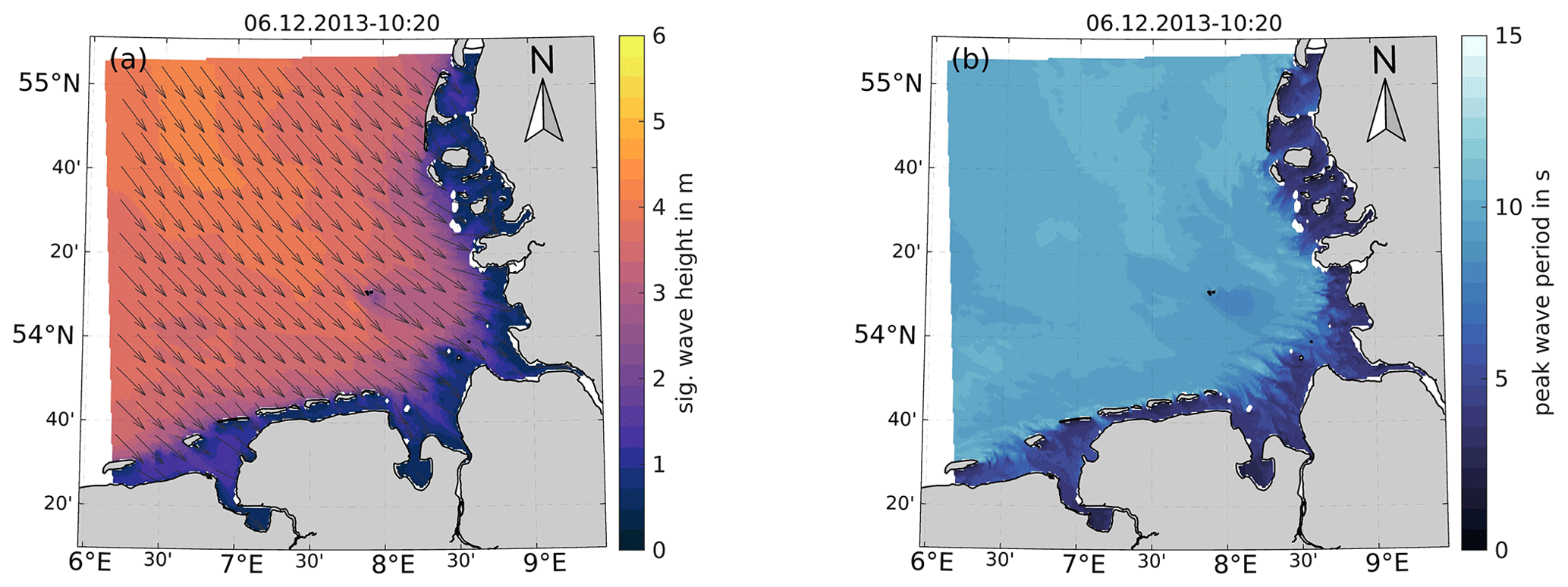
Figure 7Exemplary sea state during the storm Xaver in 2013 showing significant wave height Hm0 in meters and the mean wave direction Θm (a) and the peak wave Tp period in seconds (b) in the EPZ. Note that the mean wave direction vectors in (a) are normalized.
SWAN wave spectra are compiled at the outer boundary of the EPZ at selected locations (shown in Fig. 1, white dots). Hourly directional energy density wave spectra and time series of the wave parameters Hm0, the mean and energy wave period (Tm02 and Tm−1.0), the peak period (Tp), the mean wave direction (Θm), and directional spread (Ψm) are provided at these locations. SWAN wave spectra may be used in addition to the time series of wave parameters from SWAN or UnK, e.g., as forcing wave boundary data for numerical wave models (nesting approach) or trend analysis of wave parameters. An exemplary directional wave energy density spectrum during Xaver (at FINO1) is also provided in the Supplement, Sect. S6 to this paper.
3.3 Model data analysis
This section describes exemplary data analysis products for tidal dynamics, sea state, and salinity, which were calculated based on model results. Figure 8 shows analysis product examples of the 50 % quantile of the tidal range (a), the 50 % quantile of the ebb current velocity (b), the 50 % quantile of the tidally depth-averaged salinity (c), and the ratio of the mean flood to the mean tide depth-averaged current velocity (d) for the EPZ as annual averages of the year 2015. While the tidal range lies below 1 m at the northeast end of the German Bight due to proximity to an amphidromic point, the tidal range increases towards the coast before reaching a maximum in the Jade Bay and within the estuaries. The mean depth-averaged ebb current velocity ranges between 1 and 1.5 m/s in the deeper channels and between 0.25 and 1 m/s in the offshore areas of the German Bight. The tidally averaged and depth-averaged salinity reflects the influence of the freshwater supply from the adjacent estuaries in the German Bight, with a decrease in salinity in the mouth and downstream of the estuaries. The ratio of the mean flood to mean tide current velocity varies at a small spatial scale near the coast but indicates general flood dominance in East Frisia, which declines in the ebb delta shores of the barrier islands and the main estuaries. North Frisia demonstrates different behavior with an overall balanced ratio of flood to tide current velocity.
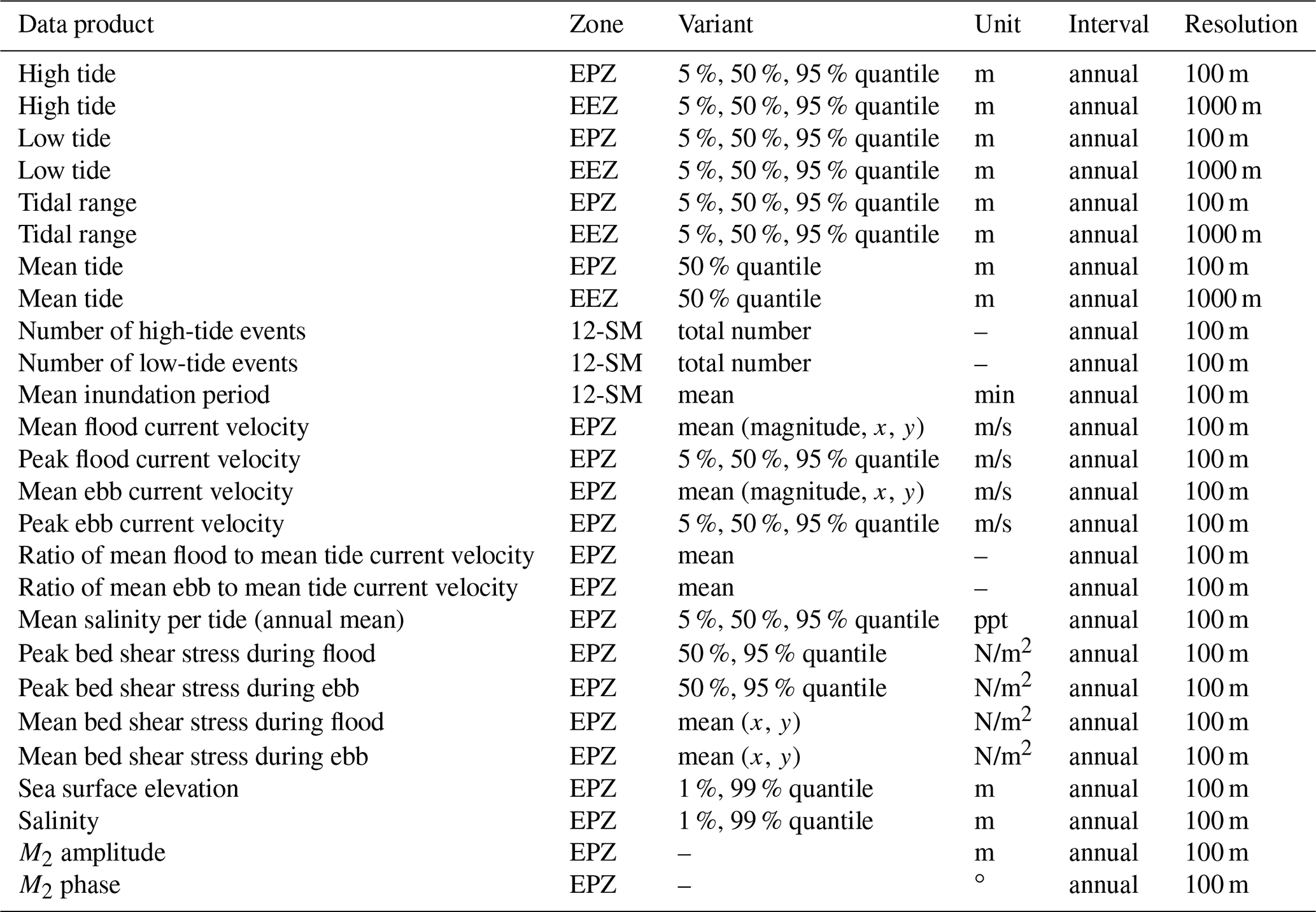
We decided to provide quantiles for scalar values and means and maxima for vector tidal characteristic values from the tidal analyses products to avoid a distortion due to, e.g., the effect of the storm surges. Extreme values for sea surface elevation and depth-averaged salinity are given by the 1 % and 99 % quantile of the annual simulation results. In addition, we provide the number of tidal high water and tidal low water events and the mean inundation period for every year. Current velocity and bed shear stress are processed accordingly. The flood-to-tide and the ebb-to-tide velocity are calculated for the quantification of current asymmetry. The harmonic analysis includes the amplitude and phase of the semidiurnal moon tide M2 (without nodal modulation; see Sect. 2.3). An overview of all analysis products is provided in the Appendix as Table A3.
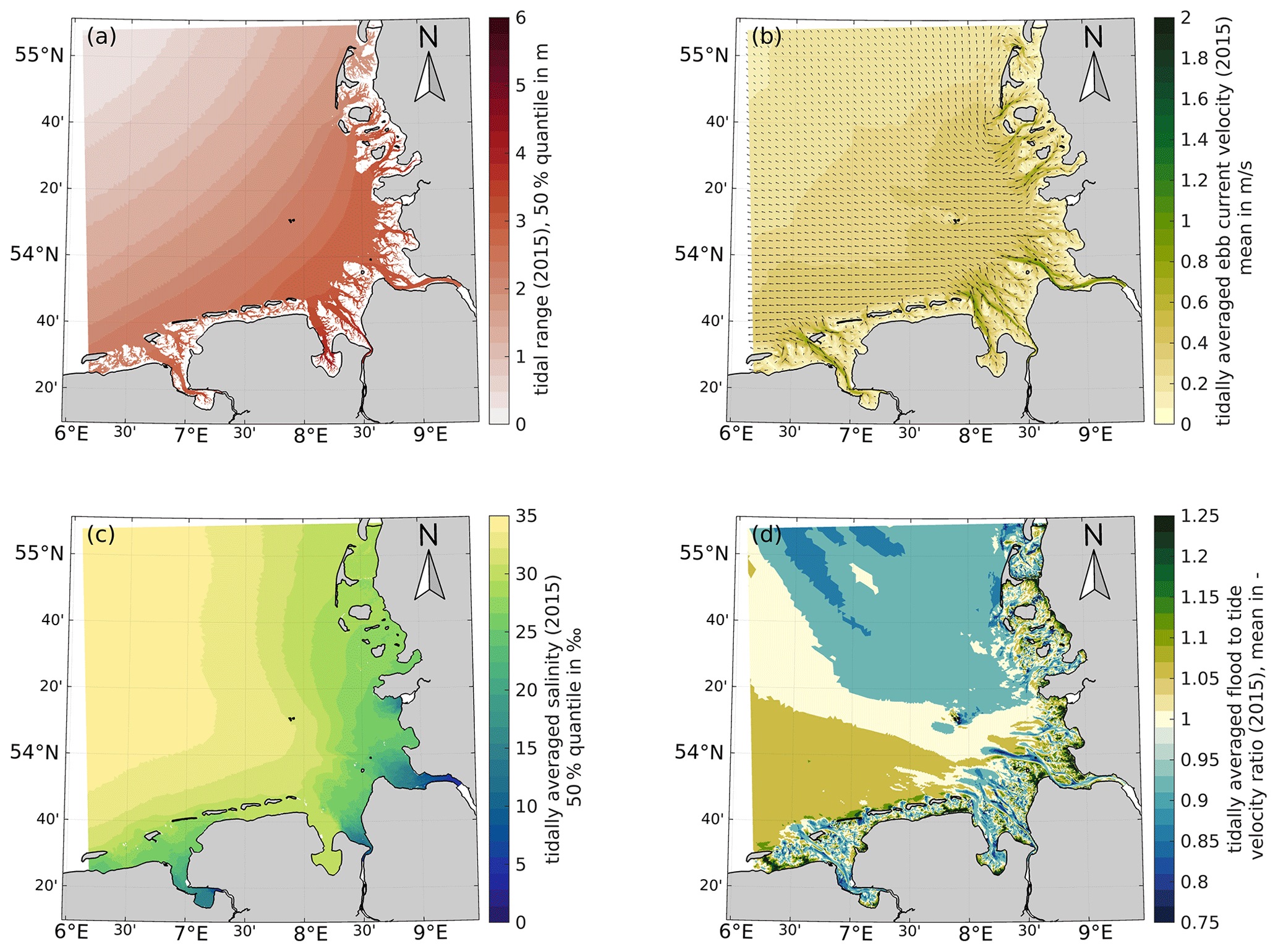
Figure 8Examples of tidal characteristic values for 2015: 50 % quantile of tidal range (a), mean tidally averaged and depth-averaged ebb current velocity (b), mean depth-averaged salinity (c), and ratio of mean flood and mean depth-averaged tidal current velocity (d).
Wave analysis products such as quantiles and the maximum of the significant wave height Hm0 and the mean wave period Tm02 at maximum significant wave height have been calculated annually for UnK and SWAN model results. SWAN products include the annual mean peak wave period, mean Hm0, mean wave energy density, a cumulative analysis of wave parameters at the “coast” and “German Bight” stations (see Fig. 1), and the energy-weighted mean wave direction (i.e., wave propagation direction as defined in IAHR, 1989) for the EPZ. Further wave analysis products have been compiled based on the SWAN simulation results at selected locations near the −20 m NHN isobath (shown in Fig. 1, green dots), e.g., for coastal protection applications. As an example, the annual combined frequency of occurrence for the significant wave height and the mean wave direction is shown for one selected location in the Supplement, Sect. S5.
In the following, we show the model's agreement with measurements for the years of 1996 to 2015 using harmonic and tidal characteristic analysis. Waves, current, and salinity are validated against measurements in the EasyGSH-DB product zone (EPZ; see Fig. 9) based on error metrics provided in the Appendix. All measurements have been checked visually and where possible corrected for outlier and suspect data points. Applied measurement locations are provided in Fig. 9. A full validation of the UnTRIM2 modeling approach is documented in BAW Technische Berichte et al. (2020) for the years 2006 and 2012. In addition, short annual validation documents (e.g., BAW Technische Berichte et al., 2019, in German only) are available for each year of our hindcast period of 1996 to 2015. Observational data were obtained from local authorities (see Sect. S1), as the marine data collection described hereafter excludes observational hydrodynamic data.
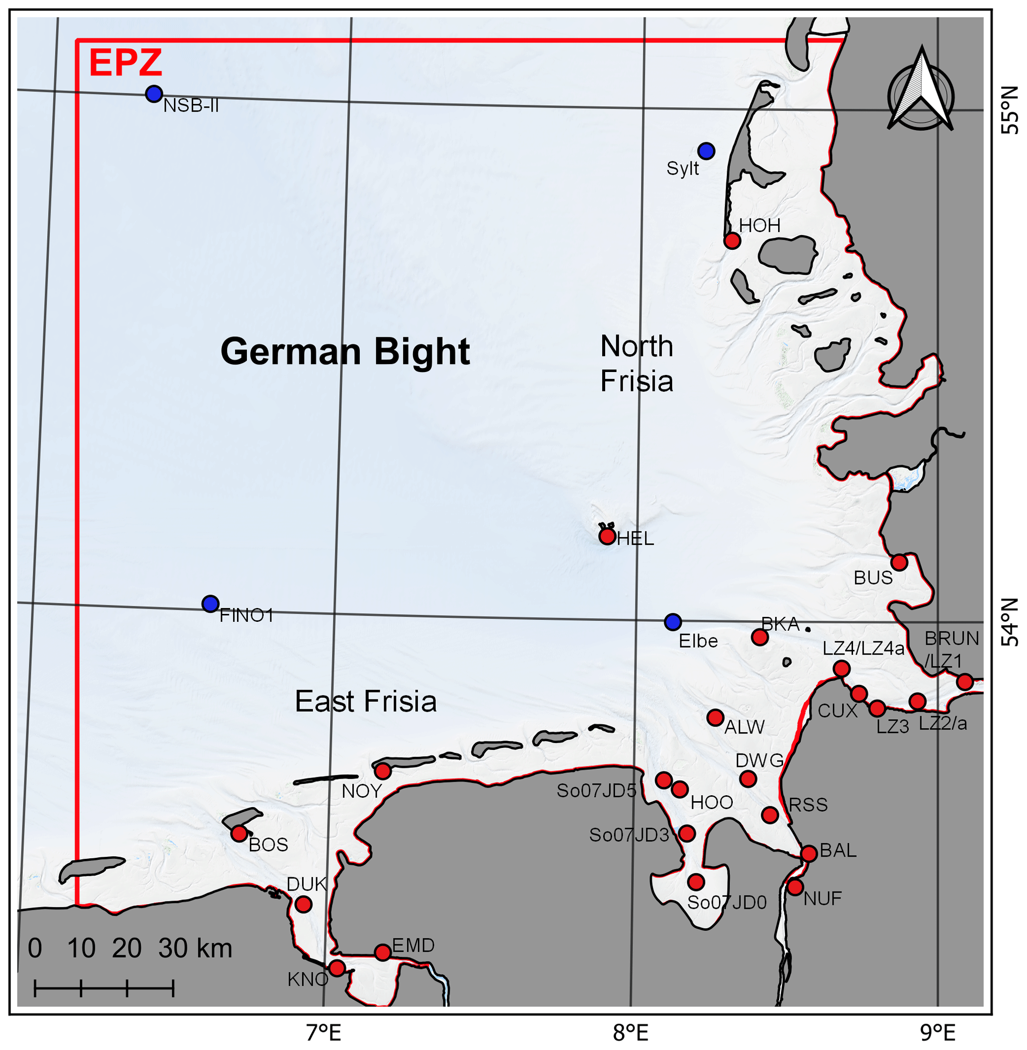
Figure 9Gauge map in the German Bight showing the gauge locations (red dots) and wave gauge locations (blue dots).
4.1 Tides
Through harmonic analysis, a water level signal can be reduced to several harmonic components with varying amplitude, phase, and frequency. As tides originate from the gravitational forces of the Sun, Moon, and Earth itself, the frequency of each driving force is clearly defined. A tidal constituent therefore represents the amplitude and phase lag of a predetermined astronomic frequency (e.g., the semidiurnal moon tide M2). The sum of all constituents is referred to as the astronomical tide, and the methodology is described extensively in literature (Codiga, 2011; Pugh, 1987). In the following, the semidiurnal moon tide M2 was chosen as its amplitude is more than 7 times larger than any other constituent in the German Bight, making it the dominant driving force of tides.
An annually varying network of 10 (1996) to 41 (2006) tide gauges in the model domain is used for validation with most gauges being inside the EasyGSH product zone (EPZ). The varying number of gauges results from limited data availability and quality restrictions of water level records. The measured and predicted water levels are analyzed harmonically (for methodology see Sect. 2.3) and the differences (errors) between predicted and observed amplitude and phase are used for error metrics. We apply a mean error (ME), a standard deviation (σ), and a root mean square error (RMSE) for a goodness-of-fit estimation of M2 amplitude and phase for each year in Table 1.
Table 1Mean error (ME), standard deviation (σ), and root mean square error (RMSE) of amplitude A in meters and phase g in degrees of the M2 tidal constituent for years 1996 to 2015. The number of gauges (No. gauges) available varies in individual years because of limited data availability and quality.
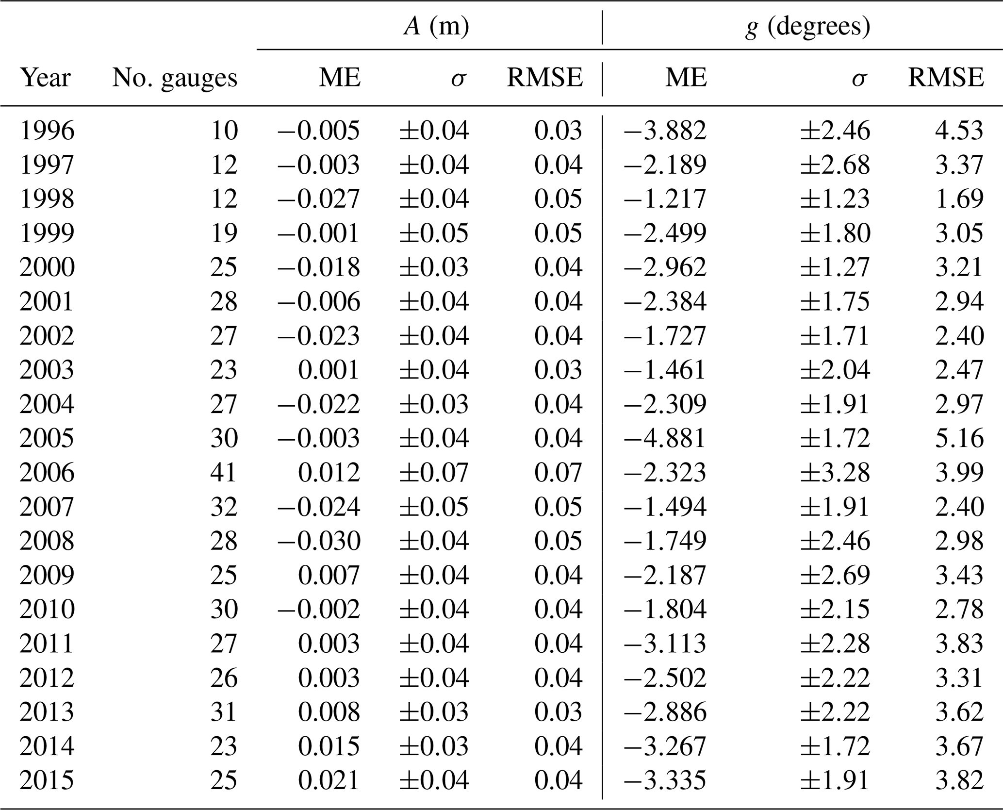
The mean error ranges between −3 and 2.1 cm with a standard deviation of 3 to 7 cm. The largest RMSE is calculated in 2006 with 7 cm and the lowest in 1996, 2004, 2013, and 2014 with approximately 3 cm. It should be noted that 2006 is the calibration year, meaning that additional gauges outside of the focus area were considered as well. The mean phase error is between −1.2 and −4.9∘ in 2005 and 1998, respectively, and the standard deviation ranges between 1.3 and 3.3∘, indicating good agreement between observation and prediction. The RMSE of the phase does not exceed 5.2∘ (2005) which would correspond to a M2 phase lag of 10 min. Comparable North Sea modeling approaches in the literature show M2 RMSEs of between 6.4 and 20 cm for the amplitude and between 5.1 and 10∘ for the phase (Gräwe et al., 2016; Jacob et al., 2016; Zijl et al., 2013; Plüß, 2003). This shows that our validation results compare well with benchmarks in the literature.
After showing in Table 1 that the model reproduces astronomical tides, we can compare observed and modeled tidal signals through their tidal characteristic values throughout the data set. Again, the RMSE is applied for each year with an average of 705 tides per year. Figure 10 displays the RMSE distribution for the tidal range at selected gauges (see Fig. 9) throughout the EPZ. If more than 50 tides per year are invalid, e.g., due to missing or inconsistent observational data, no RMSE is calculated. No-data values in Fig. 11 may therefore be explained by a lack of observed data, data gaps, a high number of suspicious values, or outliers in the measurements. The scale was chosen to a maximum of 5 % and a minimum of 1 % of a typical macrotidal range of 5 m in the German Bight.
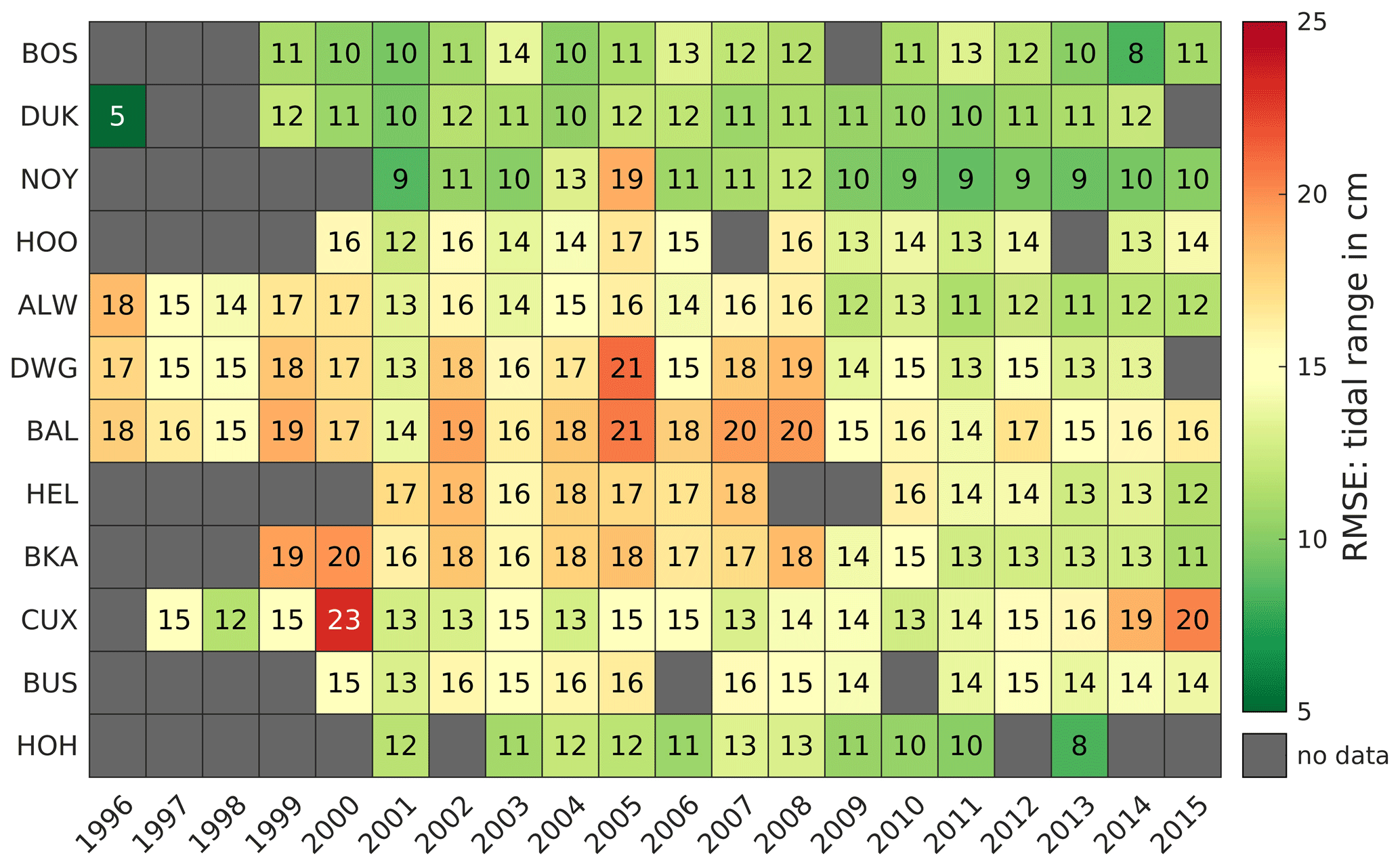
Figure 10Root mean square error (RMSE) of the tidal range in centimeters between 1996 to 2015 at representative gauges.
Most RMSEs of tidal range are between 10 and 20 cm, except for DWG, CUX, and BKA, usually before 2008. The RMSE is lowest at DUK, NOY, and HOH with 5, 9, and 8 cm, respectively, and largest at DWG, HEL, and CUX between 1996 and 2008. Large RMSE values for tide records before 2008 may be explained by uncertainty in the model bathymetry (Sievers et al., 2021) or inaccuracy of measurements caused by older, non-digital measuring instruments. As the quality improves from 2009 to 2015, the assumption that the measurement and/or the quality of the model bathymetry have improved seems most likely. In 2000, an outlier value at CUX is observed which likely results from measurement errors.
After the tidal signal has been validated for its amplitude (i.e., tidal range), the vertical extent of the signal is checked by comparing the error in the tidal high water. The comparison in Fig. 11 is structured in analogy to the tidal range in Fig. 10.
The RMSE distribution of the tidal high water shows RMSE margins of between 5 cm in HEL and 20 cm in BAL. Most RMSE values range between 7 and 13 cm. The gauges NOY, HOO, ALW, HEL, BKA, and HOH show RMSEs below 10 cm except for NOY between 2004 and 2006. The largest RMSEs are computed in DUK, DWG, and CUX, which are all tide records located in the mouths of the estuaries of the Ems, Weser, and Elbe, indicating that the error in tidal high water increases upstream of the outer estuaries. This is possibly related to an insufficient horizontal and vertical grid resolution of the numerical model in the complex bathymetry in the German estuaries.. Additionally, the gauge DWG suffers from systematic bias (not included) of 5 to 8 cm throughout all years which may also amplify its RMSE disproportionally.
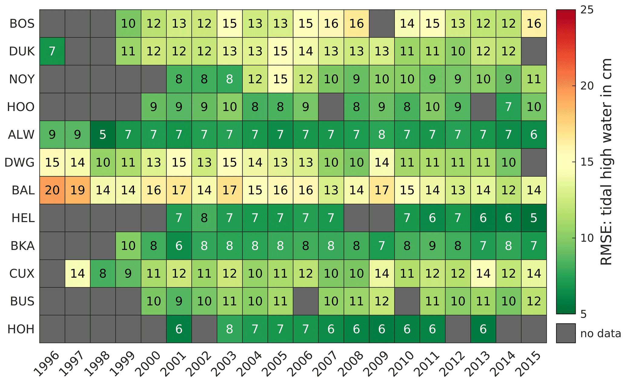
Figure 11Root mean square error (RMSE) of the tidal high water in centimeters between 1996 and 2015 at representative gauges.
The flood duration is chosen as an indicator to verify the shape of the modeled tidal signal (also asymmetry or tidal distortion). Figure 12 shows that the RMSE of the flood duration is between 10 and 20 min at most gauges. BKA, BUS, and HOH deviate with an RMSE of 20 to 37 min. While BKA and HOH show a constant deviation of 17 to 22 and 20 to 25 min, respectively, the deviation of modeled and observed data at BUS increases with time. After 2010, the error remains constantly above 29 min, which may be the result of local bathymetric changes that are not represented in model bathymetry, especially in the morphologically active Meldorf Bay near BUS. This is probable, as tidal asymmetry is strongly influenced by bathymetry (Friedrichs and Aubrey, 1988).
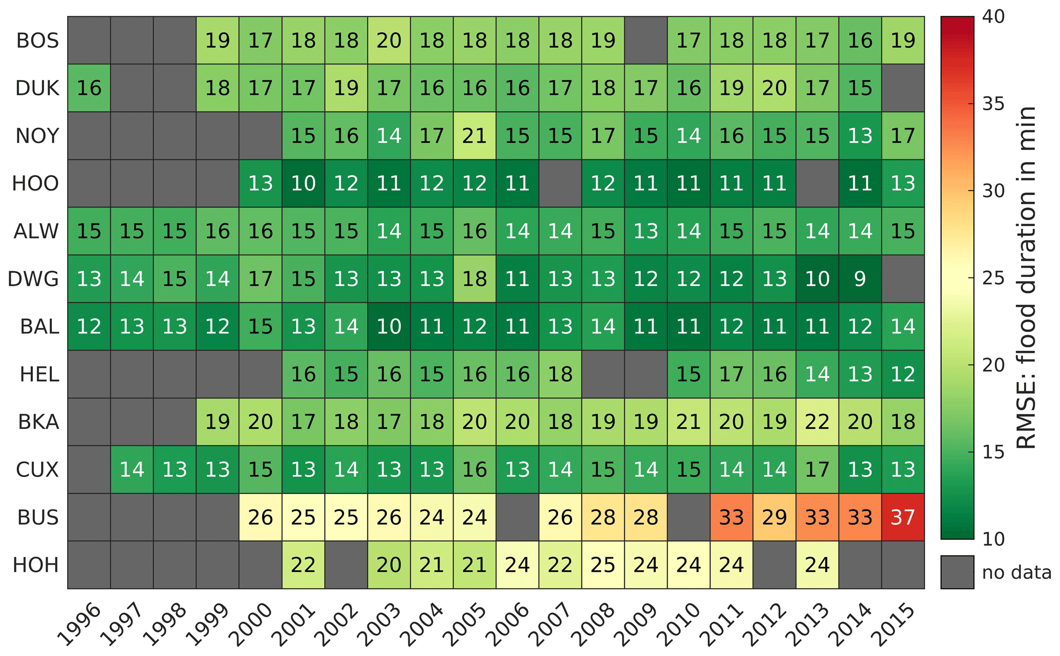
Figure 12Root mean square error (RMSE) of the flood duration in minutes between 1996 and 2015 at representative gauges.
In addition to the average high water, tidal range, and flood duration, extreme events play a role as the southern North Sea is subject to frequent storm surge events. For this reason, we evaluate extreme events by comparing the 99 % quantile of sea surface between the model and observation. Figure 13 shows that the error in the 99 % quantile is usually lower than 10 cm. The lowest error margins are observed at ALW, HEL, BKA, and BUS.
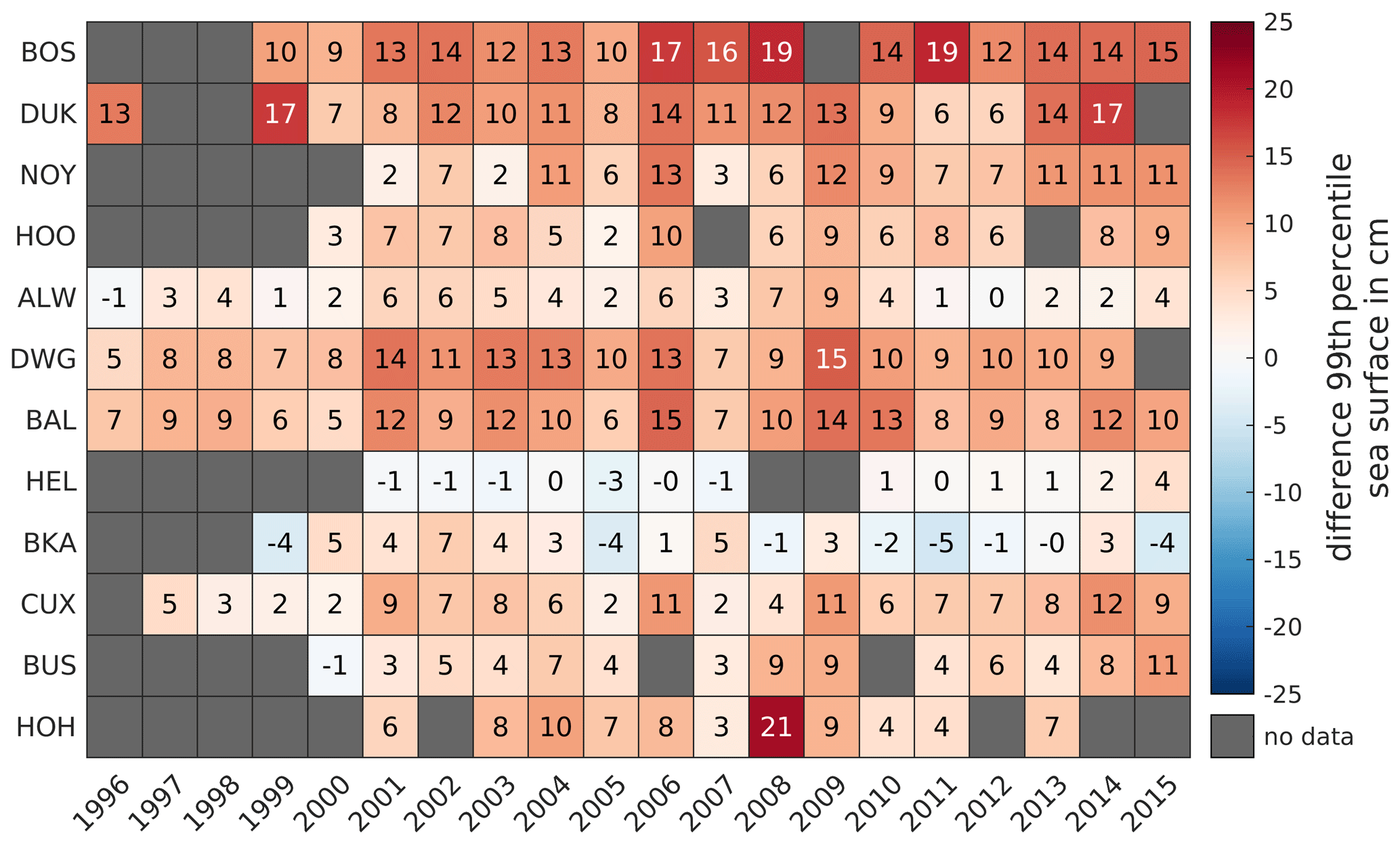
Figure 13Difference in the 99 % water level quantile in centimeters between 1996 and 2015 at representative gauges with positive values indicating water level overestimation by the model.
However, the model tends to overestimate extreme water levels in the eastern EPZ near the Ems estuary (BOS, DUK, NOY) and in the Weser estuary (DWG, BAL), which is possibly related to the estuarine location of these gauges. Errors range from a maximum overestimation of 21 cm in HOH (outlier) to an underestimation of −4 cm at BKA. Hence, our model data slightly overestimate extreme water levels in the EPZ in the order of centimeters to tens of centimeters.
4.2 Current velocity
The uncertainty in current velocity measurements (van Rijn et al., 2000) and the sensitivity of computed current velocities to water depth and water depth gradients have a strong impact as they limit the comparability of observed and modeled current velocity. Nevertheless, we have carried out a validation of current velocity magnitude for available data in the Ems, Elbe, and Jade estuaries (Fig. 14) with a statistical approach, to account for the limited possibility of a direct comparison. For the purpose of validation, model data have been extracted at the depths of measurement devices. Samples are colored in the plots according to sample density. Moreover, the index of agreement R2 and a linear regression with the slope m and the y intercept b are used to obtain information about bias or time lag. The y intercept b is an indicator for bias, and the slope m is an indicator for potential phase lag (Winter, 2007).
R2 varies between 0.49 and 0.89, indicating a high correlation between the predicted and observed current velocity magnitude. Comparisons at LZ1 and LZ4 show R2 values of less than 0.51, which is due to a wider spread in the measured velocity data in the river Elbe in the year 2012. Thus, the regression parameters demonstrate cases of poor agreement as well. Model skill in the Ems and Jade estuaries (a–c, f), however, shows strong agreement between prediction and observation, although low regression slopes below 0.77 are found in So07JD0, LZ1, LZ4, and KNO, indicating a slight offset in the velocity signal between flood and ebb.
More information on the direction of current velocities is given by hodographs (provided in Sect. S2) of the current velocity at LZ1 and LZ4. They show that measured current velocity varies more in the north- and southward direction at LZ1, even though most of the ebb and flood peak currents are well reproduced by the model. The hodograph in LZ4 reveals that the model underestimates the ebb and flood current as well as the cross-channel velocity variation. This is likely related to strong three-dimensional effects at this location and to issues with measurement quality at high current velocity magnitudes.
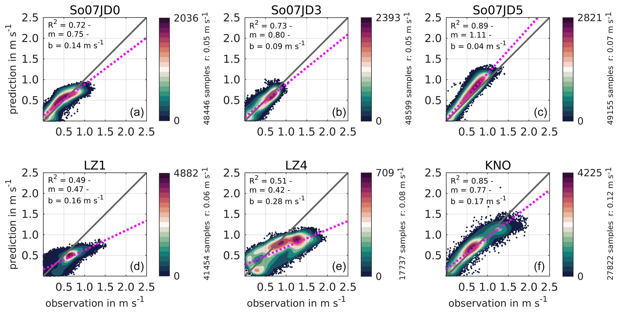
Figure 14Scatterplots of current velocity magnitude at different gauges in the German Bight in 2012: in So07JD0 (a), So07JD3 (b), and So07JD5 (c) in the Jade estuary; in LZ1 (d) and LZ4 (e) in the Elbe estuary; and in KNO (f) in the Ems estuary. Figures are colored according to sample density and contain the index of agreement R2 as a measure for regression quality and the linear regression slope m and y intercept b in m/s. The dotted pink line represents a linear regression, and the solid black line represents an optimal correlation between observation and prediction.
4.3 Salinity
Salinity is validated at different gauges between 1997 and 2015 in analogy to Sect. 4.1. The year 1996 is neglected due to the absence of observational data. We apply the RMSE for the observed and predicted salinity in Fig. 15. No-data values result from limited availability of observations to the authors, inconsistent data quality and quantity, or bias in the observational data sets. We have focused on estuarine gauges as these demonstrate the highest salinity variation due to freshwater discharge. Nevertheless, it was possible to achieve a solid spatial and temporal coverage in the German Bight. It should be noted that error margins for the RMSE of salinity depend on the amplitude of salinity fluctuation during a tidal cycle, which is why RMSEs are typically lower outside the estuary brackish-water zones.
RMSE values in Fig. 15 vary between 0.7 and 4.5 ppt, although most RMSEs are in the range between 1 and 3 ppt. The best overall agreement is found at NUF and ALW, which are situated in the inner and outer Weser estuary, while the worst agreement is found at KNO (in 2000) in the Ems estuary and at LZ4 in the mouth of the Elbe estuary. Nearby gauges (e.g., LZ3 or LZ4a), nevertheless, demonstrate lower RMSE values, which makes a slight vertical or horizontal misplacement in the model for LZ4 probable.
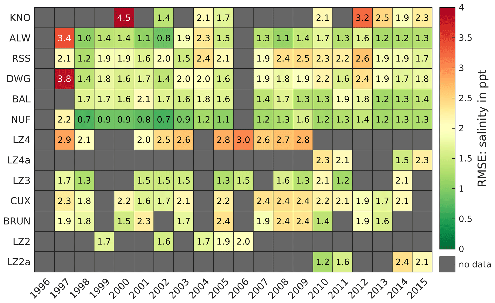
Figure 15Root mean square error (RMSE) of the salinity in parts per thousand between 1996 and 2015 at representative gauges.
4.4 Waves
We compare SWAN and UnK wave model results (significant wave height Hm0, mean wave period Tm02, peak period Tp, and mean wave direction Θm) against wave measurements in the German Bight by computing the RMSE. Wave measurements in the EasyGSH-DB product zone (EPZ) suffer from low data availability in contrast to, e.g., water level measurements. Most wave measurements in the EPZ were recorded in short-term measuring campaigns covering a few years at best. Hence, we decided to assess model performance for the product time span at a few locations only. Due to data gaps in measurements, it is impossible to validate every model time step within a year. Therefore, we provide an annual completeness of the measured significant wave height in Table 2. Completeness hereby refers to the number of valid measurement samples at model output times divided by the total number of model output times. Measurements were checked visually for credibility and outliers, and suspect points were deleted. As mentioned before in Sect. 2.2, local water levels and current interaction are neglected for SWAN simulations. Thus, the validity of these results is limited to deep water conditions (i.e., areas with water depths of smaller than −20 m NHN). Swell wave events from the North Atlantic are not captured by our model setup which does not consider open-boundary wave forcing along the ocean model boundary. Therefore, we observe an underestimation of peak wave periods during calm-weather conditions in the study area.
Table 2 outlines wave validation results for a chosen year 2007 at the stations FINO1, Sylt, Elbe, and NSB-II (see Fig. 9). All stations show limited completeness, between 89 % at Elbe and only 25 % at NSB-II. Deep sea measurements (FINO1, NSB-II) demonstrate lower RMSE values with SWAN, while nearshore samples (e.g., Sylt, Elbe) show better agreement from the two-way wave–current coupling of UnTRIM2 and UnK. Both models represent the significant wave height well at all stations with a maximum RMSE of 0.74 in NSB-II (UnK). The RMSE of Tm02 and Tp remains within 3.22 s for both approaches, even though SWAN demonstrates a lower RMSE for wave periods. Mean wave direction displays RMSE values of between 37.9 and 54.4∘, although it should be noted that mean wave directions from simulation results are compared with measured wave direction at the peak frequency. These two values differ episodically, which is a likely explanation for low model skill. Analogous to the RMSE of significant wave heights, there are larger deviations when comparing intermediate water depths (e.g., Sylt in Table 2) due to the applied mean water level and the fact that the SWAN modeling approach does not account for current interaction. As a result, nearshore wave refraction is inaccurate.
Table 2Root mean square error (RMSE) of the significant wave height (Hm0), mean wave period (Tm02), peak wave period (Tp), mean wave direction (Θm), water depth (d), and completeness of the measured significant wave height at selected locations for the year 2007.

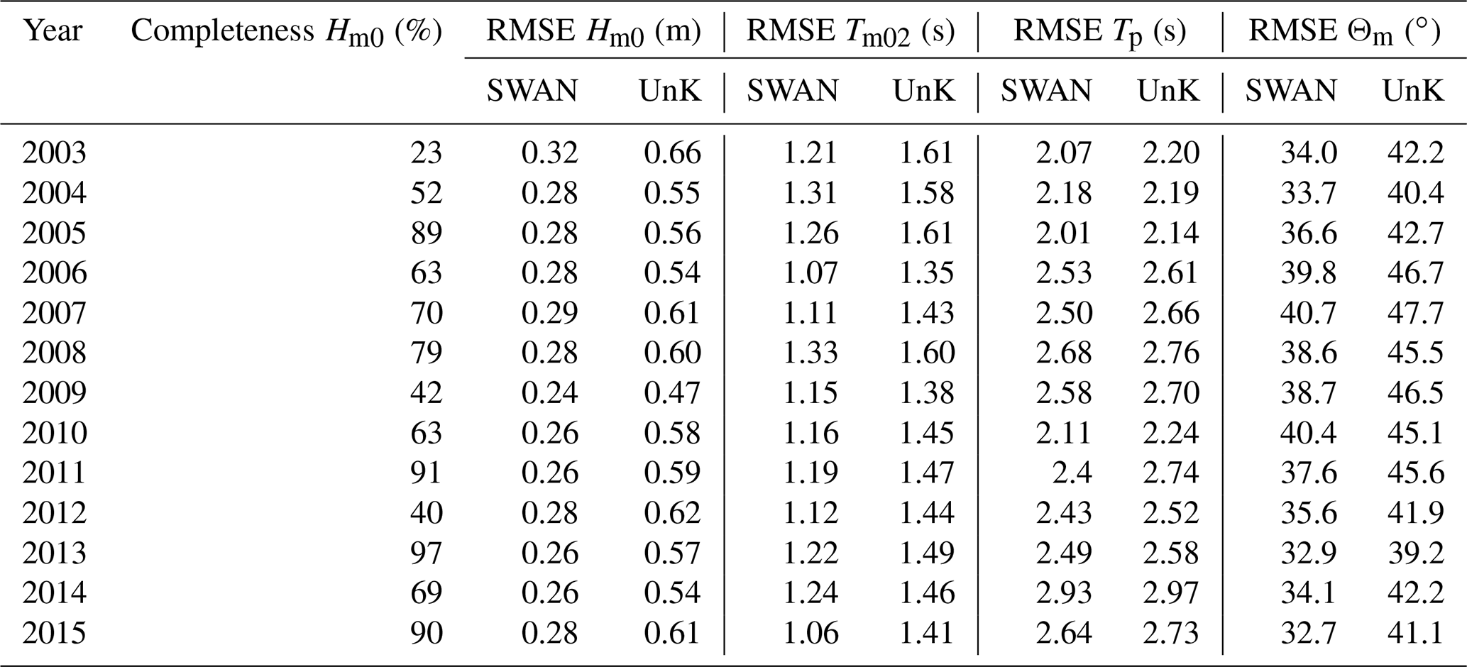
Table 3 shows an assessment of the simulated significant wave height, mean wave period, peak wave period, and mean wave direction and available measurements at FINO1 (open sea research platform about 45 km to the north of the East Frisian island of Borkum; see location in Fig. 9; operational since July 2003) for the years 2003 to 2015. Analogous results at Elbe and NSB-II are provided in Sects. S3 and S4 for the sake of completeness.
The annual RMSE of the significant wave height near the location of FINO1 ranges between 0.24 and 0.32 m for the SWAN and between 0.47 and 0.66 m for the UnK model results. RMSE values are on the same order for other locations in deeper water. Nevertheless, slightly differing RMSE values are observed for the locations Elbe and NSB-II, as larger deviations occur in areas with intermediate water depths (e.g., RMSE near the location Sylt in Table 2) due to current interaction which leads to better skill in the fully coupled UnTRIM2–UnK simulations. The mean wave period is systematically underestimated in both wave simulations. This phenomenon is known from comparisons of measured and calculated wave spectra from wave hindcasts in the western Baltic Sea (Schlamkow and Fröhle, 2008) and was related to the wind energy input formulation applied in SWAN. The annual RMSE of the mean wave period at FINO1 ranges between 1.07 and 1.33 s (SWAN) and between 1.35 and 1.61 s (UnK). The RMSE of the peak period at FINO1 varies between 2.07 and 2.93 s (SWAN) and between 2.14 and 2.97 s (UnK). Differences >12 s between observed and modeled peak periods possibly arise from neglecting open boundary wave conditions at the North Atlantic in the model setup or from differences between the observed and applied wind field. Moreover, the reliability of measurements for peak periods >12 s with a directional wave rider buoy, such as FINO1, remains questionable. Hence, outlier differences with respect to the peak period may be related to a coarse measurement resolution of long wave periods and wave spectra. For reasons explained above, the annual RMSE of the mean wave direction at FINO1 is between 33.7 and 40.7∘ (SWAN) and between 40.4 and 47.7∘ (UnK).
Considering our validation results, we suggest applying UnK wave data for coastal applications because of the sea surface and current interaction, while SWAN results are suited for nesting approaches in the German Bight due to their high directional and spectral resolution.
Table 3RMSE of significant wave height (Hm0), mean wave period (Tm02), peak wave period (Tp), mean wave direction (Θm), and measured Hm0 completeness from 2003 to 2015. Note that FINO1 started operating in July 2003, which is why no earlier RMSEs are available.
Open-access EasyGSH-DB data products (Hagen et al., 2020a, b) can be obtained separately in two categories for hydrodynamic analyses (https://doi.org/10.48437/02.2020.K2.7000.0003) as GeoTIFF and ESRI shape files and hydrodynamic simulation results (https://doi.org/10.48437/02.2020.K2.7000.0004) in a common structured NetCDF format. Stationary wave products count within the simulation result category and are available in ASCII format for further processing or direct nesting. EasyGSH-DB data can be obtained by download and via web services (YYYY translates to 1 year between 1996 and 2015):
-
web map service (WMS; http://mdi-dienste.baw.de/geoserver/EasyGSH_Kennwerte_YYYY_/wms, last access: 7 June 2021),
-
web feature service (WFS; http://mdi-dienste.baw.de/geoserver/EasyGSH_Kennwerte_YYYY_/wfs, last access: 7 June 2021),
-
web coverage service (WCS; http://mdi-dienste.baw.de/geoserver/EasyGSH_Kennwerte_YYYY_/wcs, last access: 7 June 2021).
An overview of products, publications, and web services can be found on the EasyGSH-DB website (https://mdi-de.baw.de/easygsh/, last access: 25 April 2021). Users can view, animate, and explore data through interactive web map viewers. All data are under the Creative Commons license 4.0 (CC-BY 4.0).
The presented integrated marine data collection for the German Bight for the period from 1996 to 2015 establishes a reliable, high-resolution database of hydrographical parameters for scientific, commercial, and governmental organizations. Based on the involvement and participation of coastal stakeholders, hydrodynamic model results (i.e., sea surface elevation, depth-averaged current velocity, bed shear stress, depth-averaged salinity, wave parameters) are provided as files and online on a 1000 m grid in the German Bight with 20 min time intervals. Additionally, analysis products (tidal characteristic values, e.g., tidal range, flood current velocity, significant wave height) have been created from simulation results to improve the accessibility of this data set and to reduce data size. Data products are extensively validated and can be used for various applications in oceanography, Earth sciences, and coastal engineering, although the limitations defined in this report must be considered before application.
The numerical modeling approach aims to provide a synthesis of consistent forcing parameters (e.g., freshwater discharge, wind speed, and tidal dynamics) and geomorphology. Annually updated geomorphology is a unique feature of this data collection compared to previous studies which have mainly considered static bathymetry over short and long time spans. By using the same basic assumptions concerning grid configuration and resolution, numerical parameters, friction height, surge assimilation, and wind forcing as well as freshwater discharge for 20 years, this investigation produces a homogeneous, consistent data set. The collection can therefore serve as the starting point for more detailed simulations in the German Bight to further increase our understanding of the complex dynamic processes combining geomorphology and hydrodynamics. The early involvement of potential stakeholders has shown potential uses apart from scientific applications. The range of applications covers coastal engineering projects such as the planning of offshore wind farms to support environmental tasks or the description of habitats for the European Marine Strategy Framework Directive. From a scientific perspective, consistent, long-term tidal characteristic values are not a novel concept, but scientific practice has shown that their application is advantageous, even though they are not commonly used. In Sect. 4, we have touched upon the potential for describing the ability of a model to reproduce the main tidal properties of a large area over long timescales, using only a few tidal characteristic parameters.
Although the marine data collection already covers a time span of 20 years, this period is still too short for many applications (e.g., studying the effect of a rise in mean sea level). Therefore, a continuous extension of the data collection from 2016 onwards would be desirable. An extension to the past also seems conceivable, yet it must be noted that the quality of input forcing data decrease drastically before 1996. Finally, we emphasize that any modeling approach critically depends on the availability of international field data, especially for the ever-changing bathymetry, measurements for validation, and open boundary as well as initial forcing data. This stresses the immediate need for international mutual databases, minimum quality standards, good scientific practice to reduce data clutter, and complete INSPIRE-compliant metadata.
A1 Error metrics
To describe the quality of a model, an error threshold must be specified. An error Et in model validation concerns the difference between observed (O) and predicted (P) values (or vice versa). The mean error (ME; Eq. A1) is the arithmetic mean over the difference in observed and predicted values for N samples at mutual time t. The standard deviation σ (Eq. A2) describes the error spread of the error distribution around the mean error with μ being the mean of all Et.
The root mean square error (RMSE; Eq. A3) takes the root of the mean squared errors Et. The squaring of differences weighs the RMSE towards larger error margins. It should be noted that any information about over- or underestimation is lost due to the application squared errors.
The coefficient of determination R2 is defined as an indicator of the proportion of the sum of squares of data explained by a regression model in percent. Hence, the closer R2 is to 1, the better the fitted data are explained by a regression model.
A2 Product list
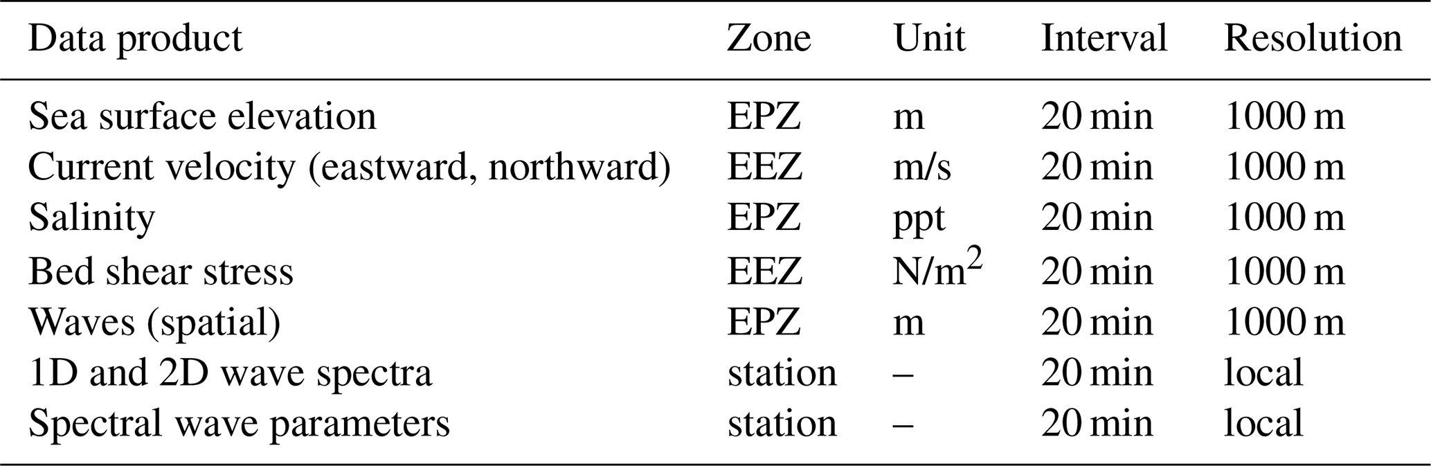
Table A2Wave analysis products divided by the simulation software UnK and SWAN.
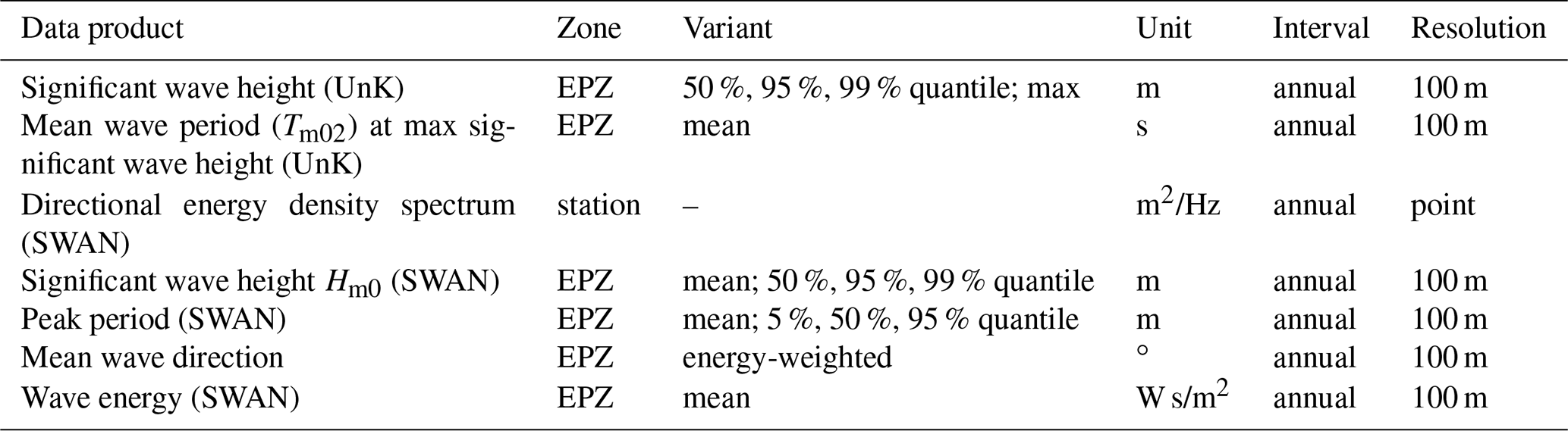
Table A3Tidal characteristic and harmonic data analysis products.
The supplement related to this article is available online at: https://doi.org/10.5194/essd-13-2573-2021-supplement.
RH contributed to article composition, article figures, article concept, numerical modeling of UnTRIM2–UnK, validation of UnTRIM2, conceptual product design, and lineage design. AP contributed to project initiation, supervising, proofreading, conceptual product design, and lineage design. RI contributed to metadata and repository management and digital object identifier registration. JF contributed to model result processing and tidal characteristic, statistic, and harmonic analysis. ND contributed to numerical modeling of SWAN, model result processing and analysis (SWAN waves), validation of SWAN, and proofreading. EN contributed to supervising, proofreading, and lineage design. NiS contributed to numerical modeling of SWAN (grid composition), model result processing and analysis (SWAN waves), and lineage design. PF contributed to project initiation, supervising, and proofreading. FK contributed to project initiation, supervising, proofreading, and the article concept.
The authors declare that they have no conflict of interest.
The authors thank the German Federal Ministry of Transport and Digital Infrastructure (BMVI) for funding the mFUND project EasyGSH-DB (funding no. 19F2004A-D), which has made this data collection possible. We also thank the suppliers of field measurements we used to validate our numerical models (i.e., Sect. S1). We would like to express our gratitude to all EasyGSH-DB collaborators, i.e., smile consult GmbH, Küste und Raum, and the German Federal Maritime and Hydrographic Agency (BSH), for their valuable input and collaboration which we enjoyed. We recognize thankfully the input of the two anonymous reviewers, who have helped us to improve our manuscript significantly. Also, we would like to acknowledge the many stakeholders and beta testers who have provided constant feedback and contributed their time to improve our data products presented herein. The BAW authors furthermore wish to express their gratitude to the PROGHOME team for excellent software solutions and extraordinary support at a very high level. Robert Hagen and Janina Freund thank Günther Lang for his important input towards the description of the analysis methodology.
This research has been supported by the Bundesministerium für Verkehr und digitale Infrastruktur (grant no. 19F2004A-D).
This paper was edited by Giuseppe M. R. Manzella and reviewed by two anonymous referees.
Battjes, J. A. and Janssen, J. P. F. M.: Energy loss and set-up due to breaking of random waves, Coastal Eng., 1978, 569–587, https://doi.org/10.1061/9780872621909.034, 1978.
BAW Technische Berichte, Hagen, R., Freund, J., Plüß, A., and Ihde, R.: Jahreskennblatt 2015, BAW Technischer Bericht B3955.02.04.70229.1, Bundesanstalt für Wasserbau, https://doi.org/10.18451/k2_easygsh_jkbl_2014, 2019 (in German).
BAW Technische Berichte, Hagen, R., Freund, J., Plüß, A., and Ihde, R.: Validierungsdokument EasyGSH-DB Nordseemodell. Teil UnTRIM2 – SediMorph – UnK, BAW Technischer Bericht B3955.02.04.70229.1, Bundesanstalt für Wasserbau, https://doi.org/10.18451/k2_easygsh_1, 2020 (in German).
Benninghoff, M. and Winter, C.: Recent morphologic evolution of the German Wadden Sea, Sci. Rep.-UK, 9, 9293, https://doi.org/10.1038/s41598-019-45683-1, 2019.
Bollmeyer, C., Keller, J. D., Ohlwein, C., Wahl, S., Crewell, S., Friederichs, P., Hense, A., Keune, J., Kneifel, S., Pscheidt, I., Redl, S., and Steinke, S.: Towards a high-resolution regional reanalysis for the European CORDEX domain, Q. J. R. Meteor. Soc., 141, 1–15, https://doi.org/10.1002/qj.2486, 2015.
Casulli, V.: Semi-implicit finite difference methods for the two-dimensional shallow water equations, J. Comput. Phys., 86, 56–74, https://doi.org/10.1016/0021-9991(90)90091-E, 1990.
Casulli, V.: A high-resolution wetting and drying algorithm for free-surface hydrodynamics, Int. J. Numer. Meth. Fluids, 60, 391–408, https://doi.org/10.1002/fld.1896, 2009.
Casulli, V. and Stelling, G. S.: Semi-implicit subgrid modelling of three-dimensional free-surface flows, Int. J. Numer. Meth. Fluids, 67, 441–449, https://doi.org/10.1002/fld.2361, 2011.
Codiga, D.: Unified tidal analysis and prediction using the UTide Matlab functions, URI/GSO Technical Report 2011-01, 61 pp., 2011.
Eldeberky, Y. and Battjes, J. A.: Spectral modeling of wave breaking: Application to Boussinesq equations, J. Geophys. Res., 101, 1253–1264, https://doi.org/10.1029/95JC03219, 1996.
EMODnet Bathymetry Consortium: EMODnet Digital Bathymetry (DTM 2018), EMODnet Bathymetry Consortium, 2018.
Friedrichs, C. T. and Aubrey, D. G.: Non-linear tidal distortion in shallow well-mixed estuaries: A synthesis, Estuarine Coast. Shelf Sci., 27, 521–545, https://doi.org/10.1016/0272-7714(88)90082-0, 1988.
Geyer, B.: High-resolution atmospheric reconstruction for Europe 1948–2012: coastDat2, Earth Syst. Sci. Data, 6, 147–164, https://doi.org/10.5194/essd-6-147-2014, 2014.
Gräwe, U., Flöser, G., Gerkema, T., Duran-Matute, M., Badewien, T. H., Schulz, E., and Burchard, H.: A numerical model for the entire Wadden Sea: Skill assessment and analysis of hydrodynamics, J. Geophys. Res.-Oceans, 121, 5231–5251, https://doi.org/10.1002/2016JC011655, 2016.
Groll, N. and Weisse, R.: A multi-decadal wind-wave hindcast for the North Sea 1949–2014: coastDat2, Earth Syst. Sci. Data, 9, 955–968, https://doi.org/10.5194/essd-9-955-2017, 2017.
Hagen, R., Plüß, A., Freund, J., Ihde, R., Kösters, F., Schrage, N., Dreier, N., Nehlsen, E., and Fröhle, P.: EasyGSH-DB: Themengebiet - Hydrodynamik, Bundesanstalt für Wasserbau, https://doi.org/10.48437/02.2020.K2.7000.0003, 2020a.
Hagen, R., Plüß, A., Schrage, N., and Dreier, N.: EasyGSH-DB: Themengebiet – synoptische Hydrodynamik, Bundesanstalt für Wasserbau, https://doi.org/10.48437/02.2020.K2.7000.0004, 2020b.
Hagen, R., Plüß, A., Jänicke, L., Freund, J., Jensen, J., and Kösters, F.: A Combined Modeling and Measurement Approach to Assess the Nodal Tide Modulation in the North Sea, J. Geophys. Res.-Oceans, 126, 637, https://doi.org/10.1029/2020JC016364, 2021.
Hasselmann, K., Barnett, T. P., Bouws, E., Carlson, H., Cartwright, D. E., Enke, K., Ewing, J. A., Gienapp, H., Hasselmann, D. E., Kruseman, P., Meerburg, A., Müller, P., Olbers, D. J., Richter, K., Sell, W., and Walden, H.: Measurements of wind-wave growth and swell decay during the joint north sea wave project (JONSWAP), Hamburg, 795 pp., 1973.
Hasselmann, S. and Hasselmann, K.: Computations and parameterizations of the nonlinear energy transfer in a gravity-wave Spectrum. Part I: A new method for efficient computations of the exact nonlinear transfer integral, J. Phys. Oceanogr., 15, 1369–1377, https://doi.org/10.1175/1520-0485(1985)015<1369:CAPOTN>2.0.CO;2, 1985.
Heyer, H., Schrottke, K., Zeiler, M., and Plüß, A.: Synthese der interdisziplinären Forschung in AufMod, Die Küste, 83, 181–191, 2015.
IAHR: List of sea-state parameters, J. Waterw. Port C., 115, 793–808, https://doi.org/10.1061/(ASCE)0733-950X(1989)115:6(793), 1989.
Idier, D., Paris, F., Le Cozannet, G., Boulahya, F., and Dumas, F.: Sea-level rise impacts on the tides of the European Shelf, Cont. Shelf Res., 137, 56–71, https://doi.org/10.1016/j.csr.2017.01.007, 2017.
Jacob, B., Stanev, E. V., and Zhang, Y. J.: Local and remote response of the North Sea dynamics to morphodynamic changes in the Wadden Sea, Ocean Dynam., 66, 671–690, https://doi.org/10.1007/s10236-016-0949-8, 2016.
Jänicke, L., Ebener, A., Dangendorf, S., Arns, A., Schindelegger, M., Niehüser, S., Haigh, I. D., Woodworth, P., and Jensen, J.: Assessment of Tidal Range Changes in the North Sea From 1958 to 2014, J. Geophys. Res.-Oceans, 126, 78, https://doi.org/10.1029/2020JC016456, 2021.
Janssen, F., Schrum, C., and Backhaus, J. O.: A climatological data set of temperature and salinity for the Baltic Sea and the North Sea, Deutsche Hydrografische Zeitschrift, 51, 5, https://doi.org/10.1007/BF02933676, 1999.
Komen, G. J. and Hasselmann, K.: On the Existence of a Fully Developed Wind-Sea Spectrum, J. Phys. Oceanogr., 14, 1271–1285, https://doi.org/10.1175/1520-0485(1984)014<1271:OTEOAF>2.0.CO;2, 1984.
Lyard, F., Lefevre, F., Letellier, T., and Francis, O.: Modelling the global ocean tides: Modern insights from FES2004, Ocean Dynam., 56, 394–415, https://doi.org/10.1007/s10236-006-0086-x, 2006.
Malcherek, A., Piechotta, F., and Knoch, D.: Mathematical Module SediMorph: Validation Document, Hamburg, 2002.
Müller, M.: Rapid change in semi-diurnal tides in the North Atlantic since 1980, Geophys. Res. Lett., 38, L11602, https://doi.org/10.1029/2011GL047312, 2011.
Müller, M., Cherniawsky, J. Y., Foreman, M. G. G., and Storch, J.-S. von: Seasonal variation of the M 2 tide, Ocean Dynam., 64, 159–177, https://doi.org/10.1007/s10236-013-0679-0, 2014.
Otto, L., Zimmerman, J. T. F., Furnes, G. K., Mork, M., Saetre, R., and Becker, G.: Review of the physical oceanography of the North Sea, Netherlands J. Sea Res., 26, 161–238, https://doi.org/10.1016/0077-7579(90)90091-T, 1990.
Plüß, A.: Das Nordseemodell der BAW zur Simulation der Tide in der Deutschen Bucht, Die Küste, 67, 87–127, 2003.
Pugh, D. T.: Tides, Surges and Mean Sea-Level, John Wiley and Sons, Chichester, 1987.
Putzar, B. and Malcherek, A.: Entwicklung und Anwendung eines Langfrist-Morphodynamikmodells für die Deutsche Bucht, Die Küste, 83, 117–145, 2015.
Rasquin, C., Seiffert, R., Wachler, B., and Winkel, N.: The significance of coastal bathymetry representation for modelling the tidal response to mean sea level rise in the German Bight, Ocean Sci., 16, 31–44, https://doi.org/10.5194/os-16-31-2020, 2020.
Reistad, M., Breivik, Ø., Haakenstad, H., Aarnes, O. J., Furevik, B. R., and Bidlot, J.-R.: A high-resolution hindcast of wind and waves for the North Sea, the Norwegian Sea, and the Barents Sea, J. Geophys. Res., 116, 1945, https://doi.org/10.1029/2010JC006402, 2011.
Schlamkow, C. and Fröhle, P.: Wave Period Forecasting and Hincasting – Investigations for the Improvement of Numerical Models, Chinese-German Joint Symposium on Hydraulic and Ocean Engineering, 24–30 August 2008, Darmstadt, 2008.
Schneggenburger, C., Günther, H., and Rosenthal, W.: Spectral wave modelling with non-linear dissipation: Validation and applications in a coastal tidal environment, Coastal Eng., 41, 201–235, https://doi.org/10.1016/S0378-3839(00)00033-8, 2000.
Sehili, A., Lang, G., and Lippert, C.: High-resolution subgrid models: Background, grid generation, and implementation, Ocean Dynam., 64, 519–535, https://doi.org/10.1007/s10236-014-0693-x, 2014.
Sievers, J., Rubel, M., and Milbradt, P.: EasyGSH-DB: Themengebiet – Geomorphologie, Bundesanstalt für Wasserbau, https://doi.org/10.48437/02.2020.K2.7000.0001, 2020.
Sievers, J., Milbradt, P., Ihde, R., Valerius, J., Hagen, R., and Plüß, A.: An Integrated Marine Data Collection for the German Bight – Part I: Subaqueous Geomorphology and Surface Sedimentology, Earth Syst. Sci. Data Discuss. [preprint], https://doi.org/10.5194/essd-2021-47, in review, 2021.
Staneva, J., Wahle, K., Günther, H., and Stanev, E.: Coupling of wave and circulation models in coastal–ocean predicting systems: a case study for the German Bight, Ocean Sci., 12, 797–806, https://doi.org/10.5194/os-12-797-2016, 2016.
van Rijn, L. C., Grasmeijer, B. T., and Ruessink, B. G. (Eds.): Measurement errors of instruments for velocity, wave height, sand concentration and bed levels in field conditions, COAST3D, Utrecht, 2000.
Weisse, R. and Plüß, A.: Storm-related sea level variations along the North Sea coast as simulated by a high-resolution model 1958–2002, Ocean Dynam., 56, 16–25, https://doi.org/10.1007/s10236-005-0037-y, 2006.
Winter, C.: On the evaluation of sediment transport models in tidal environments, Sediment. Geol., 202, 562–571, https://doi.org/10.1016/j.sedgeo.2007.03.019, 2007.
Winter, C.: Macro scale morphodynamics of the German North Sea coast, Journal of Coastal Research, 706–710, available at: http://www.jstor.org/stable/26482263 (last access: 24 March 2021), 2011.
Zijl, F., Verlaan, M., and Gerritsen, H.: Improved water-level forecasting for the Northwest European Shelf and North Sea through direct modelling of tide, surge and non-linear interaction, Ocean Dynam., 63, 823–847, https://doi.org/10.1007/s10236-013-0624-2, 2013.