the Creative Commons Attribution 4.0 License.
the Creative Commons Attribution 4.0 License.
 | 21 May 2021
RECOG RL01: correcting GRACE total water storage estimates for global lakes/reservoirs and earthquakes
Simon Deggim
Annette Eicker
Lennart Schawohl
Helena Gerdener
Kerstin Schulze
Olga Engels
Jürgen Kusche
Anita T. Saraswati
Tonie van Dam
Laura Ellenbeck
Denise Dettmering
Christian Schwatke
Stefan Mayr
Igor Klein
Laurent Longuevergne
Observations of changes in terrestrial water storage (TWS) obtained from the satellite mission GRACE (Gravity Recovery and Climate Experiment) have frequently been used for water cycle studies and for the improvement of hydrological models by means of calibration and data assimilation. However, due to a low spatial resolution of the gravity field models, spatially localized water storage changes, such as those occurring in lakes and reservoirs, cannot properly be represented in the GRACE estimates. As surface storage changes can represent a large part of total water storage, this leads to leakage effects and results in surface water signals becoming erroneously assimilated into other water storage compartments of neighbouring model grid cells. As a consequence, a simple mass balance at grid/regional scale is not sufficient to deconvolve the impact of surface water on TWS. Furthermore, non-hydrology-related phenomena contained in the GRACE time series, such as the mass redistribution caused by major earthquakes, hamper the use of GRACE for hydrological studies in affected regions.
In this paper, we present the first release (RL01) of the global correction product RECOG (REgional COrrections for GRACE), which accounts for both the surface water (lakes and reservoirs, RECOG-LR) and earthquake effects (RECOG-EQ). RECOG-LR is computed from forward-modelling surface water volume estimates derived from satellite altimetry and (optical) remote sensing and allows both a removal of these signals from GRACE and a relocation of the mass change to its origin within the outline of the lakes/reservoirs. The earthquake correction, RECOG-EQ, includes both the co-seismic and post-seismic signals of two major earthquakes with magnitudes above Mw9.
We discuss that applying the correction dataset (1) reduces the GRACE signal variability by up to 75 % around major lakes and explains a large part of GRACE seasonal variations and trends, (2) avoids the introduction of spurious trends caused by leakage signals of nearby lakes when calibrating/assimilating hydrological models with GRACE, and (3) enables a clearer detection of hydrological droughts in areas affected by earthquakes. A first validation of the corrected GRACE time series using GPS-derived vertical station displacements shows a consistent improvement of the fit between GRACE and GNSS after applying the correction. Data are made available on an open-access basis via the Pangaea database (RECOG-LR: Deggim et al., 2020a, https://doi.org/10.1594/PANGAEA.921851; RECOG-EQ: Gerdener et al., 2020b, https://doi.org/10.1594/PANGAEA.921923).
- Article
(5513 KB) - Full-text XML
-
Supplement
(6119 KB) - BibTeX
- EndNote


The dynamic global water cycle influences our everyday lives by affecting freshwater availability, weather/climate fluctuations and trends, seasonal variations, anthropogenic water use, and single extreme events such as floods and droughts. Understanding how water is transiently stored and exchanged among the different compartments (groundwater, surface water, soil moisture, etc.) with the help of hydrological models is, therefore, of major societal importance. However, large model uncertainties caused by errors in climate forcings and an incomplete realism of process representations limit the models' ability to accurately simulate water storages and fluxes, making independent observations indispensable for model validation/calibration and data assimilation.
Since 2002 measurements of time-variable gravity obtained from the twin-satellite mission GRACE (Gravity Recovery and Climate Experiment; Tapley et al., 2004) and its successor mission GRACE-Follow-On (GRACE-FO; Flechtner et al., 2016; Kornfeld et al., 2019) have allowed for the determination of column-integrated terrestrial water storage (TWS) changes on a global scale with uniform data coverage (e.g. Pail et al., 2015). However, several challenges are involved with using GRACE for improving hydrological models, among them (1) the low spatial resolution of GRACE, integrating spatially over regions as large as ∼200 000 km2 and hampering the representation of concentrated and sub-scale water storage changes, and (2) the fact that gravity observations also contain non-hydrology-related mass variations.
The first problem is caused by the GRACE orbit configuration in combination with unmodelled short-periodic mass changes, resulting in the gravity field models being strongly corrupted by spatially correlated noise. The necessary spatial filtering approach (e.g. Kusche, 2007) inevitably leads to signal loss and to leakage effects resulting in a rather coarse spatial resolution of the gravity field models of a few hundred kilometres.
This limits the investigation of mass variations to rather large-scale processes (Longuevergne et al., 2013), even though small-scale mass variations, whose typical size is smaller than GRACE resolution but large enough in magnitude, can have a strong influence on the total mass change signal (Frappart et al., 2012). Examples are human-controlled reservoirs or natural lakes with strong (seasonal) variations and/or trends. Even though GRACE can “see” these mass changes, they do not necessarily appear exactly at the location of their origin and with the correct magnitude. Thus they can distort the water storage estimate for neighbouring areas or the average over a river basin, as shown in Fig. 1.
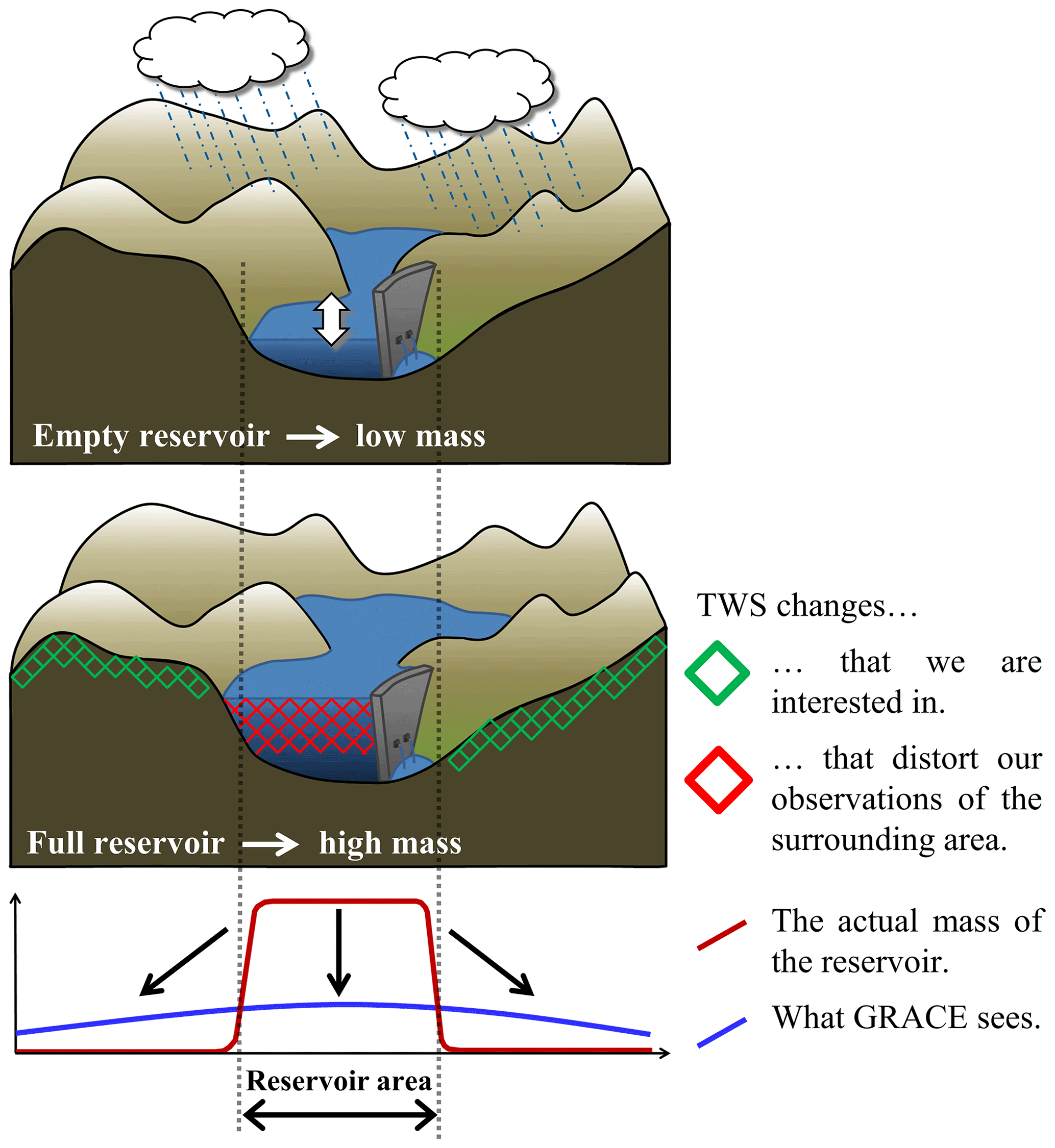
Figure 1Overview of the lake leakage problem with localized changes in water level of the lake/reservoir influencing the estimated water storage in surrounding areas.
This sub-scale mass variability impacts GRACE amplitudes up to 20 % averaged over basins as large as ∼ 200 000 km2 (Longuevergne et al., 2013; Farinotti et al., 2015). Although the issue of concentrated hydrological mass variations is not limited to surface waterbodies (e.g. Castellazzi et al., 2018), dam operations and impoundment have a large impact on the water cycle and on continent–ocean exchanges (Chao et al., 2008). Therefore, several publications have focused on removing the impact of surface waterbodies from GRACE total water storage changes. For example, Grippa et al. (2011) removed the influence of surface water storage in the Niger River (derived from altimetry and remotely sensed surface water extent) from GRACE TWS estimates to better be able to compare them to hydrological model output. Tseng et al. (2016) determined mass changes in two Tibetan lakes, combining altimetry, remote sensing, and GRACE estimates, and Zhang et al. (2017) estimated water volume changes for 96 % of the lake area on the Tibetan Plateau by combining an average of ICESat-derived elevation changes from a number of larger lakes with Landsat lake area changes for smaller lakes. Ni et al. (2017) removed the leakage error in GRACE estimates over Lake Volta in Ghana using constrained forward modelling. All these studies represent regional test cases, but a global assessment of the influence of surface waterbody mass change on GRACE data is missing.
Using GRACE data for the evaluation of (global) hydrological models or for combining models and observations by model calibration (Werth and Güntner 2010) and data assimilation (C/DA; Zaitchik et al., 2008; Eicker et al., 2014) without accounting for localized surface water storage can lead to two different kinds of errors. (i) Many global hydrological models do not include a surface water storage compartment at all (Scanlon et al., 2017), and assimilating GRACE TWS into a model that does not explicitly include surface waters will inevitably result in other storage compartments (such as soil moisture or groundwater) becoming distorted by absorbing the observed surface water mass change. Even if a model such as WaterGAP (Müller Schmied et al., 2014) does include a surface water compartment, it might not represent the realistic behaviour of, for example, human-operated reservoirs, and it might be preferable to exclude the reservoir storage from the assimilation. (ii) The leakage effect of localized surface waterbodies might cause an assimilation of the surface water mass change into neighbouring grid cells that should not be affected by it. To our knowledge, no investigation so far has studied the effects of surface waterbodies on GRACE model calibration or data assimilation and how they can best be handled in order to not distort the C/DA results. Having a global correction dataset to clear GRACE water mass changes of the influence of large surface waterbodies (here, lakes and reservoirs) will be immensely helpful for making GRACE estimates more consistent with model output.
Today, extensive information on surface water variations is available from satellite remote sensing. For almost 30 years, satellite altimetry has been providing water levels of large and medium lakes and reservoirs on a global scale (e.g. Birkett, 1995; Berry et al., 2005; Göttl el al., 2016). Several databases make these time series freely available for hydrological applications, among them the Database for Hydrological Time Series of Inland Waters (DAHITI; Schwatke et al., 2015). In addition, optical satellite images are used to derive surface extent of lakes and reservoirs (e.g. Pekel et al., 2016; Klein et al.,2017; Schwatke et al., 2019). Time series from optical sensors can reach a length of up to almost 40 years with a spatial resolution of 250 (MODIS, since 1999), 30 (Landsat, since 1982), and 10 m (Sentinel-2, since 2015) as well as a high temporal resolution with revisit time from 14 (Landsat), over 5 (Sentinel-2), and up to 1 d (MODIS). By combining height and surface area information, time series of storage changes can be derived purely based on remote sensing data (e.g. Schwatke et al., 2020; Busker et al., 2019; Crétaux et al., 2011).
To account for the second challenge in using GRACE data for hydrological studies, namely the removal of all non-hydrology-related mass variations, some effects are typically subtracted using geophysical models either during the computation of the gravity field solutions (e.g. Earth tides, ocean tides, and oceanic/atmospheric mass variations) or in post-processing (e.g. glacial isostatic adjustment (GIA)). However, in addition to this, the mass redistribution caused by the crustal deformation following large earthquakes is also contained in the GRACE observations masking hydrological phenomena in the affected regions. Several studies have highlighted GRACE's usefulness for estimating large earthquakes (Mw>9.0; e.g. Panet et al., 2007; Broerse, 2014; Einarsson et al., 2010; Einarsson, 2011; L. Wang et al., 2012) and have also identified co- and post-seismic earthquake signals in GRACE data with a lower magnitude (e.g. Han et al., 2016; Zhang et al., 2016), down to magnitude 8.3 (Chao and Liau, 2019). For example, the onset of the Sumatra–Andaman earthquake in December 2004 (magnitude 9.1) was analysed using, among others, differences of monthly gravity solutions (Han et al., 2006), wavelet analysis (Panet et al., 2007), Bayesian approaches (Einarsson et al., 2010), or normal modes (Cambiotti et al., 2011). At time of writing, the German GeoForschungsZentrum in Potsdam (GFZ) is the only processing centre that provides a total water storage (level 3) dataset corrected for earthquakes (Boergens et al., 2019); however, a data-based global earthquake correction for different GRACE solutions is not available yet.
To account for both the localized surface water storage in lakes/reservoirs and the earthquake signal, we present the first release of a new global correction dataset, RECOG (REgional COrrections for GRACE) RL01, which can be used for disaggregation of the integral GRACE water storage estimates in addition to applying standard corrections such as GIA models and the atmosphere/ocean de-aliasing products. The term RECOG refers to the fact that all effects included in the data product are localized phenomena that nevertheless influence a larger region around them. The surface water correction (RECOG-LR) was computed from forward-modelling altimetry and remote sensing observations and can be used (a) to subtract the lake/reservoir storage from the GRACE time series (removal approach) and (b) to relocate the surface water storage at its exact location of origin (relocation approach). The earthquake correction (RECOG-EQ) was estimated from GRACE monthly solutions using the Bayesian approach provided in Einarsson et al. (2010) and takes into account both the co-seismic and the post-seismic signal.
This paper is organized as follows: Sect. 2 describes the input data and processing steps, presents the resulting correction products, and visualizes some of its key characteristics. In Sect. 3 we then show different exemplary applications of the dataset in order to illustrate its impact and to demonstrate its value: influence of RECOG on GRACE time series including a short discussion of the impact on data assimilation into a global hydrological model, the detection of drought indices in an earthquake-affected region, and a validation of the correction product using GNSS-observed station displacements. This is followed by a discussion of the benefits and limitations of the correction product in Sect. 4, before Sect. 5 summarizes the findings and gives an outlook on further development options.
In this section we describe the various input data and their sources (Sect. 2.1.1 and 2.1.2) that were used to perform the forward modelling (Sect. 2.1.4) of the surface waterbodies and its necessary pre-processing steps (Sect. 2.1.3). The resulting lake/reservoir correction dataset, RECOG-LR, is discussed in Sect. 2.1.5. The processing steps for computing the earthquake correction are described in Sect. 2.2.1, followed by the results of RECOG-EQ (Sect. 2.2.2).
2.1 Lake/reservoir correction, RECOG-LR
The lake/reservoir correction is based on a subset of currently 283 of the largest surface waterbodies monitored with satellite altimetry (see Supplement S1 for a complete list). The lake water volume variations product is designed around (1) monthly water level time series from a global multi-satellite product and (2) the (static) surface water extent area for each lake.
2.1.1 Lake level time series from altimetry
Satellite altimetry measures the distance between the satellite and the Earth surface (i.e. the range) by analysing the transmitted and received radar echo after it has been reflected by the Earth's surface. Originally, the technique was developed for open-ocean applications. However, if the data are carefully pre-processed, they can also be used for estimating the height of inland waterbodies, such as lakes and reservoirs. Since the inland signals are frequently contaminated by land reflections, a rigorous outlier detection (Schwatke et al., 2015) as well as a dedicated retracking (e.g. Gommenginger et al., 2011; Passaro et al., 2018) is mandatory.
In this study, time series created by DAHITI (Schwatke et al., 2015) are used. DAHITI provides water level time series of more than 2000 globally distributed inland targets (i.e. lakes, rivers, and reservoirs) in a period between 1992 and today, depending on the satellite mission covering the waterbody. Data from altimeter missions TOPEX, Jason-1/-2/-3, ERS-2, Envisat, SARAL, Sentinel-3A/-3B, ICESat, and Cryosat-2 are combined in a Kalman filter approach after being retracked with the Improved Threshold retracker (Bao et al., 2009). A key element of the approach is an extended outlier detection before and after data combination, including an optional classification of the radar echoes. The temporal resolution of the time series differs depending on the size of a lake. Small lakes that are only covered by one single satellite track can be measured every 35 or 10 d (depending on the mission), whereas for large lakes a height can be derived almost every day. Moreover, information can only be provided for those waterbodies located directly beneath a satellite's tracks (Dettmering et al., 2020), preventing the creation of water level time series of small lakes located between the satellites' ground tracks. In addition, for small lakes or lakes surrounded by large topography no reliable height information might be created due to corrupted or too-noisy radar echoes.
The quality of the DAHITI water level time series depends on various criteria, mainly on the size of the lake and the length of the crossing satellite track as well as the surrounding topography. Comparison with in situ data show RMSE of a few centimetres for larger lakes and RMSE of some decimetres for river crossings (Schwatke et al., 2015).
2.1.2 Creating lake shapes from remote sensing
Based on MODIS optical satellite data, daily surface water extents are provided by the DLR's Global WaterPack (GWP) product (Klein et al., 2017). To receive reliable estimates of the extent of large global lakes and reservoirs, daily observations are aggregated to obtain maximum waterbody extents for the years 2003 to 2018. To capture coherent waterbodies, a pixel-based region-growing algorithm is applied, using ancillary information of the temporal static HydroLAKES dataset (Messager et al., 2016) for waterbody identification. Hereby, every water pixel in the aggregated GWP raster layer that spatially overlaps with the original HydroLAKES shape file is assigned to the lake ID given by the HydroLAKES database. Subsequently, a seed point in every designated waterbody is determined, from which 8-pixel growth of the search window region is initiated, thus identifying neighbouring water pixels. This ensures that waterbodies are represented by coherent pixel groups only. After the growing process is finished, results are vectorized. With this dynamic approach, the risk of over- or underestimation of the actual water surface extent is reduced (see Fig. S2 in the Supplement for further details).
2.1.3 Data pre-processing
The input data were combined taking into account several pre-processing steps: water level observations were averaged to a monthly mean for consistency with the temporal resolution of the GRACE gravity field models. Missing months were linearly interpolated. The water level time series were cut to the investigation period (January 2003–December 2016) and then reduced by their respective means. To ensure a quick update of the correction product when new lakes will be added to the source databases or when their time series will be updated, the algorithm for matching water level time series with their respective lake surface area (as well as most of the following workflow) was automated. The first step for the combination was an automatically generated data table with global common lake IDs. Where no IDs were available, matching was achieved by comparing names while making sure that no double naming occurred in the input data. If that was not possible or no names were given, matches were found using a very strict search algorithm for the nearest lake shape to a given time series. If none of the above methods was successful, the respective lake was dismissed and not included in the correction. In total, matches for 283 lakes/reservoirs were found for RECOG-LR RL01 (see Fig. 2); a detailed list is provided in the Supplement (Sect. S1). The surface waterbody shapes were then discretized on a fine-resolution, 0.025∘ grid to be able to capture long but narrow reservoirs in valleys. As in our algorithm grid cells are only assigned to belong to a waterbody if their midpoint lies within the lake polygon, small waterbodies would otherwise be missed completely. Multiplication with the altimetry-derived water height resulted in water volume estimates for each of the grid cells. These water volumes were subsequently distributed proportionally over a lower-resolution, 0.5∘ grid to save computation time in the forward modelling and because a 0.5∘ resolution is more than sufficient for applications to GRACE. The resulting global grids of lake/reservoir-related water height anomalies for each of the 168 months of our investigation period then entered the forward-modelling algorithm.
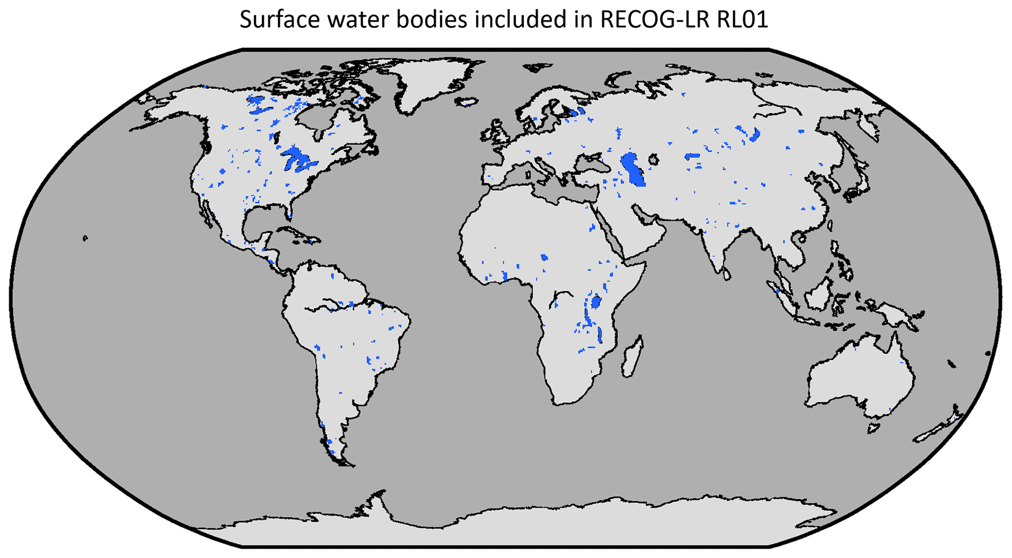
Figure 2Overview of all 283 lakes/reservoirs in the dataset (blue areas) given on a 0.5∘ grid.
2.1.4 Forward modelling
The localized altimetry/remote-sensing-derived surface water variations have to be converted to the GRACE spatial resolution before they can be subtracted from monthly GRACE gravity field estimates. In this forward-modelling step, the gridded values were expanded into spherical harmonic coefficients up to degree (n) and order (m) 96 according to
with ΔCnm and ΔSnm being the spherical harmonic coefficients (at degree n and order m), R the radius of the Earth, M the mass of the Earth, kn the load Love numbers (Farrell, 1972), ΔTWS(θλ) the changes in altimetry-derived water storage in relation to colatitude θ and longitude λ, and Pnm the Legendre functions. Subsequently a standard GRACE filter was applied for smoothing (DDK3; Kusche, 2007; Kusche et al., 2009). The filtered coefficients are then denoted by and . Differently filtered corrections are available upon request. This gives us the idealized signal that GRACE would measure if it were influenced by the changing mass in the lakes/reservoirs only. For a grid-based evaluation ( grid) a recomputation using Eq. (2) is necessary to calculate the lake water storage ΔTWSF(θ,λ) for every grid cell after filtering (Wahr et al., 1998), again up to degree and order 96:
Here we included the density of water ρ (1025 kg m−3) to obtain a lake water storage result in metres of equivalent water heights (EWHs), corresponding to the input variations in water storage from the water level time series.
2.1.5 Results for RECOG-LR
The resulting product for the lake and reservoir correction consists of two different parts, namely (1) the forward-modelled lake water correction to be subtracted from the GRACE data to remove the influence of lakes/reservoirs (removal approach). It is provided both on a spherical harmonic level (coefficients and ) and as a gridded data product (ΔTWSF(θ,λ) from Eq. 2). The second part consists of (2) the altimetry-derived monthly water levels for each 0.5∘ grid cell that can be used to re-add the measured lake volume to its actual area (relocation approach). Figure 2 highlights each grid cell that includes surface waterbodies with data used for the correction. Note that, although most of the major lakes and reservoirs are covered, some had to be excluded from the dataset for reasons explained further in Sect. 4. Figures showing an exemplary seasonal cycle of RECOG-LR can be found in the Supplement (Fig. S3), and an animation of the monthly changes of the lake/reservoir water storage for the full time series is provided in the “Video supplement” section (Deggim et al., 2020b; https://doi.org/10.5446/48188).
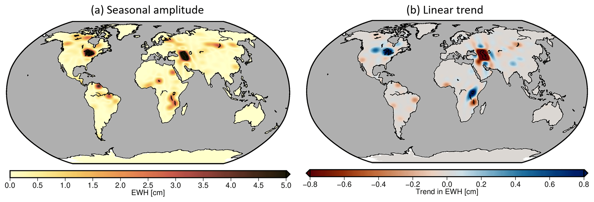
Figure 3RECOG-LR on a global scale with its (a) mean seasonal amplitude and (b) trend.
Figure 3a shows the mean amplitudes of the seasonal variations of the correction for each grid cell. The most prominent features are the Caspian Sea in Asia and the Great Lakes in North America with amplitudes of about 10 cm. However, peaks for individual months can reach as much as 30 cm of TWS correction, as shown for exemplary time series in Fig. S3. Most of the other lakes and reservoirs have mean correction amplitudes in the area of 0 to 3 cm. Figure 3b displays the linear trend of the lake correction product. Again, the most distinctive features are a strong negative trend of the Caspian Sea and a strong water storage increase in the Great Lakes (altimetry time series shown in Fig. S4 in the Supplement for comparison). Strongly visible is also a positive trend (mass increase) in Lake Victoria accompanied by a clear mass loss in the nearby Lake Malawi. However, it also becomes evident that some surface waterbodies can have a rather prominent trend signal without having a strong seasonality, as for example Lake Oahe in South Dakota, or exhibit a strong seasonality without any long-term trend, such as Lake Chad in Africa or Lake Guri and Tucurui Reservoir in South America. In other surface waterbodies, such as the artificial reservoir Lake Volta, the time series is dominated by a strong inter-annual signal (Ni et al., 2017), which does not show up prominently in Fig. 3 but is very much visible in the total temporal variability shown in Fig. 5 below.
2.2 Earthquake correction, RECOG-EQ
2.2.1 Processing of RECOG-EQ
Different from the lake/reservoir correction, which is computed by forward modelling using independent datasets (altimetry/remote sensing), the earthquake correction is derived by fitting a parametric function to monthly GRACE data along the following processing line: in a first step, spherical harmonic coefficients have to be backward-modelled to gridded geoid changes by
to be able to apply the Bayesian approach provided in Einarsson et al. (2010). The total geoid changes for a specific location (θi,λj) can be subdivided into a bias (ΔGCbias), trend (ΔGCtrend), annual- (ΔGCann) and semi-annual signal (ΔGCsemiann), S2 aliasing period of 161 d (ΔGCN2), and the earthquake signal (ΔGCEQ) as
which contains the model coefficients Cbias, Ctrend, Cann, ϕann, Csemiann, ϕsemiann, CS2, and ϕS2. The earthquake signal included here is described by a co-seismic and a post-seismic component modelled as
and describe coefficients for the co- and post-seismic component of the respective earthquake v, is the Heaviside step function at time tv, and τ is the decay rate. All coefficients are then estimated using Monte Carlo integration for quasi-linear models and are used to estimate the total earthquake signal. This signal is then removed from the total geoid changes for each considered earthquake to derive an earthquake-corrected dataset. Furthermore, we applied a spatial radial Gaussian window with a radius (half width) of 157 km to consider only regions that were affected by earthquakes. The centre of the Gaussian window is placed in the epicentre of the respective earthquake. Einarsson's approach is, as recommended, consecutively applied to earthquakes with a magnitude that is larger than or equal to 9.0, which is a criterion met by the Sumatra–Andaman earthquake (M9.1) in December 2004 and the Tohoku earthquake (M9) in March 2011. Einarsson (2011), for example, showed that earthquakes with a magnitude larger than 9.0 are clearly visible in GRACE data, while earthquakes with lower magnitude cannot always be clearly separated. For more information about the approach see Einarsson et al. (2010) and Einarsson (2011). To derive TWS anomalies, the geoid changes are forward-modelled to spherical harmonic coefficients similar to Eq. (1) by
and again backward-modelled to TWS changes as described in Eq. (2). The final earthquake correction product, RECOG-EQ, is then derived by computing the difference between the uncorrected and earthquake-corrected TWS anomalies (TWSA).
2.2.2 Results for RECOG-EQ
The correction is provided equivalently to the lake correction: the dataset is processed on a global 0.5∘ grid using spherical harmonic coefficients up to degree and order 96, is DDK3-filtered (different filters are available upon request), and covers the period 2003 to 2016.
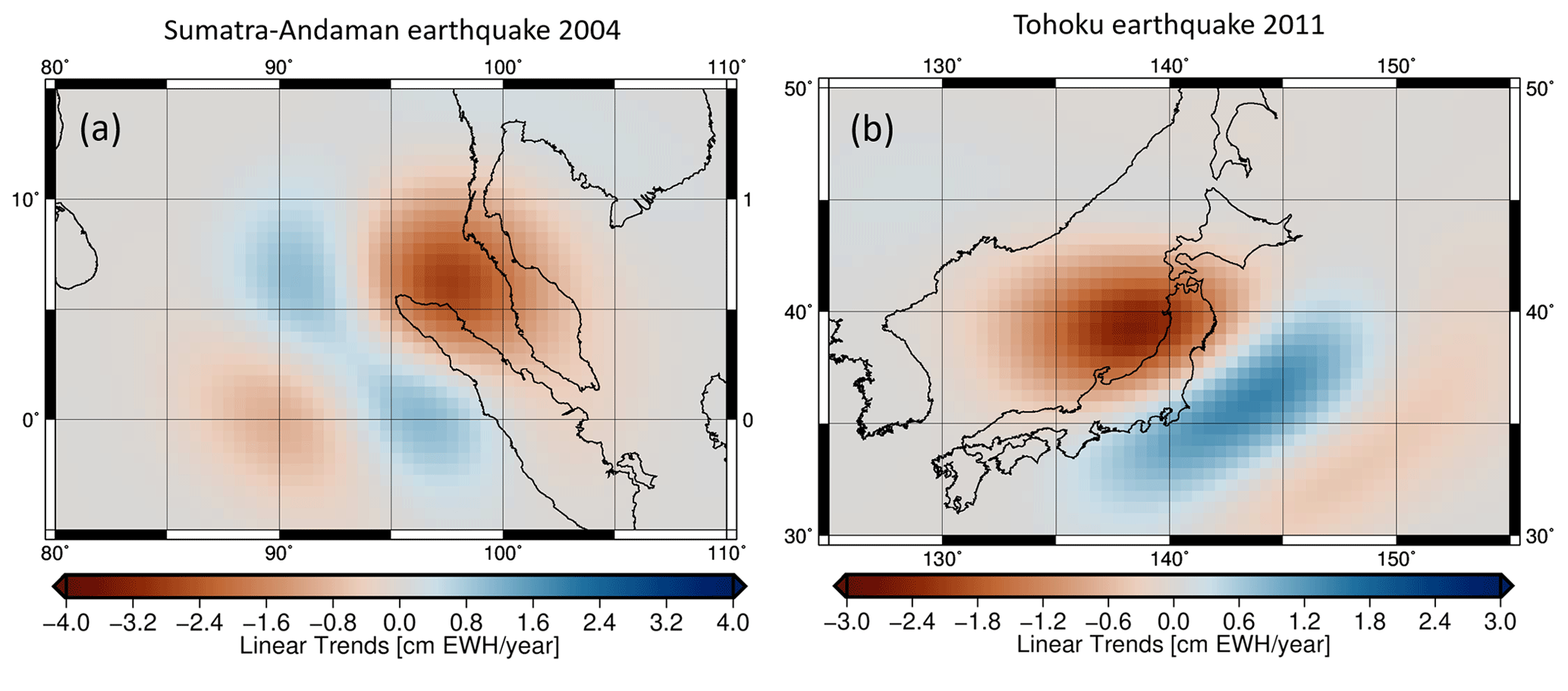
Figure 4Linear trends (January 2003–December 2016) of TWS changes (cm EWH yr−1) of the earthquake correction that includes the (a) Sumatra–Andaman earthquake from 2004 and the (b) Tohoku earthquake from 2011.
The correction only shows differences over the regions of the 2004 Sumatra–Andaman earthquake (Fig. 4a) and the 2011 Tohoku earthquake (Fig. 4b) because we only corrected for these two earthquakes. For the Sumatra–Andaman region the linear trends of the correction reach from about −2.7 to 1.1 cm EWH per year. Negative linear trends of down to −2.7 cm EWH per year can be found north of Indonesia and west of peninsular Malaysia, while positive trends are visible in the Indian Ocean close the coast of Sumatra. Considering Tohoku, the linear trends range from about −2.5 to 1.4. The dominant negative part can be found to the west of the Tohoku region, while the positive parts are apparent in the Pacific Ocean, southeast of Tohoku. These results suggest that uncorrected TWS changes might hinder the correct analysis of the data for hydrological studies, because the post-seismic part of the earthquake might falsely be interpreted as a linear trend in the uncorrected TWS changes. This is particularly relevant when the earthquake occurs at the beginning of the time series as is the case for the Sumatra–Andaman earthquake. The results shown here are derived from the ITSG-Grace2018 solutions (Kvas et al., 2019). Earthquake corrections derived from other GRACE solutions provide similar findings; for completeness they are attached in the Supplement (Figs. S5 and S6). We do not apply geophysical forward modelling since these models heavily depend on dislocation parameters, fault geometry, and background rheology, and parameters are typically tuned to fit seismic and GNSS measurements but do not fit observed gravity changes.
In this section we would like to show the influence and benefit of the correction datasets. For this purpose, in Sect. 3.1 we first illustrate the impact of subtracting the two corrections RECOG-LR and RECOG-EQ from the GRACE time series in terms of change in signal variability and trends. This includes a short discussion of the benefit of RECOG-LR for data assimilation into hydrological models, one of the main target applications of the corrected GRACE dataset. The comparison to GNSS surface displacements (Sect. 3.2) not only shows the influence of the surface water correction on geometrical surface deformations even several hundreds of kilometres around lakes/reservoirs but also represents a first validation of the corrected GRACE time series using independent observations. Finally, the influence of removing earthquake signals (RECOG-EQ) for hydrological drought detection is described in Sect. 3.3.
3.1 Influence of RECOG RL01 on a global GRACE time series
3.1.1 Influence of lake/reservoir correction, RECOG-LR, on GRACE
We first investigate the influence of subtracting the lake/reservoir correction dataset from a global GRACE time series. For this purpose, we derive gridded TWSA from the ITSG-Grace2018 (Mayer-Gürr et al., 2018; Kvas et al., 2019) spherical harmonic expansion up to degree and order 96 considering corrections for low-degree coefficients (Swenson et al., 2008; Cheng et al., 2011; Sun et al., 2016), glacial isostatic adjustment (A et al., 2013), and applying the DDK3 filter (Kusche, 2007).
For the removal approach, we then reduce the lake correction (Sect. 2.1.5) from the GRACE-derived TWSA grids. For the relocation approach, we re-add the altimetry-derived monthly water mass estimates. This leads to three global TWSA datasets: (1) GRACE-based only, (2) GRACE TWSA after removing altimetry-based lake/reservoir storage, and (3) GRACE TWS with relocated altimetry-based lake signal.

Figure 5Temporal root mean square (rms) of the lake/reservoir correction time series for each grid cell (a) and the relative reduction in temporal rms when subtracting the correction (removal) from the original GRACE TWS time series (b).
Figure 5a shows the temporal root means square (rms) of the lake correction for each grid cell. Subtracting this correction reduces the temporal rms variability in the GRACE time series (Fig. 5b) by up to 75 % around the Caspian Sea in Asia and 50 % around Lake Victoria in Africa, compared to the original variability in ITSG-Grace2018. Values around the other lakes vary between 0 and 30 % with a few negative values in the area south of the Caspian Sea and in Canada. The latter can most likely be attributed to Gibbs oscillations by the bandlimited spectral representation of the data and/or to being spuriously introduced by the non-isotropic DDK3 filter applied to the lake signals. However, the option that the lake signal was hiding another impact, which can only be recovered after subtracting the correction, should not be completely ruled out, e.g. in the case of water transfer between compartments as from glacier/snow to lake water (Castellazzi et al., 2019).

Figure 6Linear trend of GRACE TWS anomalies (January 2003–December 2016) in the Caspian Sea region (a–c) and in the Mississippi Basin and around the Great Lakes (d–f) without any correction (a, d), after removing the influence of lakes (b, e), and after relocating the lake signal (c, f). Please note that the Aral Sea has been excluded from RECOG-LR RL01 due to its strongly varying surface area, which is not yet captured in the database.
Figure 6 shows the influence of the lake correction on the linear trend in the GRACE time series for two detailed examples; a global map can additionally be found in the Supplement (Fig. S7). In the area around the Caspian Sea (Fig. 6a–c), a very strong negative trend of around −3 cm yr−1 in the original GRACE time series (a) is almost completely removed by the lake correction (b). The relocation approach then restores the altimetry-derived lake water variation to the lake area (c). The second example shows the Mississippi Basin (Fig. 6d–f). Even though the Great Lakes are not part of the basin, they still have an effect, particularly on subbasin Alton (upstream from Alton, Illinois, USA), which is closest to the Great Lakes. Influences of the lake variations on the GRACE basin average of this subbasin can reach values of up to 5 cm in TWS for some months. This example also shows that a positive trend visible in the original GRACE data can mainly be attributed to surface water change and can be levelled by the correction. Subtracting the lake correction also reduces the positive trend partly caused by smaller lakes/reservoirs (e.g. Lake Oahe and Lake Sakakawea) in the Hermann subbasin in the northwest of the Mississippi.
The importance of correcting the signal in the nearby Great Lakes and the smaller lakes/reservoirs within the subbasins can also be detected when assimilating GRACE-derived TWSA into a hydrological model. The original and the RECOG-corrected, subbasin-averaged GRACE TWSA of the Mississippi River basin were assimilated into the Water – Global Assessment and Prognosis (WaterGAP; Döll et al., 1999; Alcamo et al., 2003; Müller Schmied et al., 2014) hydrological model, which has a grid spatial resolution. Our assimilation theory follows Eicker et al. (2014) and Schumacher et al. (2015, 2016); for more information see the Supplement (Sect. S8).
In the Alton subbasin, the assimilation of the original GRACE observations introduces a spurious positive mass trend of 2.5 mm EWH yr−1 not present in the original WaterGAP version. This trend is assumed to not originate from storage increase within the subbasin itself but to be caused by leakage due to a water storage increase in the Great Lakes (see Fig. 6), particularly in the nearby Lake Superior and Lake Michigan. Applying the RECOG correction dataset before assimilation reduces the linear trend in the subbasin to 0.9 mm EWH yr−1 and thus prevents the spurious trend from appearing in the model output. This can also be confirmed on the grid cell level with a trend reduction in 53 % of the grid cells in the Alton subbasin, 40 % of them by more than 80 % compared with the results of assimilating the original TWSA. The strongest reductions appear in the northeastern part of the basin, e.g. from 12.3 to 3.5 mm EWH yr−1 in a grid cell in close proximity to the Great Lakes (lat 46.25∘, long −90.25∘). In grid cells directly affected by lake water storage the effect can be even larger; e.g. for Lake Sakakawea (lat 48.25∘, long ) the trend in the assimilation results changes from 493.5 to 8 mm EWH yr−1, and the signal rms from 2548 to 120 mm. The results reveal the importance of applying a lake water correction to GRACE data before data assimilation not only for areas covered by waterbodies but also for neighbouring grid cells affected by strong leakage-in effects.
3.1.2 Influence of earthquake correction, RECOG-EQ, on GRACE
This section presents the application of the earthquake correction (Sect. 2.2) to the GRACE data. Linear trends for the period 2003 to 2016 are derived from (1) the original GRACE TWSA and (2) the corrected TWSA after applying RECOG-EQ. The correction changes the spatial pattern of the linear trend in the Sumatra–Andaman region (Fig. 7a and c), and the magnitude of positive trends increases by about 0.5 cm EWH yr−1 from 4.2 to 4.7 cm EWH yr−1. The spatial extension of the positive trends in the corrected data (Fig. 7c) reaches to peninsular Malaysia. Thus, the former slightly negative trends of about −1 cm EWH yr−1 identify a smaller magnitude or even slightly positive values in the earthquake-corrected dataset. The change in trends might bias the correct analysis of linear trends for this region.
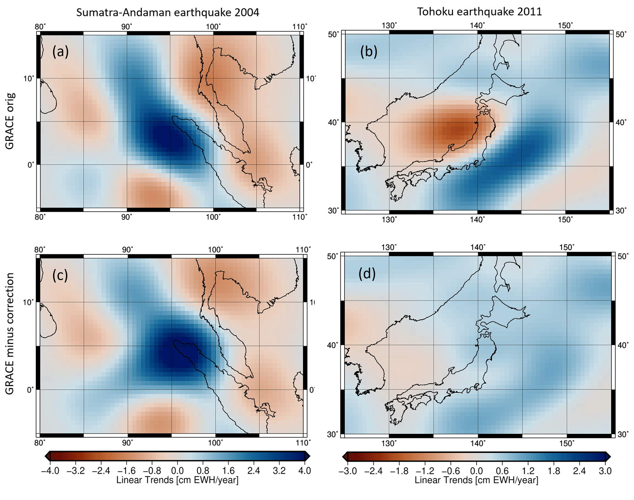
Figure 7Linear trends (January 2003–December 2016) of TWS changes (cm EWH yr−1) before and after removing earthquake signals of the Sumatra–Andaman earthquake from 2004 (a, before; c, after) and the Tohoku earthquake from 2011 (b, before; d, after).
When analysing the Tohoku earthquake results (Fig. 7b and 7d), we also see that the magnitude and spatial pattern of the trends change. In this case, the difference between original and corrected GRACE data is more obvious than in the Sumatra–Andaman region: the original dataset shows positive linear trends of about 2 cm EWH yr−1 in the west of Tohoku, while negative trends of about −2 cm EWH yr−1 can be found in the Pacific Ocean along the southeastern coast. These trend signals vanish almost completely after subtracting the earthquake correction, confirming our assumption made in Sect. 2.2.2: the post-seismic earthquake component was identified as linear trends in the original GRACE data and has clearly biased the trend analysis, leading to misinterpretation of the trends, especially for the Tohoku region.
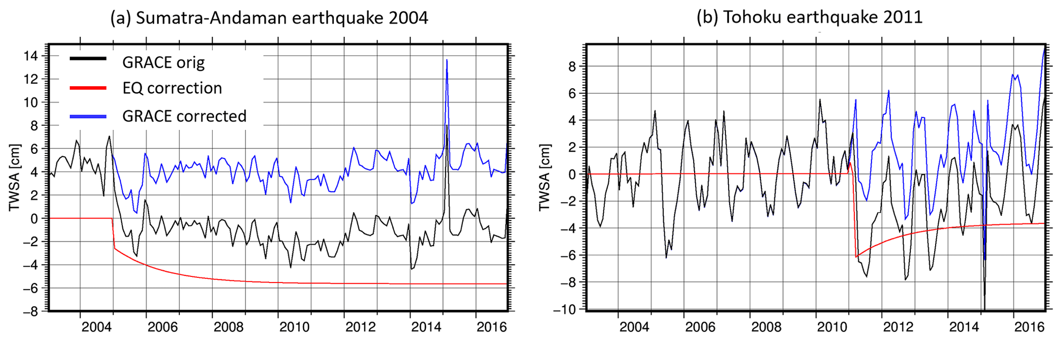
Figure 8Spatially averaged GRACE TWS anomalies for the original (black) and earthquake-corrected (blue) GRACE data and its correction (red) for (a) peninsular Malaysia (West Malaysia) and (b) Japan.
To analyse the effect of earthquakes on TWS changes in more detail and over land, spatially averaged TWS anomalies are compared for peninsular Malaysia in Fig. 8a and for Japan in Fig. 8b. Additional figures showing the signal in the epicentre of the two earthquakes are shown in the Supplement (Fig. S9). Regarding peninsular Malaysia, the uncorrected TWSA (black) show a strong decrease in TWS changes beginning in 2004, which results from the Sumatra–Andaman earthquake. After applying the correction (blue), this strong decrease is removed. The correction (red) shows nicely the co-seismic component of about −2.5 cm EWH as a jump between December 2004 and January 2005 and a following post-seismic relaxation, which increases the total correction towards −6 cm. Similar findings can be observed for the results for Japan and the Tohoku earthquake: the correction contains a co-seismic component down to −6 cm with post-seismic relaxation afterwards, but in this case the relaxation is slowly decreasing the amount of correction. However, both examples clarify that uncorrected GRACE data could lead to wrong conclusions about the underlying signals as the apparent trends can, for instance, hamper the identification of drier and wetter years in the GRACE time series.
3.2 Validation of RECOG-LR with GNSS
Global Navigation Satellite System time series contain signals resulting from surface mass redistribution: atmospheric pressure, non-tidal oceanic loading, and hydrological changes. Vertical displacement due to hydrological loading can be predicted by calculating the elastic response of an Earth model to the TWS changes. Previous studies have shown good agreement between modelled deformation from GRACE TWS and vertical displacement observed by GNSS (e.g. Springer et al., 2019; Tregoning et al., 2009; van Dam et al., 2007), while horizontal displacements due to hydrological loadings are much smaller than the vertical ones and have been found to be systematically underpredicted and out of phase (Chanard et al., 2018).
Here we use vertical displacement residuals from the ITRF2014 stacking (Altamimi et al., 2016) resulting from the second reprocessing campaign (repro2) by the International GNSS Service (IGS) (Rebischung et al., 2016) to validate the GRACE lake/reservoir correction data product RECOG-LR. The station velocities and discontinuities have been carefully removed from the GNSS time series. To be consistent with GRACE TWS, the effects of atmospheric and non-tidal oceanic loading are subtracted from the time series using the AOD1B product (Dobslaw et al., 2017). The displacements due to non-tidal oceanic and atmospheric loading are calculated at daily epochs to be consistent with the GNSS observations. GRACE TWS anomalies are converted into displacements in the spatial domain using spatial convolution of a point mass load Green's function (Farrell, 1972) in the centre-of-figure frame using a set of high-degree load Love numbers determined by H. Wang et al. (2012) for the Preliminary Reference Earth Model (PREM) (Dziewonski and Anderson, 1981). Finally, the daily GNSS displacements are averaged to monthly intervals before removing the temporal mean and linear trend from both GNSS-observed and GRACE-derived (modelled) displacements. Exemplary time series for GNSS-observed and GRACE-modelled displacements at different stations in the Great Lakes, Lake Victoria, and Caspian Sea regions are shown in the Supplement (Fig. S10). Here the GNSS time series are used to assess the impact of the lake/reservoir correction on GRACE data. To get an idea of the magnitude of its influence, we first show the temporal rms of the forward-modelled RECOG-LR signal (Fig. 9a) for ITRF2014 GNSS sites around the Great Lakes. This represents the signal variability of modelled station displacements caused only by the surface water variations described in RECOG-LR. The rms of the vertical displacements amounts to up to 1.4 mm for station ALGO (∼190 km away from the lake shore) and can reach higher values for other stations provided by NGL (Blewitt et al., 2018) (not shown), such as 2.3 mm at station BAKU close to the Caspian Sea and 2.5 mm at CHB5 directly at the shore of Lake Huron.
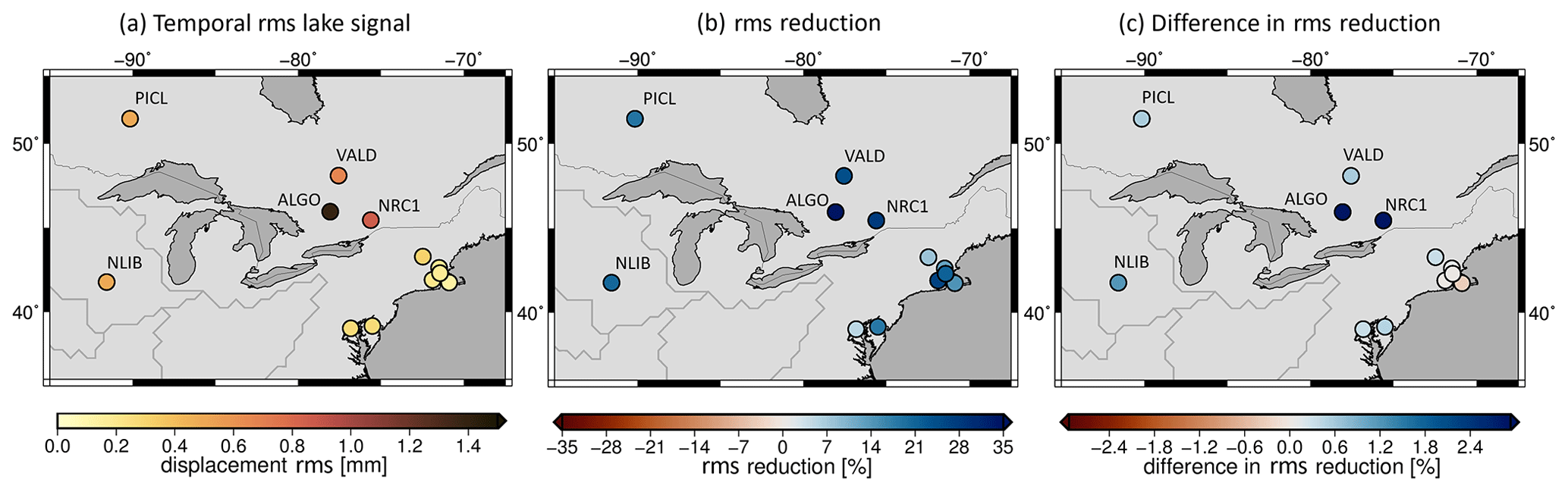
Figure 9Temporal rms of the vertical displacement caused by the forward-modelled lake/reservoir signal of RECOG-LR (a), reduction of rms of GNSS time series after subtracting modelled deformation (b), and difference in rms reduction when subtracting GRACE after removing and relocating RECOG-LR vs. using the uncorrected GRACE signal (c).
To investigate the agreement of observed (GNSS) and GRACE-derived displacement time series, we compute the reduction in temporal rms after subtracting the modelled displacements from the observed time series. For this we first compute the signal variability rmsGNSS of the observed station displacements and subsequently the variability rmsGNSS-GRACE of the GNSS time series after subtracting GRACE-derived station movements. The relative reduction in the rms is given by the following equation:
This relative reduction in rms is shown in Fig. 9b, and it can be observed that, by removing the modelled displacement based on GRACE from the GNSS time series, all stations around the Great Lakes have their rms reduced, indicated by positive rms reductions. This means for ITRF2014 GNSS sites around the Great Lakes we can explain some of the observed vertical displacement by TWS changes at most of the stations, with a stronger agreement at stations closer to the Great Lakes (ALGO and NRC1 stations).
To assess the influence of RECOG-LR on these reductions, we compute two different versions of Eq. (7): we compare the rms reductions using (1) the original (unmodified) GRACE data and (2) GRACE after subtracting and relocating the lake signal. The difference between these two rms reductions is plotted in Fig. 9c. A positive value means that the RECOG-corrected GRACE signal explains a better portion of the observed GNSS station displacements than the uncorrected GRACE signal. All but one of the stations around the Great Lakes show a positive effect of the lake correction. The only station unimproved is located quite far from the lakes, directly at the coast of the ocean, and might primarily be influenced by oceanic leakage as discussed in van Dam, et al. (2007). The largest improvements can be observed at stations ALGO (6.1 %) and NRC1 (4.3 %), both around 180–200 km away from Lake Huron. In the time series plot in Fig. S10 of the Supplement this improvement is indicated by a better fit of the corrected GRACE time series with the GNSS observations. Also for other ITRF2014 stations in the area of large surface waterbodies we find a systematic improvement of the rms reduction when applying RECOG-LR. Examples are stations around the Caspian Sea (NSSP: 0.2 % improvement; TEHN: 0.3 % improvement) and around Lake Victoria (NURK: 1.4 % improvement; RCMN: 2.7 % improvement). Here it should be noted that these stations are not located close to the shore but between 100–400 km away from the lakes, yet they are still affected by the correction of the lake signal. To put these numbers of up to 6 % improvement into perspective, a change in the Earth model used for the conversion of TWS to deformation, which has previously been found to be relevant for GNSS analysis (Karegar et al., 2017), has a much smaller influence. The differences in rms reduction using, for example, different sets of load Love numbers amount to only <0.4 %. Thus, from the above results, we are confident that correcting for the leakage effect of lake/reservoir water storage in GRACE time series can have a considerable positive effect on the comparison of GRACE and GNSS observations.
3.3 Hydrological drought detection with earthquake correction, RECOG-EQ
Hydrological drought detection using GRACE data has been applied in various studies, for example in Houborg et al. (2012), Thomas et al. (2014), Zhao et al. (2017), Boergens et al. (2020), and Gerdener et al. (2020a) for many regions of the Earth. Removing the earthquake signal before the analysis might lead to a change in the drought detection results, which could have a significant impact on, for example, the decisions of policy makers. In this section, we show an example of the influence of the earthquake correction (Sect. 2.2) for detecting drought events in peninsular Malaysia. To show the longer-term behaviour of droughts, the drought severity index using accumulation (DSIA) used in Gerdener et al. (2020a) is computed. As typically done with meteorological indicators, the observable is accumulated for a chosen period q () before its computation because we refer it to a duration of drought. For example, if the accumulation period q is set to 3 months, the accumulated TWS changes for March 2003 will be the sum of TWS changes of January, February, and March. The accumulation also serves as a running mean. The DSIA is then computed by
where is the accumulated TWS changes in year i and month ; is the mean monthly accumulated TWS change, e.g. the mean over all Januaries; and is the monthly standard deviation. Here, it is used to identify hydrological drought events for an accumulation period of 6 months (DSIA6) over peninsular Malaysia. Figure 10 shows the resulting DSIA6 time series using corrected (blue) and uncorrected (black) TWS changes. The uncorrected DSIA6 identifies a mainly moderate dry period in 2010 and 2011 and a severe period at the beginning of 2014. Both periods are also identified using the corrected DSIA6 but with different intensity. The period 2010/11 is slightly more intense now, and the drought in 2014 is extreme (e.g. Tan et al., 2017). Furthermore, the corrected DSIA6 shows exceptional drought in 2005, which was not identified with the uncorrected DSIA6. These findings are supported by, for example, the EM-DAT database (EM-DAT, 2020) and Hashim et al. (2016), who also identified a drought over peninsular Malaysia in 2005. However, in March 2005, a second earthquake (Nias earthquake) also occurred close to the Sumatra–Andaman region with a magnitude of M8.6. As stated by, for example, Broerse (2014), earthquakes with a lower magnitude are not always clearly visible in the data, but it should be noticed that the Nias earthquake might still have possible influences on the time series analysis.
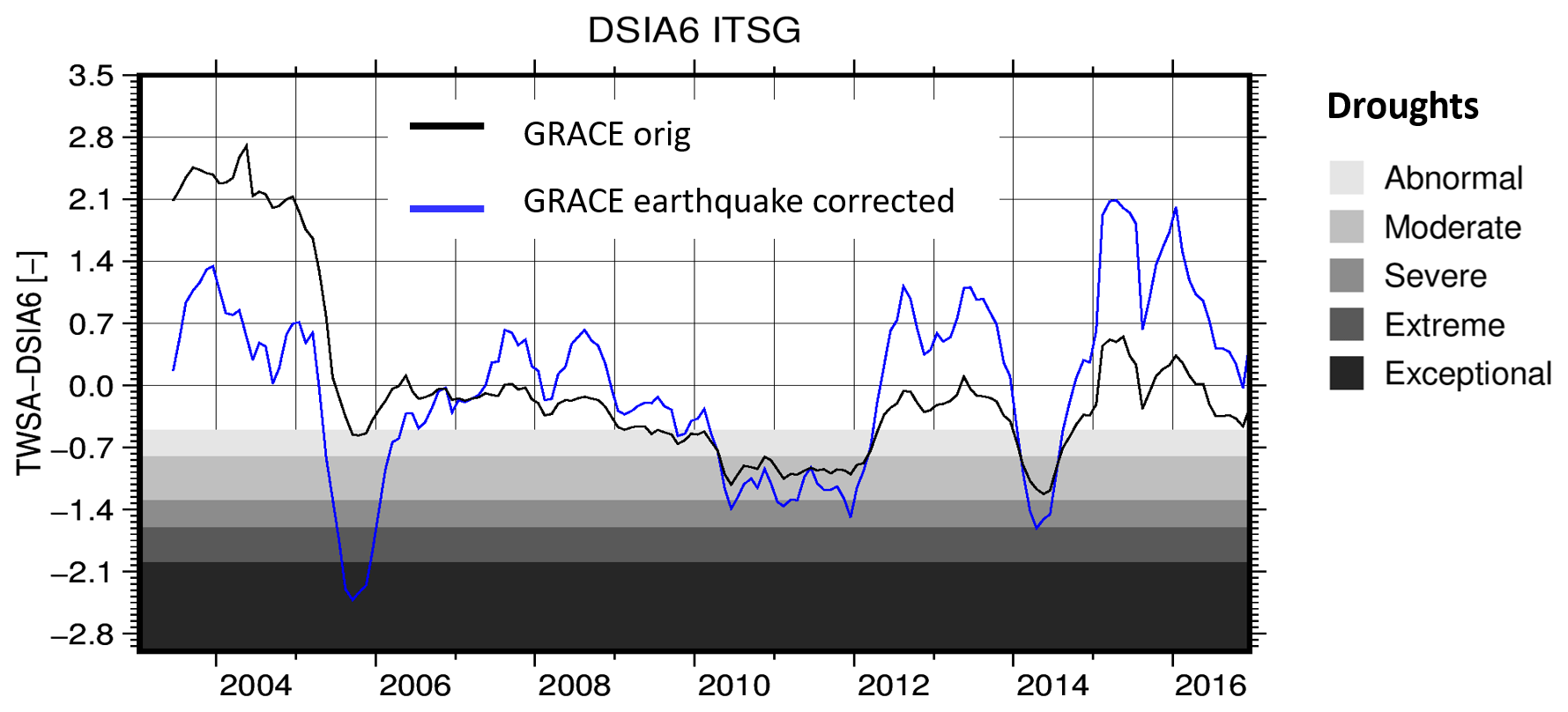
Figure 10GRACE-derived TWSA DSIA6 over peninsular Malaysia (West Malaysia) shown without (black) and with (blue) earthquake correction.
As mentioned in Sect. 2.1, static lake shapes were used to determine the lake volume and subsequently the mass estimates in this first release of RECOG. In contrast to monthly or daily lake shapes, these are not (or much less) impacted by cloud coverage in the optical satellite images and, thus, more reliable. This approximation works for most of the lakes with shores that are not too flat. Estimated errors caused by ignoring the changing surface area revealed numbers between 3–15 % for exemplary surface waterbodies (Semmelroth, 2019). Extreme cases with either very flat shores and high water level variations or strong trends such as the Aral Sea in Asia, whose surface area shrunk to a fraction of its original size in the last couple of decades, have been omitted in the correction.
Though RECOG-LR covers most of the major lakes around the world, some are not yet implemented in the dataset due to failed automatic matching between water level time series and lake surface area (e.g. Lake Athabasca, see also Sect. 2.1.3), insufficient water level time series due to ice coverage for major parts of the year (e.g. Lake Taymyr) or missing flyovers by altimeter satellites (e.g. Dead Sea; see also Sect. 2.1.1). More generally, we only consider surface waterbodies that can be captured by satellite altimetry and this way underestimate the impact of surface water storage in regions with a large number of small lakes and dams, e.g. in the US or in India.
Additionally, changes in surface water volume also affect surrounding groundwater storage (and thus GRACE data) by groundwater–surface water interactions (e.g. Bierkens and Wada 2019), which have not yet been considered in our data product. Steric effects caused by the thermal expansion of water have an influence on the altimetry-derived water levels in large surface waterbodies, which have not been accounted for in the conversion from water volume to mass change. Studies only exist for very large lakes, such as the Caspian Sea, where the steric water level change was found to amount to about of the seasonal amplitude (Chen et al., 2017; Loomis and Luthcke, 2017). We expect this to be an extreme case, with the influence on smaller waterbodies being considerably smaller. However, since the necessary temperature and salinity profiles are not available on a global scale including smaller waterbodies, no steric correction has been included in RECOG-LR.
The GROOPS software toolkit has been used. It is available on GitHub: https://github.com/groops-devs/groops/commit/a52631fc1817acdc4b40e1caae546254f36a2653 (last access: 6 November 2020; Mayer-Gürr et al., 2020).
RECOG includes (1) RECOG-LR with (1a) global gridded time series for the given time span with the correction values in total water storage for each grid cell and month, (1b) the same values in SH coefficients of degree and order 96, and (1c) the monthly gridded altimetry-derived water height for the relocation approach and (2) RECOG-EQ with the monthly gridded earthquake correction for TWS changes, containing the 2004 Sumatra–Andaman and the 2011 Tohoku earthquake. The data have been uploaded to the PANGAEA database: RECOG-LR: Deggim et al. (2020a), https://doi.org/10.1594/PANGAEA.921851; RECOG-EQ: Gerdener et al. (2020b), https://doi.org/10.1594/PANGAEA.921923.
Leakage effects of surface waterbodies and non-hydrology-related mass change signals have a strong influence on water storage estimates from GRACE, complicating its use for hydrological studies and specifically for calibration and data assimilation. Volume change estimates from combining satellite altimetry with remote sensing information can be used to remove (or at least strongly reduce) the effect of lakes and reservoirs from the GRACE data on a global scale, with particular benefit in regions close to big lakes/reservoirs or in regions with many smaller lakes and reservoirs. The earthquake signal (co-seismic and post-seismic), which masks hydrological variations in the vicinity of large earthquakes, can be extracted directly from the GRACE time series.
In this contribution, we introduced the first release of a new global correction dataset, RECOG RL01, for removing both the lake/reservoir storage (RECOG-LR) and the earthquake signal (RECOG-EQ) from the GRACE time series, while also offering the possibility to relocate the altimetry-derived mass change to its original surface waterbody outline.
Exemplary applications show that the correction product can reduce the signal variability (rms) of the GRACE signal by up to 75 % for the most prominent example of the Caspian Sea and that affected areas not only include the lake areas themselves but can also extend for tens to hundreds of kilometres around the waterbodies due to leakage. Special precaution has to be taken when assimilating GRACE data into hydrological models in the proximity of large surface waterbodies. In this context, the correction product is particularly valuable for models that do not include a surface water compartment at all, but the reduction of the leakage effect can also make it beneficial for models that do. For the example of the Alton subbasin of the Mississippi the leakage signal of the Great Lakes would cause an artificial mass increase in the assimilated model runs of WaterGAP, which can be prevented by subtracting and relocating the surface water storage before assimilation. A validation of the corrected GRACE signal using observed vertical GNSS station displacements shows an improvement of the fit between GRACE and GNSS of up to 6 % for stations at around 180–200 km distance from the Great Lakes. Applying the earthquake correction allows for the determination of several severe and one exceptionally severe drought events in peninsular Malaysia, which a GRACE-based drought indicator would otherwise have missed without first correcting for the earthquake signal. Therefore, depending on the application at hand, we recommend applying both RECOG-LR (globally) and RECOG-EQ (especially when research is performed in areas that underlie large earthquakes) as a standard post-processing step for analysing GRACE data.
Future improvements of the correction data product will introduce dynamic lake shapes replacing the static lake surface areas used so far, which will enable the inclusion of surface waterbodies with major area changes, such as the Aral Sea. Alternatively, pre-processed volume change time series of DAHITI (Schwatke et al., 2020) can be introduced for lakes for which they are already provided. The GRACE time series continues thanks to GRACE-Follow-On, and it is thus important to also provide a continuously updated surface waterbody correction which will rely on continuously updated source data. An extension of the RECOG-LR to include further surface waterbodies and a closure of existing data gaps as soon as new data are added to DAHITI will easily be possible thanks to a largely automated process of matching lake IDs in the altimetry database with corresponding lake shapes and forward-modelling the water volume to filtered GRACE-like TWS. Thus RECOG-LR can be updated as soon as new data become available.
So far, RECOG-LR focusses on lakes and reservoirs. However, there are other forms of surface waterbodies whose effects on GRACE data are still disregarded and not yet covered by any correction. An example for this are rivers, especially river deltas of big river basins (e.g. Mississippi, Amazon, Congo) that are highly influenced by strong seasonal variations in water flux as well as influences by tides in the estuary. Such a correction would be especially interesting for hydrological modelling.
The correction data product can also be extended to cover additional geophysical phenomena. For example, since most hydrological models do not include an explicit glacier compartment, it would be beneficial to extend the correction dataset to remove the glacier mass component from an independent glacier model or from remote sensing information before assimilating GRACE data into the model.
The presented correction products offer possibilities for more sophisticated data assimilation strategies. For example, GRACE data after removal of the lake/reservoir/earthquake correction can be assimilated into non-surface water compartments of a hydrological model, while the altimetry-derived relocation dataset can be assimilated solely into the surface water compartment of models that explicitly incorporate this. The best way to use this information for data assimilation will have to be further investigated.
Further research for the earthquake correction should consider comparing different methods and should also analyse possible influences of earthquakes with a magnitude lower than 9.0 in more detail.
A time-lapse video of RECOG-LR showing global correction maps for each month has been uploaded to the AV-Portal of the TIB Hannover: Deggim et al. (2020b), https://doi.org/10.5446/48188.
The supplement related to this article is available online at: https://doi.org/10.5194/essd-13-2227-2021-supplement.
RECOG-LR was created by SD, based on ideas and suggestions from AE and LL and with help from LS. RECOG-EQ was created by HG and JK. SM and IK (Sect. 2.1.1) and LE, CS, and DD (Sect. 2.1.2) provided input data. KS, OE, and JK performed the data assimilation, and ATS and TvD the validation with GPS. LS, AE, and SD created the figures. All authors contributed to and reviewed the manuscript.
The authors declare that they have no conflict of interest.
This research has been supported by the Deutsche Forschungsgemeinschaft and the Luxembourg National Research Fund within the framework of the Research Unit GlobalCDA (grant no. FOR2630).
This paper was edited by Christian Voigt and reviewed by Ki-Weon Seo and one anonymous referee.
A, G., Wahr, J., and Zhong, S.: Computations of the viscoelastic response of a 3-D compressible Earth to surface loading: an application to Glacial Isostatic Adjustment in Antarctica and Canada, Geophys. J. Int., 192, 557–572, https://doi.org/10.1093/gji/ggs030, 2013.
Alcamo, J., Döll, P., Henrichs, T., Kaspar, F., Lehner, B., Rösch, T., and Siebert, S.: Development and testing of the WaterGAP 2 global model of water use and availability, Hydrolog. Sci. J., 48, 317–337, https://doi.org/10.1623/hysj.48.3.317.45290, 2003.
Altamimi, Z., Rebischung, P., Métivier, L., and Collilieux, X.: ITRF2014: A new release of the International Terrestrial Reference Frame modeling nonlinear station motions, J. Geophys. Res.-Sol. Ea., 121, 6109–6131, https://doi.org/10.1002/2016JB013098, 2016.
Bao, L., Lu, Y., and Wang, Y.: Improved retracking algorithm for oceanic altimeter waveforms, Prog. Nat. Sci., 19, 195–203, https://doi.org/10.1016/j.pnsc.2008.06.017, 2009.
Berry, P. A. M., Garlick, J. D., Freeman, J. A., and Mathers, E. L.: Global inland water monitoring from multi-mission altimetry, Geophys. Res. Lett., 32, l16401, https://doi.org/10.1029/2005GL022814, 2005.
Bierkens, M. F. and Wada, Y.: Non-renewable groundwater use and groundwater depletion: a review, Environ. Res. Lett., 14, 063002, https://doi.org/10.1088/1748-9326/ab1a5f, 2019.
Birkett, C. M.: The contribution of TOPEX/POSEIDON to the global monitoring of climatically sensitive lakes, J. Geophys. Res.-Oceans, 100, 25179–25204, https://doi.org/10.1029/95JC02125, 1995.
Blewitt, G., Hammond, W., and Kreemer, C.: Harnessing the GPS Data Explosion for Interdisciplinary Science, Eos, 99, https://doi.org/10.1029/2018eo104623, 2018.
Boergens, E., Dobslaw, H., and Dill, R.: GFZ GravIS RL06 Continental Water Storage Anomalies, V. 0002.GFZ Data Services, https://doi.org/10.5880/GFZ.GRAVIS_06_L3_TWS, 2019.
Boergens, E., Güntner, A., Dobslaw, H., and Dahle, C.: Quantifying the Central European droughts in 2018 and 2019 with GRACE Follow-On, Geophys. Res. Lett., 47, e2020GL087285, https://doi.org/10.1029/2020GL087285, 2020.
Broerse, D. B. T.: Megathrust Earthquakes: Study of Fault Slip and Stress Relaxation Using Satellite Gravity Observations, dissertation at the TU Delft, Institutional Repository, ISBN 9789461862822, https://doi.org/10.4233/uuid:3e46f5b1-1887-4c7c-9d5e-9a6a56126ebf, 2014.
Busker, T., de Roo, A., Gelati, E., Schwatke, C., Adamovic, M., Bisselink, B., Pekel, J.-F., and Cottam, A.: A global lake and reservoir volume analysis using a surface water dataset and satellite altimetry, Hydrol. Earth Syst. Sci., 23, 669–690, https://doi.org/10.5194/hess-23-669-2019, 2019.
Cambiotti, G., Bordoni, A., Sabadini, R., and Colli, L.: GRACE gravity data help constraining seismic models of the 2004 Sumatran earthquake, J. Geophys. Res.-Sol. Ea., 116, B10403, https://doi.org/10.1029/2010JB007848, 2011.
Castellazzi, P., Longuevergne, L., Martel, R., Rivera, A., Brouard, C., and Chaussard, E.: Quantitative mapping of groundwater depletion at the water management scale using a combined GRACE/InSAR approach, Remote Sens. Environ., 205, 408–418, https://doi.org/10.1016/j.rse.2017.11.025, 2018.
Castellazzi, P., Burgess, D., Rivera, A., Huang, J., Longuevergne, L., and Demuth, M. N.: Glacial melt and potential impacts on water resources in the Canadian Rocky Mountains, Water Resour. Res., 55, 10191–10217, https://doi.org/10.1029/2018WR024295, 2019.
Chanard, K., Fleitout, L., Calais, E., Rebischung, P., and Avouac, J. P.: Toward a global horizontal and vertical elastic load deformation model derived from GRACE and GNSS station position time series, J. Geophys. Res.-Sol. Ea., 123, 3225–3237, https://doi.org/10.1002/2017JB015245, 2018.
Chao, B. F. and Liau, J. R.: Gravity changes due to large earthquakes detected in GRACE satellite data via empirical orthogonal function analysis, J. Geophys. Res.-Sol. Ea., 124, 3024–3035, https://doi.org/10.1029/2018JB016862, 2019.
Chao, B. F., Wu, Y. H., and Li, Y. S.: Impact of artificial reservoir water impoundment on global sea level, Science, 320, 212–214, https://doi.org/10.1126/science.1154580, 2008.
Chen, J. L., Wilson, C. R., Tapley, B. D., Save, H., and Cretaux, J. F.: Long-term and seasonal Caspian Sea level change from satellite gravity and altimeter measurements, J. Geophys. Res.-Sol. Ea., 122, 2274–2290, https://doi.org/10.1002/2016JB013595, 2017.
Cheng, M., Ries, J. C., and Tapley, B. D.: Variations of the Earth's figure axis from satellite laser ranging and GRACE, J. Geophys. Res.-Sol. Ea., 116, B01409, https://doi.org/10.1029/2010JB000850, 2011.
Crétaux, J. F., Jelinski, W., Calmant, S., Kouraev, A., Vuglinski, V., Bergé-Nguyen, M., Gennero, M.-C., Nino, F., Abarca del Rio, R., Cazenave, A., and Maisongrande, P.: SOLS: A lake database to monitor in the Near Real Time water level and storage variations from remote sensing data, Adv. Space Res., 47, 1497–1507, https://doi.org/10.1016/j.asr.2011.01.004, 2011.
Deggim, S., Eicker, A., Schawohl, L., Ellenbeck, L., Dettmering, D., Schwatke, C., Mayr, S., and Klein, I.: RECOG-LR RL01: Correcting GRACE total water storage estimates for global lakes and reservoirs [data set], PANGAEA, https://doi.org/10.1594/PANGAEA.921851, 2020a.
Deggim, S., Eicker, A., Schawohl, L., Ellenbeck, L., Dettmering, D., Schwatke, C., Mayr, S., and Klein, I.: Timelapse of RECOG-LR RL01 (removal correction) 2003/01–2016/12, Copernicus Publications, TIB AV-Portal, https://doi.org/10.5446/48188, 2020b.
Dettmering, D., Ellenbeck, E., Schwatke, C., Scherer, D., and Niemann, C.: Potential and limitations of satellite altimetry for monitoring surface water storage changes – A case study in the Mississippi basin, Remote Sens., 12, 3320, https://doi.org/10.3390/rs12203320, 2020.
Dobslaw, H., Bergmann-Wolf, I., Dill, R., Poropat, L., Thomas, M., Dahle, C., Esselborn, S., König, R., and Flechtner, F.: A new high-resolution model of non-tidal atmosphere and ocean mass variability for de-aliasing of satellite gravity observations: AOD1B RL06, Geophys. J. Int., 211, 263–269, https://doi.org/10.1093/gji/ggx302, 2017.
Döll, P., Kaspar, F., and Alcamo, J.: Computation of global water availability and water use at the scale of large drainage basins, Mathematische Geologie, 4, 111–118, 1999.
Dziewonski, A. M. and Anderson, D. L.: Preliminary reference Earth model, Phys. Earth Planet. In., 25, 297–356, https://doi.org/10.1016/0031-9201(81)90046-7, 1981.
Eicker, A., Schumacher, M., Kusche, J., Döll, P., and Müller Schmied, H.: Calibration/Data Assimilation Approach for Integrating GRACE Data into the WaterGAP Hydrological Model (WGHM) Using an Ensemble Kalman Filter: First Results, Surv. Geophys., 35, 1285–1309, https://doi.org/10.1007/s10712-014-9309-8, 2014.
Einarsson, I.: Sensitivity analysis for future gravity satellite missions, doctoral dissertation, Deutsches GeoForschungsZentrum GFZ Potsdam, https://doi.org/10.2312/GFZ.b103-11107, 2011.
Einarsson, I., Hoechner, A., Wang, R., and Kusche, J.: Gravity changes due to the Sumatra–Andaman and Nias earthquakes as detected by the GRACE satellites: a re-examination, Geophys. J. Int., 183, 733–747, https://doi.org/10.1111/j.1365-246X.2010.04756.x, 2010.
EM-DAT: The Emergency Events Database, Universitecatholique de Louvain (UCL) – CRED, D. Guha-Sapir, Brussels, Belgium, available at: https://www.emdat.be/, last access: 20 January 2020.
Farinotti, F., Longuevergne, L., Moholdt, G., Duethmann, D., Mölg, T., Bolch, T., Vorogushyn, S., and Güntner, A.: Substantial glacier mass loss in the Tien Shan over the past 50 years, Nat. Geosci., 8, 716–722, https://doi.org/10.1038/ngeo2513, 2015.
Farrell, W. E.: Deformation of the Earth by surface loads, Rev. Geophys., 10, 761–797, https://doi.org/10.1029/RG010i003p00761, 1972.
Flechtner, F., Neumayer, K., Dahle, C., Dobslaw, H., Fagiolini, E., Raimondo, J., and Güntner, A.: What Can be Expected from the GRACE-FO Laser Ranging Interferometer for Earth Science Applications?, Surv. Geophys., 37, 2, 453–470, https://doi.org/10.1007/s10712-015-9338-y, 2016.
Frappart, F., Papa, F., da Silva, J. S., Ramillien, G., Prigent, C., Seyler, F., and Calmant, S.: Surface freshwater storage and dynamics in the Amazon basin during the 2005 exceptional drought, Environ. Res. Lett., 7, 044010, https://doi.org/10.1088/1748-9326/7/4/044010, 2012.
Gerdener, H., Engels, O., and Kusche, J.: A framework for deriving drought indicators from the Gravity Recovery and Climate Experiment (GRACE), Hydrol. Earth Syst. Sci., 24, 227–248, https://doi.org/10.5194/hess-24-227-2020, 2020a.
Gerdener, H., Schulze, K., Engels, O., and Kusche, J.: RECOG-EQ RL01 Earthquake correction for CSR, GFZ and ITSG solutions of GRACE level 3 total water storage anomalies from 2003-01 to 2016-12 correcting for the Sumatra–Andaman (2004) and Tohoku (2011) earthquakes [data set], PANGAEA, https://doi.org/10.1594/PANGAEA.921923, 2020b.
Gommenginger, C., Thibaut, P., Fenoglio-Marc, L., Quartly, G., Deng, X., Gómez-Enri, J., Challenor, P., and Gao, Y.: Retracking Altimeter Waveforms Near the Coasts, in: Coastal Altimetry, edited by: Vignudelli, S., Kostianoy, A., Cipollini, P., and Benveniste, J., Springer, Berlin, Heidelberg, https://doi.org/10.1007/978-3-642-12796-0_4, 2011.
Göttl, F., Dettmering, D., Müller, F. L., and Schwatke, C.: Lake level estimation based on CryoSat-2 SAR altimetry and multi-looked waveform classification, Remote Sens., 8, 885, https://doi.org/10.3390/rs8110885, 2016.
Grippa, M., Kergoat, L., Frappart, F., Araud, Q., Boone, A., de Rosnay, P., Lemoine, J.-M., Gascoin, S., Balsamo, G., Ottlé, C., Decharme, B., Saux-Picart, S., and Ramillien, G.: Land water storage variability over West Africa estimated by Gravity Recovery and Climate Experimant (GRACE) and land surface models, Water Resour. Res., 47, 5, https://doi.org/10.1029/2009WR008856, 2011.
Han, S. C., Shum, C. K., Bevis, M., Ji, C., and Kuo, C. Y.: Crustal dilatation observed by GRACE after the 2004 Sumatra–Andaman earthquake, Science, 313, 658–662, https://doi.org/10.1126/science.1128661, 2006.
Han, S. C., Sauber, J., and Pollitz, F.: Postseismic gravity change after the 2006–2007 great earthquake doublet and constraints on the asthenosphere structure in the central Kuril Islands, Geophys. Res. Lett., 43, 3169–3177, https://doi.org/10.1002/2016GL068167, 2016.
Hashim, M., Reba, N. M., Nadzri, M. I., Pour, A. B., Mahmud, M. R., Mohd Yusoff, A. R., Ali, M. I., Jaw, S. W., and Hossain, M. S.: Satellite-based run-off model for monitoring drought in Peninsular Malaysia, Remote Sens., 8, 633, https://doi.org/10.3390/rs8080633, 2016.
Houborg, R., Rodell, M., Li, B., Reichle, R., and Zaitchik, B. F.: Drought indicators based on model-assimilated Gravity Recovery and Climate Experiment (GRACE) terrestrial water storage observations, Water Resour. Res., 48, W07525, https://doi.org/10.1029/2011WR011291, 2012.
Karegar, M. A., Dixon, T. H., Malservisi, R., Kusche, J., and Engelhart, S. E.: Nuisance flooding and relative sea-level rise: The importance of present-day land motion, Sci. Rep., 7, 1–9, https://doi.org/10.1038/s41598-017-11544-y, 2017.
Klein, I., Gessner, U., Dietz, A. J., and Kuenzer, C.: Global WaterPack – A 250 m resolution dataset revealing the daily dynamics of global inland water bodies, Remote Sens. Environ., 198, 345–362, https://doi.org/10.1016/j.rse.2017.06.045, 2017.
Kornfeld, R. P., Arnold, B. W., Gross, M. A., Dahya, N. T., Klipstein, W. M., Gath, P. F., and Bettadpur, S.: GRACE-FO: the gravity recovery and climate experiment follow-on mission, J. Spacecraft Rockets, 56, 931–951, https://doi.org/10.2514/1.A34326, 2019.
Kusche, J.: Approximate decorrelation and non-isotropic smoothing of time-variable GRACE-type gravity field models, J. Geodesy, 81, 733–749, https://doi.org/10.1007/s00190-007-0143-3, 2007.
Kusche, J., Schmidt, R., and Petrovic, S.: Decorrelated GRACE time-variable gravity solutions by GFZ, and their validation using a hydrological model, J. Geodesy, 83, 903, https://doi.org/10.1007/s00190-009-0308-3, 2009.
Kvas, A., Behzadpour, S., Ellmer, M., Klinger, B., Strasser, S., Zehentner, N., and Mayer-Gürr, T.: ITSG-Grace2018: Overview and evaluation of a new GRACE-only gravity field time series, J. Geophys. Res.-Sol. Ea., 124, 9332–9344, https://doi.org/10.1029/2019JB017415, 2019.
Longuevergne, L., Wilson, C. R., Scanlon, B. R., and Crétaux, J. F.: GRACE water storage estimates for the Middle East and other regions with significant reservoir and lake storage, Hydrol. Earth Syst. Sci., 17, 4817–4830, https://doi.org/10.5194/hess-17-4817-2013, 2013.
Loomis, B. D. and Luthcke, S. B.: Mass evolution of Mediterranean, Black, Red, and Caspian Seas from GRACE and altimetry: accuracy assessment and solution calibration, J. Geodesy, 91, 195–206, https://doi.org/10.1007/s00190-016-0952-3, 2017.
Mayer-Gürr, T., Behzadpur, S., Ellmer, M., Kvas, A., Klinger, B., Strasser, S. and Zehentner, N.: ITSG-Grace2018 – Monthly, Daily and Static Gravity Field Solutions from GRACE, GFZ Data Services, https://doi.org/10.5880/ICGEM.2018.003, 2018.
Mayer-Gürr, T., Behzadpour, S., Eicker, A., Ellmer, M., Koch, B., Krauss, S., Pocka, C., Rieser, D., Strasser, S., Süsser-Rechberger, B., Zehentner, N., and Kvas, A.: GROOPS: Software for gravity field recovery and GNSS processing, available at: https://github.com/groops-devs/groops/commit/a52631fc1817acdc4b40e1caae546254f36a2653, last access: 6 November 2020.
Messager, M. L., Lehner, B., Grill, G., Nedeva, I., and Schmitt, O.: Estimating the volume and age of water stored in global lakes using a geo-statistical approach, Nat. Commun., 7, 13603, https://doi.org/10.1038/ncomms13603, 2016.
Müller Schmied, H., Eisner, S., Franz, D., Wattenbach, M., Portmann, F. T., Flörke, M., and Döll, P.: Sensitivity of simulated global-scale freshwater fluxes and storages to input data, hydrological model structure, human water use and calibration, Hydrol. Earth Syst. Sci., 18, 3511–3538, https://doi.org/10.5194/hess-18-3511-2014, 2014.
Ni, S., Chen, J., Wilson, C. R., and Hu, X.: Long-Term Water Storage Changes of Lake Volta from GRACE and Satellite Altimetry and Connections with Regional Climate, Remote Sens., 9, 842, https://doi.org/10.3390/rs9080842, 2017.
Pail, R., Bingham, R., Braitenberg, C., Dobslaw, H., Eicker, A., Güntner, A., Horwarth, E. I., Longuevergne, L., Panet, I., Wouters, B., and IUGG Expert Panel: Science and user needs for observing global mass transport to understand global change and to benefit society, Surv. Geophys., 36, 743–772, https://doi.org/10.1007/s10712-015-9348-9, 2015.
Panet, I., Mikhailov, V., Diament, M., Pollitz, F., King, G., De Viron, O., Holschneider, M., Biancale, R., and Lemoine, J. M.: Coseismic and post-seismic signatures of the Sumatra 2004 December and 2005 March earthquakes in GRACE satellite gravity, Geophys. J. Int., 171, 177–190, https://doi.org/10.1111/j.1365-246X.2007.03525.x, 2007.
Passaro, M., Rose, S. K., Andersen, O. B., Boergens, E., Calafat, F. M., Dettmering, D., and Benveniste, J.: ALES+: Adapting a homogenous ocean retracker for satellite altimetry to sea ice leads, coastal and inland waters, Remote Sens. Environ., 211, 456–471, https://doi.org/10.1016/j.rse.2018.02.074, 2018.
Pekel, J. F., Cottam, A., Gorelick, N., and Belward, A. S.: High-resolution mapping of global surface water and its long-term changes, Nature, 540, 418–422, https://doi.org/10.1038/nature20584, 2016.
Rebischung, P., Altamimi, Z., Ray, J., and Garayt, B.: The IGS contribution to ITRF2014, J. Geodesy, 90, 611–630, https://doi.org/10.1007/s00190-016-0897-6, 2016.
Scanlon, B. R., Zhang, Z., Save, H., Sun, A. Y., Müller Schmied, H., van Beek, L. P. H., Wiese, D. N., Wada, Y., Long, D., Reedy, R. C., Longuevergne, L., Döll, P., and Bierkens, M. F. P.: Global models underestimate large decadal declining and rising water storage trends relative to GRACE satellite data, Feb 2018, P. Natl. Acad. Sci., 115, E1080–E1089, https://doi.org/10.1073/pnas.1704665115, 2017.
Schumacher, M., Eicker, A., Kusche, J., Schmied, H. M., and Döll, P.: Covariance analysis and sensitivity studies for GRACE assimilation into WGHM, IAG 150 Years, 241–247, Springer, Cham, https://doi.org/10.1007/1345_2015_119, 2015.
Schumacher, M., Kusche, J., and Döll, P.: A systematic impact assessment of GRACE error correlation on data assimilation in hydrological models, J. Geodesy, 90, 537–559, https://doi.org/10.1007/s00190-016-0892-y, 2016.
Schwatke, C., Dettmering, D., Bosch, W., and Seitz, F.: DAHITI – an innovative approach for estimating water level time series over inland waters using multi-mission satellite altimetry, Hydrol. Earth Syst. Sci., 19, 4345–4364, https://doi.org/10.5194/hess-19-4345-2015, 2015.
Schwatke, C., Scherer, D., and Dettmering, D.: Automated Extraction of Consistent Time-Variable Water Surfaces of Lakes and Reservoirs Based on Landsat and Sentinel-2, Remote Sens., 11, 1010, https://doi.org/10.3390/rs11091010, 2019.
Schwatke C., Dettmering, D., and Seitz, F.: Volume Variations of Small Inland Water Bodies from a Combination of Satellite Altimetry and Optical Imagery, Remote Sens., 12, 1606, https://doi.org/10.3390/rs12101606, 2020.
Semmelroth, C.: Einfluss der zeitlich variablen Ausdehnung von Oberflächengewässern auf mit Hilfe von Satellitenaltimetrie abgeleitete Wasservolumen, Bachelor thesis at the Hafencity University, Hamburg, 2019.
Springer, A., Karegar, M. A., Kusche, J., Keune, J., Kurtz, W., and Kollet, S.: Evidence of daily hydrological loading in GPS time series over Europe, J. Geodesy, 93, 2145–2153, https://doi.org/10.1007/s00190-019-01295-1, 2019.
Sun, Y., Riva, R., and Ditmar, P.: Optimizing estimates of annual variations and trends in geocenter motion and J2 from a combination of GRACE data and geophysical models, J. Geophys. Res.-Sol. Ea., 121, 8352–8370, https://doi.org/10.1002/2016JB013073, 2016.
Swenson, S., Chambers, D., and Wahr, J.: Estimating geocenter variations from a combination of GRACE and ocean model output, J. Geophys. Res.-Sol. Ea., 113, B08410, https://doi.org/10.1029/2007JB005338, 2008.
Tan, M. L., Tan, K. C., Chua, V. P., and Chan, N. W.: Evaluation of TRMM Product for Monitoring Drought in the Kelantan River Basin, Malaysia, Water, 9, 57, https://doi.org/10.3390/w9010057, 2017.
Tapley, B., Bettadpur, S., Watkins, M., and Reigber, C.: The gravity recovery and climate experiment: mission overview and early results, Geophys. Res. Lett., 31, L09607, https://doi.org/10.1029/2004GL019920, 2004.
Thomas, A. C., Reager, J. T., Famiglietti, J. S., and Rodell, M.: A GRACE-based water storage deficit approach for hydrological drought characterization, Geophys. Res. Lett., 41, 1537–1545, https://doi.org/10.1002/2014GL059323, 2014.
Tregoning, P., Watson, C., Ramillien, G., McQueen, H., and Zhang, J.: Detecting hydrologic deformation using GRACE and GPS, Geophys. Res. Lett., 36, L15401, https://doi.org/10.1029/2009GL038718, 2009.
Tseng, K.-H., Chang, C.-P., Shum, C. K., Kuo, C.-Y., Liu, K.-T., Shang, K., Jia, Y., and Sun, J.: Quantifying Freshwater Mass Balance in the Central Tibetan Plateau by Integrating Satellite Remote Sensing, Altimetry, and Gravimetry, Remote Sens., 8, 441, https://doi.org/10.3390/rs8060441, 2016.
van Dam, T., Wahr, J., and Lavallée, D.: A comparison of annual vertical crustal displacements from GPS and Gravity Recovery and Climate Experiment (GRACE) over Europe, J. Geophys. Res.-Sol. Ea., 112, B03404, https://doi.org/10.1029/2006JB004335, 2007.
Wahr, J., Molenaar, M., and Bryan, F.: Time variability of the Earth's gravity field: hydrological and oceanic effects and their possible detection using GRACE, J. Geophys. Res., 103, 30205–30230, https://doi.org/10.1029/98JB02844, 1998.
Wang, H., Xiang, L., Jia, L., Jiang, L., Wang, Z., Hu, B., and Gao, P.: Load Love numbers and Green's functions for elastic Earth models PREM, iasp91, ak135, and modified models with refined crustal structure from Crust 2.0, Comput. Geosci., 49, 190–199, https://doi.org/10.1016/j.cageo.2012.06.022, 2012.
Wang, L., Shum, C. K., Simons, F. J., Tapley, B., and Dai, C.: Coseismic and postseismic deformation of the 2011 Tohoku-Oki earthquake constrained by GRACE gravimetry, Geophys. Res. Lett., 39, L07301, https://doi.org/10.1029/2012GL051104, 2012.
Werth, S. and Güntner, A.: Calibration analysis for water storage variability of the global hydrological model WGHM, Hydrol. Earth Syst. Sci., 14, 59–78, https://doi.org/10.5194/hess-14-59-2010, 2010.
Zaitchik, B. F., Rodell, M., and Reichle, R. H.: Assimilation of GRACE Terrestrial Water Storage Data into a Land Surface Model: Results for the Mississippi River Basin, J. Hydrometeorol., 9, 535–548, https://doi.org/10.1175/2007JHM951.1, 2008.
Zhang, G., Shen, W., Xu, C., and Zhu, Y.: Coseismic gravity and displacement signatures induced by the 2013 Okhotsk Mw8.3 earthquake, Sensors, 16, 1410, https://doi.org/10.3390/s16091410, 2016.
Zhang, G., Zheng, G., Gao, Y., Xiang, Y., Lei, Y., and Li, J.: Automated Water Classification in the Tibetan Plateau Using Chinese GF-1 WFV Data, Photogramm. Eng. Rem. S., 83, 509–519, https://doi.org/10.14358/PERS.83.7.509, 2017.
Zhao, M., Velicogna, I., and Kimball, J. S.: A global gridded dataset of grace drought severity index for 2002–14: Comparison with pdsi and spei and a case study of the australia millennium drought, J. Hydrometeorol., 18, 2117–2129, https://doi.org/10.1175/JHM-D-16-0182.1, 2017.