the Creative Commons Attribution 4.0 License.
the Creative Commons Attribution 4.0 License.
 | 18 May 2021
Monthly resolved modelled oceanic emissions of carbonyl sulphide and carbon disulphide for the period 2000–2019
Sinikka T. Lennartz
Michael Gauss
Marc von Hobe
Christa A. Marandino
Carbonyl sulphide (OCS) is the most abundant, long-lived sulphur gas in the atmosphere and a major supplier of sulphur to the stratospheric sulphate aerosol layer. The short-lived gas carbon disulphide (CS2) is oxidized to OCS and constitutes a major indirect source to the atmospheric OCS budget. The atmospheric budget of OCS is not well constrained due to a large missing source needed to compensate for substantial evidence that was provided for significantly higher sinks. Oceanic emissions are associated with major uncertainties. Here we provide a first, monthly resolved ocean emission inventory of both gases for the period 2000–2019 (available at https://doi.org/10.5281/zenodo.4297010) (Lennartz et al., 2020a). Emissions are calculated with a numerical box model ( resolution at the Equator, T42 grid) for the oceanic surface mixed layer, driven by ERA5 data from ECMWF and chromophoric dissolved organic matter (CDOM) from Aqua MODIS. We find that interannual variability in OCS emissions is smaller than seasonal variability and is mainly driven by variations in CDOM, which influences both photochemical and light-independent production. A comparison with a global database of more than 2500 measurements reveals overall good agreement. Emissions of CS2 constitute a larger sulphur source to the atmosphere than OCS and equally show interannual variability connected to variability in CDOM. The emission estimate of CS2 is associated with higher uncertainties as process understanding of the marine cycling of CS2 is incomplete. We encourage the use of the data provided here as input for atmospheric modelling studies to further assess the atmospheric OCS budget and the role of OCS in climate.
- Article
(7967 KB) - Full-text XML
- BibTeX
- EndNote


The trace gases carbonyl sulphide (OCS) and carbon disulphide (CS2) are naturally produced in the ocean and emitted to the atmosphere (Ferek and Andreae, 1983; Kettle et al., 2001; Khalil and Rasmussen, 1984; Watts, 2000). CS2 is oxidized to a large extent to OCS (∼ 82 % on a molecular basis) within days after emission and thus constitutes a large indirect source in the atmospheric OCS budget (Chin and Davis, 1993; Stickel et al., 1993). OCS is the most abundant sulphur gas in the atmosphere, with an average mixing ratio of ca. 480 ppt at land-based time series stations (Montzka et al., 2007) and ca. 550 ppt in the marine boundary layer (Lennartz et al., 2020b). The sources and sinks of atmospheric OCS are important in two contexts: first, OCS is transported to the stratosphere due to its long tropospheric lifetime of 1.5 to 3 years (Montzka et al., 2007), where it is a major precursor of sulphate aerosols (Brühl et al., 2012; Kremser et al., 2016; Turco et al., 1980). The stratospheric sulphate aerosol layer influences the radiative budget by increasing the planetary albedo and in addition provides surfaces for ozone-catalysing reactions (Solomon et al., 2011, 2015). Second, OCS has been suggested as a promising proxy to constrain the terrestrial CO2 uptake on a global scale using inverse atmospheric modelling (Berry et al., 2013; Stimler et al., 2010; Whelan et al., 2018). In order to understand the dynamics of the sulphate aerosol layer and to apply OCS as a proxy for gross primary production, the quantification of OCS sources and sinks to the atmosphere on a global scale is required.
Currently, oceanic emissions are associated with the highest uncertainties among sources in the atmospheric OCS budget (Kremser et al., 2016; Whelan et al., 2018). Evidence for increasing the vegetation sink led to a missing source in the budget (Suntharalingam et al., 2008), and oceanic emissions have been suggested to account for a gap of 600–800 Gg S yr−1 (Berry et al., 2013; Glatthor et al., 2015; Kuai et al., 2015b). Global oceanic emission estimates extrapolated from measurements range from −16 Gg S yr−1 (Weiss et al., 1995b) to 320 Gg S yr−1 (Rasmussen et al., 1982). Surface ocean models that are largely in agreement with observations report direct OCS emissions from the oceans of 41 Gg S yr−1 (Kettle et al., 2002) to 130 Gg S yr−1 (Lennartz et al., 2017). Generally, surface seawater concentrations of OCS are too low to sustain emissions that would close the budget (Lennartz et al., 2017, 2020b). A detailed description of the marine emissions of OCS and its precursor CS2 can serve as an input to modelling studies and thus help to identify the missing source.
Models resolving the marine cycling of multiple trace gases are powerful tools to assess interannual variability in marine emissions through variations in the factors influencing production and consumption of the gas in seawater. The processes determining OCS concentration in the surface ocean are better understood than those of CS2, and model approaches for marine concentrations and emissions have been developed previously (Kettle, 2000; Kettle et al., 2002; Launois et al., 2015; Lennartz et al., 2017; Preiswerk and Najjar, 2000). While some show good agreement with observational data (Kettle et al., 2002; Lennartz et al., 2017; Preiswerk and Najjar, 2000), inconsistencies in calculating the hydrolysis rate (Lennartz, 2016) presumably led to overestimations in another study (Launois et al., 2015). All of these models use climatological forcing data. For gases like OCS and CS2 with a high spatiotemporal variability in their emissions, refining the temporal resolution of marine emission inventories would help to further constrain their atmospheric budget. Here we provide such a monthly resolved model output based on satellite data and reanalysis products.
The modelled processes include a photochemical-production process, a light-independent dark-production term, degradation by hydrolysis, and air–sea exchange. Gas fluxes across the base of the mixed layer, i.e. diapycnal fluxes, seem to be of minor importance, at least in tropical waters (Lennartz et al., 2019). The photochemical OCS production involves UV radiation interactions with chromophoric dissolved organic matter (CDOM) (Ferek and Andreae, 1984; Modiri Gharehveran and Shah, 2018; Pos et al., 1998). Apparent quantum yields (AQYs) decrease with increasing wavelength but show orders of magnitude differences between locations (Cutter and Radford-Knoery, 1993; Weiss et al., 1995a; Zepp and Andreae, 1994). Reaction mechanisms involving thiyl radicals have been identified from precursor molecules such as cysteine, cystine, and methionine (Modiri Gharehveran and Shah, 2018; Pos et al., 1998). However, the complexity of the natural mixture of dissolved organic sulphur molecules in the ocean (Ksionzek et al., 2016) makes the determination of a photoproduction rate constant on a global scale difficult. Following an approach initially suggested by von Hobe et al. (2003), the photoproduction rate constant was scaled according to the CDOM absorption coefficient at 350 nm (a350) in the global surface ocean box model used in this study (Lennartz et al., 2017). This approach led to good agreement of climatological-mean modelled concentration with measured sea surface OCS concentrations. The mechanism for OCS dark production is not well understood, and two not mutually exclusive hypotheses have been suggested, i.e. dark production being connected to abiotic radical reactions (von Hobe et al., 2001) and microbial remineralization processes (Cutter et al., 2004). The dependency of the dark-production rate on CDOM absorption and temperature shows good agreement across various biogeochemical regimes (Lennartz et al., 2019). Hydrolysis is the main chemical sink for OCS in the mixed layer. In both an acid and an alkaline reaction, OCS hydrolysis yields CO2 and sulphide (Elliott et al., 1987). This reaction is strongly temperature-dependent, leading to e-folding lifetimes between several hours in warm waters and several days in cold, high-latitude waters (Elliott et al., 1989). The temperature dependency of this reaction has been reasonably well described by independent laboratory and field studies (Cutter and Radford-Knoery, 1993; Elliott et al., 1989; Kamyshny et al., 2003).
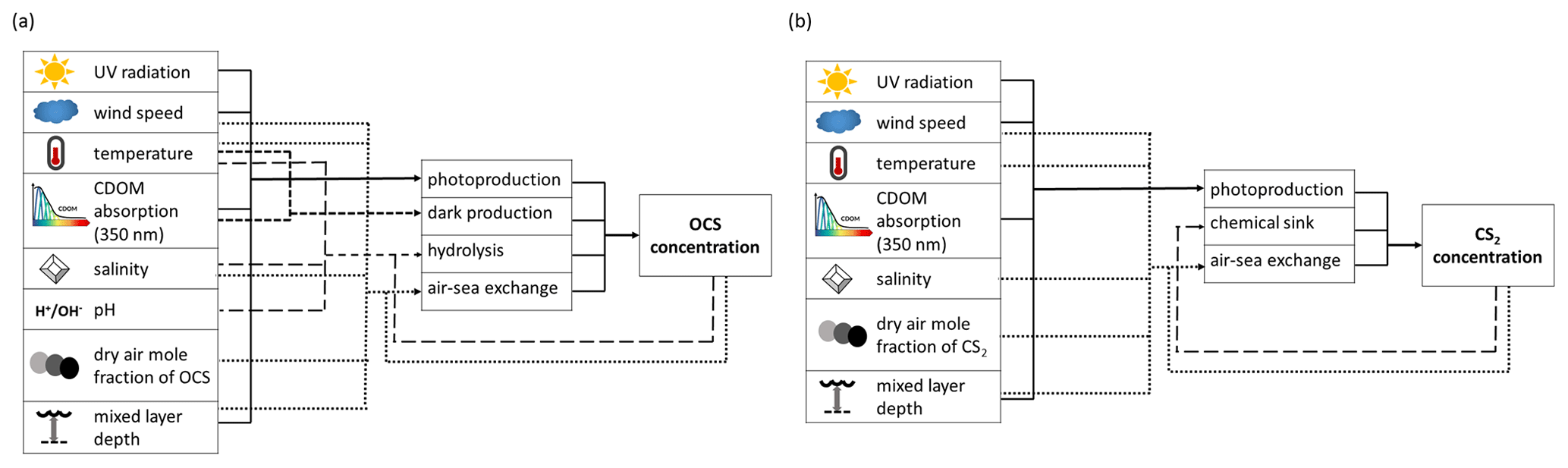
Figure 1Schematic overview of processes and forcing included in the box models for (a) OCS and (b) CS2.
CS2 is present in seawater in picomolar concentrations, and measurements are generally sparse (Lennartz et al., 2020b). A correlation between temperature and CS2 concentration in surface waters is evident across several datasets (Lennartz et al., 2019; Xie and Moore, 1999). CS2 is produced by photochemical reactions as well, following a similar shape of the AQY wavelength spectrum as OCS (Xie et al., 1998). Precursor molecules such as cysteine, cystine, methionine, and dimethyl sulphide (DMS) have been identified, and photochemical CS2 production itself seems to be temperature-dependent (Modiri Gharehveran and Shah, 2018). Furthermore, there is evidence for a biological production of CS2 by phytoplankton species, with varying yield from different species (Xie et al., 1999), but the exact mechanism is unknown. Outgassing to the atmosphere is considered the most important sink process for CS2 in the mixed layer. The only chemical sink mechanism known so far is hydrolysis, with a lifetime of several years (Elliott, 1990). However, a chemical sink process in addition to air–sea gas exchange was needed to explain observations along an Atlantic transect, with an e-folding lifetime of ca. 10 d (Kettle et al., 2001).
Here, we use existing models that include parameterizations of processes known to be relevant for each gas and apply them on a global scale, accounting for interannual variability in the forcing parameters. We present the first monthly resolved inventory for marine OCS and CS2 emissions for the period 2000–2019. The model is driven by diel cycles averaged over the course of each month or monthly averages of satellite data (Aqua MODIS for CDOM) and ERA5 reanalysis products for meteorological parameters. We encourage the community to use these emissions for atmospheric modelling studies in order to elucidate the atmospheric budget of OCS, assess variability in the supply to the sulphate aerosol layer, and determine gross primary production on a global scale (available at https://doi.org/10.5281/zenodo.4297010) (Lennartz et al., 2020a).
A model version as described in Lennartz et al. (2017) is used to model the interannual variability in oceanic emissions for OCS. A new model is developed to simulate oceanic emissions of CS2. In both models, the surface ocean is divided into grid boxes of at the Equator (T42 grid, Gaussian grid with ∼ 310 km resolution at Equator; NCAR, 2017) that comprise various depth layers of 1m thickness depending on the depth of the mixed layer in each grid box. Note that the model does not resolve physical transport between the boxes (see Lennartz et al., 2017, for details).
The numerical model simulating OCS seawater concentration and air–sea exchange (positive for flux from ocean to atmosphere) includes the processes photochemical production, light-independent production (termed “dark production”), degradation by hydrolysis, and air–sea exchange across the sea surface. The process rates are calculated as depicted in Fig. 1 based on meteorological (global radiation, wind speed, skin temperature) and physicochemical data (salinity, seawater pH, CDOM absorption, and dry mole air fraction). The processes photochemical production , dark production , hydrolysis , and air–sea exchange are calculated according to Eq. (1), all in pmol (L ⋅ s)−1 (Fig. 1):
Photochemical production is calculated as the product of UV radiation UV (W m−2 = J (m2 ⋅ s)−1), the absorption coefficient of CDOM at 350 nm a350 (m−1), and the photoproduction rate constant p integrated over the mixed layer depth (MLD) according to Eq. (2):
The photochemical rate constant p (pmol J−1) is scaled with a350 (m−1), following a rationale suggested by von Hobe et al. (2003), which reflects that a350 can be regarded as a proxy for both photosensitizer and sulphur source across large spatial scales. The linear dependence between a350 and p is calculated based on fits to observational data from three major ocean basins as described in Lennartz et al. (2017). This wavelength-integrated approach has been shown to reproduce both local measurements from several cruises and global OCS observations (von Hobe et al., 2003; Lennartz et al., 2017). UV radiation below the sea surface is calculated according to solar radiation, zenith angle, and wind speed following von Hobe et al. (2003) as described in Lennartz et al. (2017). The light field in each 1 m depth layer is calculated by reducing the incoming short-wave radiation depending on the local absorption coefficient a350. Photochemical production is then computed for each layer individually, followed by integration over the entire mixed layer. This integration inherently assumes a well-mixed surface layer.
Dark production is calculated according to Lennartz et al. (2019). This reaction rate is an update of the original formulation by von Hobe et al. (2001), resulting in a semi-empirical relationship based on observations from a wider spatial range of observation than the initial study. In this formulation, the dark-production rate depends on temperature and a350 (m−1) (Eq. 3):
OCS hydrolysis is determined according to Elliott et al. (1989) and depends on temperature (T) and salinity (S) as well as the proton activity a (H+) (–), equivalent to 10−pH, according to Eqs. (4) and (5):
Air–sea exchange is calculated as the product of the concentration gradient between water and equilibrium concentration Δc and the transfer velocity k (m s−1) parametrized according to Nightingale et al. (2000):
The equilibrium concentration is calculated according to de Bruyn et al. (1995) based on the atmospheric dry mole fraction, where here, a fixed value is assumed (Table 1). The transfer velocity is corrected for OCS with the Schmidt number, calculated based on the molar volume according to Hayduk and Laudie (1974).
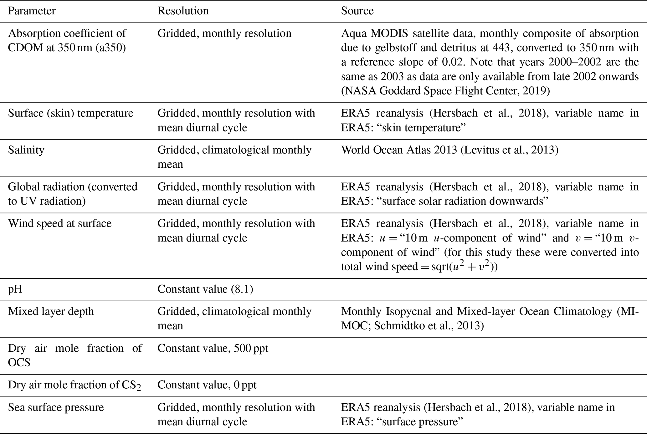
Table 1Overview of forcing parameters, their resolution, and sources used for the box model simulations in the 2000–2019 period.
The model for CS2 includes the processes of photochemical production and a first-order chemical sink (pmol (L ⋅ s)−1), according to Eq. (7).
Photochemical production is calculated in the same way as for OCS, with an additional reduction factor r (–) applied (Eq. 8).
Xie et al. (1998) approximated that CS2 photoproduction rates are about a factor of 5 smaller than OCS photoproduction rates by comparing an experimentally derived AQY from CS2 and OCS (r=0.2 in Eq. 8). The two AQYs were not measured at the same location but in comparable water properties. Another study with simultaneous measurements of both gases reported varying factors between 0.2 and 0.014 (5 to 70 times smaller than OCS photoproduction; Lennartz et al., 2019). Here, we scaled the reduction factor to obtain the best fit in the average concentration, resulting in a factor r=0.1 in Eq. (8). Thus, the model reflects the similar shape of the AQY for both gases by assuming a constant ratio, but the scaling of the overall magnitude of the photoproduction rate constant is chosen to obtain the best fit to observations from the database in Lennartz et al. (2020c). A chemical sink according to the model formulation in Kettle (2000), i.e. with an e-folding lifetime of 10 d , was implemented according to Eq. (9) (kcs in units of s−1):
Air–sea exchange was calculated as described for OCS, using the CS2 solubility according to De Bruyn et al. (1995).
As CS2 cycling in the water column is not yet well understood, this model should be understood as a base model to be extended as soon as additional process rates and their dependencies become available.
Simulations are performed for the period 2000–2019. There are several changes in the forcing data compared to the climatological run in Lennartz et al. (2017). Here we use monthly resolved data for the period 2000–2019 for a350, surface short-wave radiation, surface (skin) temperature, wind speed, and sea level pressure (Table 1). Skin temperature (diagnosed close to the air–sea interface) is used as forcing data for all temperature-relevant processes, i.e. air–sea exchange, but also dark production and hydrolysis. To test the sensitivity of emissions to the choice between skin and sea surface temperature, we performed a sensitivity test for the year 2000. The meteorological data were obtained from the ERA5 reanalysis (more specifically, its product line “ERA5 hourly data on single levels from 1979 to present”; Hersbach et al., 2018) through the Copernicus Climate Change Service (https://climate.copernicus.eu/, last access: 19 July 2020). One file per year and parameter, containing hourly data at resolution, was downloaded.
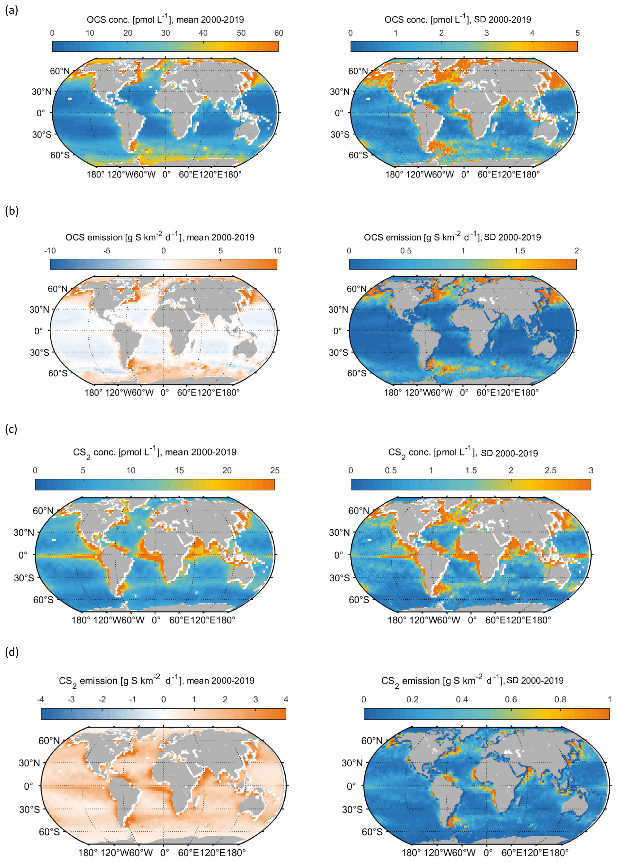
Figure 2Spatial variation, averaged over the 2000–2019 period, in (a) mean OCS surface concentration (left panel) and standard deviation of annual mean concentrations (right panel), (b) same for OCS emissions, (c) same for CS2 surface concentration, (d) same for CS2 emissions.
For wind speed, the zonal and meridional components of wind speed at 10 m altitude (m s−1) (u10 and v10, respectively) were downloaded separately and converted into wind speed (ws) according to
The post-processing of the meteorological data was done using CDO (climate data operator) tools (version 1.9.8) (Schulzweida, 2019) and comprised the following steps:
- a.
The yearly files for each parameter were split into monthly files using the CDO flag “splityearmon”, resulting in 240 monthly files covering the 20-year period 2000 to 2019 for each parameter.
- b.
For each of the 240 months within the period, monthly mean diel cycles of each meteorological parameter x were calculated using the CDO flag “dhouravg”, which calculates multi-day averages for every hour of a day as
where m is the month (1 to 12), h is the hour of the day (1 to 24), d is the day of the month (1 to 28, 29, 30, or 31), and Nm is the number of days within month m.
- c.
The resulting fields were regridded from the regular longitude–latitude grid into the spectral T42 grid (∼ ) using the CDO flag “remapcon2”, which is a second-order conservative remapping method that takes into account all source grid points, in both longitude and latitude directions. The spatial resolution is the same as in Lennartz et al. (2017). Among the remapping methods available in CDO, “remapcon2” was considered the most appropriate to interpolate the selected meteorological parameters from a fine grid to a much coarser grid. Monthly forcing fields for CDOM are derived from Aqua MODIS satellite level 3 product “absorption due to gelbstoff and detritus at 443 nm” (NASA Goddard Space Flight Center, 2019) and converted to 350 nm with an exponential slope of 0.02 for the wavelength spectrum. Climatological values are used for salinity and mixed layer depth at a monthly resolution, which is the same for each month of the year throughout the simulation period, unchanged compared to Lennartz et al. (2017). The average diel cycle of each meteorological dataset (wind, pressure, skin temperature, and solar radiation) is used for the 15th of each month (one value for every 2 h). In between, data are interpolated separately for each time of the day, resulting in a continuous change in the amplitude of the diel cycles. This procedure avoids sharp changes as if a mean monthly cycle were used for each day of the month while still being computationally effective. The initial concentration for both gases was taken as a constant value of 8 pmol L−1 in all grid boxes. The time step in the model is 2 h. The model is spun up for 1 year, repeating the conditions of the year 2000 prior to the simulation period. Maps were created using the m_map package v1.4k (Pawlowicz, 2020).
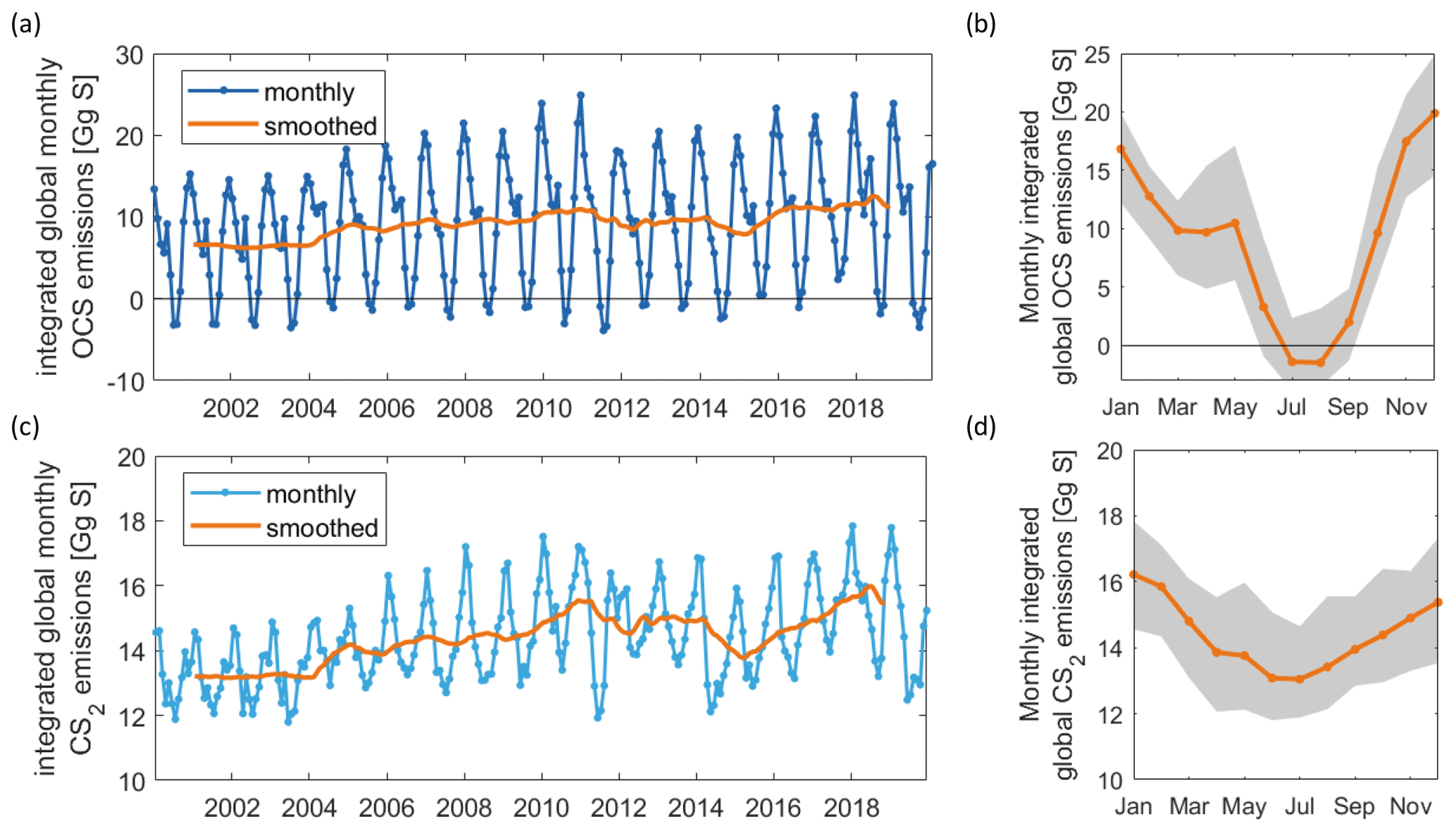
Figure 3Interannual variability in OCS emissions as time series (a) and mean annual cycle in orange, standard deviation of respective month in the shaded grey area (b). Panels (c) and (d) are the same as (a) and (b) but for CS2. The model output is saved in 2 h intervals for the 15th of each month and integrated over 30 d for the monthly emissions shown here.
4.1 Spatial and seasonal variability
Both gases show distinct spatial patterns in their annual concentration and emission averages, which reflect their marine cycling. For OCS, the highest concentrations are present in cold, high-latitude waters and shelf areas, whereas the lowest concentrations prevail in warm, subtropical gyres where CDOM abundance in the water is low (Fig. 2a). A latitudinal gradient with higher concentrations in high latitudes and low concentrations in tropical and subtropical waters reflects the temperature-dependent degradation by hydrolysis. The degradation is strongest in warm waters, where the lifetime of OCS is on the order of hours, keeping concentrations low. This general pattern is in broad agreement with observations of the largest available database on seaborne OCS measurements (Lennartz et al., 2020c). Annual mean emissions largely follow the spatial pattern of OCS seawater concentrations, with sources, i.e. flux from the ocean to the atmosphere, in shelf areas and high latitudes and sink regions in the subtropical gyres (Fig. 2b). This general source and sink pattern does not change in all years covered in this period, but the absolute concentrations and, hence, the magnitude of the emissions show variability (see Sect. 4.2). The concentration pattern follows the seasonal pattern of radiation that drives photochemical production, resulting in an annual cycle with the highest concentrations and emissions in temperate northern latitudes in boreal summer and the highest concentrations and emissions in the Southern Ocean in austral summer. The globally integrated monthly emissions are highest in austral summer and lowest in austral winter. The high emissions in the Southern Ocean outweigh the northern-hemispheric summer emissions due to the Southern Ocean’s large surface area, high wind speeds, and high OCS seawater concentrations. The amplitude of the mean seasonal cycle of OCS emissions is 21 Gg S yr−1 (Fig. 3b). In July and August, the globally integrated net emissions are close to zero, similar to a previous budget using a similar model (Kettle et al., 2002).
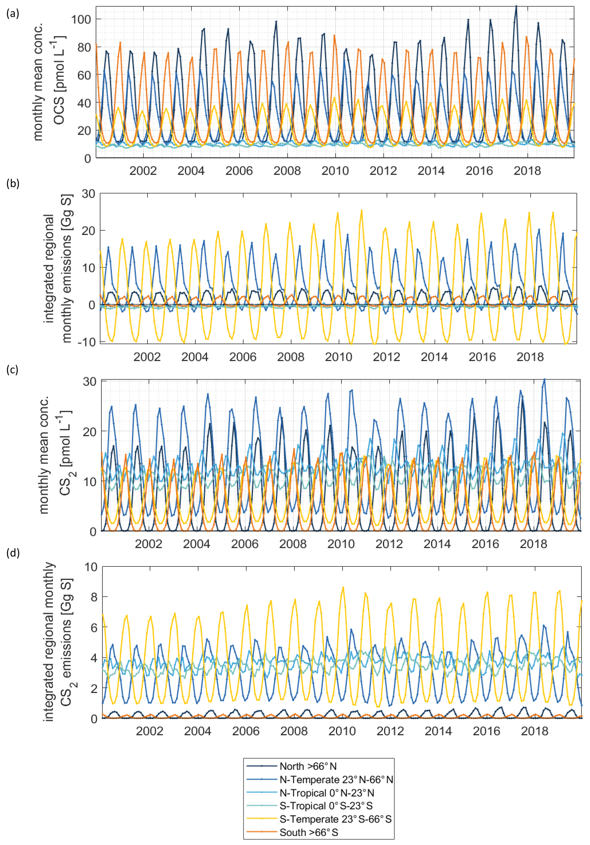
Figure 4Regionally resolved interannual variability in concentrations (a) and emissions (b) for OCS. Same in (c) and (d) for CS2.
CS2 concentrations show a different global pattern than OCS concentrations. CS2 concentrations and emissions have hotspots in coastal and shelf regions as well as in tropical and subtropical oceans, reflecting photoproduction as the main production process in the model. The tropical and subtropical areas show comparably low CS2 concentrations (Fig. 4c), and their importance for globally averaged emissions mainly comes from the large oceanic surface area (Fig. 4d). Notably, CS2 emissions in the western Pacific, where inverse modelling studies have located the missing OCS source, are relatively low (Glatthor et al., 2015; Kuai et al., 2015b). The hotspots being located in the tropical and subtropical regions with similar intensities of incoming radiation all year leads to less seasonal variation in globally integrated emissions, i.e. an amplitude of 3.2 Gg S yr−1. The ocean is a source of CS2 to the atmosphere over the entire year since emissions are calculated with an atmospheric mixing ratio of 0 ppt. This assumption is a simplification, the average of the sparse dataset (less than a thousand measurements) on CS2 air mixing ratios being 42±24 ppt but ranging to undetectable in remote ocean regions. The difference can be up to 30 % in the computed flux, similar to the uncertainty inherent to the computation of the transfer velocity. In general, the highest emissions occur in boreal winter and the lowest in boreal summer.
Table 2Globally integrated annual emissions of OCS and CS2 for each year in 2000–2019, together with descriptive statistics and trends.
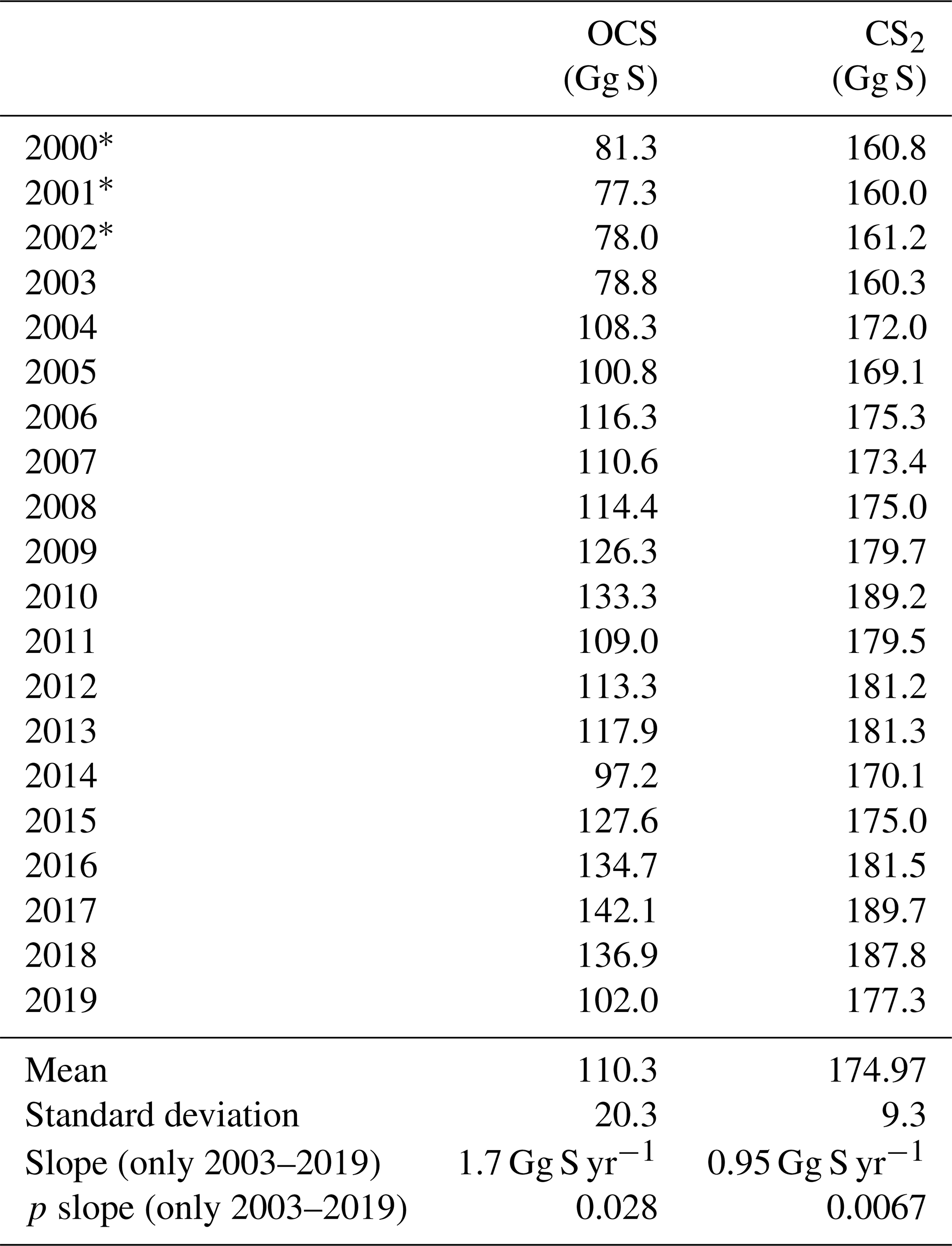
* CDOM from 2003.
4.2 Interannual variability
Surface concentrations of OCS show a similar spatial pattern across the period of 2000 to 2019, with interannual variability in the absolute concentration and, hence, emissions. Globally integrated emissions range from 77.3 Gg S yr−1 in 2001 to 142.1 Gg S yr−1 in 2017, with a mean of 110.3±20.3 Gg S yr−1 (Table 2). A significant increasing trend (p=0.028) of about 1.7 g S yr−1 is present in oceanic emissions from the period 2003–2019 (Table 2). This trend is present also in the area-weighted average sea surface concentration (slope = 0.007 pmol L−1 yr−1, ). Note that for the trend analysis, we considered only the period 2003–2019 as CDOM seems to be one of the most important drivers of interannual variability (see below), and CDOM data are only available from 2003 onwards. Generally, the seasonal variability in OCS emissions is larger (range of mean annual cycle of 21 Gg S yr−1) than the interannual variability (mean monthly variability of 8.4 Gg S per month) (Fig. 3). Interannual variability in the emissions in each month is largest during boreal spring (April, May, June) and autumn (October) (Fig. 3a). These months show the largest difference between minima and maxima during the whole period (grey area in Fig. 3a). The spatial pattern of interannual variability in OCS emissions shows the highest variability, i.e. the highest standard deviation among annual averages in each grid box, at locations with high OCS concentrations and emissions (Fig. 2). These regions comprise the northern temperate and polar regions; the Southern Ocean; and shelf areas; especially those close to coastal upwelling regions and river plumes (Fig. 2). The standard deviation for OCS concentrations between annual averages ranges from 0.22 at the oligotrophic gyres to 143.8 pmol L−1 at the highly dynamic coast off Alaska, USA (average standard deviation of 3.4 pmol L−1). The interannual variability also shows latitudinal differences. Polar regions in both Arctic and Antarctic waters display the largest seasonal cycles in OCS concentration, i.e. the highest annual variability (Fig. 4), and at the same time also display the highest interannual variability. Differences in mean concentrations (area-weighted) in summer range between 72.8 pmol L−1 in June 2011 and 91.6 pmol L−1 in July 2017, i.e. ca. 20 pmol L−1 in the Arctic Ocean (Fig. 4). Interannual differences in mean monthly OCS concentrations become smaller with decreasing latitudes and are lowest in tropical oceans, where they range between 7.0 pmol L−1 in April 2002 and 8.5 pmol L−1 in April 2018 (southern tropical) and between 8.6 pmol L−1 in June 2015 and 9.0 pmol L−1 in June 2018 (northern tropical). Due to their large surface area and medium surface OCS concentrations, southern temperate regions (23–66∘ S) have the largest integrated OCS emissions, followed by northern temperate regions (33–66∘ N) (Fig. 4). In temperate regions, the largest interannual variability occurs during the months of maximum positive emissions, with a range from 17.4 to 26.1 Gg S per month in southern temperate regions in December and from 14.0 to 20.9 Gg S per month in northern temperate regions in May. In summary, OCS concentrations and emissions show the highest interannual variability at times and locations where concentrations are high and in systems that are inherently highly dynamic, such as shelf regions.
Carbon disulphide concentrations are highest in shelf areas in the tropics and subtropics and generally decrease towards high latitudes (Fig. 2c). The spatial pattern of the annually integrated emissions mirrors this picture (Fig. 2d). While the spatial pattern of concentrations and emissions is similar in each year, the absolute concentration and magnitude of emissions does show interannual variability (Fig. 3b). Emissions are calculated here with a boundary layer mixing ratio of zero (maximum possible emission) as is commonly done for other short-lived gases such as DMS (Lana et al., 2011), so the ocean is a CS2 source at every location throughout the year. Globally integrated emissions range from 160.0 Gg S yr−1 in 2002 to 189.7 Gg S yr−1 in 2017 (Table 2). Similar to OCS, an increasing trend of global CS2 emissions for the period 2003–2019 is significant (p= 0.0067). Emissions increase with 0.95 Gg S yr−1 on average over the period 2003–2019. For globally integrated emissions, annual variability (mean range of 3.2 Gg S per month) is comparable to the interannual variability (3.2 Gg S yr−1). This is different to OCS, where annual variability was higher than interannual variability for globally integrated emissions. This difference is caused by the location of the respective hotspots of the produced gases: as OCS has its concentration and emission hotspots mainly in high latitudes, which experience a very seasonal light regime, its annual variability is high. The low concentrations of OCS (and corresponding low emissions) in the tropics result from the fast degradation by hydrolysis. In contrast, CS2 has its concentration and emission hotspots mainly in low latitudes with more constant forcing and hence displays smaller annual variability. The interannual variability in CS2 emissions among single months has a similar magnitude throughout the year (grey shaded area in Fig. 3d). Maximum monthly mean concentrations of CS2 vary the most in the summer months of the northern temperate regions (23–66∘ N), from 4.3 Gg S per month in June 2011 to 6.0 Gg S per month in June 2018, but show less variability in the winter months, i.e. between 0.8 and 1.2 Gg S per month in December. Due to their comparably low surface area and the relatively low concentrations, high-latitude regions do not play a significant role in globally integrated CS2 emissions (Fig. 4). The dominance of southern temperate emissions of CS2, despite higher absolute mean concentrations in northern temperate regions, is explained by the larger surface ocean area in the southern temperate regions (Fig. 4c and d).
4.3 Main drivers of interannual variability
The interannual variability in OCS and CS2 concentrations and emissions is a result of the interannual variability in their production and consumption processes, which in turn depend on environmental conditions. The variability comprises years like 2015 or 2017, in which positive OCS emissions occur in every month of the year, and years like 2019, where global net uptake by the ocean is present in 4 of the 12 months (Fig. 3a). Most of the interannual variability in these emissions is driven by the emissions in the high latitudes. For example, in 2017, emissions in the Arctic regions are higher than average and lead to an overall increase in the emissions even in the winter months. El Niño was strong in 2015/2016, and decreased upwelling of cold water with high CDOM content would expectably lead to low OCS emissions due to decreased photochemical and dark production and increased hydrolysis due to warmer water temperatures. However, as fluxes in the tropics are generally small, the global emissions are not substantially lower compared to other years (for 2015 they are even higher due to higher emissions in high latitudes). The many negative fluxes in 2019 seem to result from lower-than-average emissions in the Southern Ocean.
Table 3Explained variance (Pearson's R2) and significance level p for correlations of globally integrated emissions for OCS and CS2 with global annual averages of CDOM a350, skin temperature, and wind speed. Significant results (α=0.01) are indicated in bold font.
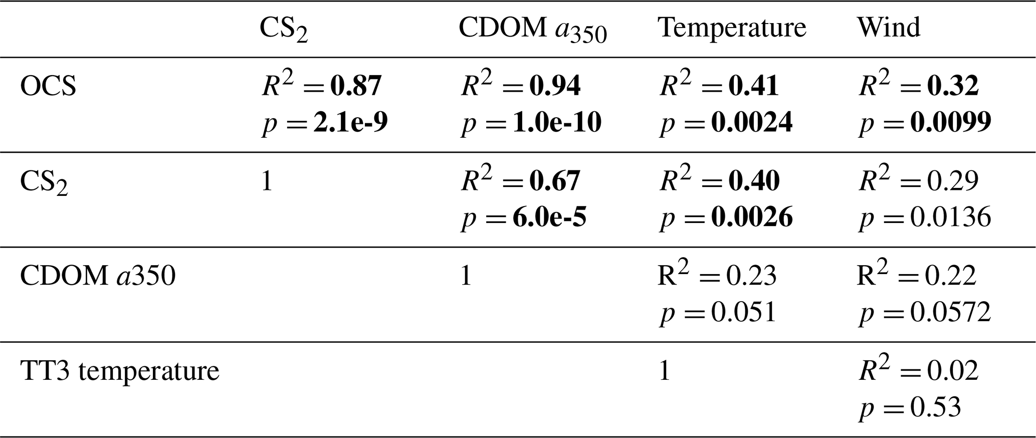

Figure 5Mean and standard deviation (maps) and interannual variation (right panels) of model input parameters: (a) CDOM a350, (b) skin temperature, (c) wind speed. Data sources listed in Table 1.
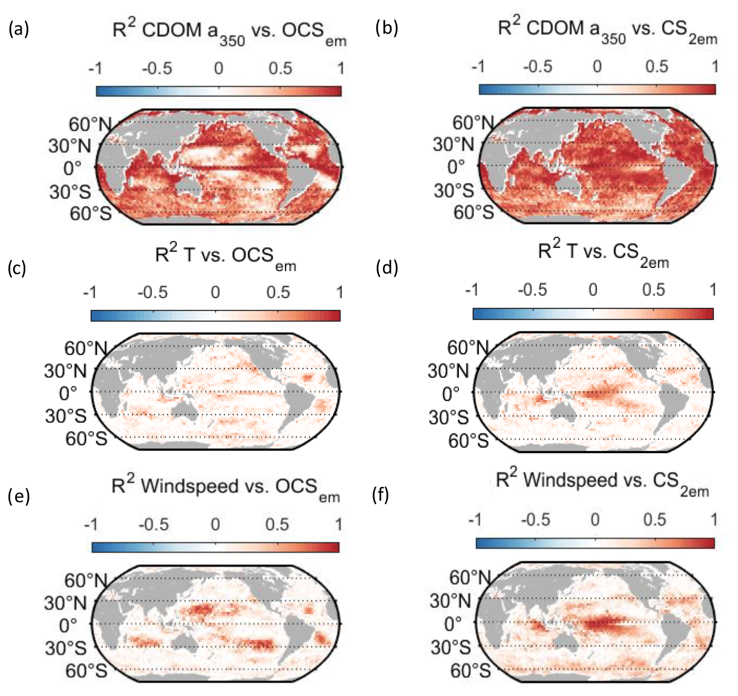
Figure 6Regional correlation of annual OCS (a, c, e) and CS2 (b, d, f) emission data with monthly data for temperature (a, b), wind speed (c, d), and CDOM absorption coefficient (e, f). Correlation is shown as Pearson's R2.
Globally integrated annual emissions of OCS correlate significantly with global annual averages (area-weighted) of CDOM a350, skin temperature, and wind speed (Table 3). CDOM a350 explains the largest variance, and sea surface temperature and wind speed explain less of the observed variance. Thus, CDOM a350 has the strongest influence on the variability in global-scale OCS concentrations. The influence is not surprising as CDOM a350 impacts both photochemical and dark production of OCS and modulates the light field in the water (at higher a350, photoproduction is higher but also more limited to the surface). The photochemical-production rate has second-order dependence on CDOM a350, reflecting its double role as photosensitizer, i.e. those molecules absorbing light energy for photochemical reactions, and as a proxy for the amount of sulphur molecules able to form radicals in photochemical reactions. As such, CDOM a350 exerts a strong, non-linear and positive influence on OCS concentration, and seems to be the main driver of its interannual variability. The overall strong influence of CDOM a350 on OCS interannual variability is also underlined by similarity in the spatial pattern of the standard deviation in annual average concentrations and emissions between OCS and CDOM a350 (Fig. 5). Sea surface temperature strongly influences OCS hydrolysis, which leads to low concentrations in warm tropical and subtropical waters. Temperature also controls the solubility of the gas in water, i.e. the equilibrium water concentration is higher in colder waters. Variations in temperature explain a small part of interannual variations in OCS emissions. However, rising temperature towards the end of the period (Fig. 5) did not outweigh the increase in CDOM a350,which supports the above-mentioned result that the observed changes in CDOM a350 had a stronger influence on overall OCS production than observed temperature changes had on hydrolysis. Finally, wind speed imposes a non-linear control on OCS emissions, but the impact is smaller than that of CDOM a350.
Resolving the correlations regionally shows distinct controls on interannual variability for CDOM and wind speed but not for temperature (Fig. 6). The highest Pearson's correlation coefficients (R2) for CDOM and OCS emissions are found globally except in the subtropical gyres (Fig. 6a). In those gyre regions, CDOM concentration is generally low (Fig. 5a), so other drivers like wind speed seem to have a higher impact on the variability (Fig. 6e). Correlations with temperature show no clear spatial pattern (Fig. 6c).
Globally integrated CS2 emissions correlate significantly with CDOM a350, with a substantial part of the variance in interannual variability (67 %) explained by this single factor, although this is less than for OCS. Photochemical production of CS2 is similarly calculated as that for OCS and hence depends non-linearly and positively on CDOM a350. The lesser amount of explained variance compared to OCS may result from the lack of a CDOM a350-dependent dark-production process. Interestingly, CS2 emissions correlate with temperature, although temperature is not part of any production or consumption process in the model and solely modulates the solubility of CS2. Increasing temperature decreases the solubility and would lead to a lower surface water concentration; hence, this effect cannot explain the correlation between temperature and CS2 surface ocean concentrations in observations (Lennartz et al., 2020). Potentially, the covariation of temperature with radiation dose might be responsible for the correlation of CS2 concentration and temperature that is evident across observational datasets (see Introduction). The spatial variation in the standard deviation of annual averages of CS2 concentration and emissions resembles that of CDOM a350, again underlining that this is a major factor for interannual variability in CS2 (Fig. 5). Regional analysis of correlations of CS2 emissions with biogeochemical and meteorological data shows that CDOM is a globally homogeneous driver of emissions, as indicated by the high Pearson's correlation coefficients globally. Temperature and wind speed show the highest correlation to CS2 emissions in the tropical West Pacific, where the assumed source region of the “missing source” of OCS is located. In these regions, interannual variability in wind speed is highest (Fig. 5), and temperature shows increased variability there (Fig. 5). This increased variability might explain the regionally strong correlation with CS2 emissions.
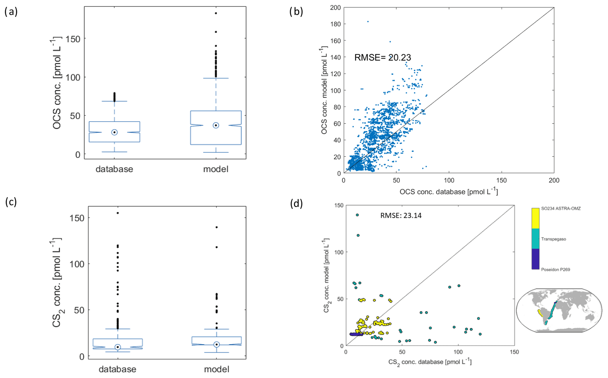
Figure 7Comparison of model output to observations from the database described in Lennartz et al. (2020). (a) Box plot of OCS reference data from database and subsampled model output at the time and location of measurements (32 cruises), (b) scatter plot of 1 : 1 comparison with the same data as in (a). The black line is the 1 : 1 line, and (c) and (d) are the same as (a) and (b) but for CS2 (three cruises).
4.4 Comparison to observations
The model output of the monthly resolved simulation for 2000–2019 is compared to the database compiled by Lennartz et al. (2020), which contains 2970 fully georeferenced OCS measurements and 501 fully georeferenced CS2 measurements in the period considered here. The model output is subsampled at the time (including time of day) and location closest to the measurements in the respective period for a 1 : 1 comparison.
For OCS, the range of the subsampled model output agrees well with data from the database (seven cruises, n=2971), with a slight underestimation of measured concentrations by the model (average of 40.1 pmol L−1 in the database, 38.4 pmol L−1 in the model; Fig. 7a). The direct comparison reveals remaining scatter around the 1 : 1 line and a high bias in the model which grows with increasing OCS concentrations (Fig. 5b). A correction for this bias was obtained from a linear fit through the 1 : 1 comparison (blue dots in Fig. 7) and yields the equation [OCS corrected] = 0.83 × [OCS modelled] − 0.7. Because the bias is still within the scatter of the data, we did not apply this correction factor in the analysis presented here. The scatter and high bias in the data likely result from simplifications in the model. The main simplifications, probably causing these discrepancies between observations and models, are the missing horizontal transport, the use of averaged wind speed as forcing, the use of CDOM a350 as a proxy for photochemical production, and the application of a climatological mean for the depth of the mixed layer.
Using CDOM a350 as a proxy for OCS photochemical production may introduce some scatter but likely not a systematic bias. The very complex nature of the dissolved organic matter pool in the ocean, which comprises CDOM as the optically active fraction, makes it difficult to assign one photoproduction rate constant or apparent quantum yield to all the reactions taking place with different precursors. CDOM a350 has been shown to be a suitable proxy across three major ocean basins (Atlantic, Pacific, and Indian oceans), but the rate constant–CDOM a350 relationship showed some scatter that might be improved when more data become available.
The missing horizontal transport can lead to a systematic model bias, especially in cold waters, where the OCS lifetime increases to timescales (days) relevant for physical transport, while environmental conditions might vary on shorter timescales. But still this process is unlikely to decouple OCS concentrations from its drivers like CDOM and temperature, which would be transported accordingly. Due to the short OCS lifetime in water, the effect of horizontal transport is negligible in warm waters of the tropics, subtropics, and most of the temperate regions. In regions with deep mixed layers such as the Southern Ocean, the assumption of a completely well-mixed surface layer may be violated and cause discrepancies between the modelled value (average of the mixed layer) and the measured value (close to the surface, i.e. higher concentration than at the bottom of the mixed layer). Since the modelled concentration depends on the depth of the mixed layer and its relation to the photic zone, a climatological average as used here will introduce biases; however, detailed information on mixed layer depth at monthly resolution from observations is not available. This simplification mainly affects OCS concentrations in high latitudes, where concentrations are relatively high, and thus might be partly responsible for the systematic bias revealed by the scatter plot in Fig. 5b. Furthermore, averaging wind speed to a mean monthly cycle will most likely lead to an underestimation of emissions and, hence, an overestimation of concentrations. Due to the non-linear relationship of the transfer velocity of the gas exchange with wind speed, averaging disproportionally reduces the effect of increased emissions during high wind speeds. Another source of uncertainty are the forcing data, e.g. the choice of using the skin temperature rather than the sea surface data. For comparison, we performed a shorter simulation covering the year 2000 and using the ERA5 sea surface temperature data instead of the skin temperature. The difference in resulting global emissions was 1.2 %, i.e. very small compared to other uncertainties. Still, given these simplifications and assumptions, the overall good agreement with the measurements underlines the applicability of the model for assessing the marine cycling of OCS and its emissions to the atmosphere.
The marine cycling of CS2 is less well understood than that of OCS. This relatively poorer process understanding is reflected by the comparison of the modelled CS2 concentrations with those of the database (3 cruises, 501 measurements) (R2=0.04). Modelled concentrations agree with observations on average (average database: 18.0 pmol L−1; average subsampled model output: 18.2 pmol L−1). The three cruises cover the Mauritanian upwelling (Poseidon 269; blue in Fig. 7d), the Peruvian upwelling (ASTRA-OMZ; yellow in Fig. 7d), and a transect through the Atlantic (Transpegaso; green in Fig. 7d). As such, they cover a broad range of different biogeochemical regimes, but regions such as oligotrophic gyres or high-latitude waters are not covered; i.e. a substantial part of the global variability might be missing in the reference dataset. While the cruises Poseidon 269 and ASTRA-OMZ are relatively well represented by the model (colour code in Fig. 7d), the variability in the measurements during Transpegaso is not well captured. The model used here has some underlying assumptions and simplifications that call for refinement in the future when detailed process understanding is available. For example, the model is based on the assumption of a constant ratio between the apparent quantum yields of OCS and CS2. It has been shown that this ratio is not always constant (Kettle, 2000; Lennartz et al., 2019), but as the production pathways of both gases show some similarities (Modiri Gharehveran and Shah, 2018), the model formulation with a constant ratio is a first approximation. Second, the presence of a chemical sink is rationalized by its necessity to explain observed concentrations along an Atlantic transect (Kettle, 2000; Lennartz et al., 2019) but has no mechanistic foundation so far. Dedicated laboratory experiments disentangling the source and sink processes in the water column are needed to further resolve this issue and to improve modelling efforts. Finally, this model does not consider any biological production of CS2. This assumption is justified for a first approximation as CDOM and primary production (photosynthesis) show similar global-scale patterns. High CDOM will thus lead to high production of CS2 in the water, even though the scaling of the photoproduction rate constant (AQY) might inherently include biological production due to the covariation of photosynthesis patterns with CDOM and radiation. The calculated CS2 emission estimate is not sensitive to the choice of the temperature forcing data; the resulting differences in global emissions when using the sea surface temperature instead of the skin temperature for the year 2000 resulted in a negligible deviation of 0.12 %. Overall, the presented CS2 concentration and emissions are a first approximation, and more detailed process understanding is important to improve emission estimates. Assuming that the presented oceanic emissions are in a realistic range, the calculated emissions would not be enough to close the gap in the atmospheric budget of OCS on the order of 600 to 800 Tg S yr−1 (Berry et al., 2013; Glatthor et al., 2015; Kuai et al., 2015a) given that only a little more than half of the sulphur in CS2 is converted to sulphur in OCS.
The emission estimate of the gases OCS and CS2 includes further uncertainties introduced by the parameterizations of the transfer velocity used for calculation of air–sea exchange, which carry large uncertainties, especially at high wind speeds (Wanninkhof, 2014). Furthermore, emissions here are calculated based on the concentration gradient between surface water and the equilibrium concentration dictated by the atmospheric mixing ratio without taking into account any potential effect of the sea surface microlayer. Whether and how the enrichment of surfactants in the sea surface microlayer affects emissions of these gases has not been sufficiently assessed to date.
The code is available on GitHub under https://github.com/Sinikka-L/OCS_CS2_boxmodel (Lennartz, 2020). The simulation output is available at Zenodo (https://doi.org/10.5281/zenodo.4297010) (Lennartz et al., 2020a). The output consists of one netCDF file for each gas, each of a size of ca. 444 MB, with monthly averages of sea surface concentrations and emissions to the atmosphere as well as a mean diel cycle for each month.
OCS and CS2 are climate-relevant trace gases, and OCS can also be used as a proxy to infer terrestrial gross primary production. A missing source in the atmospheric OCS budget currently makes conclusions on the future impact on both gases and the application of this proxy on a global scale difficult. Since both gases contribute to the atmospheric OCS budget, their oceanic emissions have been suggested previously to account for that missing source. We provide monthly resolved OCS and CS2 concentration and marine emission data for the period 2000–2019 based on a mechanistic ocean box model. We show that interannual variability in OCS is smaller than its seasonal variability in globally integrated emissions but that a significant positive trend is evident across the period 2000–2019. The main driver for interannual variabilities is variation in CDOM a350. The comparison of our data to a database with more than 2500 measurements reveals an overall good agreement. The CS2 model presented here for the first time is a first approximation and reveals stronger interannual variability than seasonal variability in emissions. Again, CDOM (or, indirectly, biological production) seems to strongly influence concentration and emission patterns of CS2. Similarly, an increasing trend in CS2 emissions is significant for the period 2000–2019. Based on the data presented here, it seems unlikely that the missing atmospheric source of 600–800 Gg S yr−1 (Berry et al., 2013; Glatthor et al., 2015; Kuai et al., 2015a) might be balanced by tropical marine emissions of OCS or CS2. We encourage the use of the data provided here as input for atmospheric modelling studies to further assess the atmospheric OCS budget and the role of OCS in climate.
STL and MG conceived the study with input from MvH and CAM. MG prepared meteorological forcing data for the model simulations. STL performed the simulations and evaluated data jointly with MG, MvH, and CAM. STL wrote the manuscript with contributions from all coauthors.
The authors declare that they have no conflict of interest.
This article is part of the special issue “Surface emissions for atmospheric chemistry and air quality modelling”. It is not associated with a conference.
The authors thank the Ocean Biology and Processing Group at NASA Goddard Space Flight Center for access to the Aqua MODIS data as well as ECMWF and the Copernicus Climate Change Service for access to the ERA5 data.
This paper was edited by Nellie Elguindi and reviewed by two anonymous referees.
Berry, J., Wolf, A., Campbell, J. E., Baker, I., Blake, N., Blake, D., Denning, A. S., Kawa, S. R., Montzka, S. A., Seibt, U., Stimler, K., Yakir, D., and Zhu, Z.: A coupled model of the global cycles of carbonyl sulfide and CO 2: A possible new window on the carbon cycle, J. Geophys. Res.-Biogeo., 118, 842–852, https://doi.org/10.1002/jgrg.20068, 2013.
Brühl, C., Lelieveld, J., Crutzen, P. J., and Tost, H.: The role of carbonyl sulphide as a source of stratospheric sulphate aerosol and its impact on climate, Atmos. Chem. Phys., 12, 1239–1253, https://doi.org/10.5194/acp-12-1239-2012, 2012.
De Bruyn, W. J., Swartz, E., Hu, J. H., Shorter, J. A., Davidovits, P., Worsnop, D. R., Zahniser, M. S., and Kolb, C. E.: Henry's law solubilities and Śetchenow coefficients for biogenic reduced sulfur species obtained from gas-liquid uptake measurements, J. Geophys. Res., 100, 7245–7251, https://doi.org/10.1029/95JD00217, 1995.
Chin, M. and Davis, D. D.: Global sources and sinks of OCS and CS 2 and their distributions, Global Biogeochem. Cy., 7, 321–337, https://doi.org/10.1029/93GB00568, 1993.
Cutter, G. A. and Radford-Knoery, J.: Carbonyl sulfide in two estuaries and shelf waters of the western North Atlantic Ocean, Mar. Chem., 43, 225–233, https://doi.org/10.1016/0304-4203(93)90228-G, 1993.
Cutter, G. A., Cutter, L. S., and Filippino, K. C.: Sources and cycling of carbonyl sulfide in the Sargasso Sea, Limnol. Oceanogr., 49, 555–565, https://doi.org/10.4319/lo.2004.49.2.0555, 2004.
EEA 1/2017: Climate Change, impacts and vulnerability in Europe 2016 – an indicator based report, Copenhagen, Denmark, 2017.
Elliott, S.: Effect of hydrogen peroxide on the alkaline hydrolysis of carbon disulfide, Environ. Sci. Technol., 24, 264–267, https://doi.org/10.1021/es00072a017, 1990.
Elliott, S., Lu, E., and Rowland, F. S.: Carbonyl sulfide hydrolysis as a source of hydrogen sulfide in open ocean seawater, Geophys. Res. Lett., 14, 131–134, https://doi.org/10.1029/GL014i002p00131, 1987.
Elliott, S., Lu, E., and Rowland, F. S.: Rates and mechanisms for the hydrolysis of carbonyl sulfide in natural waters, Environ. Sci. Technol., 23, 458–461, https://doi.org/10.1021/es00181a011, 1989.
Ferek, R. J. and Andreae, M. O.: The supersaturation of carbonyl sulfide in surface waters of the Pacific Ocean off Peru, Geophys. Res. Lett., 10, 393–396, https://doi.org/10.1029/GL010i005p00393, 1983.
Ferek, R. J. and Andreae, M. O.: Photochemical production of carbonyl sulphide in marine surface waters, Nature, 307, 148–150, https://doi.org/10.1038/307148a0, 1984.
Glatthor, N., Höpfner, M., Baker, I. T., Berry, J., Campbell, J. E., Kawa, S. R., Krysztofiak, G., Leyser, A., Sinnhuber, B.-M., Stiller, G. P., Stinecipher, J., and von Clarmann, T.: Tropical sources and sinks of carbonyl sulfide observed from space, Geophys. Res. Lett., 42, 10082–10090, https://doi.org/10.1002/2015GL066293, 2015.
Hayduk, W. and Laudie, H.: Prediction of diffusion coefficients for nonelectrolytes in dilute aqueous solutions, AIChE J., 20, 611–615, https://doi.org/10.1002/aic.690200329, 1974.
Hersbach, H., Bell, B., Berrisford, P., Biavati, G., Horányi, A., Muñoz Sabater, J., Nicolas, J., Peubey, C., Radu, R., Rozum, I., Schepers, D., Simmons, A., Soci, C., Dee, D., and Thépaut, J.-N.: ERA5 hourly data on single levels from 1979 to present, Copernicus Clim. Chang. Serv. Clim. Data Store (CDS), https://doi.org/10.24381/cds.adbb2d47, 2018.
Kamyshny, A. J., Goifman, A., Rizkov, D., and Lev, O.: Formation of Carbonyl Sulfide by the Reaction of Carbon Monoxide and Inorganic Polysulfides, Environ. Sci. Technol., 37, 1865–1872, https://doi.org/10.1021/ES0201911, 2003.
Kettle, A. J.: Extrapolations of the Flux of Dimethylsulfide, Carbon Monoxide, Carbonyl Sulfide and Carbon Disulfide from the Oceans, York University, 2000.
Kettle, A. J., Rhee, T. S., von Hobe, M., Poulton, A., Aiken, J., and Andreae, M. O.: Assessing the flux of different volatile sulfur gases from the ocean to the atmosphere, J. Geophys. Res. Atmos., 106, 12193–12209, https://doi.org/10.1029/2000JD900630, 2001.
Kettle, A. J., Kuhn, U., von Hobe, M. von, Kesselmeier, J., and Andreae, M. O.: Global budget of atmospheric carbonyl sulfide: Temporal and spatial variations of the dominant sources and sinks, J. Geophys. Res., 107, 4658, https://doi.org/10.1029/2002JD002187, 2002.
Khalil, M. A. K. and Rasmussen, R. A.: Global sources, lifetimes and mass balances of carbonyl sulfide (OCS) and carbon disulfide (CS2) in the earth's atmosphere, Atmos. Environ., 18, 1805–1813, https://doi.org/10.1016/0004-6981(84)90356-1, 1984.
Kremser, S., Thomason, L. W., von Hobe, M., Hermann, M., Deshler, T., Timmreck, C., Toohey, M., Stenke, A., Schwarz, J. P., Weigel, R., Fueglistaler, S., Prata, F. J., Vernier, J.-P., Schlager, H., Barnes, J. E., Antuña-Marrero, J.-C., Fairlie, D., Palm, M., Mahieu, E., Notholt, J., Rex, M., Bingen, C., Vanhellemont, F., Bourassa, A., Plane, J. M. C., Klocke, D., Carn, S. A., Clarisse, L., Trickl, T., Neely, R., James, A. D., Rieger, L., Wilson, J. C., and Meland, B.: Stratospheric aerosol-Observations, processes, and impact on climate, Rev. Geophys., 54, 278–335, https://doi.org/10.1002/2015RG000511, 2016.
Ksionzek, K. B., Lechtenfeld, O. J., McCallister, S. L., Schmitt-Kopplin, P., Geuer, J. K., Geibert, W., and Koch, B. P.: Dissolved organic sulfur in the ocean: Biogeochemistry of a petagram inventory, Science, 354, 456–459, https://doi.org/10.1126/science.aaf7796, 2016.
Kuai, L., Worden, J. R., Campbell, J. E., Kulawik, S. S., Li, K. F., Lee, M., Weidner, R. J., Montzka, S. A., Moore, F. L., Berry, J. A., Baker, I., Denning, A. S., Bian, H., Bowman, K. W., Liu, J., and Yung, Y. L.: Estimate of carbonyl sulfide tropical oceanic surface fluxes using aura tropospheric emission spectrometer observations, J. Geophys. Res., 120, 11012–11023, https://doi.org/10.1002/2015JD023493, 2015a.
Kuai, L., Worden, J. R., Campbell, J. E., Kulawik, S. S., Li, K.-F., Lee, M., Weidner, R. J., Montzka, S. A., Moore, F. L., Berry, J. A., Baker, I., Denning, A. S., Bian, H., Bowman, K. W., Liu, J., and Yung, Y. L.: Estimate of carbonyl sulfide tropical oceanic surface fluxes using Aura Tropospheric Emission Spectrometer observations, J. Geophys. Res.-Atmos., 120, 11012–11023, https://doi.org/10.1002/2015JD023493, 2015b.
Lana, A., Bell, T. G., Simó, R., Vallina, S. M., Ballabrera-Poy, J., Kettle, A. J., Dachs, J., Bopp, L., Saltzman, E. S., Stefels, J., Johnson, J. E., and Liss, P. S.: An updated climatology of surface dimethlysulfide concentrations and emission fluxes in the global ocean, Global Biogeochem. Cy., 25, GB1004, https://doi.org/10.1029/2010GB003850, 2011.
Launois, T., Belviso, S., Bopp, L., Fichot, C. G., and Peylin, P.: A new model for the global biogeochemical cycle of carbonyl sulfide – Part 1: Assessment of direct marine emissions with an oceanic general circulation and biogeochemistry model, Atmos. Chem. Phys., 15, 2295–2312, https://doi.org/10.5194/acp-15-2295-2015, 2015.
Lennartz, S. T.: Interactive comment on “Oceanic emissionsunlikely to account for the missing source ofatmospheric carbonyl sulfide” by Sinikka T. Lennartz et al., Atmos. Chem. Phys. Discuss., https://doi.org/10.5194/acp-2016-778-AC3, 2016.
Lennartz, S. T.: OCS_CS2_boxmodel, GitHub, available at: https://github.com/Sinikka-L/OCS_CS2_boxmodel (last access: 21 April 2021), 2020.
Lennartz, S. T., Marandino, C. A., von Hobe, M., Cortes, P., Quack, B., Simo, R., Booge, D., Pozzer, A., Steinhoff, T., Arevalo-Martinez, D. L., Kloss, C., Bracher, A., Röttgers, R., Atlas, E., and Krüger, K.: Direct oceanic emissions unlikely to account for the missing source of atmospheric carbonyl sulfide, Atmos. Chem. Phys., 17, 385–402, https://doi.org/10.5194/acp-17-385-2017, 2017.
Lennartz, S. T., von Hobe, M., Booge, D., Bittig, H. C., Fischer, T., Gonçalves-Araujo, R., Ksionzek, K. B., Koch, B. P., Bracher, A., Röttgers, R., Quack, B., and Marandino, C. A.: The influence of dissolved organic matter on the marine production of carbonyl sulfide (OCS) and carbon disulfide (CS2) in the Peruvian upwelling, Ocean Sci., 15, 1071–1090, https://doi.org/10.5194/os-15-1071-2019, 2019.
Lennartz, S., Gauss, M., von Hobe, M., and Marandino, C.: Carbonyl Sulfide (OCS/COS) and Carbon Disulfide (CS2): global modelled marine surface concentrations and emissions, 2000–2019, Zenodo, https://doi.org/10.5281/zenodo.4297010, 2020a.
Lennartz, S. T., Marandino, C. A., von Hobe, M., Andreae, M. O., Aranami, K., Atlas, E., Berkelhammer, M., Bingemer, H., Booge, D., Cutter, G., Cortes, P., Kremser, S., Law, C. S., Marriner, A., Simó, R., Quack, B., Uher, G., Xie, H., and Xu, X.: Marine carbonyl sulfide (OCS) and carbon disulfide (CS2): a compilation of measurements in seawater and the marine boundary layer, Earth Syst. Sci. Data, 12, 591–609, https://doi.org/10.5194/essd-12-591-2020, 2020b.
Lennartz, S. T., Marandino, C. A., von Hobe, M., Andreae, M. O., Aranami, K., Atlas, E., Berkelhammer, M., Bingemer, H., Booge, D., Cutter, G., Cortes, P., Kremser, S., Law, C. S., Marriner, A., Simó, R., Quack, B., Uher, G., Xie, H., and Xu, X.: Marine carbonyl sulfide (OCS) and carbon disulfide (CS2): a compilation of measurements in seawater and the marine boundary layer, Earth Syst. Sci. Data, 12, 591–609, https://doi.org/10.5194/essd-12-591-2020, 2020c.
Levitus, S., Boyer, T. P., Garcia, H. E., Locarnini, R. A., Zweng, M. M., Mishonov, A. V., Reagan, J. R., Antonov, J. I., Baranova, O. K., Biddle, M., Hamilton, M., Johnson, D. R., Paver, C. R., and Seidov, D.: World Ocean Atlas 2013 (NCEI Accession 0114815) [Salinity], NOAA Natl. Centers Environ. Information, Dataset, https://doi.org/10.7289/v5f769gt, 2013.
Modiri Gharehveran, M. and Shah, A. D.: Indirect Photochemical Formation of Carbonyl Sulfide and Carbon Disulfide in Natural Waters: Role of Organic Sulfur Precursors, Water Quality Constituents, and Temperature, Environ. Sci. Technol., 52, 9108–9117, https://doi.org/10.1021/acs.est.8b01618, 2018.
Montzka, S. A., Calvert, P., Hall, B. D., Elkins, J. W., Conway, T. J., Tans, P. P., and Sweeney, C.: On the global distribution, seasonality, and budget of atmospheric carbonyl sulfide (COS) and some similarities to CO2, J. Geophys. Res., 112, D09302, https://doi.org/10.1029/2006JD007665, 2007.
NASA Goddard Space Flight Center, Ocean Ecology Laboratory, Ocean Biology Processing Group. Moderate-resolution Imaging Spectroradiometer (MODIS) Aqua Inherent Optical Properties Data; 2018 Reprocessing. NASA OB.DAAC, Greenbelt, MD, USA, https://doi.org/10.5067/AQUA/MODIS/L3M/IOP/2018, 2019.
NCAR: The Climate Data Guide: Common Spectral Model Grid Resolutions, Natl. Cent. Atmos. Res. Staff, available at: https://climatedataguide.ucar.edu/climate-model-evaluation/common-spectral-model-grid-resolutions (last access: 3 December 2020), 2017.
Nightingale, P. D., Malin, G., Law, C. S., Watson, A. J., Liss, P. S., Liddicoat, M. I., Boutin, J., and Upstill-Goddard, R. C.: In situ evaluation of air-sea gas exchange parameterizations using novel conservative and volatile tracers, Global Biogeochem. Cy., 14, 373–387, https://doi.org/10.1029/1999GB900091, 2000.
Pawlowicz, R.: M_Map: A mapping package for MATLAB, v1.4k, available at: https://www.eoas.ubc.ca/~rich/map.html, last access: 20 August 2019.
Pos, W. H., Riemer, D. D., and Zika, R. G.: Carbonyl sulfide (OCS) and carbon monoxide (CO) in natural waters: evidence of a coupled production pathway, Mar. Chem., 62, 89–101, https://doi.org/10.1016/S0304-4203(98)00025-5, 1998.
Preiswerk, D. and Najjar, R. G.: A global, open-ocean model of carbonyl sulfide and its air-sea flux, Global Biogeochem. Cy., 14, 585–598, https://doi.org/10.1029/1999GB001210, 2000.
Rasmussen, R. A., Khalil, M. A. K., and Hoyt, S. D.: The oceanic source of carbonyl sulfide (OCS), Atmos. Environ., 16, 1591–1594, https://doi.org/10.1016/0004-6981(82)90111-1, 1982.
Schmidtko, S., Johnson, G. C., and Lyman, J. M.: MIMOC: A global monthly isopycnal upper-ocean climatology with mixed layers, J. Geophys. Res.-Ocean., 118, 1658–1672, https://doi.org/10.1002/jgrc.20122, 2013.
Solomon, S., Daniel, J. S., Neely, R. R., Vernier, J.-P., Dutton, E. G., and Thomason, L. W.: The Persistently Variable “Background” Stratospheric Aerosol Layer and Global Climate Change, Science, 333, 866–870, https://doi.org/10.1126/science.1206027, 2011.
Solomon, S., Kinnison, D., Bandoro, J., and Garcia, R.: Simulation of polar ozone depletion: An update, J. Geophys. Res.-Atmos., 120, 7958–7974, https://doi.org/10.1002/2015JD023365, 2015.
Stickel, R. E., Chin, M., Daykin, E. P., Hynes, A. J., Wine, P. H., and Wallington, T. J.: Mechanistic studies of the hydroxyl-initiated oxidation of carbon disulfide in the presence of oxygen, J. Phys. Chem., 97, 13653–13661, https://doi.org/10.1021/j100153a038, 1993.
Stimler, K., Montzka, S. A., Berry, J. A., Rudich, Y., and Yakir, D.: Relationships between carbonyl sulfide (COS) and CO2 during leaf gas exchange, New Phytol., 186, 869–878, https://doi.org/10.1111/j.1469-8137.2010.03218.x, 2010.
Suntharalingam, P., Kettle, A. J., Montzka, S. M., and Jacob, D. J.: Global 3-D model analysis of the seasonal cycle of atmospheric carbonyl sulfide: Implications for terrestrial vegetation uptake, Geophys. Res. Lett., 35, L19801, https://doi.org/10.1029/2008GL034332, 2008.
Turco, R. P., Whitten, R. C., Toon, O. B., Pollack, J. B., and Hamill, P.: OCS, stratospheric aerosols and climate, Nature, 283, 283–285, https://doi.org/10.1038/283283a0, 1980.
von Hobe, M., Cutter, G. A., Kettle, A. J., and Andreae, M. O.: Dark production: A significant source of oceanic COS, J. Geophys. Res.-Ocean., 106, 31217–31226, https://doi.org/10.1029/2000JC000567, 2001.
von Hobe, M., Najjar, R. G., Kettle, A. J., and Andreae, M. O.: Photochemical and physical modeling of carbonyl sulfide in the ocean, J. Geophys. Res., 108, 3229, https://doi.org/10.1029/2000JC000712, 2003.
Wanninkhof, R.: Relationship between wind speed and gas exchange over the ocean revisited, Limnol. Oceanogr.-Meth., 12, 351–362, https://doi.org/10.4319/lom.2014.12.351, 2014.
Watts, S. F.: The mass budgets of carbonyl sulfide, dimethyl sulfide, carbon disulfide and hydrogen sulfide, Atmos. Environ., 34, 761–779, https://doi.org/10.1016/S1352-2310(99)00342-8, 2000.
Weiss, P. S., Andrews, S. S., Johnson, J. E., and Zafiriou, O. C.: Photoproduction of carbonyl sulfide in South Pacific Ocean waters as a function of irradiation wavelength, Geophys. Res. Lett., 22, 215–218, https://doi.org/10.1029/94GL03000, 1995a.
Weiss, P. S., Johnson, J. E., Gammon, R. H., and Bates, T. S.: Reevaluation of the open ocean source of carbonyl sulfide to the atmosphere, J. Geophys. Res., 100, 23083–23092, https://doi.org/10.1029/95jd01926, 1995b.
Whelan, M. E., Lennartz, S. T., Gimeno, T. E., Wehr, R., Wohlfahrt, G., Wang, Y., Kooijmans, L. M. J., Hilton, T. W., Belviso, S., Peylin, P., Commane, R., Sun, W., Chen, H., Kuai, L., Mammarella, I., Maseyk, K., Berkelhammer, M., Li, K.-F., Yakir, D., Zumkehr, A., Katayama, Y., Ogée, J., Spielmann, F. M., Kitz, F., Rastogi, B., Kesselmeier, J., Marshall, J., Erkkilä, K.-M., Wingate, L., Meredith, L. K., He, W., Bunk, R., Launois, T., Vesala, T., Schmidt, J. A., Fichot, C. G., Seibt, U., Saleska, S., Saltzman, E. S., Montzka, S. A., Berry, J. A., and Campbell, J. E.: Reviews and syntheses: Carbonyl sulfide as a multi-scale tracer for carbon and water cycles, Biogeosciences, 15, 3625–3657, https://doi.org/10.5194/bg-15-3625-2018, 2018.
Xie, H. and Moore, R. M.: Carbon disulfide in the North Atlantic and Pacific oceans, J. Geophys. Res.-Ocean., 104, 5393–5402, https://doi.org/10.1029/1998JC900074, 1999.
Xie, H., Moore, R. M., and Miller, W. L.: Photochemical production of carbon disulphide in seawater, J. Geophys. Res.-Ocean., 103, 5635–5644, https://doi.org/10.1029/97jc02885, 1998.
Xie, H., Scarratt, M. G., and Moore, R. M.: Carbon disulphide production in laboratory cultures of marine phytoplankton, Atmos. Environ., 33, 3445–3453, https://doi.org/10.1016/S1352-2310(98)00430-0, 1999.
Zepp, R. G. and Andreae, M. O.: Factors affecting the photochemical production of carbonyl sulfide in seawater, Geophys. Res. Lett., 21, 2813–2816, https://doi.org/10.1029/94GL03083, 1994.