Development of the global dataset of Wetland Area and Dynamics for Methane Modeling (WAD2M)

Seasonal and interannual variations in global wetland area are a strong driver of fluctuations in global methane (CH₄) emissions. Current maps of global wetland extent vary in their wetland definition, causing substantial disagreement between and large uncertainty in estimates of wetland methane emissions. To reconcile these differences for large-scale wetland CH₄ modeling, we developed the global Wetland Area and Dynamics for Methane Modeling (WAD2M) version 1.0 dataset at a ∼ 25 km resolution at the Equator (0.25^∘) at a monthly time step for 2000–2018. WAD2M combines a time series of surface inundation based on active and passive microwave remote sensing at a coarse resolution with six static datasets that discriminate inland waters, agriculture, shoreline, and non-inundated wetlands. We excluded all permanent water bodies (e.g., lakes, ponds, rivers, and reservoirs), coastal wetlands (e.g., mangroves and sea grasses), and rice paddies to only represent spatiotemporal patterns of inundated and non-inundated vegetated wetlands. Globally, WAD2M estimates the long-term maximum wetland area at 13.0×10⁶ km² (13.0 Mkm²), which can be divided into three categories: mean annual minimum of inundated and non-inundated wetlands at 3.5 Mkm², seasonally inundated wetlands at 4.0 Mkm² (mean annual maximum minus mean annual minimum), and intermittently inundated wetlands at 5.5 Mkm² (long-term maximum minus mean annual maximum). WAD2M shows good spatial agreements with independent wetland inventories for major wetland complexes, i.e., the Amazon Basin lowlands and West Siberian lowlands, with Cohen's kappa coefficient of 0.54 and 0.70 respectively among multiple wetland products. By evaluating the temporal variation in WAD2M against modeled prognostic inundation (i.e., TOPMODEL) and satellite observations of inundation and soil moisture, we show that it adequately represents interannual variation as well as the effect of El Niño–Southern Oscillation on global wetland extent. This wetland extent dataset will improve estimates of wetland CH₄ fluxes for global-scale land surface modeling. The dataset can be found at https://doi.org/10.5281/zenodo.3998454 (Zhang et al., 2020).

1 Introduction

Wetlands cover about 10 % of global land area (Davidson et al., 2018) and play an important role in regulating global climate via biogeochemical cycling of greenhouse gases (IPCC, 2013). Wetlands are highly productive ecosystems that store large amounts of soil carbon due to their waterlogged conditions inhibiting aerobic soil respiration. Flooded conditions alter the soil redox state for microbes to favor methanogenesis, and thus wetlands are the largest natural source of methane (CH₄) to the atmosphere, contributing ∼ 20 %–30 % of the total annual global methane budget (Kirschke et al., 2013; Saunois et al., 2016, 2020). The spatial and temporal distribution of wetlands is one of the most important and yet uncertain factors determining the time and location of CH₄ fluxes (Melton et al., 2013; Parker et al., 2018). Wetlands are at risk from human activities such as conversion to agricultural lands and land clearing and drainage and are also at risk from climate-change-caused drying or less predictable precipitation events (Davidson et al., 2018).

Because wetland definitions vary between science, applications, and policy objectives, a definition suitable for CH₄ modeling is needed for comparative reasons and to avoid double counting. Since the first global wetland map of Matthews and Fung (Matthews and Fung, 1987), several additional global and regional wetland area datasets have been developed (Table A1). These datasets are characterized by differences in definition, data sources, methodologies, and time period covered. For example, the Ramsar Convention on Wetlands focusing on nature conservation uses an inclusive definition for wetlands as both vegetated and non-vegetated systems (i.e., rivers, lakes, ponds). However, the biogeochemistry and methane flux pathways from open water and vegetated wetlands differ substantially. Additionally, human-made water bodies (e.g., reservoirs, rice paddies, agricultural wastewater ponds, i.e., aquaculture; Grinham et al., 2018) are considered wetlands in the definition of the IPCC Guidelines for National Greenhouse Gas Inventories (Hiraishi et al., 2014). The biogeochemical processes in these kinds of intensely managed wetlands differ from those of natural wetlands, and generic modeling approaches are not applicable. Boreal taiga forests and tropical floodplains, which are considered CH₄-emitting areas given their seasonally inundated states and significant CH₄ transport pathway via tree stems (Barba et al., 2019; Pangala et al., 2017), are underestimated by many wetland mapping products (Junk, 2013) due to the lack of record in inventories and difficulty in detecting dense forest canopies in the satellite-based products. Broadly defined, wetland datasets available to this day fall into one of four types: (1) static maps based on a compilation of regional inventories based on geomorphic features and aerial photography (Finlayson et al., 1999; Hugelius et al., 2013; Lehner and Döll, 2004; Matthews and Fung, 1987; Wulder et al., 2018), (2) remote-sensing-derived products (Aires et al., 2017; Carroll et al., 2009; DeVries et al., 2017; Feng et al., 2016; Jensen and McDonald, 2019; Papa et al., 2010; Pekel et al., 2016; Poulter et al., 2017; Prigent et al., 2001, 2007; Schroeder et al., 2015; Yamazaki et al., 2015), (3) prognostic hydrological water-balance modeling using approaches like TOPMODEL (Kleinen et al., 2012; Ringeval et al., 2010; Stocker et al., 2014; Zhang et al., 2016), and (4) hybrid approaches that combine satellite observations with statistical modeling (Fluet-Chouinard et al., 2015; Gumbricht et al., 2017; Tootchi et al., 2019). These approaches differ in their representation of wetlands, ranging from long-term features of the landscape to area inundated at a given time.

Characterizing the seasonal and interannual variation in wetland extent is critical to improving global-scale wetland CH₄ modeling. Contemporary evidence from remote sensing (Alsdorf et al., 2000, 2007; Hu et al., 2018; Lunt et al., 2019; Melack et al., 2004; Pandey et al., 2021; Prigent et al., 2007, 2012; Rodell et al., 2018) and field monitoring (Dunne and Aalto, 2013) suggests that global wetlands, especially tropical floodplains, have a significant seasonal cycle and interannual variability in spatial extent that depend on changes in water balance (i.e., precipitation, runoff, and evapotranspiration) and local topography. Despite the critical importance of spatial and temporal changes in wetland area, there are large discrepancies among the estimates of global wetland extent (Aires et al., 2018; Melton et al., 2013; Pham-Duc et al., 2017; Wania et al., 2013) and only a limited number of available global products characterize temporal dynamics in wetland extent (Gallant, 2015; Huang et al., 2014; Prigent et al., 2007, 2020).

Remotely sensed observations show potential for capturing spatiotemporal wetland patterns. While bottom-up inventories define wetlands based on a combination of soils, hydrology, and vegetation, satellite-based observations of surface inundation (i.e., water above the soil) capture areas that are permanently or seasonally wet. Microwave-sensor-based products (Jensen and McDonald, 2019; Papa et al., 2010; Prigent et al., 2020; Schroeder et al., 2015) can sense water below vegetated canopies and now provide a multi-decadal record, with weekly to monthly revisit times. Optical-sensor-based products using visible or infrared bands (Amani et al., 2019; Feng et al., 2016; Jones, 2019; Pekel et al., 2016; Wulder et al., 2018; Yamazaki et al., 2015) observe the open-water dynamics but have limited capacity to detect surface water beneath vegetation canopy. L-band (∼ 1 GHz) synthetic aperture radar (SAR) sensors are suitable for large-scale wetland mapping because of their ability to penetrate clouds and detect flooding beneath most woody vegetation (Melack et al., 2004) or sufficiently dense canopies with thickness on the same order as the wavelength. SAR is more successful at mapping forested wetlands than higher-temporal-frequency observations (e.g., < 1 week) such as optical or microwave products. These products separate inland-water types at a high spatial resolution but typically provide limited temporal coverage (e.g., > 1 month).

Data fusion approaches that merge remote sensing observations from multiple sources of sensors at different spatial resolutions present a feasible way to properly capture the dynamics of wetland extent. Despite recent progress in wetland mapping, developing long-term wetland dynamic datasets specifically suited for global CH₄ studies (Poulter et al., 2017) is an area of active research. Further, recent work has shown significant differences between remote sensing wetland products (Pham-Duc et al., 2017). These discrepancies can be linked to methodological differences (including pre-processing), data sources, and definitions. This introduces large biases into the modeling of wetland CH₄ emissions (Bohn et al., 2015) that can be traced to the following limitations: (1) higher-spatial-resolution optical sensors can only detect open water in the absence of clouds and vegetation, while SAR measurements can penetrate cloud and dense canopies but have limited temporal coverage; (2) available coarse-spatial-resolution microwave-based products are able to detect inundation only under conditions of low vegetation canopy cover; and (3) the intrinsic limitations in remote sensing include the difficulty in detecting inundation for high latitudes due to the satellite orbits or the low radiation in the winter. In addition, several recent studies (Fluet-Chouinard et al., 2015; Hess et al., 2015; Prigent et al., 2007; Reschke et al., 2012) suggest that the wetland mapping products at a coarse resolution tend to overlook small inundated areas. Some of the difficulty in merging these products arises from ambiguity in definitions of inundated versus open-water wetlands. Also, widely used descriptions of wetlands (shallow water with depth less than 2–2.5 m; Cowardin et al., 1979; Tiner et al., 2015) overlap with a vast array of lakes and small ponds – especially in permafrost peatlands and thermokarst regions (West and Plug, 2008). The confusion between wetlands and water bodies risks double counting CH₄ emissions from high latitudes (Thornton et al., 2016). All these issues lead to biases and uncertainties in developing a global dataset of wetland extent.

The objective of this study is to develop a global dynamic wetland dataset with a data fusion approach using consistent definitions for use in wetland methane emission studies. Given the many wetland types used in the literature, we chose an operational definition of wetlands as all-natural vegetated forested and non-forested wetlands, excluding coastal wetlands; cultivated wetlands such as irrigated rice paddies; and open-water systems such as rivers, streams, lakes, ponds, and reservoirs. Estimates of the methane-producing area are used in all bottom-up CH₄-flux methodologies: from upscaling fluxes measured by eddy covariance at an ecosystem scale (Knox et al., 2019; Peltola et al., 2019; Treat et al., 2018) to process-based modeling at a global scale (Bloom et al., 2010; Melton et al., 2013; Poulter et al., 2017).

The resulting dataset, named the Wetland Area and Dynamics for Methane Modeling (WAD2M), is designed to fuse multiple datasets including ground-based wetland inventories, remote sensing products of open waters, and surface inundation datasets based on optical and active and passive microwave satellite observations. Within this framework, the Surface Water Microwave Product Series (SWAMPS) is used as the basis for providing the temporal dynamics at a monthly time step and at a spatial resolution of 0.25^∘ over a 19-year period (2000–2018). A set of wetland-related datasets at different spatial resolutions representing lakes, ponds, rivers and streams, rice paddies, and a coastal mask are applied to filter out non-vegetated and anthropogenic wetlands. Another set of static maps representing non-inundated wetlands, such as peatlands, are used to fill in the gaps of SWAMPS. Uncertainties are derived by comparing WAD2M with available benchmark products at regional and global scales.

2 Methods

2.1 Overview of data processing and wetland definition

Our data fusion approach begins with a time series of global, monthly surface inundation provided by SWAMPS v3.2 (Jensen and McDonald, 2019). The SWAMPS dataset is derived from a series of active and passive microwave remote sensing observations used to estimate total area of surface inundation including all natural and managed terrestrial (open to closed canopy vegetation) and open-water bodies, including coastal bodies, lakes, rivers, and ponds. All ancillary datasets (inventoried wetlands, remotely sensed inland waters, rice, ocean) were re-gridded to a 0.25^∘ resolution to match SWAMPS and expressed as fractional areas. The following sections describe the data processing in the following steps (Fig. 1): the SWAMPS dataset was used to represent the temporal variation in wetland dynamics. For the wetland regions that were not captured or well-represented in SWAMPS mainly due to closed-canopy conditions, independent datasets of static wetland distributions were fused with SWAMPS. The merger was carried out in five steps: (1) by calculating the long-term maximum annual surface inundation from SWAMPS (fw_max), (2) on a per-pixel basis by comparing fw_max with the independent datasets of static wetland distributions (see Sect. 2.2), (3) by shifting fw_max to match the wetland maps for pixels where fw_max is less than the static distribution, (4) by imposing the SWAMPS seasonal cycle onto the corrected fw_max dataset, and (5) by removing inland water bodies, coastal waters, and rice agriculture.

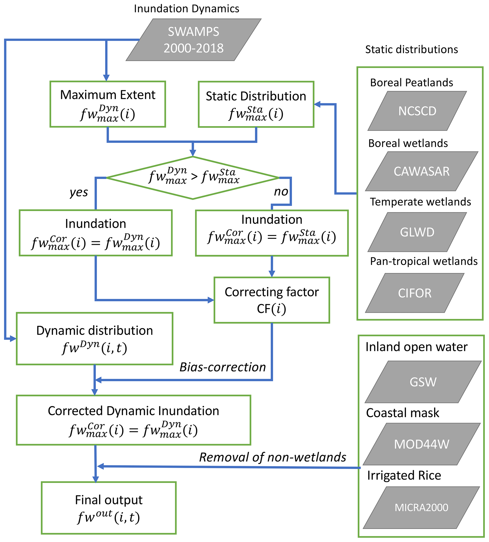
Figure 1 Flow chart of the method describing the wetland extent estimate from SWAMPS and other water body datasets to consolidate our WAD2M product. The chart describes the step calculating fw in each 0.25^∘ grid cell i at time (monthly) t.

We added missing wetlands to SWAMPS by fusing it with the best available maps and inventories of under-represented wetlands separately across three latitudinal bands. For northern wetland inventories, we used the Northern Circumpolar Soil Carbon Database (NCSCD; Hugelius et al., 2013) to map permafrost and non-permafrost peatlands (Histels and Histosols). Mineral soil wetlands were mapped from a SAR-based map by including occurrences of wetlands in the circum-Arctic (Widhalm et al., 2015) outside areas mapped as peatlands by the NCSCD. In the tropics, we used a 231 m resolution pan-tropical dataset based on the geomorphic classification approach (Gumbricht et al., 2017). For temperate regions not covered by either the boreal or tropical datasets, we used the 1 km Global Lakes and Wetlands Database (GLWD) Level 3 after removing Class 1–3 lakes and rivers (Lehner and Döll, 2004). A global dataset of monthly irrigated and rainfed crop areas (MIRCA2000) at a 10 km resolution was used to remove rice agriculture (Portmann et al., 2010). Lakes, ponds, rivers, and other permanent inland water bodies were removed using the Landsat Global Surface Water Explorer (GSW) dataset (Pekel et al., 2016). An ocean–coastline mask based on MOD44W Collection 6 (Carroll et al., 2009), a 250 m resolution annual product from the Moderate Resolution Imaging Spectroradiometer (MODIS) remote sensor, was used to remove ocean waters. The new SWAMPS v3.2 (Jensen and McDonald, 2019) is an updated version of SWAMPS v2.0 (Schroeder et al., 2015) that was used as input in the hybrid wetland product SWAMPS-GLWD (Poulter et al., 2017), the predecessor of WAD2M. The major differences between WAD2M and SWAMPS-GLWD are that (1) WAD2M uses an updated version, SWAMPS v3.2, with improved algorithm and ancillary datasets; (2) WAD2M uses multiple static wetland maps as mergers in the processing (while SWAMPS-GWLD only considers GLWD in the processing); (3) WAD2M includes removal of lakes, ponds, rivers, streams, and irrigated rice paddies; and (4) WAD2M uses a globally consistent ocean–land mask.

To characterize the temporal dynamics, three wetland statistics were computed: (1) mean annual minimum (MA_min), (2) mean annual maximum (MA_max), and (3) long-term annual maximum (MA_Lt). For each 0.25^∘ grid cell, the annual magnitude in wetland area can be calculated as the difference between MA_max and MA_min, while wetland areas that do not flood during the average year (i.e., intermittent wetlands) can be calculated as the difference between MA_Lt and MA_min.

2.2 Datasets

2.2.1 Wetland dynamic dataset

The Surface Water Microwave Product Series v3.2 (SWAMPS) is a dataset of long-term, daily time series of the inundated area fraction derived from microwave remote sensing. The SWAMPS dataset provides estimates of terrestrial surface water dynamics, including for wetlands, rivers, lakes, ponds, reservoirs, rice paddies, and episodically inundated areas. SWAMPS provides estimates of the global inundated area fraction (fw) developed under the NASA Making Earth System Data Records for Use in Research Environments (MEaSUREs) program and is updated monthly. SWAMPS fw estimates are derived from a combination of passive microwave brightness temperature and active microwave radar backscatter from a variety of satellite sensors supplemented with a priori knowledge of land cover based on a static MODIS land cover product (Schroeder et al., 2015). The SWAMPS product includes daily gridded DMSP Special Sensor Microwave/Imager and Special Sensor Microwave Imager/Sounder (SSM/I-SSMIS) Pathfinder brightness temperature observations and active microwave backscatter from the NASA SeaWinds QuikSCAT Level-1B Sigma0 product and Advanced Scatterometer Level-1B (ASCAT) product, with ancillary snow water equivalent, land cover map, and normalized difference vegetation index (NDVI) from the Advanced Very High Resolution Radiometer (AVHRR) and MODIS for delineating snow cover and arid and semiarid areas. SWAMPS v3.2 is an update of v2.0 and includes a new cloud and snow mask, a quality control flag, a new land and ocean mask, freeze–thaw detection, and improved sensor intercalibration. For the purpose of this study, the SWAMPS v3.2 dataset, covering the years 2000 to 2018, was merged into a single monthly mean time series using samples flagged as “Valid Observations”. The sample sizes for the monthly mean range from 14–22 d globally with more measurements during the summer months and fewer measurements during winter months. For SWAMPS v3.2, the coastal zone was first filtered out using a Landsat-based 90 m mask of permanent ocean waters defined by the G3WBM global water body map dataset (Yamazaki et al., 2015) and then filtered using the MODIS MOD44W product to keep it consistent with the processing of the GSW dataset. The SWAMPS v3.2 data were remapped to WGS84 using bilinear interpolation at a 0.25^∘ resolution with values aggregated from daily to monthly means.

2.2.2 Open water and land–ocean masks

The Global Surface Water Explorer (GSW) product is derived from 16 d Landsat thematic mapper imagery at a 30 m spatial resolution and identifies the presence or absence of water bodies over the period 1984–2016 (Pekel et al., 2016). We used this dataset to represent permanent water bodies which we define as those covered by open water for more than 50 % of the months during this time period. We used this as a permanent-water-body mask to avoid including temporary water bodies that are considered wetlands in our working definition. This distribution of long-term maximum permanent water was re-gridded to a 0.25^∘ fractional area per grid cell and used for removing inland-water areas from SWAMPS v3.2. Because the coastal regions were masked out in the processing of SWAMPS, we used the MODIS product MOD44WC6 (Carroll et al., 2009) to generate an ocean mask in the processing of GSW to avoid over-deducting. The coastal region is defined as land areas along the coastline within 4 pixels (∼ 1 km) and was then intersected with the ocean-labeled pixels from MOD44WA1 to separate the ocean from inland water. The resulting ocean mask was then applied to remove coastal wetlands in GSW. The static long-term open-water area excluding coastal regions in GSW is 4.5 Mkm², compared with the river and stream surface areas of 0.8 Mkm² (Allen and Pavelsky, 2018).

2.2.3 Static wetland distributions

We used static wetland maps to fill gaps left by wetland types that are under-represented or missed by the SWAMPS dataset. However, most static maps do not have global coverage or tend to have lower accuracy compared to the regional products, leaving us to take a separate merging approach for each of the three latitudinal bands.

Many arctic wetlands, including peatlands, do not have surface inundation and thus are not captured by SWAMPS 3.2, but they still emit methane. We use the Northern Circumpolar Soil Carbon Database (NCSCD) to map permafrost and non-permafrost peatlands based on the Histel and Histosol soil orders (Hugelius et al., 2013). The NCSCD dataset is a digital polygon-based database compiled from harmonized regional soil classification maps in which data on soil order coverage have been linked to pedon data. In this study, the NCSCD wetland distribution is used as supplementary data for the latitudinal bands from 60–90^∘ N. In this study we use a gridded version with a spatial resolution at 0.25^∘. Permafrost and non-permafrost peatlands (Histels and Histosols, defined as > 40 cm surface peat) are mapped in the NCSCD from harmonized regional and national soil maps (Hugelius et al., 2013). However, these maps do not include occurrences of mineral soil tundra wetlands (with organic soil horizons of 0 to 40 cm) or smaller wetland complexes (Hugelius et al., 2020). To better include these types of wetlands, the NCSCD soil maps were combined with CircumArctic Wetlands based on Advanced Aperture Radar (CAWASAR) by Widhalm et al. (2015). The SAR data identify both organic and mineral wetland soils. They are based on Envisat advanced SAR data acquired in Global Monitoring mode (medium resolution) under frozen soil conditions; this represents surface roughness which can serve as a proxy for wetness levels in tundra. The wettest class was included as wetland. It corresponds to soils with > 25 kg C m² in the top 100 cm (Bartsch et al., 2016). To avoid double counting of organic wetlands (peatlands) the datasets were overlaid so that any overlap between the datasets was removed, maintaining the NCSCD in the output data. The merged static map covers 2.3 Mkm² for the high latitudes (> 60^∘ N), including peatlands and mineral wetlands in the tundra biomes.

The distribution of tropical wetlands, including annually or seasonally waterlogged area and tropical peatlands, are derived from an expert-system mapping product (Gumbricht et al., 2017). We used the Center for International Forestry Research (CIFOR) wetland distribution for adjusting wetlands in the latitudinal bands from 60^∘ S–40^∘ N. This static map was generated by combining satellite images and topographic convergence indices (TCIs) by CIFOR. The TCI indices are calculated based on the Shuttle Radar Topography Mission (SRTM) digital elevation model (DEM) at a 250 m resolution with precipitation climatology from the WorldClim global dataset (Hijmans et al., 2005). A simplified hydrological model was used to estimate the local vertical water balance, runoff, and flood volumes. The topographic and hydrologic data are merged with MODIS (MCD43A4) images used for estimating the duration of wet and inundated soil conditions. The estimated areas of tropical peatlands and wetlands are ∼ 1.7 and ∼ 4.7 Mkm² respectively. The estimated extent of CIFOR for the Cuvette Centrale tropical African peatland in the Congo Basin is 125 400 km², which is in agreement with 145 500 km² of a recent independent field investigation (Dargie et al., 2017).

The Global Lakes and Wetland Database (GLWD) (Lehner and Döll, 2004) is a global database of lakes, reservoirs, and wetlands based on the aggregation of aerial surveys, surveyor maps, and inventories at global and regional scales. While GLWD was generated from data sources now decades old, for some regions, it still represents the most complete wetland database available today. In this study, the GLWD wetland distribution is used to cover the temperate wetland only in the latitudinal band 40–60^∘ N, outside the range of NCSCD and CIFOR. We used the Level-3 product, a global raster map that contains 12 classes of water bodies and wetlands at the 30 s resolution. We excluded the classes representing lakes, rivers, and reservoirs (1–3) and estimated the area of fractional wetland classes (9–12) as the midpoint from the range of each class. We then calculated the total fraction of wetland from all classes in 0.25^∘ pixels. The estimated total wetland extent in GLWD is 8.7 Mkm² for the globe and 2.7 Mkm² for the 40–60^∘ N bands.

2.2.4 Irrigated rice distributions

The distribution of rice paddies is derived from the global dataset of monthly irrigated and rainfed crop areas for the year ca. 2000 (MIRCA2000) (Portmann et al., 2010). The datasets used to develop MIRCA2000 are based on compiling census-based land use datasets downscaled to a grid-cell level and thus are generally consistent with subnational statistics collected by national institutions and by the FAO (Food and Agriculture Organization of the United Nations). For this study, we extracted the annual maximum area of irrigated rice paddies from its original resolution at 5 arcmin and remapped to a 0.25^∘ resolutions. We did not consider rainfed rice as we could not reliably separate lowland from upland cropping practices, with only the latter seasonally contributing to surface inundation. The estimated rice paddies in MIRCA2000 (irrigated 0.64 Mkm², rainfed 1.13 Mkm²) are largely consistent with census-based national and subnational statistics from the FAO (1.54 Mkm² for total area at ca. 2000) and slightly lower than a remote sensing estimate for irrigated rice paddies (0.66 Mkm²) (Salmon et al., 2015). We thus apply the monthly rice cover from 2000 across the entire 2000–2018 time series. This assumption ignoring year-on-year change in rice paddy area is reasonable given that its area increased by < 1.6 % over 2000–2017 according to IRRI world rice statistics (http://ricestat.irri.org:8080/wrsv3/entrypoint.htm, last access: 6 May 2021).

2.3 WAD2M evaluation

WAD2M was evaluated against several, both static and dynamic, independent datasets of wetland area and surface inundation (Table A1). We used a set of satellite-based terrestrial water dynamics to evaluate the trends in temporal patterns of WAD2M, including (1) global soil moisture time series based on the ESA Soil Moisture and Ocean Salinity (SMOS) mission (Level 4; Kerr et al., 2012), (2) a global inundation time series from the Global Inundation Extent from Multi-Satellites (GIEMS version 2) (Prigent et al., 2020), (3) a global land water mass dynamics product from the Gravity Recovery and Climate Experiment (GRACE) mission (Landerer and Swenson, 2012), and (4) a global inundation dynamics from a prognostic run of a land surface model (LPJ) based on a topography-based hydrological model (TOPMODEL) using Climatic Research Unit (CRU) meteorological forcing (Zhang et al., 2018). We also compare WAD2M to a global static map from Tootchi et al. (2019) (regularly flooded wetlands plus groundwater-driven wetlands based on topographic index; hereafter denoted as Tootchi2019) and to regional static maps available over the West Siberian lowlands (Terentieva et al., 2016) and Amazon Basin (Hess et al., 2015). The similarity of WAD2M performance to these independent validation data is evaluated using the kappa index.

3 Results

3.1 Effect of data processing on the results

Globally, WAD2M (MA_max) identifies 3.6 Mkm² more wetlands compared to SWAMPS v3.2 (Table 1). On a continental scale, the wetland extent of SWAMPS v3.2 is in general agreement with inventories except for pronounced discrepancies for tropical wetlands (e.g., Amazon lowlands and tropical Africa), central Asia, and the Sahel regions. The lower area of tropical wetland in SWAMPS v3.2 is generally due to the influence of dense forest canopies. It should be noted that SWAMPS v3.2 detected more wetland area in India than in southeastern China, due to the inclusion of rice paddies in SWAMPS v3.2 that are masked out in WAD2M. Figure 2 shows the comparison of the latitudinal gradient between the original SWAMPS and WAD2M. Generally, WAD2M maintains the same latitudinal pattern as the original SWAMPS, where the peak of wetland area occurs in latitudinal bands of 40–50^∘ N for boreal wetlands and there is another peak around the Equator for tropical wetlands.

Table 1 Three states of inundation (unit 10³ km²) at different steps of the processing of WAD2M.

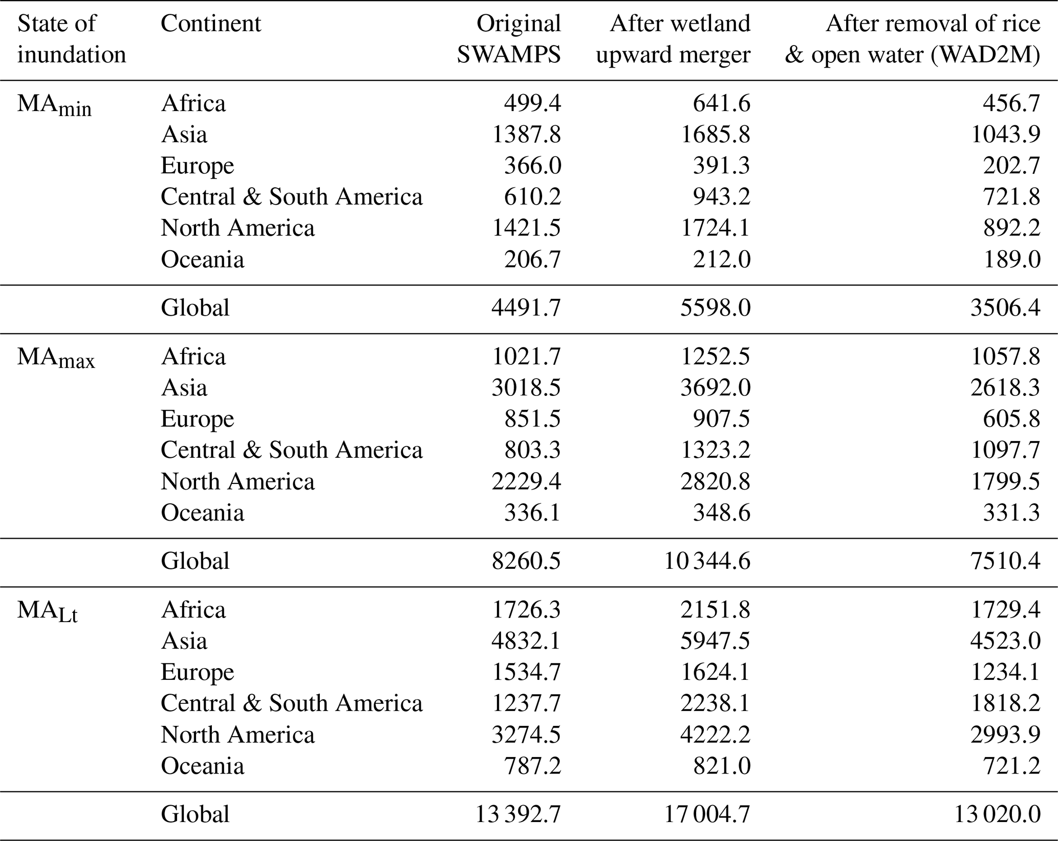
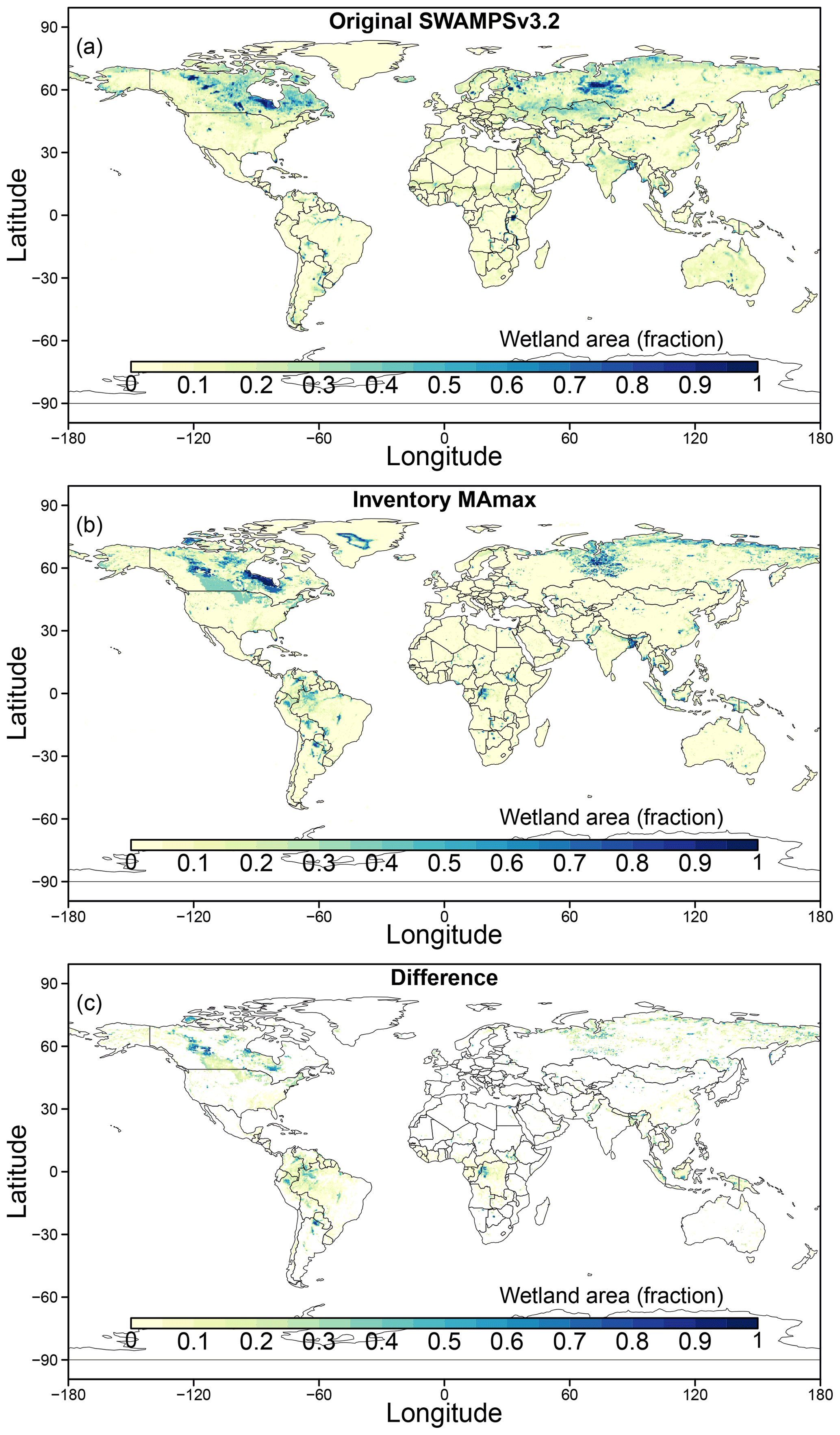
Figure 2 Global maps of wetland fraction before and after processing for (a) global distribution of MA_max of SWAMPS; (b) global distribution of MA_max superimposed by NCSCD, GLWD, and CIFOR; (c) difference in MA_max between inventories and original SWAMPS (inventories minus SWAMPS). Here the positive difference is shown as only the regions with positive values after applying the upward correcting factors.

Table 1 quantifies the effect of the data processing steps on the continental and global estimates of wetland area. The total area including all water bodies such as rice paddies, rivers, streams, lakes, ponds, and reservoirs after fw_max correction is 17.0 Mkm² for MA_Lt. This number is close to the downscaled GIEMS-D15 (17.3 Mkm²), also produced through data merging, suggesting a good agreement between the two products. Applying the fw_max correction leads to a ca. 20 % increase for the three states of inundation relative to SWAMPS v3.2. As intended, the augmentation with inventories filled many missing or underestimated wetland areas of the SWAMPS dataset, which include the Congo floodplain, Amazon Basin lowlands, the Pantanal, Southeast Asia peatlands, and peatlands in high latitudes (i.e., Hudson Bay lowlands and West Siberian lowlands). The highest increase in wetland areas between SWAMPS v2.0 and SWAMPS v3.2 occurs in Asia, followed by North America in the fw_max correction step. However, when we subsequently removed open water and rice paddies in the last step, the increase in wetland area for Asia, North America, and Europe is eliminated. As a result, only South America has a higher wetland area in WAD2M than in SWAMPS v3.2.

3.2 Spatial distributions

3.2.1 Global distributions

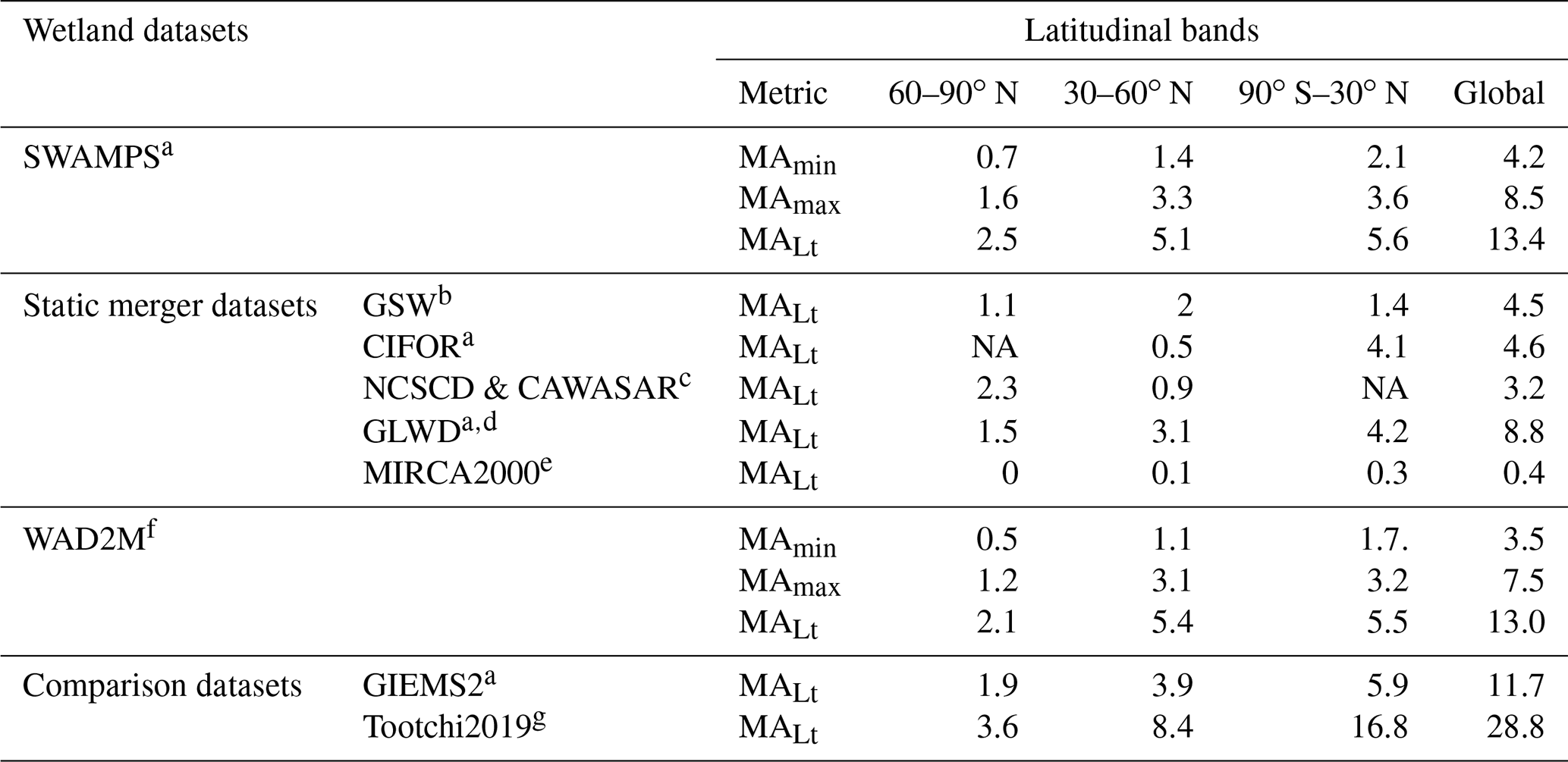
Our estimated total annual maximum area of global vegetated wetlands (excluding Greenland and Antarctica) is ∼ 13.0 Mkm² (Fig. 3a). This estimate consists of 3.5 Mkm² of mean annual minimum wetlands (Fig. 3b), 4.0 Mkm² of seasonally inundated wetlands (MA_max minus MA_min) (Fig. 3c), and 5.5 Mkm² of intermittently inundated wetlands (MA_Lt minus MA_max) (Fig. 3d). Our estimated global total wetland area is slightly higher than that of GIEMS2 (Table 2) but is lower than that of a high-resolution version of the GIEMS initial version GIEMS-D15, which reports a long-term maximum of 17.3 Mkm² (Fluet-Chouinard et al., 2015). Considering that WAD2M conservatively excludes rice paddies (0.59 Mkm²), rivers, streams, and lakes and ponds (2.52 Mkm²) while GIEMS-D15 includes these water bodies, one possible conclusion is that WAD2M applies the upward mergers of CIFOR and NCSCD, which has lower wetland estimates than those of GLWD, causing a lower long-term maximum than in GIEMS-D15. In addition, our estimated total area for intermittently inundated wetlands is close to the 5.2 Mkm² reported for similar wetlands by GIEMS-D15, suggesting a good agreement for temporarily inundated areas between two independently developed products. Other recent studies (Hu et al., 2017; Tootchi et al., 2019), however, have proposed much higher global wetland areas of 27–29 Mkm², which are likely overestimations due to their approaches based on topographic wetness indices that do not take into account the location of surface water tables. This leads to an overestimation of the inundated area with shallow groundwater tables and large inundated areas in, e.g., central Asia and South America that are not matched by other wetland maps.

Table 2 Summary of wetland areas (Mkm²) in WAD2M by latitudinal bands in comparison with the long-term maximum wetlands from merger datasets applied in the WAD2M processing and independent evaluation datasets.

^a Represents inundated area. ^b Represents open water. ^c Represents peatlands and mineral wetlands. ^d GLWD excludes rivers, lakes, and reservoirs; wetland classes interpreted to be in middle range. ^e Represents irrigated rice paddies. ^f Includes both inundated and non-inundated wetlands but excludes artificial inundation and lakes, ponds, and reservoirs. ^g For Tootchi et al. (2019), we use the composite wetland map based on the topography–climate wetness index (CW-TCI) version and exclude lake areas. NA – not available

Figure 3 Maps of wetland extent in WAD2M for (a) long-term maximum (MA_Lt), (b) mean annual minimum (MA_min), (c) mean annual magnitude (MA_max minus MA_min), and (d) intermittent inundated (MA_Lt minus MA_max).

Permanently inundated wetlands are located in well-documented wetland hotspots, including the Hudson Bay lowlands and West Siberian lowlands, where large extents of peat bogs and fens are not represented by SWAMPS v3.2. In tropical regions, key peatland areas along the Amazonian floodplain, in the Cuvette Centrale of the Congo (Dargie et al., 2017), and in the tropical peatlands in Indonesian Papua are all captured by WAD2M. The subtropical and boreal regions are the main contributors to the seasonally inundated wetlands. For the subtropical regions, the seasonal wetlands are largely located in Southeast Asia and the Sahel, where the variation in wetlands is mainly driven by the annual cycle of precipitation in monsoon regions. For the high latitudes, seasonal wetlands are primarily in the transition region from temperate to boreal across both North America and Eurasia. The high seasonality of inundation in these regions was also captured by the surface inundation retrievals of passive microwave observations from the Soil Moisture Active Passive (SMAP) mission (Du et al., 2018).

The latitudinal distribution of wetland area (Fig. 4) suggest that the Northern Hemisphere middle-to-high latitudes (> 45^∘ N) have the highest coverage of wetland area with 45 ± 5 % of the total area of wetlands, followed by the equatorial region (10^∘ S–10^∘ N). A large portion of the intermittent wetlands are found in the northern middle–high latitudes, in regions that also have large areas of seasonal wetlands. The overall latitudinal pattern in WAD2M is similar to that of other estimates except for the Tootchi2019 one, which has the highest wetland area along the latitude gradient. The exception is over the mid-latitudes (20–40^∘ N) where the wetland areas in GLWD are more extensive than that in WAD2M. The wetland areas in the arctic (> 60^∘ N) in WAD2M have a lower wetland extent than in GLWD and NCSCD but higher than in GIEMS2. WAD2M shows a slightly higher wetland extent in the latitudinal band of 10–15^∘ N compared to the other products, which we attribute to the higher intermittent wetlands in Southeast Asia detected by SWAMPS (Fig. 3d). The latitudinal gradient of the wetland area in WAD2M is similar to that of the previous version, SWAMPS-GLWD (Poulter et al., 2017), but with a reduced wetland area in the arctic (> 50^∘ N) and at mid-latitudes (15–45^∘ N), a consequence of the masking out the inland-water areas from GSW. Surface inundation products (GIEMS2 and SWAMPS) have limited observations in the high latitudes due to underestimates of wetland extent for unsaturated peatlands (Bohn et al., 2015) and due to the presence of snow and ice, and they are not reliable points of comparison in high latitudes.

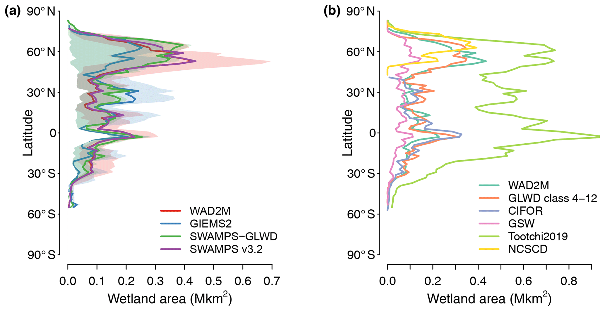
Figure 4 Latitudinal gradient of WAD2M in comparison to existing wetland/inundation products. (a) Comparison with the dynamic inundation products GIEMS2 and SWAMPS-GLWD (previous version of WAD2M). The solid lines represent long-term mean annual maximum (MA_max) with upper (MA_Lt) and lower (MA_min) range of inundated area marked as shaded area. (b) Comparison with static inventory datasets. To make it a fair comparison, lakes, rivers, and reservoirs (i.e., class 1–3 in GLWD) were excluded from GLWD. Lakes (code 4) were excluded from the topographic index (TCI) version of the global wetland composite map from Tootchi et al. (2019) (denoted as Tootchi2019). The wetland area is calculated by a 2^∘ latitudinal band.

3.2.2 Regional comparison

We validated WAD2M against available independent fine-resolution datasets for the two methane-emitting hotspots, Amazon Basin lowlands (defined as the portion of the Amazon watershed below 500 m a.s.l.) and West Siberian lowlands. These two regions represent different wetland subtypes, vegetation compositions, and local hydrology, making them complementary for our validation.

The distribution of wetland area from WAD2M shows a similar spatial pattern for the Amazon Basin lowlands compared to the map based on JERS-1 SAR (Hess et al., 2015), which was used by Pangala et al. (2017) to estimate methane emissions. The distribution of WAD2M has a good similarity (κ= 0.54) to that of the independent, L-band synthetic aperture radar (SAR) map and is slightly lower than that of GIEMS2 (κ= 0.56; Fig. 6a) but higher than all other global products compared (range 0.1–0.2). WAD2M adequately captures the permanently inundated wetlands along with the Amazon Basin river channel network as well as temporarily flooded wetlands during the wet season (Fig. 5a). However, considerable spatial disagreements of the wetland location and extent were found among available datasets when compared with Hess et al. (2015). The disagreements captured in Fig. 6a are primarily related to the seasonally inundated Pantanal floodplains that have relatively flat terrains with dominant herbaceous/shrubland land cover (height < 5 m) and the Pastaza–Marañón wetland basin of the western Amazonia that have large areas of permanently inundated forested swamps with dense-canopy. The WAD2M-estimated wetland fraction exhibits a reasonably good agreement with independent SAR-based wetland products from Hess et al. (2015) for the Pantanal floodplains and the Ucayali–Marañón wetland basin. The WAD2M estimates for Pastaza–Marañón swamps are close to those of CIFOR and Hess et al. (2015) and are considerably lower than those of Tootchi2019. Over the Pantanal floodplains, WAD2M shows moderate-density wetlands, while Tootchi2019 suggest a widespread high-density area over the same extent. The CIFOR estimate is likely an underestimation given the limitations of its topographic-hydrology approach at estimating inundation over flat terrain like the Pantanal.

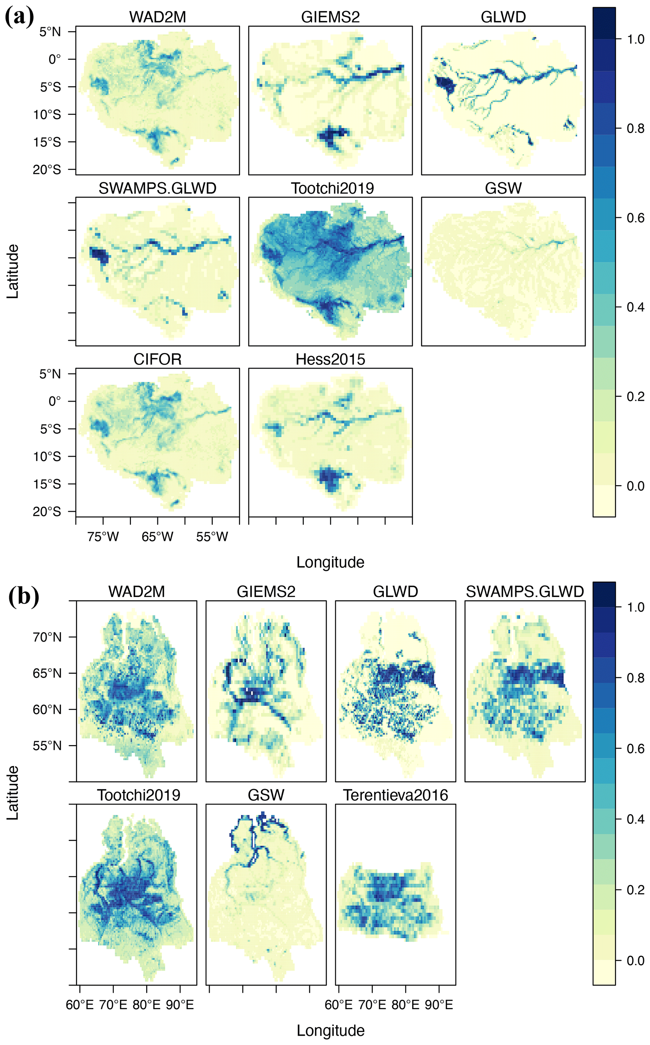
Figure 5 Maps of fractional wetland area from WAD2M in comparison with benchmark datasets for (a) Amazon Basin lowlands and (b) West Siberian lowlands. The wetland maps from WAD2M, GIEMS2, GSW, and CIFOR represent long-term maximum, while the fractional inundation for Amazon lowlands from Hess et al. (2015) represents wetland during the period 1995–1996 for the high-water season. GLWD represents GLWD Level 3 that excludes lakes and reservoirs.

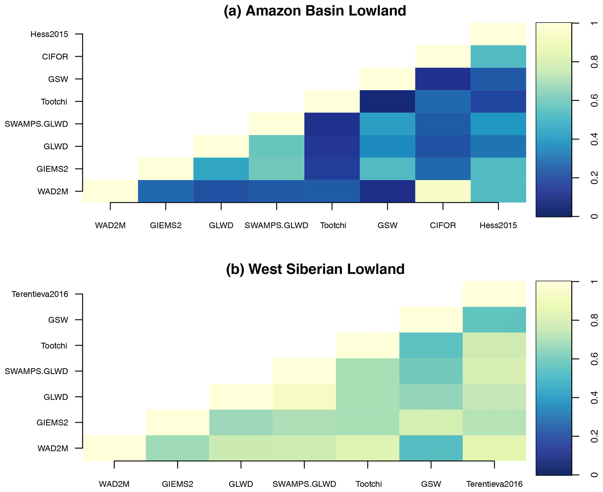
Figure 6 Matrix of kappa coefficient for each pairwise comparison for (a) Amazon Basin lowlands and (b) West Siberian lowlands. The Hess et al. (2015) and Terentieva et al. (2016) data represent two independent regional datasets. All of the datasets in (b) were masked by the map of Terentieva et al. (2016), which is available for the taiga forest zone; hence the calculation of the kappa coefficient excludes the arctic tundra zone (latitude > 65^∘ N).

The comparison of multiple wetland mapping products for the West Siberian lowlands (Fig. 5b) shows that WAD2M permanent wetlands capture the general spatial distribution represented by most other products. WAD2M shows a good agreement with the independent dataset from Terentieva et al. (2016) that combines field survey and satellite images, in particular for inundation peatlands (e.g., fens and bogs) from 55–65^∘ N in the taiga forests. The kappa coefficient of the WAD2M wetland map with Terentieva et al. (2016) for the West Siberian lowlands is 0.70 (Fig. 6b), higher than the value of GIEMS2, GLWD, SWAMPS-GLWD, and Tootchi et al. (2019) (kappa coefficient of 0.18, 0.57, 0.54, and 0.43 respectively). Wetlands in high latitudes above 65^∘ N are more intermittent, caused by thawing of permafrost, and thus related to interannual climate variations.

3.3 Temporal patterns

3.3.1 Seasonal cycle

Distinctive seasonal cycles in WAD2M can be observed across varying latitudinal bands (Fig. 7). The tropics (30^∘ S–30^∘ N) contribute 68 % of the global annual variation in wetland area, owing to the large wetting and drying cycles of tropical wetlands. Despite their large area of intermittent wetlands, the mid-latitudes have a less pronounced seasonal cycle with an average annual minimum of 0.9 Mkm² and average annual maximum of 1.1 Mkm² compared to the tropics and high latitudes. High-latitude wetlands again have a strong seasonal cycle with an average annual minimum of 0.24 Mkm² and average annual maximum of 1.5 Mkm². The seasonal cycle of WAD2M in mid-latitudes is small compared to that of GIEMS2 (Prigent et al., 2020), which is possibly due to different algorithms applied in SWAMPS and GIEMS2, especially in the way the vegetation contribution is accounted for. The seasonal cycle in the high latitudes is highest among the three regions, which is consistent with GIEMS2 and is mainly due to a significant annual freeze–thaw cycle.

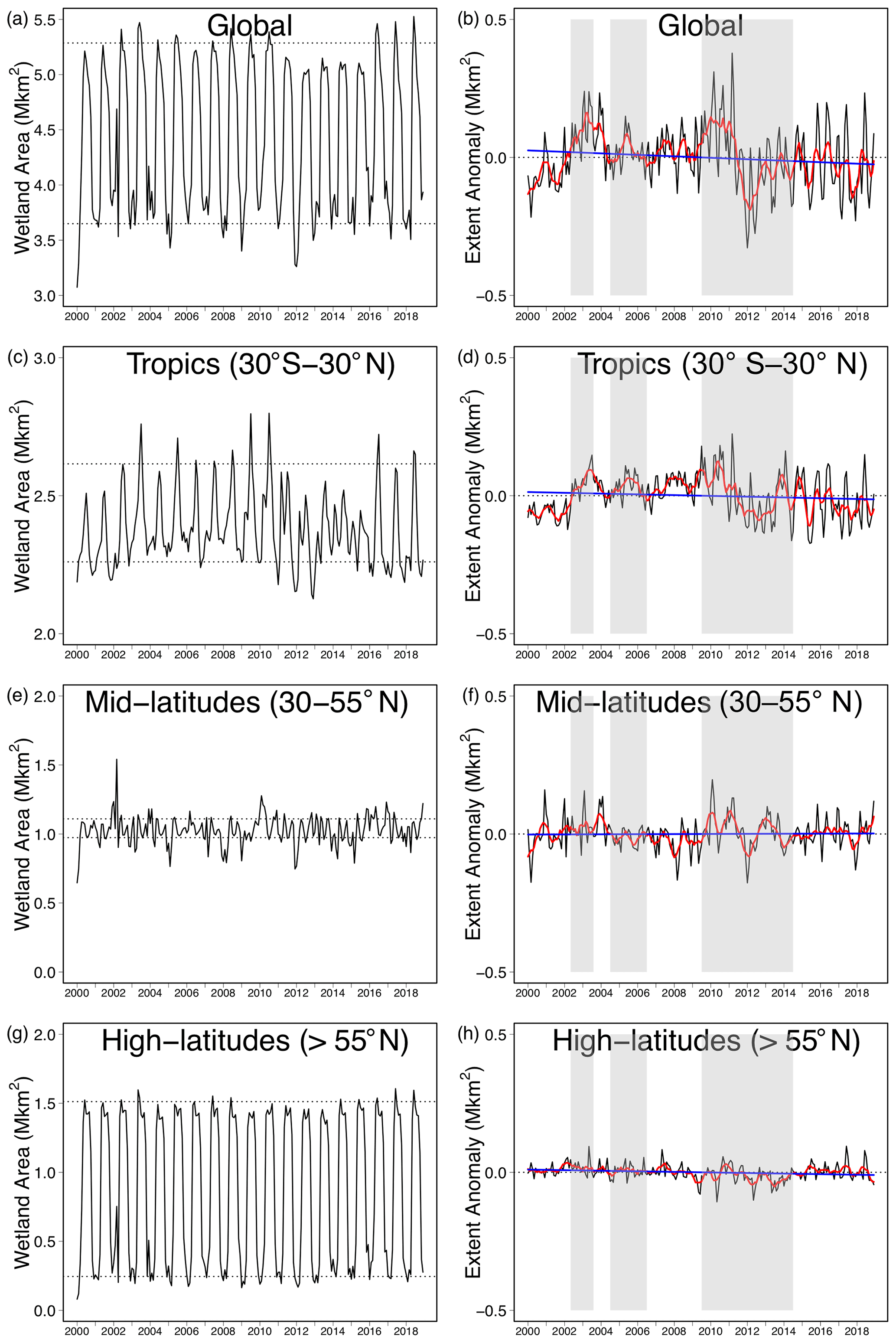
Figure 7 The WAD2M wetland extent and their anomalies from 2000–2018. Monthly mean wetland extent (left column; a, c, e, g) for 2000–2018 in black, for the globe, the tropics (30^∘ S–30^∘ N), and mid-latitudes (30–55^∘ N) and northern high latitudes (latitudes > 55^∘ N). Horizontal dotted lines in the left column panels represent the mean annual maximum and the mean annual minimum. In the right column (b, d, f, h), the deseasonalized anomalies (black) with the 6-month running mean (red) and linearly fitted trends (blue) using least-squares regression are listed. Shaded areas represent the La Niña phase from the NOAA multivariate ENSO index.

Given that there is a surprising scarcity of independent wetland products with which to evaluate the seasonal patterns in middle and high latitudes, we only focus on the comparison of the seasonal cycle for the Amazon Basin, the largest regional contributor to the seasonal cycle of wetland extent. For the Amazon Basin lowlands, the estimates of wetland area exhibit a low seasonal pattern in WAD2M compared to the SAR-based high-resolution estimates from Hess et al. (2015). The flooded/inundated wetlands in WAD2M vary from 0.340 Mkm² in the low-water season (October–November) to 0.401 Mkm² in the high-water season (May–June). The satellite products based on passive microwave bands such as SWAMPS underestimate the seasonality and total wetland areas due to their limited ability to detect inundation outside of large wetlands and river floodplains. This indicates the need to improve the retrieval approach to account for the vegetation contribution in the processing of active and passive microwave signals.

3.3.2 Interannual variation

The interannual variations in WAD2M suggest the effect of climate variations on global wetland extent across varying latitudinal bands (Fig. 7). Monthly anomalies, calculated by subtracting the 19-year mean monthly value from the monthly time series, reveal the changes in global wetlands in response to global climate variability such as El Niño–Southern Oscillation (ENSO) (Fig. 7b). For instance, a strong positive response in wetland areal anomalies was captured by WAD2M during the strong 2010–2011 La Niña event that temporarily increases the terrestrial water storage via affecting precipitation patterns globally (Boening et al., 2012). The signal for the recovery captured by WAD2M, i.e., the decline during the late stage of La Niña, is consistent with the estimated terrestrial water storage from GRACE and the ESA CCI Soil Moisture product (Fig. 8). The linear fit of the pan-tropical wetland anomalies for WAD2M over 2000–2018 shows no significant change (p > 0.1) in the wetland extent for the entire period. There are no trends of wetland extent for mid-latitudes and high latitudes (p > 0.1) as was also found with Landsat imagery (Wulder et al., 2018).

In general, variation in surface water in the tropics is primarily driven by precipitation, and the agreement in the patterns of the surface water extent and precipitation gives confidence in the interannual variability in wetland area estimation. At high latitudes, surface water runoff from snowmelt, not from direct precipitation, contributes towards the lower correlation between inundation extent and precipitation. A strong decline in wetland area during the early stage of El Niño in 2015–2016 was captured by all of the products. The GIEMS2 dataset shows similar patterns to those of WAD2M in two aspects: (1) tropical wetlands contribute to over 50 % of the global total wetland areas and the decadal change in wetland extent is mostly confined to the tropics and (2) the temporal variations in WAD2M are consistent with those of GIEMS2, where a sharp decrease in the tropics was found for 2010–2012, followed by an upward trend from 2013–2014. Note that despite the decline in 2000–2006, the WAD2M estimate is followed by a slight recovery during 2007–2014.

For the interannual variations at a river basin scale (Lehner and Grill, 2013), there is a generally good agreement in the interannual variation in wetland extent between WAD2M and four surface water products that are based on different methodologies (Fig. 8). All the products, including WAD2M, suggest a declining trend in wetland extent in the Amazon Basin since 2012, with strong negative anomalies during 2015–2016 when the strong El Niño event occurred. The temporary increase in wetland extent in WAD2M responding to the strong La Nina event of 2010–2011 is supported by the satellite-based observation of water storage and surface soil moisture, where good agreements of a strong positive phase in terrestrial water were found for the Orinoco Basin and Paraná Basin in South America. The temporal variations in wetland extent for the Ganges, Nile, Yangtze, and Mekong also suggest a good agreement between WAD2M and other products, except for the period since 2015 where GRACE observations suggest a strong decline in the Ganges Basin and Yangtze Basin while WAD2M observations remain constant or slightly decline. This discrepancy could be due to changes in irrigated rice extent, suggesting that the wetland extent in these regions so far is less influenced by groundwater depletion caused by human activity (Rodell et al., 2018). This can be supported by the wetland extent estimate from the TOPMODEL-based prognostic hydrological approach (Zhang et al., 2018), which explicitly excludes influence of human activity and attributes the change to the enhanced tropical precipitation since 2014.

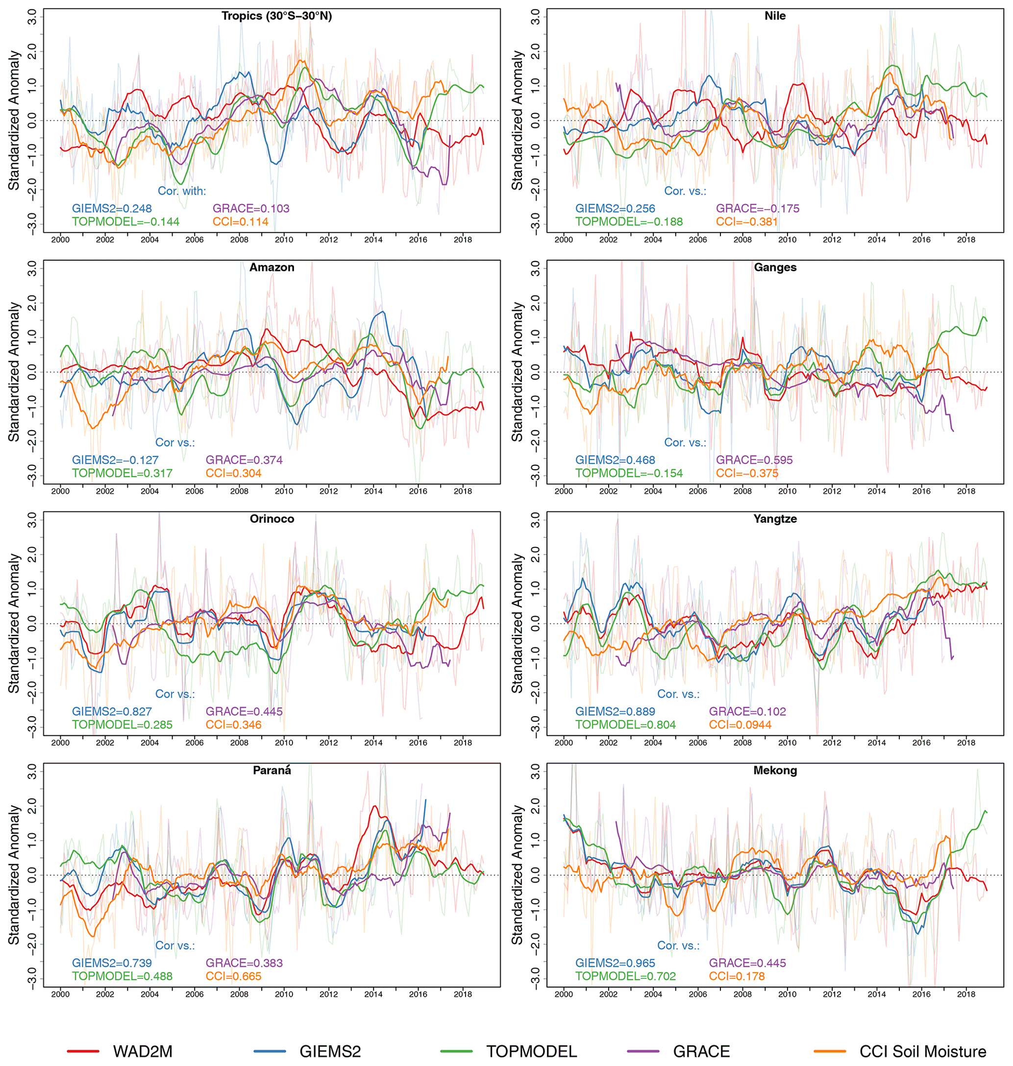
Figure 8 Temporal variations in wetland anomalies in WAD2M in comparison with terrestrial water products from multiple sources. Monthly mean anomaly was calculated as total wetland area within a watershed and was then standardized using a Z score. The shaded lines and the solid lines represent monthly anomalies (standardized value) and trends (12-month running mean of the anomalies). The watershed boundaries are defined using the HydroBASINS dataset (Lehner and Grill, 2013). The correlations in the trend between WAD2M and other sources are listed.

3.4 Uncertainties in wetland areal estimation and future direction

Figure 9 shows the uncertainty range (1σ) of mean annual maximum wetland area across the six global and regional data sources applied in this study. The Amazon Basin lowlands and West Siberian lowlands are two regions with relatively more information compared to the rest of the world (Fig. 9b). There is considerable uncertainty in wetland hotspots such as Hudson Bay lowlands, West Siberian lowlands, and major tropical floodplain regions. The causes of the high uncertainty for the boreal and tropical wetlands differ. Mapping boreal wetlands requires discriminating between wetlands and small ponds, which are both considered wetlands in some inventories (e.g., GLWD) but inland waters in others (e.g., GSW). Thus, the removal of freshwater area is one reason that the boreal wetlands estimates in WAD2M are lower. The uncertainty over tropical floodplain systems is due to the temporal mismatches of the different data sources and to the large seasonal and interannual variability in inundated area. Further, densely vegetated forest canopies in tropical floodplains can lead to systematic underestimation of inundation from satellite-based products. Also, uncertainty in DEMs (from spatial resolution or from whether the measurements are “surface” or “soil”), which serve as the basis of the topographic index that is applied in the hybrid wetland mapping products (e.g., CIFOR; Tootchi et al., 2019), can lead to considerable uncertainty in estimation of wetland extent (Zhang et al., 2016), especially for the vegetated wetlands on complex-terrain surfaces (Su et al., 2015).

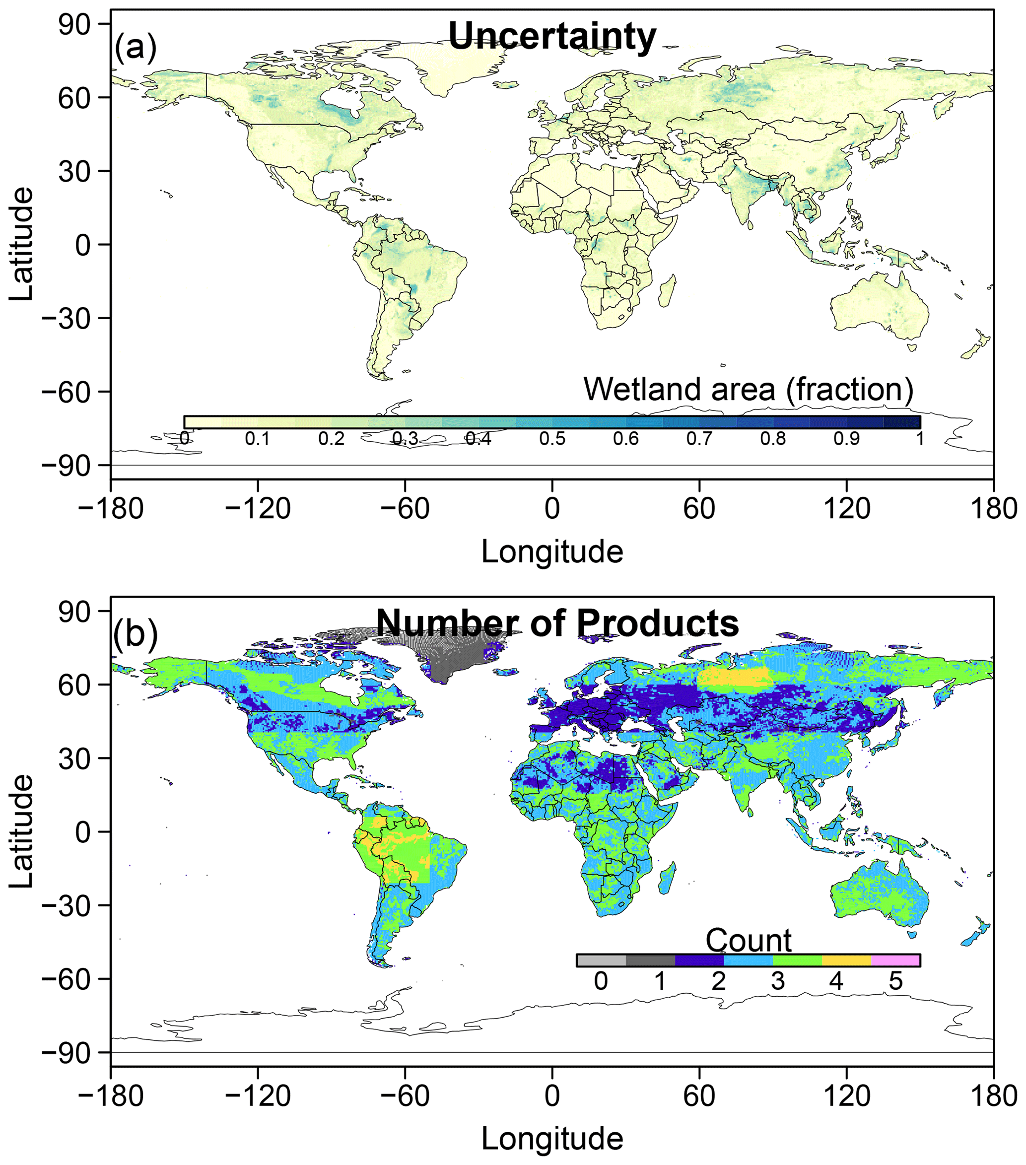
Figure 9 Uncertainty (1σ) of annual maximum wetland area (MA_max) across data sources. The data sources used in the calculation are WAD2M, GIEMS2, GLWD, CIFOR and CAWASAR, NCSCD, Toochi2019, Terentieva et al. (2016), and Hess et al. (2015). (a) Spatial distribution of uncertainty in wetland fraction. (b) Number of products used in the calculation.

4 Discussion

Our study has demonstrated that the spatial distributions of WAD2M based on the data fusion approach show reasonable improvements over existing wetland products and the temporal variations in WAD2M adequately represent interannual variation in response to the climate events such as El Niño–Southern Oscillation. However, the data fusion approach in this study largely relies on the quality of inventories to correct the regions which SWAMPS has limited capacity to detect, which could potentially inflate wetland area in WAD2M when inventories overestimate inundation extent. Due to the scarcity of ground-truth maps for representative regions, further work is needed to confirm the spatiotemporal distribution of inundation captured by WAD2M. In particular, the sensitivity to subcanopy inundation, the a priori knowledge of land cover applied in the retrieval algorithm, and the length of observations can affect the overall accuracy of SWAMPS and thus contribute to the uncertainty in WAD2M. For instance, WAD2M reports a vast inundated area in the Sahel region where validation of the SWAMPS retrieval algorithm is lacking due to sparsity of dynamic ground observations (Jensen and McDonald, 2019). In addition, the retrievals of SWAMPS tend to be affected by the low surface emissivity due to the outcrops of limestone deposits in semiarid and arid regions (Schroeder et al., 2015), which thus potentially causes overestimation in inundation in these regions. Moreover, the decadal trends of WAD2M are influenced by the intercalibration of brightness temperature across different microwave sensors, which could potentially introduce inconsistency between different time periods covered by the measurements. Thus, it is important to be cautious with the interpretation of the long-term trends based on WAD2M. Lastly, because the GSW and MIRCA2000 data sources are aggregated to a 0.25^∘ spatial resolution in the processing of WAD2M, the potential overlapping between these two mergers at a fine spatial resolution is ignored, leading to unintentional double accounting when deducting open water and rice paddies from WAD2M.

Future refinements to WAD2M could come from (1) improvements to revisit spatial resolution, spectral range, and the signal-to-noise ratio of remotely sensed data input and (2) refinements to our fusion methodology to use uncertainties to generate ensemble maps. Several new or upcoming satellite missions may provide improved global wetland dynamics in the future version of WAD2M. The Cyclone Global Navigation Satellite System (CYGNSS) GNSS reflectometry (GNSS-R) (Nghiem et al., 2017) demonstrates its capabilities to detect inundation under different vegetation conditions, which is complementary to inventories for evaluation. The NASA Surface Water and Ocean Topography (SWOT), the Copernicus L-band SAR Radar Observing System for Europe (ROSE-L) (Pierdicca et al., 2019), and NASA-ISRO SAR (NISAR) missions will greatly increase our capacity to monitor the spatiotemporal dynamics of wetlands and floodplains at high spatial resolutions (< 50 m), making them immensely valuable resources in the future work of wetland dynamic mapping such as by WAD2M. Commercial satellites provide even higher spatial resolutions with daily revisits; i.e., the Planet Labs Dove constellation, which is intercalibrated, could go beyond providing static maps and provide time series of wetland data (Cooley et al., 2017).

For the methodology, combining products from different satellite sensors (e.g., optical and microwave) and inventories has been proved to be a feasible way to reduce the bias in the spatial distribution of wetlands and provide reliable estimates for the use of global wetland CH₄ studies. However, the spatial resolution of WAD2M is dictated by the resolution of its input data on the wetland dynamic dataset unless a downscaling methodology is applied. Downscaling can also be used to improve spatial resolution using machine learning approaches (Alemohammad et al., 2018; Kratzert et al., 2018; Wu et al., 2017) or physically based hydrological models (Gumbricht, 2018), together with higher-resolution images (e.g., Landsat, ALOS, ALOS-2) which are better suited to capturing inundation features at fine scales. On the other hand, inventories at the regional and national scales are needed for some relatively under-examined wetlands (e.g., in Africa and Southeast Asia), which will help in reliable validation and evaluation for these regions in future quantitative studies of wetlands. Moreover, even with better sensors in the future, improvements on wetland maps from past and future satellite will be necessary for the backward extension of time series.

5 Data availability

The global wetland dynamic dataset in NetCDF format is publicly available at https://doi.org/10.5281/zenodo.3998454 (Zhang et al., 2020).

6 Conclusions

The development of a global wetland product WAD2M has demonstrated the capability to produce maps of wetlands and inundation that are consistent with independent datasets. Combining temporal dynamics from the coarse-resolution product SWAMPS with complementary products and inventories was shown to be a practical means of tracking variations in global wetland extent over time. WAD2M represents the most reliable representation of global vegetated wetland distribution to date and will be useful to estimate wetland CH₄ flux. WAD2M provides valuable information for a range of applications, ranging from understanding the role of floodplains to carbon modeling and general assessment of global response to climate change.

Appendix A

Table A1 Overview of existing global and regional datasets of open water and wetlands and related proxy datasets.