Shipborne measurements of XCO₂, XCH₄, and XCO above the Pacific Ocean and comparison to CAMS atmospheric analyses and S5P/TROPOMI

Measurements of atmospheric column-averaged dry-air mole fractions of carbon dioxide (XCO₂), methane (XCH₄), and carbon monoxide (XCO) have been collected across the Pacific Ocean during the Measuring Ocean REferences 2 (MORE-2) campaign in June 2019. We deployed a shipborne variant of the EM27/SUN Fourier transform spectrometer (FTS) on board the German R/V Sonne which, during MORE-2, crossed the Pacific Ocean from Vancouver, Canada, to Singapore. Equipped with a specially manufactured fast solar tracker, the FTS operated in direct-sun viewing geometry during the ship cruise reliably delivering solar absorption spectra in the shortwave infrared spectral range (4000 to 11000 cm⁻¹). After filtering and bias correcting the dataset, we report on XCO₂, XCH₄, and XCO measurements for 22 d along a trajectory that largely aligns with 30^∘ N of latitude between 140^∘ W and 120^∘ E of longitude. The dataset has been scaled to the Total Carbon Column Observing Network (TCCON) station in Karlsruhe, Germany, before and after the MORE-2 campaign through side-by-side measurements. The 1σ repeatability of hourly means of XCO₂, XCH₄, and XCO is found to be 0.24 ppm, 1.1 ppb, and 0.75 ppb, respectively. The Copernicus Atmosphere Monitoring Service (CAMS) models gridded concentration fields of the atmospheric composition using assimilated satellite observations, which show excellent agreement of 0.52±0.31 ppm for XCO₂, 0.9±4.1 ppb for XCH₄, and 3.2±3.4 ppb for XCO (mean difference ± SD, standard deviation, of differences for entire record) with our observations. Likewise, we find excellent agreement to within 2.2±6.6 ppb with the XCO observations of the TROPOspheric MOnitoring Instrument (TROPOMI) on the Sentinel-5 Precursor satellite (S5P). The shipborne measurements are accessible at https://doi.org/10.1594/PANGAEA.917240 (Knapp et al., 2020).

1 Introduction

The greenhouse gases carbon dioxide (CO₂) and methane (CH₄) and the air pollutant carbon monoxide (CO) are the target constituents of a range of currently orbiting and planned Earth observing satellite missions (e.g., Kuze et al., 2009; Eldering et al., 2017). The latest addition to the fleet of spaceborne sensors is the Sentinel-5 Precursor (S5P) satellite with its TROPOspheric Monitoring Instrument (TROPOMI) in orbit since October 2017 (Veefkind et al., 2012). TROPOMI retrieves, among other constituents, the column-averaged dry-air mole fractions of CH₄ (XCH₄) and CO (XCO) from spectra of backscattered sunlight in the shortwave-infrared (SWIR) spectral range (Borsdorff et al., 2017, 2019; Hu et al., 2018; de Gouw et al., 2020). In parallel to the expansion of the fleet of greenhouse gas sensors in orbit, the European Centre for Medium Range Weather Forecasts (ECMWF) operates the Copernicus Atmosphere Monitoring Service (CAMS) on behalf of the European Commission. CAMS assimilates satellite measurements of atmospheric composition to forecast the global CO₂, CH₄, and CO concentrations at high spatial and temporal resolution using the Integrated Forecasting System (IFS). During our campaign in June 2019, CAMS assimilated XCO₂ and XCH₄ measurements from the Greenhouse gases Observing SATellite (GOSAT) (Kuze et al., 2009), CH₄ and CO measurements from the Infrared Atmospheric Sounding Interferometer (IASI) (Crevoisier et al., 2009), and CO measurements from the Measurement of Pollution in the Troposphere (MOPITT) (Drummond and Mand, 1996) instrument. The ultimate goal is to monitor the mitigation of anthropogenic greenhouse gas emissions and air pollution from global to regional scales (Massart et al., 2014, 2016; Inness et al., 2015, 2019; Agustí-Panareda et al., 2019; Janssens-Maenhout et al., 2020). Validation of the XCO₂, XCH₄, and XCO satellite data mostly relies on ground-based direct-sun spectroscopic observations conducted by the Total Carbon Column Observing Network (TCCON) (Wunch et al., 2011) supplemented by the emerging Collaborative Carbon Column Observing Network (COCCON) (Frey et al., 2019) that measure the column-averaged dry-air mole fractions with similar column sensitivity to the satellites. Likewise, the CAMS model uses TCCON as an evaluation tool (Agustí-Panareda et al., 2019). Most of the observatories of the TCCON and COCCON are located at continental sites. Thus, validation of the satellites and models over the oceans is limited to a few island and coastal observatories (in particular Ascension, Reunion, Tenerife, Japan, California). For the satellite retrievals, ocean–land biases (e.g., Basu et al., 2013) can occur since the ocean surface is dark, and thus, satellites typically have to resort to glint geometry (e.g., Butz et al., 2013) or retrievals above clouds (e.g., Vidot et al., 2012; Schepers et al., 2016), which impose difficulties different from the typical clear-sky nadir observations above land.

To enable the evaluation of satellites and models over the oceans, Klappenbach et al. (2015) developed a shipborne prototype of the EM27/SUN Fourier transform spectrometer (FTS) (Gisi et al., 2011, 2012) which is the instrument used within the COCCON (Frey et al., 2019). The EM27/SUN has proven to be a reliable instrument for XCO₂ and XCH₄ measurements in various studies ranging from ad hoc networks covering a larger region of interest (Hase et al., 2015b; Chen et al., 2016; Toja-Silva et al., 2017; Viatte et al., 2017; Vogel et al., 2019; Dietrich et al., 2020) to mobile deployments (Butz et al., 2017; Luther et al., 2019) for the quantification of localized CO₂ and CH₄ sources. The latest variant of the EM27/SUN incorporates a second spectral detector channel that enables XCO measurements to be conducted simultaneously with observations of XCO₂ and XCH₄ (Hase et al., 2016). The shipborne observations by Klappenbach et al. (2015) were conducted on board the R/V Polarstern during a cruise from Cape Town, South Africa, to Bremerhaven, Germany, in March and April 2014. These measurements were used for evaluating XCO₂ and XCH₄ observations of the Greenhouse Gases Observing Satellite (GOSAT) and for improving the interhemispheric gradient modeled by the IFS for the CAMS CO₂ and CH₄ analysis and forecasting system (Agusti-Panareda et al., 2017).

Here, we report on the further developments of the shipborne EM27/SUN prototype toward routine use as a validation tool over the open oceans. To demonstrate the performance and robustness of the instrumentation and its suitability for satellite and model validation, we deployed the instrument on the German R/V Sonne during the MORE-2 (Measuring Oceanic REferences 2) campaign which led from Vancouver, Canada, to Singapore between 30 May and 5 July 2019. Figure 1 shows the track of the research vessel over the Pacific Ocean. We report on technical developments (Sect. 2), the data processing chain and data quality assessment (Sect. 3), and comparisons to TROPOMI's XCO measurements and CAMS' analysis fields of XCO₂, XCH₄, and XCO (Sect. 4) over the Pacific Ocean. The data collected are publicly available at https://doi.org/10.1594/PANGAEA.917240 for evaluating other datasets, and the shipborne instrument is recommended for routine deployment on ships.

Figure 1 Track of the R/V Sonne (gray line) during the MORE-2 campaign starting from Vancouver, Canada, on 30 May 2019 and entering port in Singapore on 5 July 2019. The blue dots are the locations of all quality-assured EM27/SUN measurements. The map is provided by Wessel et al. (2019).

2 Instrumentation

The EM27/SUN is a commercially available FTS which was developed in cooperation by Bruker Optics and the Karlsruhe Institute of Technology (KIT) (Gisi et al., 2012). The spectrometer has the dimensions $\mathrm{42}\times \mathrm{27}\times \mathrm{35}$ cm³ and weighs about 25 kg. The EM27/SUN uses a CaF₂ beam splitter and a RockSolid™ pendulum interferometer with two cube corner mirrors. The maximum optical path difference of 1.8 cm supports a spectral resolution of 0.50 cm⁻¹. After the sunlight passed the interferometer, a parabolic off-axis mirror focuses it on an InGaAs photodetector with a spectral range of 5500–11 000 cm⁻¹, further called the SWIR-1 channel. Another mirror decouples about 40 % of the beam on a second spectrally extended InGaAs photodetector covering the spectral range of 4000–5500 cm⁻¹ (Hase et al., 2016), called the SWIR-3 channel. Typical exposure times are on the order of 6 s for a single interferogram. Spectra have been generated from raw DC-coupled interferograms using the preprocessor used by the COCCON network, which has been developed in the framework of the ESA project COCCON-PROCEEDS (Hase et al., 2004; Sha et al., 2019). As suggested by Frey et al. (2015), we use water vapor absorption lines to measure the instrumental line shape (ILS).

The EM27/SUN is mechanically robust, but it would not withstand precipitation or sea spray. For the shipborne variant, we assembled a small container that houses the EM27/SUN FTS with its solar tracker, a laptop, and several ancillary sensors (GPS, pressure, temperature) similar to Heinle and Chen (2018). During the entire MORE-2 campaign, we placed the container outside on the port side of the observation deck of the R/V Sonne, which was the uppermost continuously accessible deck available. We chose this spot to avoid obstruction of the direct light path from the sun to the instrument by ship structures. The container is a white lacquered K470 Zarges aluminum box (IP65 waterproof) with dimensions of $\mathrm{95}\times \mathrm{69}\times \mathrm{48}$ cm³ and mass of 13.4 kg when empty. Figure 2 shows a photograph of the container deployed on the ship. The solar tracker is a modified version of the custom-built setup used by Klappenbach et al. (2015) consisting of a mirror assembly on two perpendicular rotation stages that allow for pointing to any azimuth and elevation position of the sun in the overhead sky. For the ship deployment, we covered the solar tracker with a protective housing that has a fused silica wedged window transmitting the incoming sunlight. The solar tracker housing is positioned on top of the box and attached to the rotation stages moving with the azimuth and elevation rotations. The precision required for the pointing of the solar tracker is 0.05^∘ relative to the center of the sun (Gisi et al., 2011) to keep mole fraction uncertainties due to pointing errors below 0.1 %. Our tracking system satisfied this requirement for 79 % of the measurements for which the sun was within the field of view (FOV) of the solar tracker. We observed the largest pointing deviations when high cirrus clouds were present and when the sun was close to the zenith where the azimuth rotation has a singularity. Our filter criteria reliably remove such observations (see Sect. 3.2).

In addition to the main solar tracker, we mounted a f-theta fisheye lens (Fujinon FE185C057HA-1) with a field of view of $\mathrm{185}{}^{\circ }\times \mathrm{185}{}^{\circ }$ under a protective acrylic glass dome onto the lid of the box. A camera (IDS UI-3280CP-M-GL Rev.2) observes the sky through the fisheye lens and provides the position of the sun with an accuracy better than 2^∘ when the sun is not within the FOV of the solar tracker. The ambient pressure and temperature sensors, as well as the GPS antenna, are mounted on the lid as well. The box is equipped with a Pfannenberg PF 66000 fan for ventilation on one side and an air outlet on the other side to prevent the box from overheating, both of which are covered by protective lids against sea spray and precipitation. During the whole MORE-2 campaign, the box interior temperature never exceeded 40 ^∘C. Inside the box, a Raspberry Pi 3 Model B is the central control unit. It allows for remote access via a network to connect to the laptop controlling the EM27/SUN, an Advantech Ark-2150 embedded PC running the solar tracking software (Klappenbach et al., 2015), and a central storage unit (Synology DS2018). The Raspberry Pi continuously reads the ancillary sensors for the box interior temperature, the ambient pressure and temperature, and the GPS position of the instrument. The electronics runs on 24 V DC provided by an AC C-TEC 2410-10 uninterrupted power supply (UPS). In case of a power cut, the Raspberry Pi securely shuts down all devices within the approximately 60 s backup time of the UPS. The whole container weighs about 80 kg and consumes 190 W via a regular 230 V AC line if the measurement electronics is running at full power. The ventilation consumes an additional 160 W if switched on, which was necessary throughout the campaign.

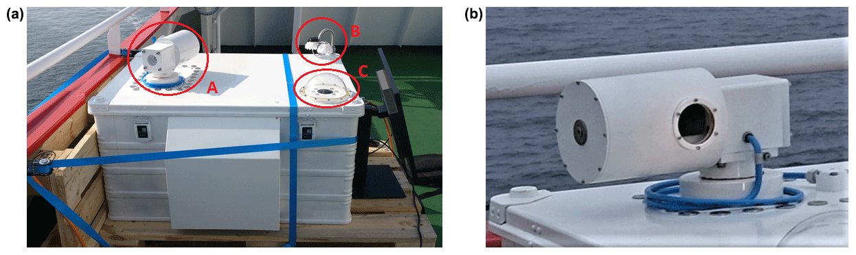
Figure 2 Photograph of the instrument container on board R/V Sonne (a) and the solar tracker housing (b). The solar tracker housing (A in a), the ambient sensors (B in a), and the fisheye camera (C in a) are mounted on top of the box. The solar tracker housing (b) consists of a cylinder which rotates around a horizontal axis in the elevation direction. The cylinder is mounted on a cube which is able to rotate around a vertical axis in the azimuth direction. Sunlight enters the tracker through a fused silica wedged window.

3 Data processing

The quality assessment and the retrievals of XCO₂, XCH₄, and XCO largely follow Klappenbach et al. (2015). Therefore, we summarize the methods here, mostly highlighting the differences and new aspects compared to our precursor study.

3.1 Retrieval of XCO₂, XCH₄, and XCO

The spectral retrieval of the targeted gas concentrations from direct-sun absorption spectra is based on forward modeling of the spectra given a priori concentrations of the molecular absorbers and then iteratively adjusting the concentrations to optimally (in a least squares sense) fit the measured spectra. The spectral retrieval calculates total column number densities of the target gases [GAS] which are a posteriori ratioed by the total column number density of oxygen [O₂] to yield the column-averaged dry-air mole fraction X_GAS of the target gas according to

$$\begin{array}{}\text{(1)}& {\mathrm{X}}_{\mathrm{GAS}}={\displaystyle \frac{\left[\mathrm{GAS}\right]}{\left[{\mathrm{O}}_{\mathrm{2}}\right]}}\cdot \mathrm{0.2094},\end{array}$$

where 0.2094 is the constant column-averaged dry-air mole fraction of molecular oxygen. Referencing the target gas column [GAS] to the oxygen column cancels out instrument- and retrieval-related errors common to both retrievals.

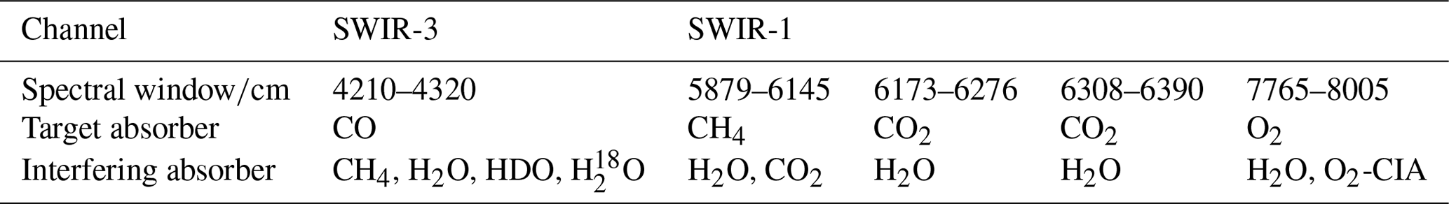
For the spectral retrieval, we use a variant of the RemoTeC algorithm (Butz et al., 2011) which is in use for satellite observation from GOSAT (Butz et al., 2011; Wilzewski et al., 2020), the Orbiting Carbon Observatory (OCO-2) (Wu et al., 2018), and TROPOMI (Hu et al., 2018). We have adapted RemoTeC for transmittance calculations applicable to ground-based direct-sun measurements such as those conducted here. Since the spectral resolution of the EM27/SUN is insufficient to extract profile information from the absorption line shapes, RemoTeC retrieves a scaling parameter on the a priori absorber profiles. The spectral retrieval windows for CO₂, CH₄, and O₂ are located in the SWIR-1 channel and almost identical to the ones used by Klappenbach et al. (2015). The retrieval window for CO is located in the new SWIR-3 channel. Table 1 collects the information on window selection and interfering absorbers. The absorption cross sections of all species are generated from the HITRAN2016 database (Gordon et al., 2017). Meteorological parameters such as pressure and temperature profiles are taken from the National Centres for Environmental Prediction (NCEP) available at NCEP (2000). These NCEP FNL (Final) Operational Model Global Tropospheric Analyses fields are from the Global Data Assimilation System (GDAS) and have a spatial resolution of $\mathrm{1}{}^{\circ }\times \mathrm{1}{}^{\circ }$ and a temporal resolution of 6 h. The a priori profiles for CO₂ and CH₄ are taken from CAMS greenhouse gas analysis (Massart et al., 2014, 2016) and for CO from the near-real-time operational analysis (Inness et al., 2015, 2019). The profiles are interpolated to the time and location of each individual EM27/SUN measurement. CAMS provides CO profiles with 60 model levels on a $\mathrm{0.4}{}^{\circ }\times \mathrm{0.4}{}^{\circ }$ grid and 6 h temporal resolution for the campaign period in June 2019. The CAMS CO₂ and CH₄ profiles have 136 model levels on a $\mathrm{0.25}{}^{\circ }\times \mathrm{0.25}{}^{\circ }$ horizontal grid with 6 h temporal resolution.

Table 1 Spectral windows with target and interfering absorbers. CIA refers to collision-induced absorption.

3.2 Quality filters

The measurements collected during the MORE-2 campaign require quality filtering since cloudy or partially cloudy scenes need to be screened and we want to avoid measurements that are contaminated by the exhaust plume of the ship. To this end, Klappenbach et al. (2015) suggested a cascade of three criteria: a filter based on the DC part of the recorded interferograms, a filter based on the deviation between spectroscopically derived surface pressure and surface pressure measured in situ, and a filter based on the visual identification of steep slopes in the XCO₂ time series.

During the MORE-2 campaign, our FTS recorded the interferograms with the slowly varying DC part included. The DC part is indicative of the overall incoming radiance, and thus, it can be used to track clouds that obstruct the direct-sun view. The DC filter criterion screens measurements either if the DC part I_DC is too small to be direct sunlight or if the fluctuation DC_fluc, defined as

$$\begin{array}{}\text{(2)}& {\text{DC}}_{\text{fluc}}\equiv {\displaystyle \frac{max\left(I_{\text{DC}}\right)}{min\left(I_{\text{DC}}\right)}}-\mathrm{1},\end{array}$$

exceeds 5 %. The DC filter removes 8.39 % of the dataset.

The surface pressure filter compares the surface pressure measured in situ by the ship's meteorological station and the surface pressure calculated from the spectroscopic measurements, as suggested by Wunch et al. (2011). We calculate the spectroscopic pressure from the measured total column number densities of [O₂] and [H₂O] with

$$\begin{array}{}\text{(3)}& {\displaystyle }{p}_{\text{dry}}& {\displaystyle }=\left[{\mathrm{O}}_{\mathrm{2}}\right]\cdot {\displaystyle \frac{M_{{\mathrm{O}}_{\mathrm{2}}}}{N_{\mathrm{A}}\cdot {\mathit{\xi }}_{{\mathrm{O}}_{\mathrm{2}}}}}\cdot g,\text{(4)}& {\displaystyle }{p}_{{\mathrm{H}}_{\mathrm{2}}\mathrm{O}}& {\displaystyle }=\left[{\mathrm{H}}_{\mathrm{2}}\mathrm{O}\right]\cdot {\displaystyle \frac{M_{{\mathrm{H}}_{\mathrm{2}}\mathrm{O}}}{N_{\mathrm{A}}}}\cdot g,\end{array}$$

where M_GAS is the molar mass of the gas molecule, N_A Avogadro's constant, ${\mathit{\xi }}_{{\mathrm{O}}_{\mathrm{2}}}=\mathrm{0.2314}$ (the dry-air mass mixing ratio of oxygen), and g the gravitational constant.

We scale the spectroscopic pressure to the in situ pressure with a factor of 0.9693 such that the ratio

$$\begin{array}{}\text{(5)}& R_{\text{psf}}\equiv \mathrm{0.9693}\cdot {\displaystyle \frac{p_{\text{dry}}+p_{{\mathrm{H}}_{\mathrm{2}}\mathrm{O}}}{p_{\text{in situ}}}}\end{array}$$

scatters around unity within the measurement noise under unperturbed conditions. Any measurement for which R_psf deviates by more than 0.3 % from unity is excluded from further processing, which led to a rejection for 6.2 % of the data.

The third quality filter screens the (rare) situation when our EM27/SUN measurements detected the ship's exhaust plume. During the MORE-2 campaign, this happened in the morning of 8 June 2019 when the ship's exhaust plume crossed the light path. The observations show a steep increase of 2 ppm (parts per million) in XCO₂, while XCH₄ and XCO show no increase. We removed 179 measurements (corresponding to 55 min). After applying all filters, a total of 32 859 (84.38 %) direct-sun measurements pass the filter process and are considered for further processing.

3.3 Bias corrections

After retrieving and quality filtering the XCO₂, XCH₄, and XCO concentrations, the records require bias correction for a spurious dependency on the solar zenith angle (SZA) causing an artificial diurnal cycle (e.g., Wunch et al., 2011) and for species-dependent scaling factors that adjust our spectroscopic measurements to observations of the TCCON whose stations have been compared and scaled to standards of the World Meteorology Organization (WMO; Wunch et al., 2010). We determine the SZA dependency for each species from observations above the Pacific in background air where the columns are expected to be constant and the scaling factors to TCCON via the ratio of side-by-side measurements.

The spurious dependency on SZA causes an underestimation of the column-averaged dry-air mole fractions at high SZAs for each of the target species. Wunch et al. (2011) suggested an empirical correction as a function of SZA Θ according to

$$\begin{array}{}\text{(6)}& {\mathrm{X}}_{\text{corr, GAS}}\left(\mathrm{\Theta }\right)={\displaystyle \frac{{\mathrm{X}}_{\text{GAS}}\left(\mathrm{\Theta }\right)}{{\mathit{\chi }}_{\text{GAS}}\left(\mathrm{\Theta }\right)}},\end{array}$$

where X_{corr, GAS}(Θ) is the corrected column-averaged dry-air mole fraction of the gas under consideration and χ_GAS(Θ) is a third-order polynomial of the form

$$\begin{array}{}\text{(7)}& {\mathit{\chi }}_{\text{GAS}}\left(\mathrm{\Theta }\right)=a{\mathrm{\Theta }}^{\mathrm{3}}+b\mathrm{\Theta }+c,\end{array}$$

with a, b, and c being free fitting parameters. We perform the fit by splitting our time series into morning and afternoon parts at the lowest SZA of the day and consider only those half days which contain a measurement at $\text{SZA}=(\mathrm{45.0}\pm \mathrm{0.5}){}^{\circ }$, which was the case for 26 half days. We reference each measurement to the observation closest to $\text{SZA}=\mathrm{45}{}^{\circ }$, i.e., we choose ${\mathit{\chi }}_{\mathrm{GAS}}\left({\mathrm{45}}^{\circ }\right)=\mathrm{1}$. Furthermore, we identified half days which showed actual atmospheric variability by fitting the SZA dependency in a first attempt and calculating the standard deviation (SD) of the fit residuum. We removed a half day if less than 97 % of its observations were within 2σ of this fit since this indicates actual atmospheric variability which we do not want to misinterpret as spurious SZA dependency. This results in removing 2, 9, and 9 half days from the XCO₂, XCH₄, and XCO records for the fit of the correction polynomial, respectively. Figure 3 shows the corresponding data and the fitted correction polynomials for each target species, and Table 2 lists the parameters defined in Eq. (7) and the coefficients of determination for each fit. The lowest coefficient of determination is found for CO most likely due to the stronger atmospheric variability compared to CO₂ and CH₄.

Table 2 Parameters a, b, and c (and coefficients of determination R²) used for correcting the spurious SZA dependency of the measurements.

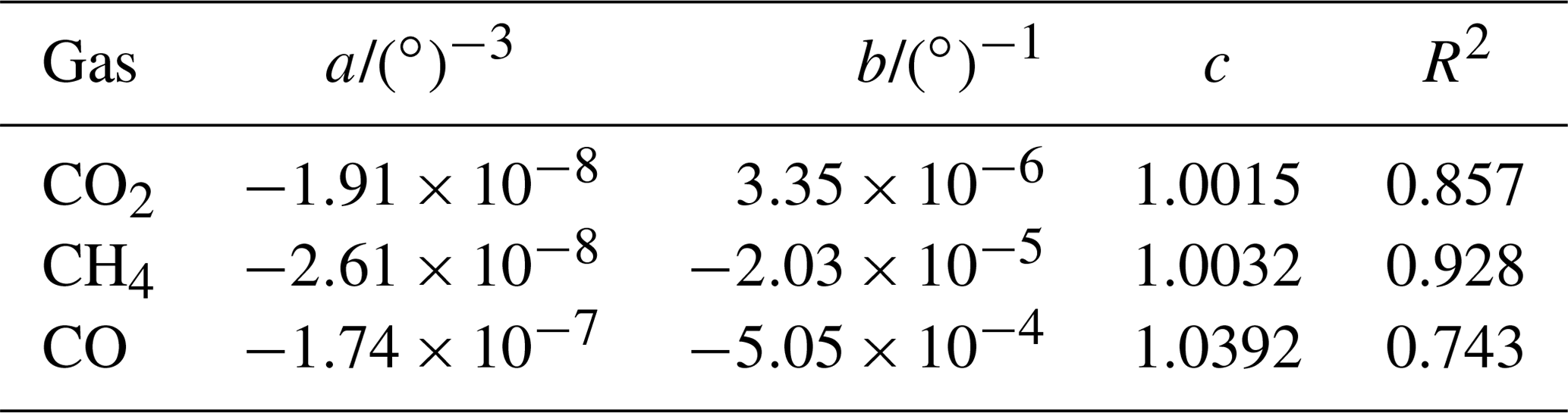
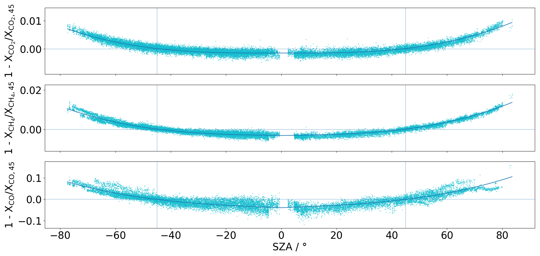
Figure 3 SZA dependency of the retrieved XCO₂ (upper panel), XCH₄ (middle panel), and XCO (lower panel) and the inferred correction polynomial (solid line). Negative SZAs denote morning and positive SZAs afternoon measurements.

After correcting the SZA dependency, we adjust our measurements to those of the TCCON station at KIT, Karlsruhe, to ensure traceability to WMO standards (Hase et al., 2015a). To this end, we performed side-by-side measurements at Karlsruhe for a day before (30 April 2019) and after (23 July 2019) the ship campaign. Figure 4 shows the TCCON measurements alongside the EM27/SUN measurements before and after scaling. Following Klappenbach et al. (2015), we calculate the scaling factor as the mean ratio γ_GAS between the TCCON and the EM27/SUN 1 h means for both days according to

$$\begin{array}{}\text{(8)}& {\mathit{\gamma }}_{\text{GAS}}={〈{\displaystyle \frac{\langle {\text{X}}_{\mathrm{GAS}}^{\mathrm{TCCON}}{\rangle }_{\mathrm{h}}}{\langle {\text{X}}_{\mathrm{GAS}}^{\mathrm{EM}\mathrm{27}}{\rangle }_{\mathrm{h}}}}〉}_{\text{day}}\end{array}$$

for each of the target species. Table 3 lists the scaling factors γ_GAS and their error bars, which we calculate as the standard error σ_γ of the mean using the hourly mean variances ${\mathit{\sigma }}_{\mathit{\gamma },\mathrm{h}}^{\mathrm{2}}$;

$$\begin{array}{}\text{(9)}& {\displaystyle }{\mathit{\sigma }}_{\mathit{\gamma }}=\sqrt{{\displaystyle \frac{{\sum }_{\mathrm{h}}^N{\mathit{\sigma }}_{\mathit{\gamma },\mathrm{h}}^{\mathrm{2}}}{N^{\mathrm{2}}}}},\text{(10)}& {\displaystyle }{\left({\displaystyle \frac{{\mathit{\sigma }}_{\mathit{\gamma },\mathrm{h}}}{{\mathit{\gamma }}_{\mathrm{h}}}}\right)}^{\mathrm{2}}={\left({\displaystyle \frac{\mathit{\sigma }\left(\langle {\text{X}}_{\mathrm{GAS}}^{\mathrm{TCCON}}{\rangle }_{\mathrm{h}}\right)}{\langle {\text{X}}_{\mathrm{GAS}}^{\mathrm{TCCON}}{\rangle }_{\mathrm{h}}}}\right)}^{\mathrm{2}}+{\left({\displaystyle \frac{\mathit{\sigma }\left(\langle {\text{X}}_{\mathrm{GAS}}^{\mathrm{EM}\mathrm{27}}{\rangle }_{\mathrm{h}}\right)}{\langle {\text{X}}_{\mathrm{GAS}}^{\mathrm{EM}\mathrm{27}}{\rangle }_{\mathrm{h}}}}\right)}^{\mathrm{2}},\end{array}$$

where σ() is the SD of the hourly mean and N the total number of hours of side-by-side observations. For CO₂, the scaling factors are consistent within the error bars, and for CH₄, the scaling factors before and after the campaign are consistent at roughly 3 ‰, though the differences are larger than the combined error bars. For CO, the scaling factors before and after the campaign differ by roughly 2 %, which is substantially more than the error bars. We identify a change in the ILS as the most likely candidate for this difference in the scaling factors. The ILS was measured under laboratory conditions before and after the campaign. We also performed ILS measurements at the beginning of the campaign on 2 June 2019, yet it was impossible to assure laboratory conditions there since the measurements were conducted on deck. The pre-campaign ILS differs from the one taken on board the R/V Sonne most likely due to rough handling during the transport from Germany to Vancouver and, in consequence, a slight change in the optical alignment. We could not detect any change in the ILS after shipment back to Germany from Singapore. Thus, we adjust our measurements with the factors derived from the TCCON side-by-side measurements on 23 July 2019. Even after applying the scaling factor, Fig. 4 shows that there is some residual differences between the EM27/SUN and TCCON data growing towards the afternoon. At present, the origin of these differences is unclear. Zhou et al. (2019) suggest further investigations of the TCCON XCO scaling factor based on comparisons of the TCCON to the Network for the Detection of Atmospheric Composition Change (NDACC) and AirCore measurements. Should the TCCON scaling factor be updated in the future, our XCO data will be scaled accordingly.

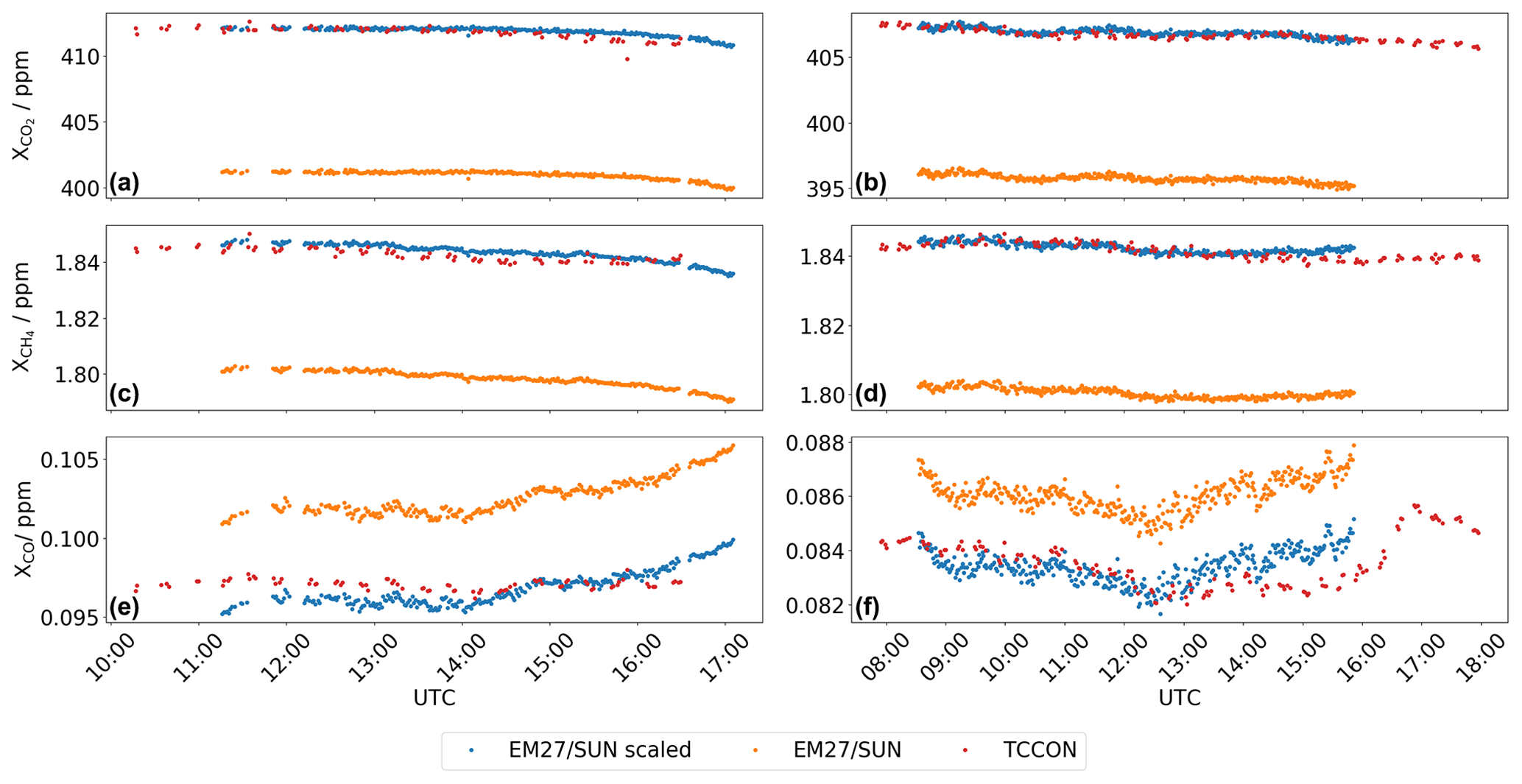
Figure 4 Side-by-side measurements of XCO₂ (a, b), XCH₄ (c, d), and XCO (e, f) by the shipborne EM27/SUN and the TCCON station at Karlsruhe on 30 April 2019 (a, c, e) and 7 July 2019 (b, d, f). EM27/SUN measurements before and after scaling are shown in orange and blue, and TCCON records are shown in red.

Table 3 Scaling factors γ for EM27/SUN XCO₂, XCH₄, and XCO observations as derived from the side-by-side measurements at the TCCON station Karlsruhe (Eq. 8). The uncertainty is the standard error of the mean of the hourly data (Eq. 9).

4 Comparison to TROPOMI and CAMS

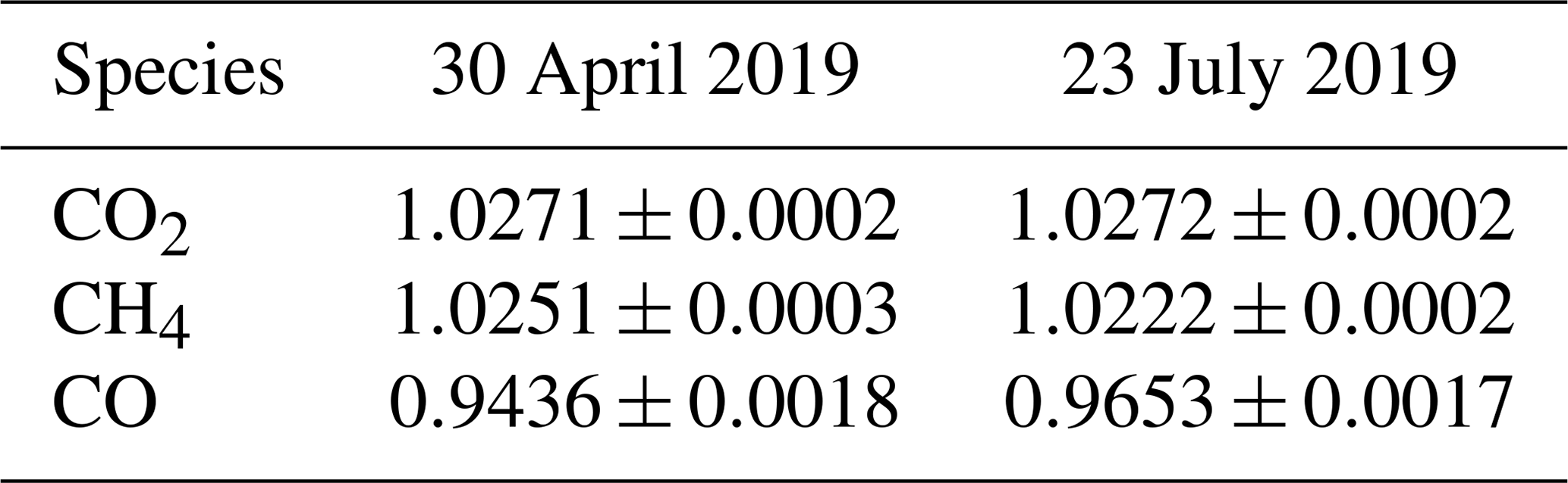
Figure 5 shows the quality-filtered and bias-corrected XCO₂, XCH₄, and XCO records for our cruise over the Pacific Ocean. The trajectory largely follows 30^∘ N of latitude between 140^∘ W and 120^∘ E of longitude, crossing the date line on 14 June 2019. For statistical analysis, we calculate hourly means of our records and use the campaign averaged SD of the hourly means as a measure for our precision, which amounts to 0.24 ppm (0.06 %), 1.1 ppb (0.06 %; parts per billion), and 0.75 ppb (1.03 %) for XCO₂, XCH₄, and XCO, respectively. The data records clearly show that we sampled background air masses for most of the time. We calculate a campaign mean and SD throughout the longitudinal section for each species, finding means and SDs as little as 411.6±0.6 ppm for XCO₂, 1835±7 ppb for XCH₄, and 71±5 ppb for XCO.

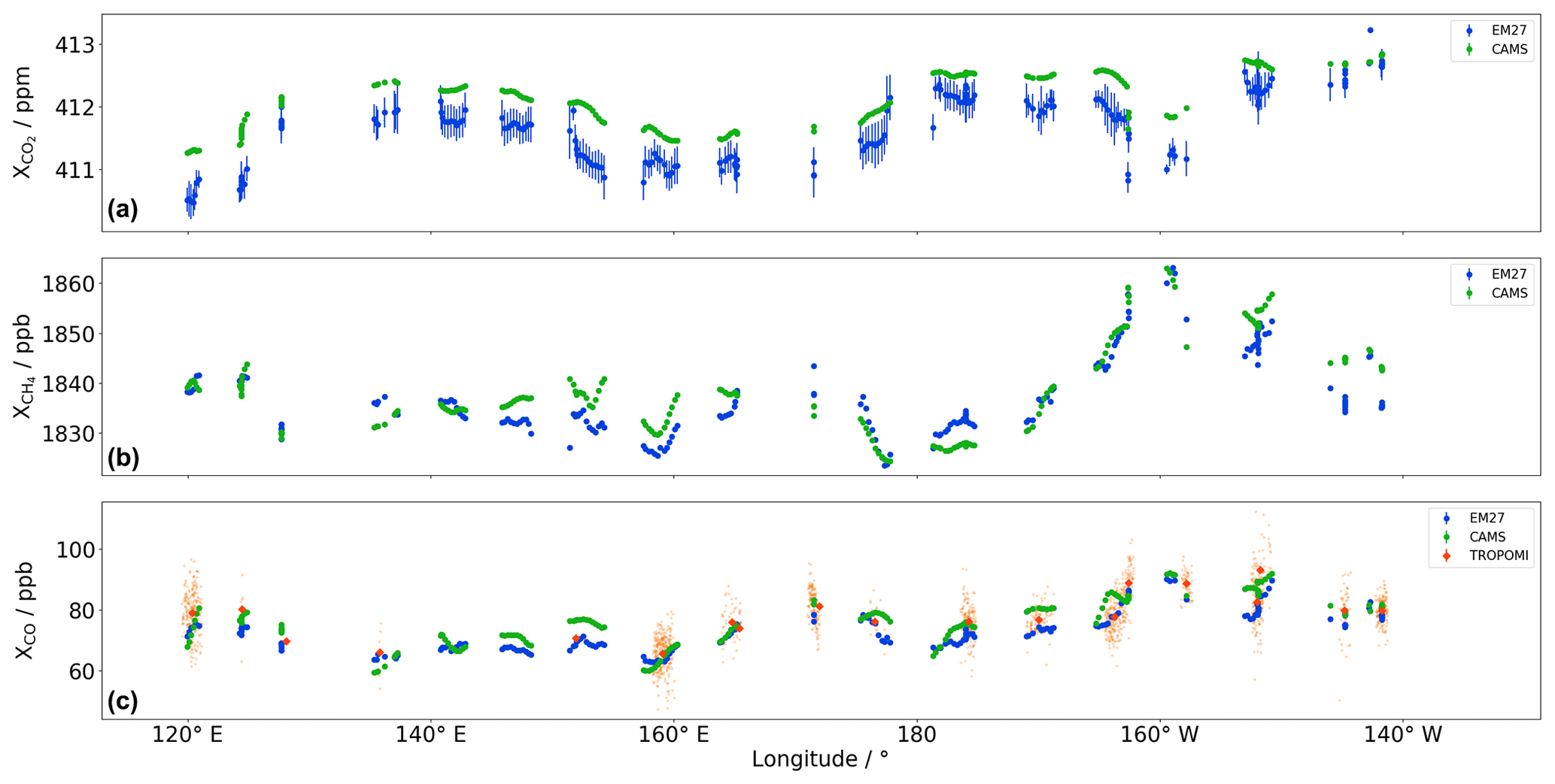
Figure 5 XCO₂ (a), XCH₄ (b), and XCO (c) measured by the shipborne EM27/SUN (blue) above the Pacific alongside coincident CAMS atmospheric composition analysis data (green) and coincident XCO satellite observations by TROPOMI (orange). EM27/SUN measurements and CAMS data are hourly averages, while TROPOMI observations are averaged per overflight. Single TROPOMI measurements are marked small in the background.

Figure 5 compares our observations to column-averaged dry-air mole fractions we calculated from vertical profiles of the CAMS atmospheric composition analyses. These profiles are the same as those we use as a priori for our retrieval. Therefore, the differences between our retrievals and CAMS have no contribution from the a priori profiles being different from CAMS. Furthermore, Fig. 5 shows TROPOMI XCO observations for which we apply coincidence criteria of 0.5^∘ radius and 4 h time span. The TROPOMI XCO data are available at ESA (2018) and have been retrieved by the SICOR algorithm (Landgraf et al., 2016) which allows for retrievals above clouds. The latter capability is important over the ocean since the ocean is dark implying large noise unless the ocean-glint spot is observed or clouds offer a bright reflection target. After filtering with TROPOMI's quality flag (i.e., the internal quality descriptor bounded by 0 and 1 must be larger than 0.5), we find 1783 coincident TROPOMI XCO measurements distributed among 19 d. Although TROPOMI has XCH₄ measurement capabilities, we do not discuss these here since there is currently no ocean data available. Likewise, we do not show any OCO-2 or GOSAT data since the number of coincidences was 43 and 9, respectively, and limited to individual days, which we consider too few for a robust statistical analysis. The SICOR algorithm uses the global chemistry transport model TM5 (Krol et al., 2005) as an a priori source, which introduces a difference in the comparison to our EM27/SUN CO measurements with a priori profiles from CAMS (Borsdorff et al., 2014). We calculate the difference due to the a priori profiles for each EM27/SUN observation and find it to be 0.11±0.40 ppb (campaign mean ± SD) with a maximum of 0.92 ppb. This contribution is small but not entirely negligible compared to the differences we find between our data and TROPOMI CO.

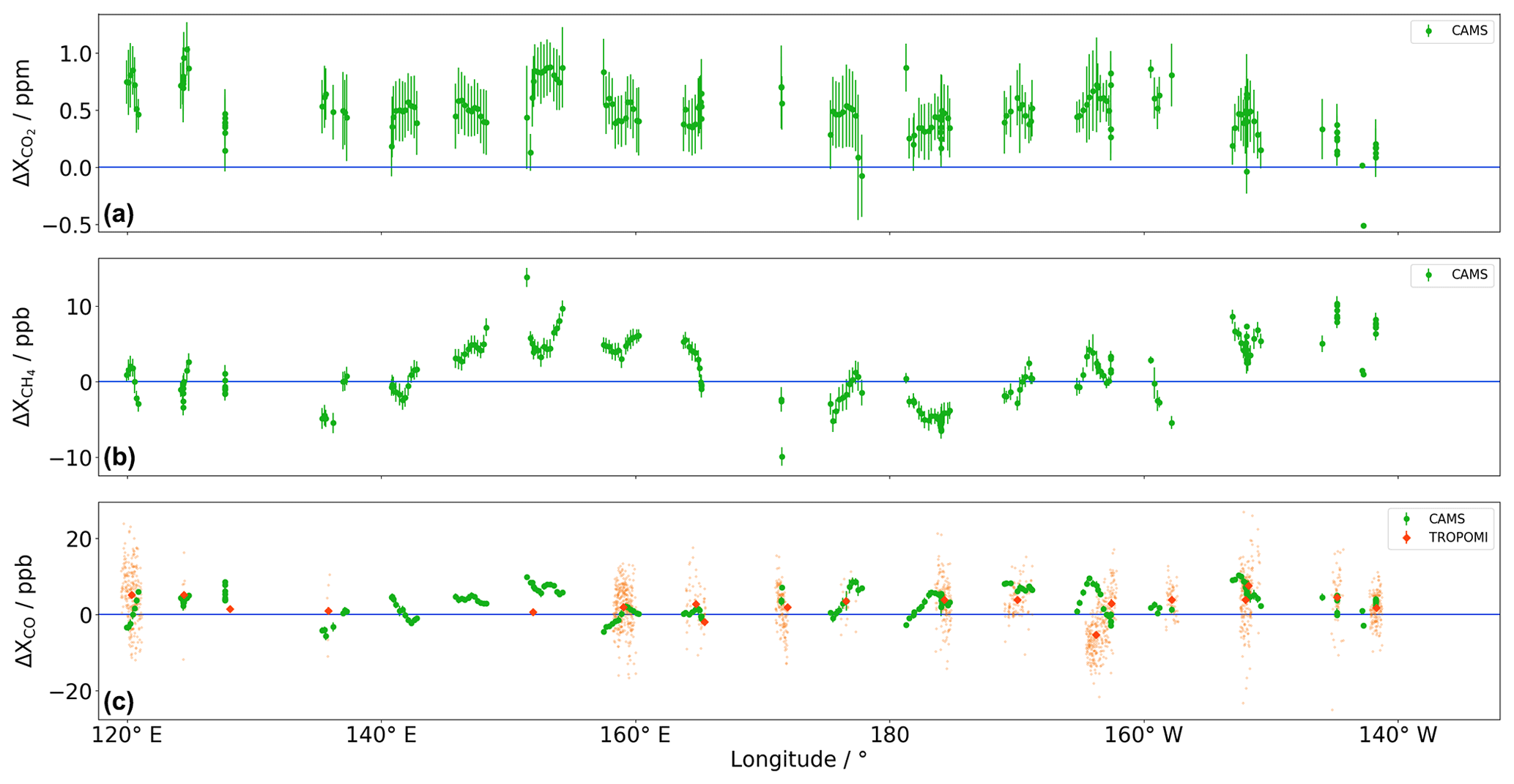
Figure 6 Differences between CAMS and our shipborne EM27/SUN (green) for XCO₂ (a), XCH₄ (b), and XCO (c) and between TROPOMI XCO and our EM27/SUN (orange). The EM27/SUN measurements were subtracted from the CAMS data and coincident TROPOMI observations.

Figure 6 depicts the differences between CAMS and our data and between TROPOMI and our data. We average the differences to CAMS over the entire campaign and calculate the standard deviations of the differences, which amount to 0.52±0.31 ppm for XCO₂, 0.9±4.1 ppb for XCH₄, and 3.2±3.4 ppb for XCO (see also Table 4). Thus, CAMS shows excellent agreement with the shipborne measurements within 1σ for CH₄ and CO and 2σ for CO₂. Maximum differences between the hourly means of CAMS and EM27/SUN observations amount to 1.0±0.2 ppm XCO₂, 13.8±1.3 ppb XCH₄, and 10.3±0.5 ppb XCO, in which the range is the propagated error using the SDs of the hourly mean values. For XCH₄, CAMS tentatively shows an underestimation by a few parts per billion around the date line and an overestimation around 160^∘ E. Further, the intra-day variability of XCH₄ shows a systematic difference on the order of a few parts per billion. However, there is no consistent intra-day pattern that fits all the campaign days. Likewise for XCO, there is an intra-day residual pattern on the order of a few parts per billion but no consistency that informs us of potential model errors or shortcomings of the shipborne measurements.

Table 4 Comparison of the EM27/SUN observations to CAMS model data and coincident TROPOMI XCO measurements. The data indicate the mean differences ± the SD of the differences for the entire record.

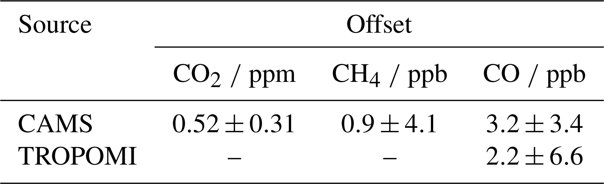
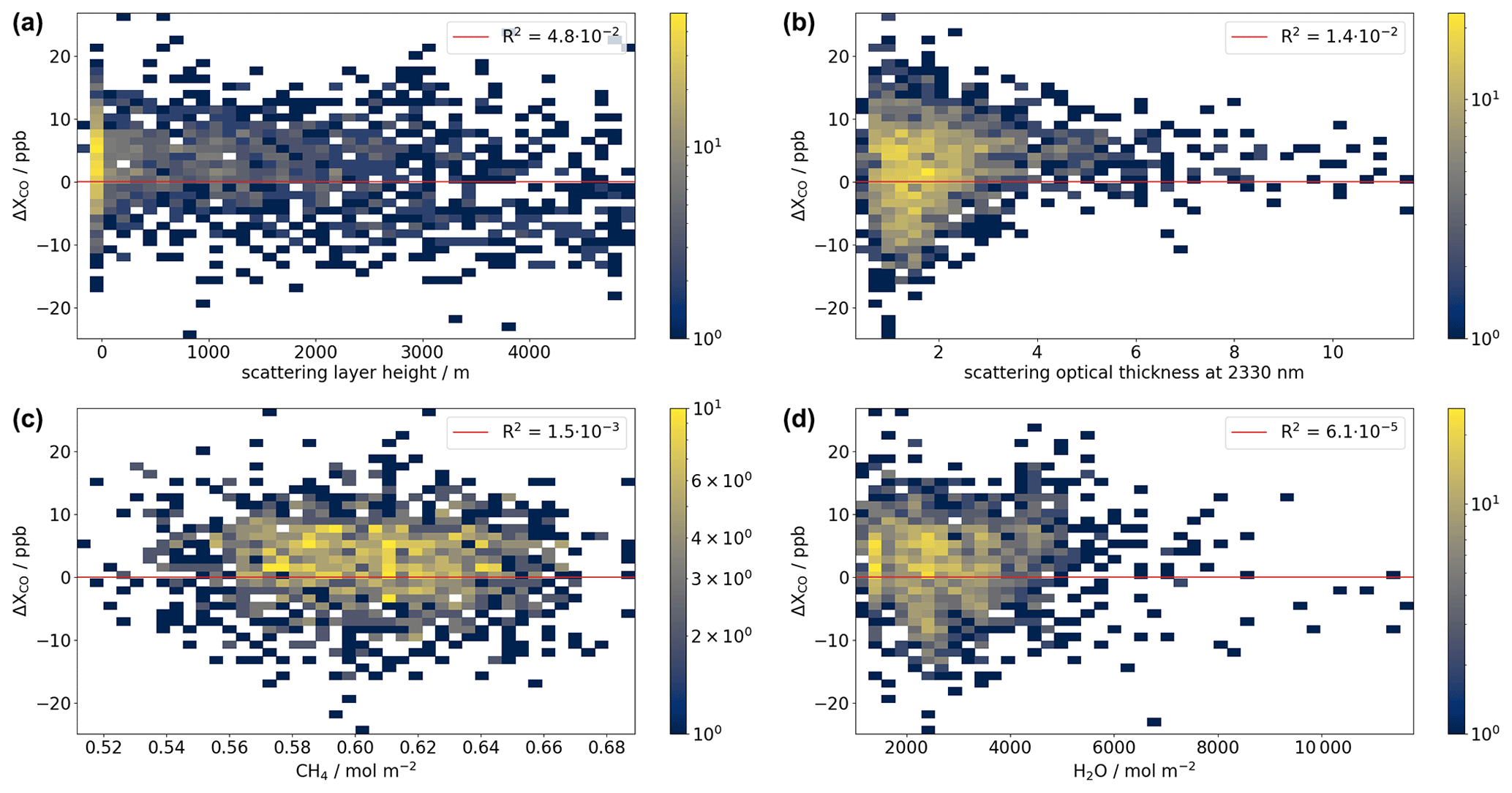
Figure 7 Absolute differences between TROPOMI XCO observations and our EM27/SUN measurements plotted as a function of the SICOR/TROPOMI retrieval parameters scattering layer height (a), scattering optical thickness (b), interfering CH₄ (c, from weak two-band total column), and interfering H₂O (d). The color code indicates (logarithmic) occurrence, and the red line is a linear fit with its coefficient of determination R² given in the upper right of each plot.

TROPOMI XCO also shows very good agreement with our data. The mean difference and standard deviation among the entire campaign record is 2.2±6.6 ppb without any systematic pattern correlating with the position in the Pacific Ocean. Borsdorff et al. (2019) improved the SICOR/TROPOMI CO data product in comparison to TCCON observations by adjusting the spectroscopic database, decreasing the global mean bias below 1 ppb compared to TCCON station records with an SD of 2.6 ppb and a TCCON station-to-station bias variation of 1.8 ppb. We investigated whether the small residual differences correlate with the cloud parameters or interfering absorber abundances that SICOR/TROPOMI retrieves simultaneously with XCO. Figure 7 shows the correlations of the differences with the layer height and the scattering optical thickness of the cloud layer, as well as the atmospheric methane and water column retrieved by SICOR/TROPOMI. Landgraf et al. (2016) find a retrieval bias in the case of CO enhancements in combination with clouds, which we can not assess from our background concentration observations. Furthermore, we find no correlation of the XCO differences with the atmospheric methane and water vapor columns retrieved by SICOR/TROPOMI. These two species show spectroscopic interferences with the CO absorption lines in the SWIR-3 band, and thus, they could be candidates for inducing retrieval errors. Overall, our evaluation suggests that SICOR/TROPOMI provides robust results over clouds and for ocean-glint observations.

5 Data availability

The XCO₂, XCH₄, and XCO records are available for download on PANGAEA at https://doi.org/10.1594/PANGAEA.917240 (Knapp et al., 2020). The CAMS CO₂ and CH₄ data used in the paper is the official CAMS GHG analysis (https://doi.org/10.24380/654b-gm83, CAMS, 2020). The data for CO₂ and CH₄ is available via request to Copernicus Service Desk by emailing to copernicus-support@ecmwf.int or via the CAMS enquiry portal in https://atmosphere.copernicus.eu/help-and-support (last access: 29 January 2020). The CO data is from the CAMS NRT analysis available for download at https://doi.org/10.24380/hhra-8c27 (CAMS, 2019).

6 Conclusions

We deployed an EM27/SUN FTS on board the German R/V Sonne on the MORE-2 campaign cruise from Vancouver to Singapore leaving port on 30 May 2019 and arriving on 5 July 2019. Compared to our precursor study (Klappenbach et al., 2015), our instrument setup was able to withstand environmental conditions, and it ran largely without requiring on-site operating personnel. Plus, the sun-viewing FTS was augmented by another detector to collect solar absorption spectra of CO in addition to CO₂ and CH₄ (Hase et al., 2016). We provide records of the column-averaged dry-air mole fractions XCO₂, XCH₄, and XCO for 22 d of measurements on the Pacific Ocean largely following 30^∘ N of latitude. Our observations are representative of global background conditions; thus, they are useful for assessing the performance of atmospheric models and satellite measurements without perturbations due to local atmospheric variability, and they add to the largely land-based validation data provided by the TCCON and the COCCON. Our measurements show an overall precision (hourly SDs averaged for the whole campaign) of 0.24 ppm for CO₂, 1.1 ppb for CH₄, and 0.75 ppb for CO. Systematic errors due to residual pointing uncertainties, sampling of the ship's exhaust plume, and a spurious dependency on the SZA are treated by filtering flawed data and by empirical corrections. We made our observations compatible with the TCCON through side-by-side measurements before and after the campaign at the TCCON station Karlsruhe. Through comparisons to our data, we evaluate the performance of the CAMS model for XCO₂, XCH₄, and XCO and the performance of XCO measurements by the TROPOMI instrument on board the Sentinel-5 Precursor satellite. Averaged over the entire campaign, the differences to CAMS amount to 0.52±0.31 ppm for XCO₂, 0.9±4.1 ppb for XCH₄, and 3.2±3.4 ppb for XCO. Furthermore, we find the TROPOMI XCO of 2.2±6.6 ppb to be in excellent agreement with the ground-based observations. The instrument is a valuable asset for the validation of satellite observations over sea. In the future, we plan to fully automate our instrument design for routine deployment on ships to enrich validation opportunities over the open oceans where other opportunities are sparse.