the Creative Commons Attribution 4.0 License.
the Creative Commons Attribution 4.0 License.
 | 01 Apr 2021
Feasibility of reconstructing the summer basin-scale sea surface partial pressure of carbon dioxide from sparse in situ observations over the South China Sea
Yao Chen
Yan Bai
Huan Qin
Zhixuan Wang
Baoshan Chen
Xianghui Guo
Minhan Dai
Sea surface partial pressure of CO2 (pCO2) data with a high spatiotemporal resolution are important in studying the global carbon cycle and assessing the oceanic carbon uptake. However, the observed sea surface pCO2 data are usually limited in spatial and temporal coverage, especially in marginal seas. This study provides an approach to reconstruct the complete sea surface pCO2 field in the South China Sea (SCS) with a grid resolution of over the period of 2000–2017 using both remote-sensing-derived pCO2 and observed underway pCO2, among which the gridded underway pCO2 data in 2004, 2005, and 2006 are presented for the first time. Empirical orthogonal functions (EOFs) were computed from the remote-sensing-derived pCO2. Then, a multilinear regression was applied to the observed pCO2 as the response variable with the EOFs as the explanatory variables. EOF1 explains the general spatial pattern of pCO2 in the SCS. EOF2 shows the pattern influenced by the Pearl River plume on the northern shelf and slope. EOF3 is consistent with the pattern influenced by coastal upwelling along the northern coast of the SCS. When pCO2 observations cover a sufficiently large area, the reconstructed fields successfully display a pattern of relatively high pCO2 in the mid and southern basin. The rate of sea surface pCO2 increase in the SCS is 2.4±0.8 µatm yr−1 based on the spatial average of the reconstructed pCO2 over the period of 2000–2017. This is consistent with the temporal trends at Station SEATS (SouthEast Asia Time-series Study; 18∘ N, 116∘ E) in the northern basin of the SCS and at Station ALOHA (A Long-Term Oligotrophic Habitat Assessment; N, 158∘ W) in the North Pacific. We validated our reconstruction with a leave-one-out cross-validation approach, which yields the root-mean-square error (RMSE) in the range of 2.4–5.2 µatm, smaller than the spatial standard deviation of our reconstructed data and much smaller than the spatial standard deviation of the observed underway data. The RMSE between the reconstructed summer pCO2 and the observed underway pCO2 is no larger than 31.7 µatm, in contrast to (a) the RMSE from 12.8 to 89.0 µatm between the remote-sensing-derived pCO2 and the underway data and (b) the RMSE from 32.6 to 44.5 µatm between the neural-network-produced pCO2 and the underway data. The difference between the reconstructed pCO2 and those calculated from observations at Station SEATS is in the range from −7 to 10 µatm. These comparison results indicate the reliability of our reconstruction method and output. All the data for this paper are openly and freely available at PANGAEA under the link https://doi.org/10.1594/PANGAEA.921210 (Wang et al., 2020).
- Article
(3224 KB) - Full-text XML
- BibTeX
- EndNote


The ocean plays an important role in absorbing atmospheric CO2 and consequently helps slow down global warming (Le Quere et al., 2018a). Over the last half-century the ocean has taken up approximately 24 % of the total emitted CO2 at an increasing rate from 1.0±0.5 in the 1960s to 2.6±0.6 Gt C yr−1 in 2019 (Friedlingstein et al., 2020; Le Quere et al., 2018b). The ocean has been found to be responsible for up to 40 % of the decadal variability of CO2 accumulation in the atmosphere (DeVries et al., 2019). However, the regional and global patterns of the oceanic carbon sink vary both spatially and temporally (Doney et al., 2009; Fay and McKinley, 2013; Landschutzer et al., 2014; Le Quere et al., 2010; Rodenbeck et al., 2015; Turi et al., 2014). Thus, it is necessary to improve the spatiotemporal coverage and accuracy of the data in the evaluation of oceanic carbon uptake capacity in order to better understand the global carbon cycle and to better project the future climate.
The sea–air CO2 flux is primarily determined by the difference in the atmospheric and sea surface partial pressure of CO2 (pCO2). The measurements of sea surface fugacity of CO2 (fCO2, which is equal to pCO2 corrected for the non-ideal behavior of the gas; Pfeil et al., 2013) have increased to 28.2 million and are presently available in almost all ocean basins based on the Surface Ocean CO2 Atlas version 2020 (Bakker et al., 2020). However, for a given year the observations of sea surface pCO2 may still have sparse spatial coverage. Thus, interpolation and/or extrapolation methods are needed to obtain a complete pCO2 field in space and time over the concerned oceanic areas. Various methods have been applied for this purpose in the past 2 decades, including statistical interpolation (Chou et al., 2005) and empirical formulas between pCO2 and proxies such as sea surface temperature, salinity, chlorophyll a, sea surface height, and mixed-layer depth (Boutin et al., 1999; Denvil-Sommer et al., 2019; Jo et al., 2012; Laruelle et al., 2017; Lefevre and Taylor, 2002; Ono et al., 2004; Zhai et al., 2005a). These studies usually present their pCO2 fields in a monthly timescale and at a or even coarser grid. In marginal seas a finer grid resolution is needed to discern influences posed by local forces such as plumes and upwelling.
The South China Sea (SCS) is the largest marginal sea in the western Pacific. Measurements of sea surface pCO2 in the SCS started as early as 2000 (Zhai et al., 2005b). Seasonal and spatial variations are present in different domains of the SCS (Li et al., 2020; Zhai et al., 2013). However, the data coverage is still so sparse each year that on global compilation maps the SCS has large blank areas (Bakker et al., 2016; Fay and McKinley, 2013; Takahashi et al., 2009). For example, the summer observations of 2017 cover 7 % of the SCS, and those of 2001 cover only 1 %. Consequently, the observational data themselves cannot quantitatively depict the pCO2 field over the entire SCS basin. Thus, it is necessary to reconstruct a space–time complete pCO2 field in the SCS in order to better assess the CO2 source and sink features in the SCS and to supplement the global pCO2 map.
The purpose of this paper is to demonstrate the feasibility of reconstructing the pCO2 field over the SCS basin from the sparse in situ observations in the SCS with a grid resolution of , using a method illustrated in the flowchart of Fig. 1. This paper focuses on the pCO2 reconstruction for the summer season. As indicated in Fig. 1, we need to use an auxiliary dataset, the remote-sensing-derived pCO2 estimates, e.g., from Bai et al. (2015a), to calculate empirical orthogonal functions (EOFs) for spatial patterns of pCO2. The remote sensing pCO2 estimates are relatively complete in the space–time grid but less accurate, compared with in situ observations. The singular-value decomposition (SVD) method is applied to the remote sensing estimates to compute the EOFs. These EOFs form an orthogonal basis for the spectral optimal gridding (SOG) method (Shen et al., 2014, 2017; Gao et al., 2015; Lammlein and Shen, 2018). The method uses a multilinear regression to blend the in situ data (treated as the data of the response variable in the regression) and the EOFs (treated as the explanatory variables) together to reconstruct the complete summer pCO2 field at over the SCS.
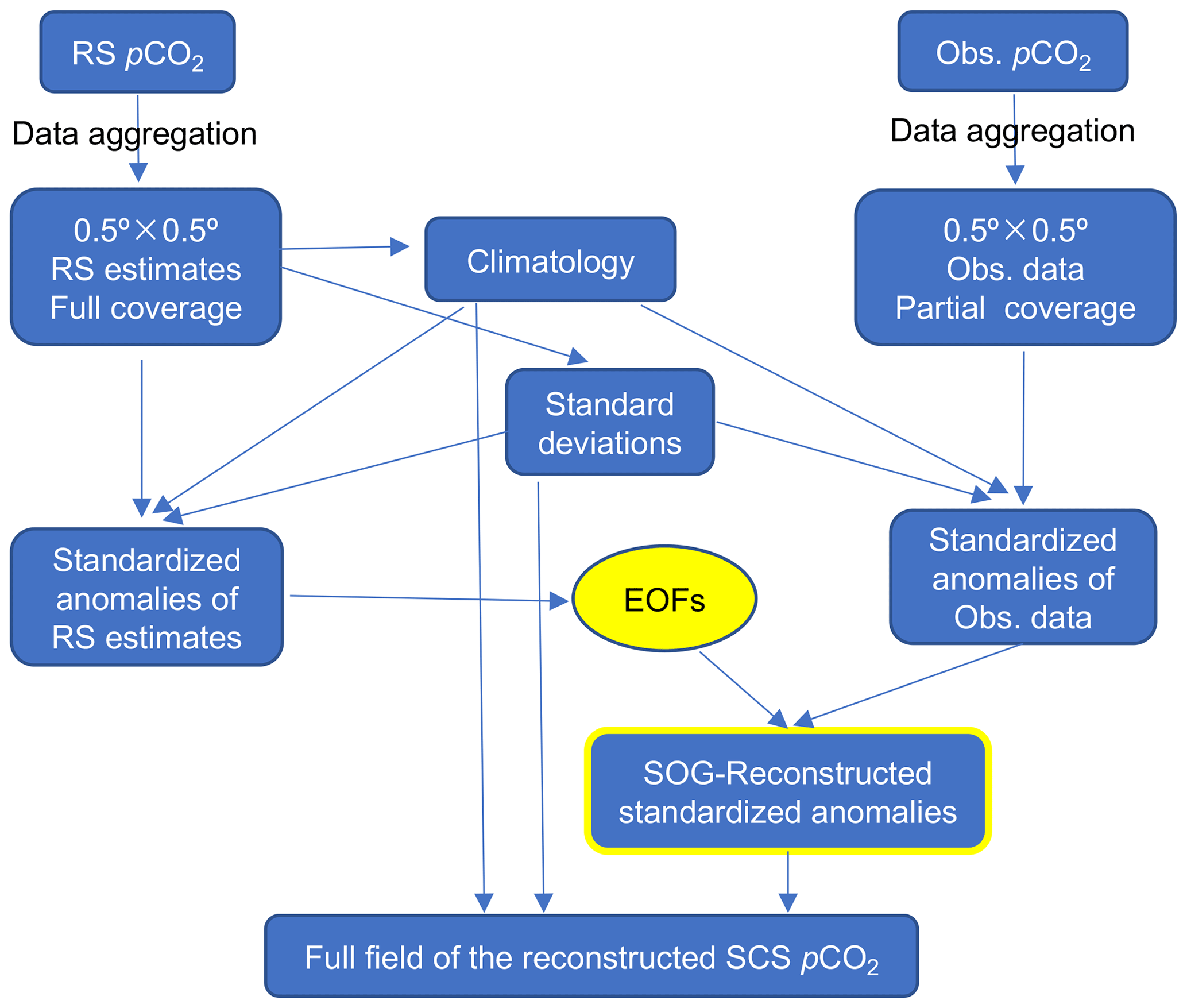
Figure 1Reconstruction procedure of the sea surface pCO2 in the SCS. Here, RS pCO2 means the original remote-sensing-derived pCO2; Obs. pCO2 represents the original observed in situ pCO2. RS estimates are the grid-aggregated remote-sensing-derived pCO2, and Obs. data are the grid-aggregated observed pCO2. The standard deviations are the temporal standard deviation of the RS pCO2 estimates on each grid box.
Section 2 will describe the datasets and methods; Sect. 3 includes results and discussion; and the conclusions are in Sect. 4.
2.1 Observed data in the SCS
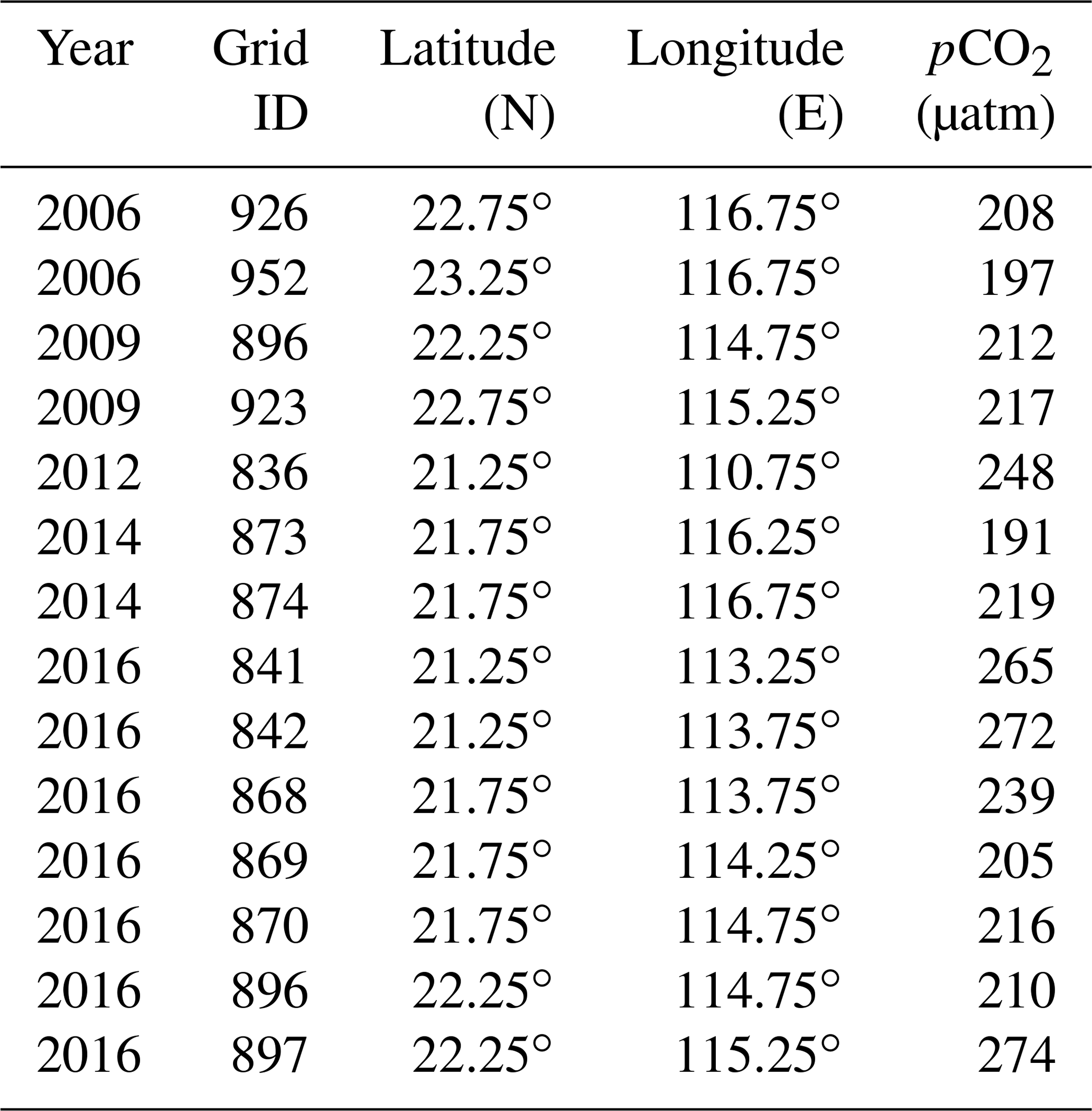
In the SCS, the underway sea surface pCO2 data are hardly available for every month of each year, so we decided to compile the data seasonally. This study focuses on the summer data, since the greatest temporal coverage of the sampling occurs in summer. The available underway summer pCO2 data from 2000 to 2017 are compiled in this study and shown in Table 1, in which the pCO2 data in August 2004, July 2005, and June 2006 are new and obtained continuously with a non-dispersive infrared gas analyzer (LI-COR 7000). The summer data are the June–August mean for each year in this period excluding 2002, 2003, 2010, 2011, and 2013 (Li et al., 2020; Zhai et al., 2005a). Thus, we have observed underway pCO2 data for 13 summers during 2000–2017. Figure 2 shows that these data are distributed mainly on the northern shelf and slope and in the northern and mid basin of the SCS with a different frequency of summer observations on different grid boxes. The observational data were aggregated onto grid boxes in the 5–25∘ N, 109–122∘ E region of the SCS. The aggregation used a simple space–time average of the data in a grid box. The aggregated data for the 13 summers are shown in Fig. 3, which shows the distribution pattern of the observed underway pCO2 data of each year. The aggregated pCO2 in general falls in the range of 160–480 µatm with relatively larger spatial variation nearshore and smaller spatial variability in the basin. In addition, the large differences are apparent in the spatial coverage from year to year. For example, in the summer of 2007 the observed underway pCO2 data cover a spatial range of 12∘ in latitude and 13∘ in longitude, with 231 grid boxes with data that cover 22 % of the SCS. The data fall in the range of 281–480 µatm. In the summer of 2017 the observed data cover a spatial range of 13∘ in latitude and 6∘ in longitude, with 77 grid boxes with data that cover 7 % of the SCS. The data are in the range of 279–440 µatm. The summer of 2000 has only five grid boxes (covering 0.5 % of the SCS) with data in the range of 400–425 µatm. The lowest observational pCO2 values appear on the northern SCS shelf due to the influence of the Pearl River plume (see Fig. 2), where nutrient-stimulated phytoplankton uptake consumes CO2. The relatively high sea surface pCO2 values occur mainly in the basin, which are often higher than the atmospheric pCO2 (Li et al., 2020; Zhai et al., 2013). The high pCO2 values off the northeastern coast of the SCS and the southern coast of Hainan Island in the summer of 2007 are consistent with local upwelling occurrences, which bring CO2-enriched water from the subsurface (Li et al., 2020). In the summer of 2012, the spatial coverage is 7∘ in latitude and 9.5∘ in longitude. The pCO2 data are in the range of 191–480 µatm with the lowest value appearing on the northwestern shelf of the SCS due to the Jianjiang River plume and the highest values occurring on the northeastern shelf and off the eastern coast of Hainan Island due to upwelling (Gan et al., 2015; Jing et al., 2015). Some other data, for example, in the summer of 2000, however, are relatively localized so that no certain spatial pattern is shown before the reconstruction. Our reconstruction results will help display the spatial patterns of the complete sea surface pCO2 field.
Table 1Underway sea surface pCO2 data in summer in the SCS compiled in this study.
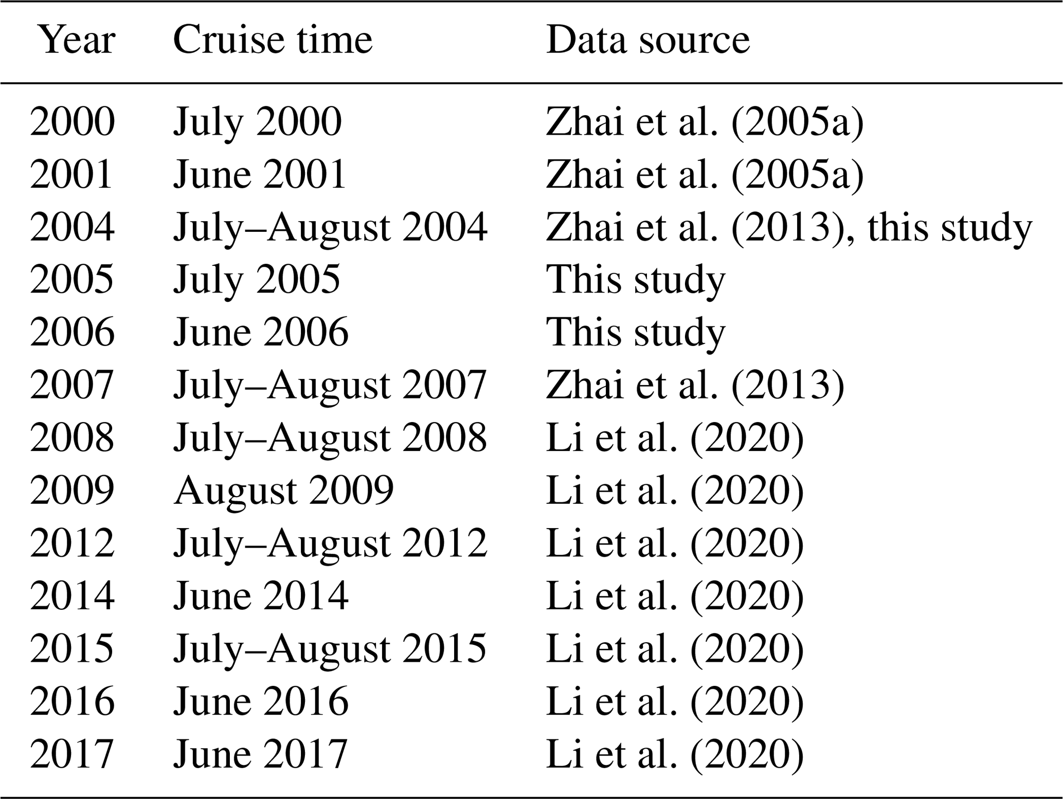

Figure 2The number of summers with underway sea surface pCO2 observations in the SCS in the years 2000–2017. HI represents Hainan Island; Jian. R. is the Jianjiang River; and Pearl R. represents the Pearl River.
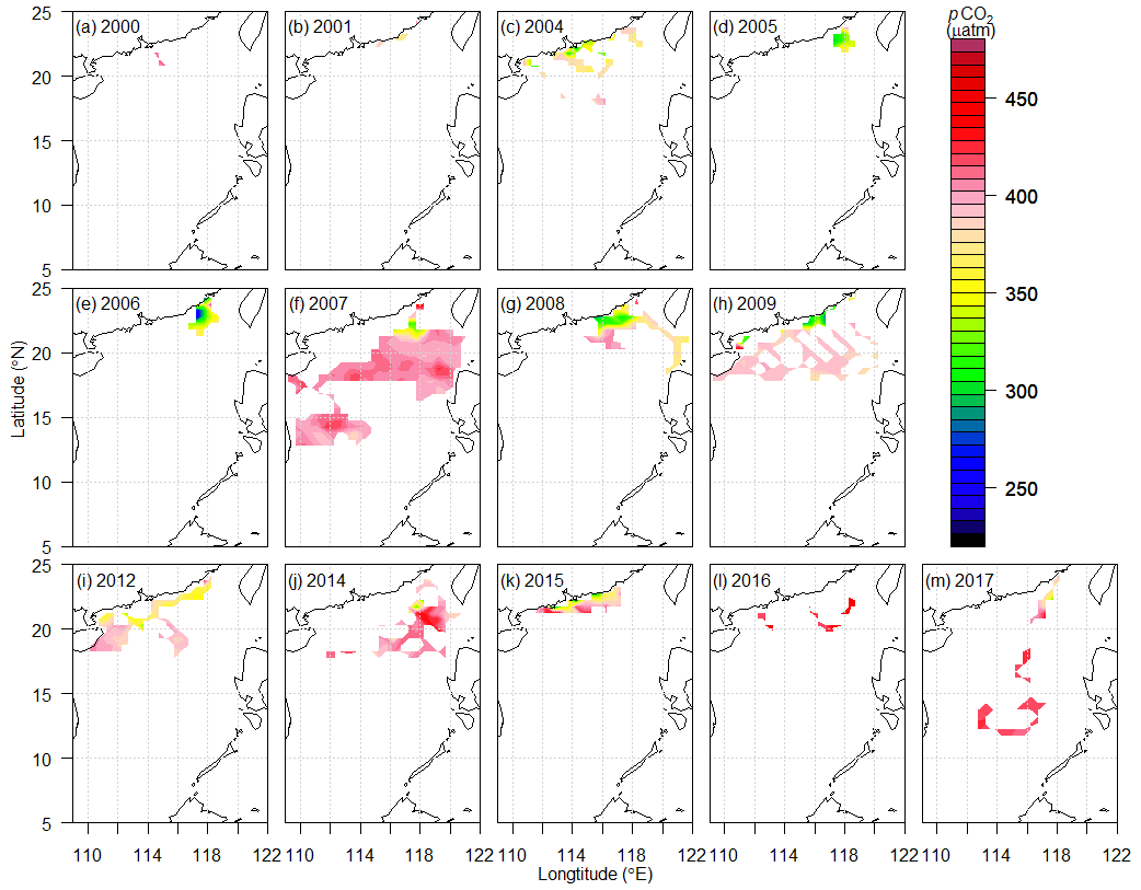
Figure 3The aggregated in situ observational pCO2 data in grid boxes in the SCS in the 13 summers during the years 2000–2017.
As a dataset for our reconstruction validation, we calculated the sea surface pCO2 from the observed temperature, salinity, total alkalinity, dissolved inorganic carbon, phosphate, and silicate at Station SEATS (SouthEast Asia Time-series Study; 18∘ N, 116∘ E) in the northern basin of the SCS in the summer of 2007, 2009, 2012, 2014, and 2017. The nutrient sample collection and measurement are described in Du et al. (2013, 2017). The samples of total alkalinity and dissolved inorganic carbon were collected and measured following the same procedure in Guo et al. (2015). The calculation of pCO2 was made using the program of Lewis and Wallace (1998), in which the apparent dissociation constants for carbonic acid of Mehrbach et al. (1973) refit by Dickson and Millero (1987) and the dissociation constant for bisulfate ion from Dickson (1990) were employed. Another sea surface pCO2 dataset calculated in the same way at Station SEATS in the summer of 2000, 2001, 2004, and 2006 was compiled from Lui et al. (2020).
2.2 Remote-sensing-derived sea surface pCO2 data
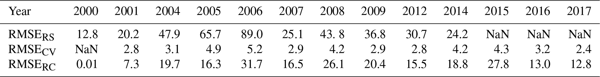
The satellite remote-sensing-derived sea surface pCO2 in the SCS was estimated for the years of 2000–2014 using a “mechanistic semi-analytical algorithm” (MeSAA) developed by Bai et al. (2015a). In the summer in the SCS, the thermodynamic, mixing, and biological effects on the sea surface pCO2 were parameterized in the MeSAA algorithm as a function of major controlling factors derived from multiple-satellite-derived sea surface temperature, colored dissolved organic matter, and chlorophyll. The spatial resolution of the remote-sensing-derived pCO2 estimates is . These estimates were aggregated into grid boxes in our study region (5–25∘ N, 109–122∘ E). As shown in Fig. 4, the gridded remote-sensing-derived pCO2 data cover almost all the areas of the SCS (see the boxes of RS pCO2 and RS estimates of full coverage in Fig. 1). We made a validation study for the remote-sensing-derived pCO2 by comparison with the observed underway pCO2 (Fig. 5). In general, most of the remote-sensing-derived pCO2 overestimate the sea surface pCO2 but not by more than 50 µatm. The root-mean-square error (RMSE) falls in the range from 12.8 to 89.0 µatm with a median of 33.8 µatm (Table 2). The RMSE values are high in the years when the underway data covered only the shelf regions. With the MeSAA algorithm, the derived pCO2 dataset represents the major CO2 variation in large scales. However, variations shown by these remote-sensing-derived pCO2 data are much less than those shown by the observed pCO2 data because the current MeSAA algorithm does not consider some local processes, such as eddies and potentially different carbonate system patterns in coastal areas. Larger spatial variations are expected especially in areas influenced by river plumes. This makes it necessary to reconstruct a pCO2 field not only from the remote-sensing-derived pCO2 but also constrained by the observed in situ pCO2 data from cruises.
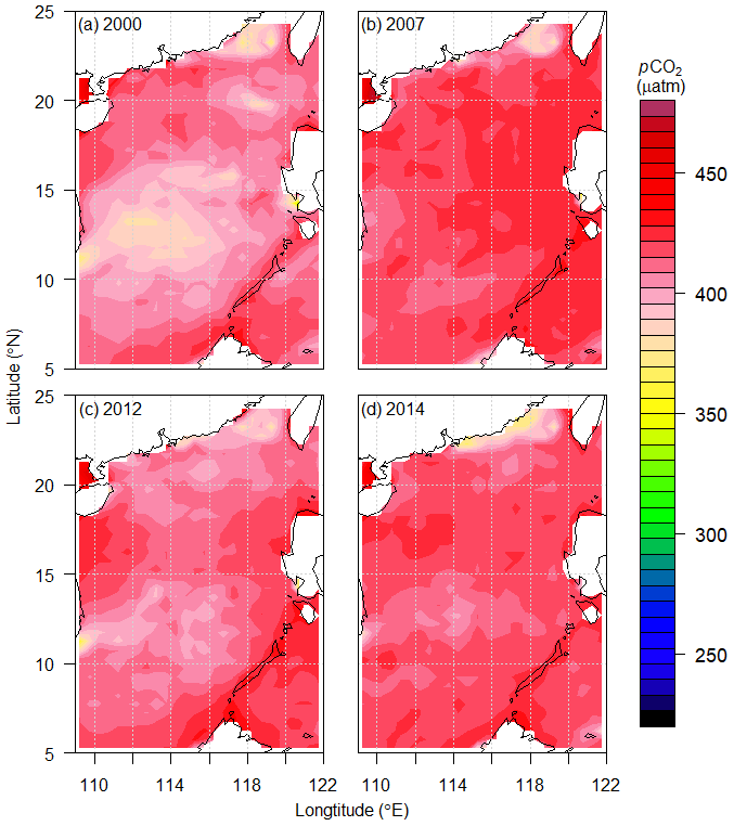
Figure 4Remote-sensing-derived sea surface pCO2 in summer in selected years from 2000 to 2014.
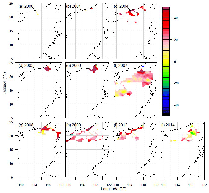
Figure 5The difference between the remote-sensing-derived summer pCO2 estimates and the observed underway pCO2 (unit: µatm) in 2000, 2001, 2004–2009, 2012, and 2014.
Table 2The RMSE between the remote-sensing-derived pCO2 estimates and the observed underway pCO2 data (RMSERS), of the cross-validation (RMSECV), and between the reconstructed pCO2 and the observed underway pCO2 data (RMSERC) (unit: µatm).
2.3 Reconstruction method
Figure 1 is a flowchart of our method. We used the remote-sensing-derived data to compute the EOFs for the SOG reconstruction. The grid with resolution covered 5–25∘ N and 109–122∘ E with 1040 grid boxes in total. The land area data were marked with NaN. The data were arranged in a 1040×15 space–time matrix with rows for grid boxes and columns for time. Then, we removed the 143 land grid boxes from the data and computed the climatology and standard deviation for the remaining 897 non-NaN grid boxes from the 15 years of remote-sensing-derived data from 2000 to 2014. The standardized anomalies were computed for each grid box using the remote-sensing-derived data minus the climatology and subsequently dividing the difference by the standard deviation. The singular-value decomposition (SVD) method was applied to the standardized anomalies in the space–time matrix to compute the EOFs. The results are shown in Sect. 3. The climatology and standard deviation calculated from the remote-sensing-derived data were also used to compute the standardized anomalies of the observed data, which were used as the response variable in the SOG regression reconstruction. Following the reconstruction of the standardized anomalies, the remote-sensing-derived climatology and standard deviation were then used to produce the full field as the final reconstruction result.
The SOG reconstruction method is basically a multilinear regression model for the space–time field at grid box x and time t, expressed as follows:
where P(x,t) is the response variable whose data are the standardized anomalies of the observed data, β0(t) is the regression intercept, βm(t) is the regression coefficient for the mth EOF Em(x), the least-square estimator of βm(t) is denoted by bm(t), a(x)=cos (ϕx) is the area factor, ϕx is the centroid's latitude (expressed in radians) of the grid box x, and e(x,t) is the regression error. The error is assumed to be normally distributed with a zero mean and has an independent error variance of
where E denotes the mathematical operation of the expected value. The explanatory variables in the above multilinear regression are Em(x), computed from the area-weighted standardized anomalies of the remote-sensing-derived data. The anomalies were written as an 897×15 space–time data matrix. The SVD method was applied to this matrix to compute the spatial patterns, which are EOFs; the temporal patterns, which are principal components (PCs); and their corresponding variances. M is the set of EOFs selected for our regression reconstruction. It contained eight EOFs for every year except 2000, which had only four EOFs because the year had only five grid boxes with observed underway data.
For a given year, the grid boxes with observed data are known. Then, the linear regression model can be computed based on the observed data P(xd,t) and the EOFs in the grid boxes xd with the observed data Em(xd). For example, the year 2002 had only 17 grid boxes with the observational data: . The data in these 17 boxes were used to estimate the intercept β0(t) and coefficients βm(t) of the regression. With the estimates b0(t) and bm(t), m∈M, the reconstructed standardized anomalies are expressed as
where x runs through the entire 893 grid boxes over our study region in the SCS. These anomalies were converted to the full field by adding the climatology and multiplying the standard deviation computed from the remote-sensing-derived data for each of the 893 grid boxes. In this way, the full reconstructed field was produced and is presented in Sect. 3.
Many computer software packages are available to compute the EOFs using SVD and to compute multilinear regressions. This paper chose to use R, a computer program language that has become a popular data science tool in the last few years, for this purpose.
SOG usually uses the first few EOFs or the first M EOFs that account for more than 80 % of the total variance or that are determined by response data via a correlation test (Smith et al., 1998). Here, M is the size of set M. The current paper used eight EOFs that explain 87 % of the total variances (Fig. 6).
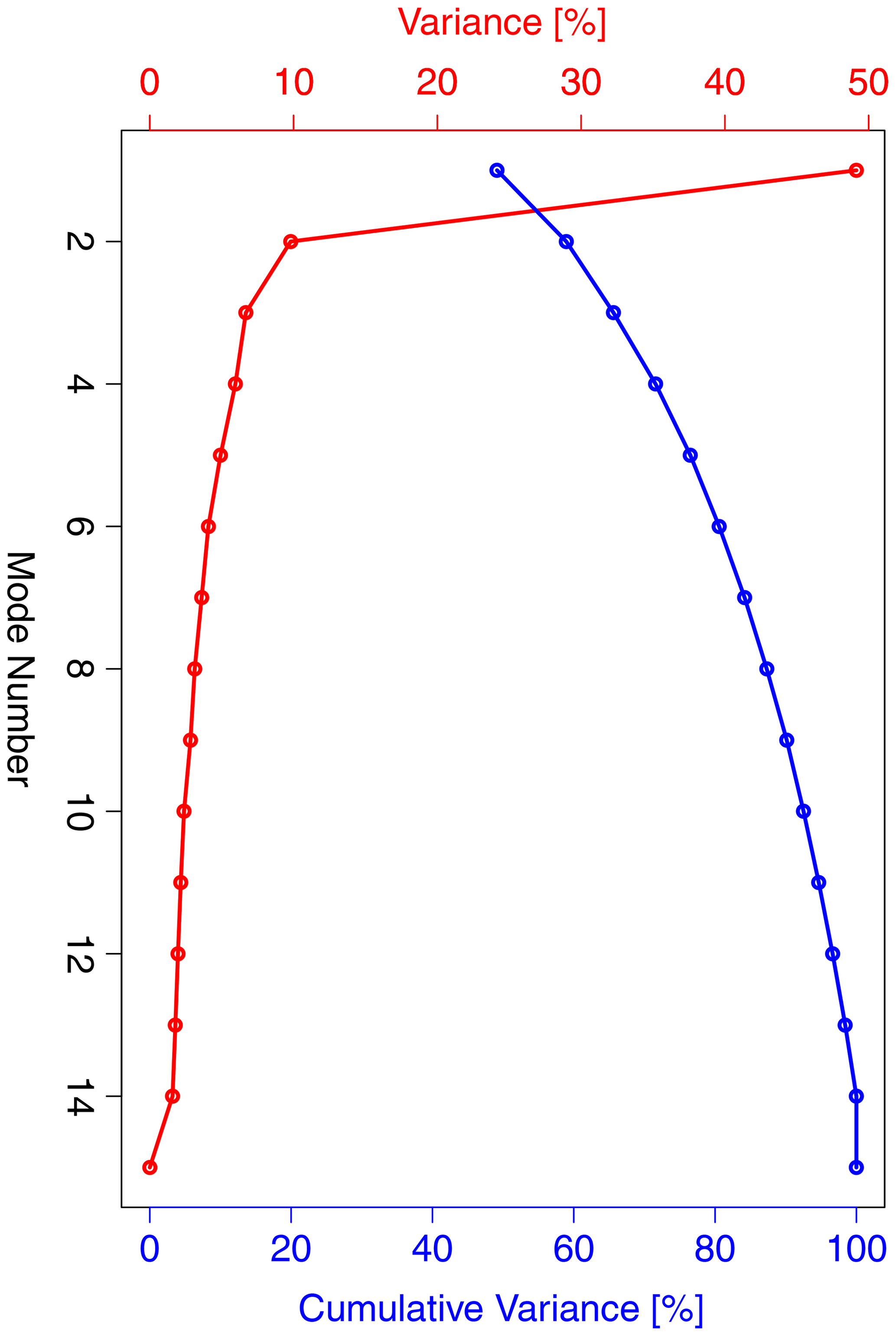
Figure 6The percentage variances and cumulative variances based on the summer remote-sensing-derived pCO2 data for the period of 2000–2014.
3.1 EOFs and PCs
EOF1 demonstrates the mode of an average level of pCO2 with lower or higher values near the coastal regions of mainland China (Fig. 7a). This mode accounts for 49 % of the variance, which indicates the dominance of the average field and hence a small overall spatial variation, except in the coastal regions. The remote-sensing-derived pCO2 data support this mode well. EOF2 shows a north–south dipole (Fig. 7b), which is supported by the observed data shown in Fig. 3, particularly in the summer of 2017, showing lower values in the north on the shelf and slope and higher values in the south in the ocean basin. The minimum values in the north occur where the Pearl River plume dominates (Li et al., 2020; Zhai et al., 2013). EOF3 shows an east–west pattern (Fig. 7c), in addition to the north–south dipole in EOF2. EOF3 thus reflects a spatial variation of a smaller scale. This pattern is consistent with that influenced by coastal upwelling along the northeastern China coast and off eastern Hainan Island (Gan et al., 2015; Jing et al., 2015).
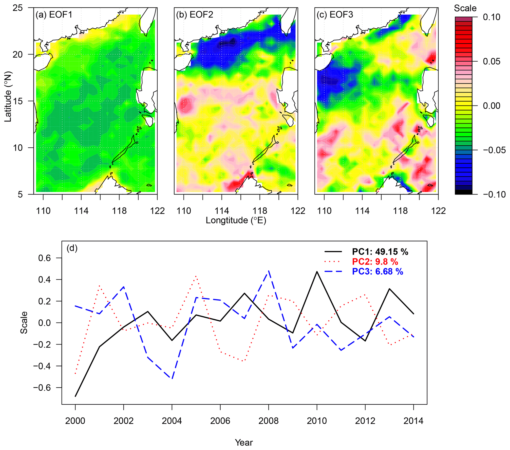
Figure 7EOFs and PCs of the remote-sensing-derived pCO2 estimates. (a–c) EOFs and (d) PCs.
The PCs are a temporal stamp of the occurrence of the spatial patterns. PC1 basically shows the temporal trend (Fig. 8d). It has been concluded that surface SCS pCO2 has an increasing trend with time (Tseng et al., 2007). PC2 indicates the strength of the north–south dipole. This strength seems to be related to the strength and extent of the Pearl River plume on the northern shelf and slope (Bai et al., 2015b; Li et al., 2020; Zhai et al., 2013). PC3 shows the temporal variation corresponding to the east–west spatial pattern of EOF3.
3.2 Reconstruction results in the SCS
Figure 8 shows that the reconstructed pCO2 fields in the SCS have successfully displayed the spatial patterns of the observed pCO2 and in general are consistent with previous studies (Li et al., 2020; Zhai et al., 2013). Relatively low values appear in the northern coastal region where the Pearl River plume is dominant in summer, and generally high values occur in the mid and southern basins.
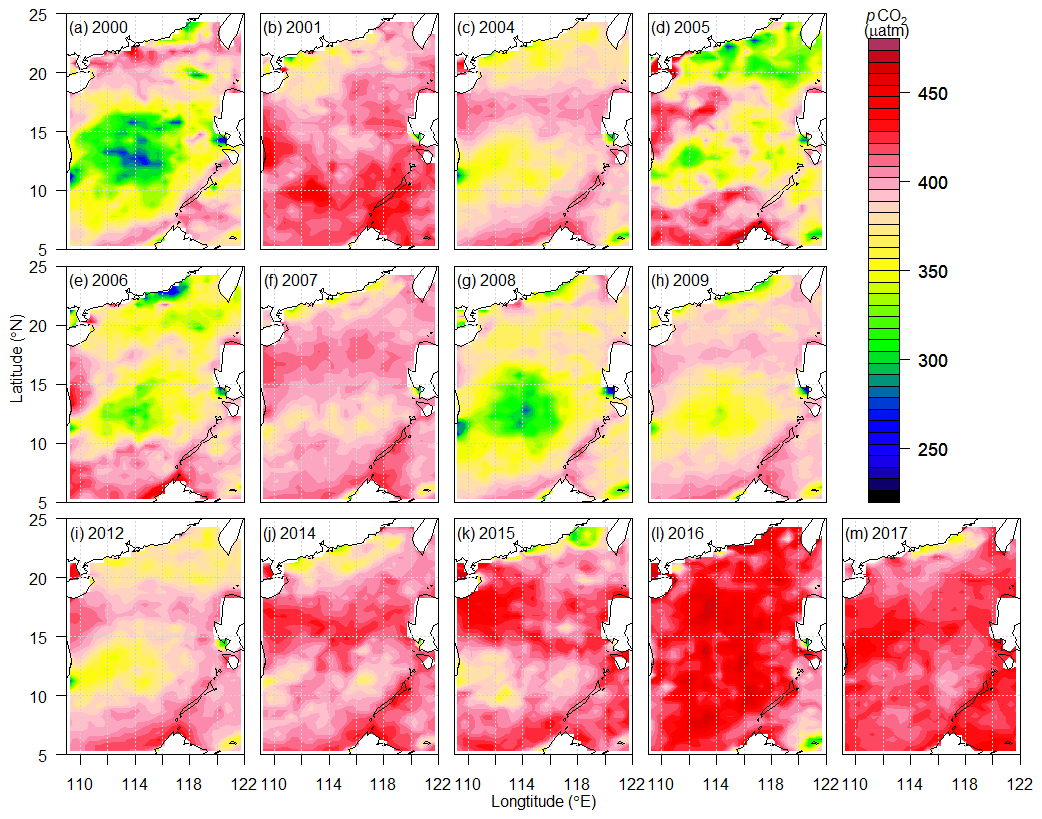
Figure 8Reconstructed summer pCO2 fields for the years 2000–2017 in the SCS.
The reconstructions have taken the advantages of both the observed underway data for retaining spatial and temporal variations and the remote-sensing-derived data for EOF patterns. By default, the reconstructed field has fidelity to the in situ data because the SOG reconstruction method is a fit of EOFs to the in situ data. The reconstruction is, thus, consistent with the in situ observations. When the in situ data cover a sufficiently large area and hence provide a proper constraint to the EOF fitting through the SOG procedure, the reconstruction result is more faithful to the reality. For example, the reconstructions of the summers of 2004, 2007, 2009, 2012, and 2014–2017 nicely demonstrate the spatial pCO2 patterns (Fig. 8c, f, h, and i–m) that are consistent with observations (Li et al., 2020; Zhai et al., 2013) and ocean dynamics (Gan et al., 2015; Jing et al., 2015).
When the observational data are scarce, as long as the in situ data provide a proper constraint to the EOFs, the reconstruction can still yield reasonable results. For example, the summer of 2001 has few in situ data, but its reconstruction, with an RMSE of 7.3 µatm between the reconstructed data and the observed data, appears reasonable (Fig. 8b).
In cases of extreme data scarcity, the reconstruction may not be reliable. For example, the reconstructed data in the summer of 2000 appear to be of poor quality (Fig. 8a), since the relatively low values in the mid-SCS basin may not be realistic. These poorly reconstructed data may be due to the poor spatial coverage of the in situ pCO2 data in the summer of 2000, which had only five grid boxes with data (Fig. 3a). These five boxes are all located together and cover only 0.5 % of the SCS. Similarly, the reconstructed pCO2 data for the summers of 2005, 2006, and 2008 are not well constrained by the in situ pCO2 data that cover only the northern shelf and slope of the SCS so that the reconstructed pCO2 in the mid basin are less than 350 µatm (Figs. 8d, e, and g). These small values are unlikely, since the sea surface pCO2 in the basin is generally higher than the atmospheric pCO2 (380–420 µatm) (Li et al., 2020; Zhai et al., 2013). Another cause of the less ideal reconstruction results for the summers of 2005, 2006, and 2008 may be the large spatial variations in the in situ data. These variations, such as those for the summer of 2008 (Fig. 3g), in the in situ data can cause a large deviation of the regression coefficients because the linear regression is not robust.
The reconstruction results have demonstrated the feasibility of the SOG reconstruction of the sea surface pCO2 over the SCS, as long as the in situ data provide a proper constraint to the EOFs. The percentage of the in situ data coverage needs not necessarily be large. However, large spatial variations in the in situ data can distort the reconstruction and lower the quality of reconstruction because the linear regression method is not robust.
3.3 Reconstruction validation and uncertainty quantification
To quantitatively validate our reconstruction, we conducted a leave-one-out cross-validation study: withholding a grid box datum, making the reconstruction using the remaining in situ data, and computing the difference between the withheld datum and the reconstructed datum at the same grid box. This was repeated for every grid box with in situ data for each year. The final cross-validation result is output as RMSE (Table 2). The maximum RMSE is 5.2 µatm, which occurred in 2006 when there were only 25 grid boxes with in situ pCO2 data, and the in situ data had the largest spatial standard deviation, 49.4 µatm, among the 13 years under consideration. The minimum RMSE is 2.4 µatm, which occurred in 2017 with 77 in situ data grid boxes and a spatial standard deviation of 17.6 µatm for the in situ data. This accuracy is very good compared to the spatial standard deviation of the in situ data in the same year. Compared to the 2006 data, a more accurate reconstruction for 2017 is expected because of more grid boxes with in situ data and smaller spatial variability. This is supported by the cross-validation result. The spatial standard deviation of the reconstructed data is in the range of 2.1–6.6 µatm. The cross-validation RMSEs are in the range of 2.4–5.2 µatm. We thus conclude that the reliability of our reconstruction is well supported by the leave-one-out cross-validation result.
We have also considered other types of cross-validations, such as leaving out data in half of the study region. A numerical test was made for the following situation: leaving out the western or eastern half of the data in a year, making the reconstruction using the remaining half of data, and computing the RMSE between the removed data and the reconstructed data. The analysis was done for the years with better spatial coverage: 2007, 2009, and 2012. When the western halves (longitude<115.5∘ E) of data in these years were removed, the resulted RMSEs were 2.77, 4.46, and 3.82 µatm for 2007, 2009, and 2012, respectively. When the eastern halves (longitude>115.5∘ E) of data were removed, the RMSEs were 4.32, 3.66, and 3.55 µatm in 2007, 2009, and 2012, respectively. These RMSEs fall within the range of the RMSEs of the leave-one-out cross-validation. These numerical results are another confirmation of the reliability of our reconstruction.
The uncertainty in our reconstruction was quantified by grid-by-grid comparisons of the reconstructed pCO2 with the observed pCO2 in two ways. One is the comparison with the observed underway data (Fig. 9). The difference between the reconstructed data and the observed underway data mostly falls within the range from −30 to 30 µatm (Fig. 9). The greatest deviation from the underway data appears near the coast, likely due to the lack of some typical patterns in coastal areas transferred via EOFs from the remote sensing estimates. The RMSE between the reconstructed data and the observed underway data is no larger than 31.7 µatm with a median of 16.5 µatm, which is smaller than the RMSE between the remote-sensing-derived pCO2 and the underway data with the relative difference between the two RMSEs (rows 1 and 3 in Table 2) by at least 29 %. When comparing the pCO2 data produced by Jo et al. (2012) in the northern SCS by a neural network approach in the summer of the years 2004–2007 with the underway pCO2, the resultant RMSE falls in the range from 32.6 to 44.5 µatm and is twice as much as the median RMSE between our reconstructed pCO2 and the underway pCO2 (Table 2). Another uncertainty quantification for our reconstruction is to compare it with the pCO2 calculated from long-term observations at Station SEATS (Fig. 10). The difference between the reconstructed pCO2 and the observed data at Station SEATS ranges from −7 to 10 µatm with the relative difference from −1.5 % to 2.1 %. Both comparisons confirm that our reconstruction results are reliable.
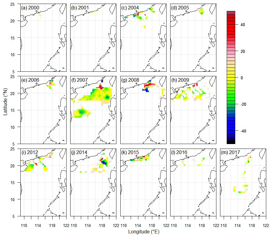
Figure 9The difference between the reconstructed summer pCO2 and the observed underway pCO2 (unit: µatm) in 2000, 2001, 2004–2009, 2012, and 2014–2017.
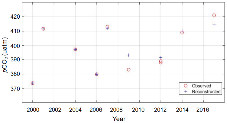
Figure 10The comparison between the summer sea surface pCO2 calculated from the observations and those from our reconstruction at Station SEATS (18∘ N, 116∘ E). The pCO2 data calculated from the observations in the years of 2000, 2001, 2004, and 2006 are from Lui et al. (2020).
As an application of our reconstruction and a validation, we examine the temporal trend of sea surface pCO2 over the SCS. The rate based on the linear temporal trend of the spatial average of the reconstructed sea surface pCO2 over the SCS from 2000 to 2017 is 2.4±0.8 µatm yr−1 (see Fig. 11a). It is lower than the rate of fCO2 increase (4 µatm yr−1) for the period of 1999–2003 (Tseng et al., 2007), while it is higher than the rate of pCO2 increase for the period of 1998–2006 (0.8 µatm yr−1) at Station SEATS (Lui et al., 2020). The differences between their rates and ours exist because (a) our rate is a spatial average in summer and their rates are based on data collected in spring, summer, fall, and winter at a basin station and (b) the period to derive our rate is much longer than theirs. Using the summer data in Lui et al. (2020), the rate we estimated from the year 2000, which is the beginning year of our data, to the year 2006 at Station SEATS is 2.5±1.0 µatm yr−1. Although the period of 2000–2006 is much shorter than our period of 2000–2017, the summer rate at Station SEATS is almost the same as our rate based on the reconstructed data over the SCS. When compared with the summer rate of observed pCO2 at Station ALOHA (A Long-Term Oligotrophic Habitat Assessment station) ( N, 158∘ W) in the North Pacific, which is 2.0±0.2 µatm yr−1 over 2000–2017 (Dore et al., 2009) (see Fig. 11b), our rate is consistent with the rate in the North Pacific. The consistency of the trend in our reconstructed sea surface pCO2 over the SCS with the local trend at Station SEATS and the North Pacific trend at Station ALOHA confirms that our reconstruction is reasonable.

Figure 11(a) Time series and linear trend of the spatial averages of the reconstructed summer pCO2 data in the SCS in the period of 2000–2017; (b) summer sea surface pCO2 at Station ALOHA in the years 2000–2017 adapted from Dore et al. (2009).
3.4 Outliers of the observed data in the reconstruction
The SOG method is basically a linear regression method, which is known to be sensitive to the outliers of the response data. Some outliers, whether due to observational biases or extreme events, can cause a large change in the regression coefficients and hence the regression results and can even make the regression results outside the physically valid domain, such as negative pCO2 values in the reconstructed data. Although we cannot conclude that the outliers of 3σ away from the mean in the observed data are due to data biases, we have decided not to use them in our reconstruction to avoid the unphysical reconstruction results. Table 3 shows the 14 outlier entries excluded from our response data for regression. These outliers are located in the region of 21.25–23.25∘ N, 113.25–116.75∘ E. This region is near the Pearl River estuary. Thus, these extremely low pCO2 values may result from the Pearl River plume where the observed pCO2 can be very low. These very low values, such as those at least 3σ away from the mean, may cause a very large gradient in the observed pCO2. Our reconstruction has excluded these extremely low values influenced by the river plumes. Our reconstructed data may therefore overestimate the pCO2 values in the Pearl River estuary and its nearby region.
The R computer codes and their required files for this paper are freely available at the following link: https://doi.org/10.5281/zenodo.4567859 (Wang et al., 2021).
The gridded underway sea surface pCO2 data, the remote-sensing-derived sea surface pCO2 estimates, and the reconstruction result data are openly and freely available at PANGAEA at the following link: https://doi.org/10.1594/PANGAEA.921210 (Wang et al., 2020).
This study has demonstrated the feasibility of using the SOG method to reconstruct the sea surface pCO2 data into regular grid boxes. We compiled the observed underway and remote-sensing-derived sea surface pCO2 data in the SCS in summer over the period of 2000–2017 and aggregated these data with a grid resolution of for reconstruction. The SOG method based on the multilinear regression was applied to reconstruct the space–time complete pCO2 field in the SCS. The method took the EOFs calculated from the remote-sensing-derived pCO2 as the explanatory variables and treated the observed pCO2 as the response variable. The EOFs reflect reasonably well the general spatial pattern of the sea surface pCO2 in the SCS and reveal features affected by regional physical forcing such as the river plume and coastal upwelling in the northern SCS. As long as the in situ data provide a proper constraint to the EOFs, the reconstructed pCO2 fields are, in general, consistent with the patterns of the observed pCO2 and demonstrate relatively low values along the northern coast affected by the Pearl River plume and consistently high values in the ocean basin of the SCS. The leave-one-out cross-validation result validates our reconstruction with an RMSE smaller than the spatial standard deviation of the observed underway data in the same year. The grid-by-grid comparison of the reconstructed summer pCO2 with the observed underway pCO2 has an RMSE smaller than that of the remote-sensing-derived pCO2, as well as that of the neural-network-produced pCO2 in the same year. Moreover, our reconstructed pCO2 compares well with the pCO2 calculated from observations around Station SEATS in the northern basin of the SCS. These comparisons confirm that our reconstruction is reliable. The temporal rate of our reconstructed sea surface pCO2 over the SCS is consistent with the local rate at Station SEATS and the North Pacific rate at Station ALOHA, which further validates our reconstruction. These reconstructed pCO2 fields provide full spatial coverage of the sea surface pCO2 of the SCS in summer over a temporal scale of almost 2 decades and therefore help fill the long-lasting blanks on the global sea surface pCO2 map. Thus, the reconstruction products will help improve the accuracy of the estimate of the oceanic CO2 flux of the largest marginal sea of the western Pacific so as to better constrain the global oceanic carbon uptake capacity.
Although the SOG method can optimize the information from both the in situ data and the remote-sensing-derived data, the reliability of the reconstructed results is still limited by the observed data. When the observed data are limited to only a few grid boxes in a small region, the reconstruction results may not be realistic. Additional constraints have to be considered.
MD conceptualized and directed the field program of the in situ observations. BC and XG participated in the in situ data collection. YB provided the remote-sensing-derived data. GW, YC, and SSPS developed the reconstruction method, wrote the MATLAB and R codes, analyzed the data, and plotted the figures. ZW participated in the uncertainty analysis of the reconstruction and plotted some of the figures. HQ developed the data repository and revised and tested the R codes. GW and SSPS wrote the paper. All the authors contributed to the original writing, editing, and revisions of the paper.
The authors declare that they have no conflict of interest.
We thank Hon-Kit Lui for the communication about the data at Station SEATS. We are thankful to Weidong Zhai for providing the underway pCO2 data in his publications and to Young-Heon Jo for providing the neural-network-produced pCO2 estimates in his published paper. We appreciate the constructive comments from the two anonymous reviewers that have helped improve this paper. Aiqin Han, Tao Huang, and Lifang Wang helped in nutrient sample collection and measurements, and Liguo Guo, Wenping Jing, Yi Xu, Wei Yang, and Nan Zheng helped in the sample collection and measurements of total alkalinity and dissolved inorganic carbon at Station SEATS. The work by Guizhi Wang, Yan Bai, Xianghui Guo, and Minhan Dai was supported by grants from the Ministry of Science and Technology of China (nos. 2015CB954001 and 2009CB421200). The observed underway pCO2 data in 2004, 2005, and 2006 were collected under the support of the National Natural Science Foundation of China (grant no. 40521003).
This research has been supported by the Ministry of Science and Technology of China (grant nos. 2015CB954001 and 2009CB421200) and the National Natural Science Foundation of China (grant no. 40521003).
This paper was edited by David Carlson and reviewed by two anonymous referees.
Bai, Y., Cai, W.-J., He, X., Zhai, W. D., Pan, D., Dai, M., and Yu, P.: A mechanistic semi-analytical method for remotely sensing sea surface pCO2 in river-dominated coastal oceans: a case study from the East China Sea, J. Geophys. Res., 120, 2331–2349, https://doi.org/10.1002/2014JC010632, 2015a.
Bai, Y., Huang, T. H., He, X. Q., Wang, S. L., Hsin, Y. C., Wu, C. R., Zhai, W. D., Lui, H. K., and Chen, C. T. A.: Intrusion of the Pearl River plume into the main channel of the Taiwan Strait in summer, J. Sea Res., 95, 1–15, https://doi.org/10.1016/j.seares.2014.10.003, 2015b.
Bakker, D. C. E., Pfeil, B., Landa, C. S., Metzl, N., O'Brien, K. M., Olsen, A., Smith, K., Cosca, C., Harasawa, S., Jones, S. D., Nakaoka, S., Nojiri, Y., Schuster, U., Steinhoff, T., Sweeney, C., Takahashi, T., Tilbrook, B., Wada, C., Wanninkhof, R., Alin, S. R., Balestrini, C. F., Barbero, L., Bates, N. R., Bianchi, A. A., Bonou, F., Boutin, J., Bozec, Y., Burger, E. F., Cai, W.-J., Castle, R. D., Chen, L., Chierici, M., Currie, K., Evans, W., Featherstone, C., Feely, R. A., Fransson, A., Goyet, C., Greenwood, N., Gregor, L., Hankin, S., Hardman-Mountford, N. J., Harlay, J., Hauck, J., Hoppema, M., Humphreys, M. P., Hunt, C. W., Huss, B., Ibánhez, J. S. P., Johannessen, T., Keeling, R., Kitidis, V., Körtzinger, A., Kozyr, A., Krasakopoulou, E., Kuwata, A., Landschützer, P., Lauvset, S. K., Lefèvre, N., Lo Monaco, C., Manke, A., Mathis, J. T., Merlivat, L., Millero, F. J., Monteiro, P. M. S., Munro, D. R., Murata, A., Newberger, T., Omar, A. M., Ono, T., Paterson, K., Pearce, D., Pierrot, D., Robbins, L. L., Saito, S., Salisbury, J., Schlitzer, R., Schneider, B., Schweitzer, R., Sieger, R., Skjelvan, I., Sullivan, K. F., Sutherland, S. C., Sutton, A. J., Tadokoro, K., Telszewski, M., Tuma, M., van Heuven, S. M. A. C., Vandemark, D., Ward, B., Watson, A. J., and Xu, S.: A multi-decade record of high-quality fCO2 data in version 3 of the Surface Ocean CO2 Atlas (SOCAT), Earth Syst. Sci. Data, 8, 383–413, https://doi.org/10.5194/essd-8-383-2016, 2016.
Bakker, D. C. E., Alin, S. R., Bates, N., Becker, M., Castaño-Primo, R., Cosca, C. E., Cronin, M., Kadono, K., Kozyr, A., Lauvset, S. K., Metzl, N., Munro, D. R., Nakaoka, S., O'Brien, K. M., Ólafsson, J., Olsen, A., Pfeil, B., Pierrot, D., Smith, K., Sutton, A. J., Takahashi, T., Tilbrook, B., Wanninkhof, R., Andersson, A., Atamanchuk, D., Benoit-Cattin, A., Bott, R., Burger, E. F., Cai, W.-J., Cantoni, C., Collins, A., Corredor, J. E., Cronin, M. F., Cross, J. N, Currie, K. I., De Carlo, E. H., DeGrandpre, M. D., Dietrich, C., Emerson, S., Enright, M. P., Evans, W., Feely, R. A., García-Ibáñez, M. I., Gkritzalis, T., Glockzin, M., Hales, B., Hartman, S. E., Hashida, G., Herndon, J., Howden, S. D., Humphreys, M. P., Hunt, C. W., Jones, S. D., Kim, S., Kitidis, V., Landa, C. S, Landschützer, P., Lebon, G. T., Lefèvre, N., Lo Monaco, C., Luchetta, A., Maenner Jones, S., Manke, A. B., Manzello, D., Mears, P., Mickett, J., Monacci, N. M., Morell, J. M., Musielewicz, S., Newberger, T., Newton, J., Noakes, S., Noh, J.-H., Nojiri, Y., Ohman, M., Ólafsdóttir, S., Omar, A. M., Ono, T., Osborne, J., Plueddemann, A. J., Rehder, G., Sabine, C. L, Salisbury, J. E., Schlitzer, R., Send, U., Skjelvan, I., Sparnocchia, S., Steinhoff, T., Sullivan, K. F., Sutherland, S. C., Sweeney, C., Tadokoro, K., Tanhua, T., Telszewski, M., Tomlinson, M., Tribollet, A., Trull, T., Vandemark, D., Wada, C., Wallace, D. W. R., Weller, R. A., and Woosley, R. J.: Surface Ocean CO2 Atlas Database Version 2020 (SOCATv2020) (NCEI Accession 0210711), NOAA National Centers for Environmental Information, https://doi.org/10.25921/4xkx-ss49, 2020.
Boutin, J., Etcheto, J., Dandonneau, Y., Bakker, D. C. E., Feely, R. A., Inoue, H. Y., Ishii, M., Ling, R. D., Nightingale, P. D., Metzl, N., and Wanninkhof, R.: Satellite sea surface temperature: a powerful tool for interpreting in situ pCO2 measurements in the equatorial Pacific Ocean, Tellus B, 51, 490–508, https://doi.org/10.1034/j.1600-0889.1999.00025.x, 1999.
Chou, W. C., Sheu, D. D. D., Chen, C. T. A., Wang, S. L., and Tseng, C. M.: Seasonal variability of carbon chemistry at the SEATS time-series site, northern South China Sea between 2002 and 2003, Terr. Atmos. Ocean. Sci., 16, 445–465, https://doi.org/10.3319/TAO.2005.16.2.445(O), 2005.
Denvil-Sommer, A., Gehlen, M., Vrac, M., and Mejia, C.: LSCE-FFNN-v1: a two-step neural network model for the reconstruction of surface ocean pCO2 over the global ocean, Geosci. Model Dev., 12, 2091–2105, https://doi.org/10.5194/gmd-12-2091-2019, 2019.
DeVries, T., Le Quere, C., Andrews, O., Berthet, S., Hauck, J., Ilyina, T., Landschutzer, P., Lenton, A., Lima, I. D., Nowicki, M., Schwinger, J., and Seferian, R.: Decadal trends in the ocean carbon sink, P. Natl. Acad. Sci. USA, 116, 11646–11651, https://doi.org/10.1073/pnas.1900371116, 2019.
Dickson, A. G.: Standard potential of the reaction: , and the standard acidity constant of the ion in synthetic sea water from 273.15 to 318.15 K, J. Chem. Thermodyn., 22, 113–127, https://doi.org/10.1016/0021-9614(90)90074-Z, 1990.
Dickson, A. G. and Millero, F. J.: A comparison of the equilibrium constants for the dissociation of carbonic acid in seawater media, Deep-Sea Res. Pt. I, 34, 1733–1743, https://doi.org/10.1016/0198-0149(87)90021-5, 1987.
Doney, S. C., Tilbrook, B., Roy, S., Metzl, N., Le Quere, C., Hood, M., Feely, R. A., and Bakker, D.: Surface-ocean CO2 variability and vulnerability, Deep-Sea Res. Pt. II, 56, 504–511, https://doi.org/10.1016/j.dsr2.2008.12.016, 2009.
Dore, J. E., Lukas, R., Sadler, D. W., Church, M. J., and Karl, D. M.: Physical and biogeochemical modulation of ocean acidification in the central North Pacific, P. Natl. Acad. Sci. USA, 106, 12235–12240, https://doi.org/10.1073/pnas.0906044106, 2009.
Du, C., Liu, Z., Dai, M., Kao, S.-J., Cao, Z., Zhang, Y., Huang, T., Wang, L., and Li, Y.: Impact of the Kuroshio intrusion on the nutrient inventory in the upper northern South China Sea: insights from an isopycnal mixing model, Biogeosciences, 10, 6419–6432, https://doi.org/10.5194/bg-10-6419-2013, 2013.
Du, C. J., Liu, Z. Y., Kao, S. J., and Dai, M. H.: Diapycnal Fluxes of Nutrients in an Oligotrophic Oceanic Regime: The South China Sea, Geophys. Res. Lett., 44, 11510–11518, https://doi.org/10.1002/2017gl074921, 2017.
Fay, A. R. and McKinley, G. A.: Global trends in surface ocean pCO2 from in situ data, Global Biogeochem. Cy., 27, 541–557, https://doi.org/10.1002/gbc.20051, 2013.
Friedlingstein, P., O'Sullivan, M., Jones, M. W., Andrew, R. M., Hauck, J., Olsen, A., Peters, G. P., Peters, W., Pongratz, J., Sitch, S., Le Quéré, C., Canadell, J. G., Ciais, P., Jackson, R. B., Alin, S., Aragão, L. E. O. C., Arneth, A., Arora, V., Bates, N. R., Becker, M., Benoit-Cattin, A., Bittig, H. C., Bopp, L., Bultan, S., Chandra, N., Chevallier, F., Chini, L. P., Evans, W., Florentie, L., Forster, P. M., Gasser, T., Gehlen, M., Gilfillan, D., Gkritzalis, T., Gregor, L., Gruber, N., Harris, I., Hartung, K., Haverd, V., Houghton, R. A., Ilyina, T., Jain, A. K., Joetzjer, E., Kadono, K., Kato, E., Kitidis, V., Korsbakken, J. I., Landschützer, P., Lefèvre, N., Lenton, A., Lienert, S., Liu, Z., Lombardozzi, D., Marland, G., Metzl, N., Munro, D. R., Nabel, J. E. M. S., Nakaoka, S.-I., Niwa, Y., O'Brien, K., Ono, T., Palmer, P. I., Pierrot, D., Poulter, B., Resplandy, L., Robertson, E., Rödenbeck, C., Schwinger, J., Séférian, R., Skjelvan, I., Smith, A. J. P., Sutton, A. J., Tanhua, T., Tans, P. P., Tian, H., Tilbrook, B., van der Werf, G., Vuichard, N., Walker, A. P., Wanninkhof, R., Watson, A. J., Willis, D., Wiltshire, A. J., Yuan, W., Yue, X., and Zaehle, S.: Global Carbon Budget 2020, Earth Syst. Sci. Data, 12, 3269–3340, https://doi.org/10.5194/essd-12-3269-2020, 2020.
Gan, J., Wang, J., Liang, L., Li, L., and Guo, X.: A modeling study of the formation, maintenance, and relaxation of upwelling circulation on the Northeastern South China Sea shelf, Deep-Sea Res. Pt. II, 117, 41–52, https://doi.org/10.1016/j.dsr2.2013.12.009, 2015.
Gao, J., Shen, S. S. P., Yao, T., Tafolla, N., Risi, C., and He, Y.: Reconstruction of precipitation δ18O over the Tibetan Plateau since 1910, J. Geophys. Res.-Atmos., 120, 4878–4888, https://doi.org/10.1002/2015JD023233, 2015.
Guo, X. H. and Wong, G. T. F.: Carbonate chemistry in the Northern South China Sea Shelf-sea in June 2010, Deep-Sea Res. II, 117, 119–130, https://doi.org/10.1016/j.dsr2.2015.02.024, 2015.
Jing, Z., Qi, Y., Du, Y., Zhang, S. W., and Xie, L. L.: Summer upwelling and thermal fronts in the northwestern South China Sea: observational analysis of two mesoscale mapping surveys, J. Geophys. Res., 120, 1993–2006, https://doi.org/10.1002/2014jc010601, 2015.
Jo, Y.-H., Dai, M., Zhai, W., Yan, X.-H., and Shang, S.: On the variations of sea surface pCO2 in the northern South China Sea: A remote sensing based neural network approach, J. Geophys. Res., 117, C08022, https://doi.org/10.1029/2011JC007745, 2012.
Lammlein, L. J. and Shen, S. S. P.: A multivariate regression reconstruction of the quasi-global annual precipitation on 1-degree grid from 1900 to 2015, Advances in Data Science and Adaptive Analysis, 10, 185008, https://doi.org/10.1142/S2424922X18500080, 2018.
Landschutzer, P., Gruber, N., Bakker, D. C. E., and Schuster, U.: Recent variability of the global ocean carbon sink, Global Biogeochem. Cy., 28, 927–949, https://doi.org/10.1002/2014gb004853, 2014.
Laruelle, G. G., Landschützer, P., Gruber, N., Tison, J.-L., Delille, B., and Regnier, P.: Global high-resolution monthly pCO2 climatology for the coastal ocean derived from neural network interpolation, Biogeosciences, 14, 4545–4561, https://doi.org/10.5194/bg-14-4545-2017, 2017.
Lefevre, N. and Taylor, A.: Estimating pCO2 from sea surface temperatures in the Atlantic gyres, Deep-Sea Res. Pt. I, 49, 539–554, https://doi.org/10.1016/s0967-0637(01)00064-4, 2002.
Le Quéré, C., Takahashi, T., Buitenhuis, E. T., Rodenbeck, C., and Sutherland, S. C.: Impact of climate change and variability on the global oceanic sink of CO2, Global Biogeochem. Cy., 24, GB4007, https://doi.org/10.1029/2009GB003599, 2010.
Le Quéré, C., Andrew, R. M., Friedlingstein, P., Sitch, S., Hauck, J., Pongratz, J., Pickers, P. A., Korsbakken, J. I., Peters, G. P., Canadell, J. G., Arneth, A., Arora, V. K., Barbero, L., Bastos, A., Bopp, L., Chevallier, F., Chini, L. P., Ciais, P., Doney, S. C., Gkritzalis, T., Goll, D. S., Harris, I., Haverd, V., Hoffman, F. M., Hoppema, M., Houghton, R. A., Hurtt, G., Ilyina, T., Jain, A. K., Johannessen, T., Jones, C. D., Kato, E., Keeling, R. F., Goldewijk, K. K., Landschützer, P., Lefèvre, N., Lienert, S., Liu, Z., Lombardozzi, D., Metzl, N., Munro, D. R., Nabel, J. E. M. S., Nakaoka, S., Neill, C., Olsen, A., Ono, T., Patra, P., Peregon, A., Peters, W., Peylin, P., Pfeil, B., Pierrot, D., Poulter, B., Rehder, G., Resplandy, L., Robertson, E., Rocher, M., Rödenbeck, C., Schuster, U., Schwinger, J., Séférian, R., Skjelvan, I., Steinhoff, T., Sutton, A., Tans, P. P., Tian, H., Tilbrook, B., Tubiello, F. N., van der Laan-Luijkx, I. T., van der Werf, G. R., Viovy, N., Walker, A. P., Wiltshire, A. J., Wright, R., Zaehle, S., and Zheng, B.: Global Carbon Budget 2018, Earth Syst. Sci. Data, 10, 2141–2194, https://doi.org/10.5194/essd-10-2141-2018, 2018a.
Le Quéré, C., Andrew, R. M., Friedlingstein, P., Sitch, S., Pongratz, J., Manning, A. C., Korsbakken, J. I., Peters, G. P., Canadell, J. G., Jackson, R. B., Boden, T. A., Tans, P. P., Andrews, O. D., Arora, V. K., Bakker, D. C. E., Barbero, L., Becker, M., Betts, R. A., Bopp, L., Chevallier, F., Chini, L. P., Ciais, P., Cosca, C. E., Cross, J., Currie, K., Gasser, T., Harris, I., Hauck, J., Haverd, V., Houghton, R. A., Hunt, C. W., Hurtt, G., Ilyina, T., Jain, A. K., Kato, E., Kautz, M., Keeling, R. F., Klein Goldewijk, K., Körtzinger, A., Landschützer, P., Lefèvre, N., Lenton, A., Lienert, S., Lima, I., Lombardozzi, D., Metzl, N., Millero, F., Monteiro, P. M. S., Munro, D. R., Nabel, J. E. M. S., Nakaoka, S., Nojiri, Y., Padin, X. A., Peregon, A., Pfeil, B., Pierrot, D., Poulter, B., Rehder, G., Reimer, J., Rödenbeck, C., Schwinger, J., Séférian, R., Skjelvan, I., Stocker, B. D., Tian, H., Tilbrook, B., Tubiello, F. N., van der Laan-Luijkx, I. T., van der Werf, G. R., van Heuven, S., Viovy, N., Vuichard, N., Walker, A. P., Watson, A. J., Wiltshire, A. J., Zaehle, S., and Zhu, D.: Global Carbon Budget 2017, Earth Syst. Sci. Data, 10, 405–448, https://doi.org/10.5194/essd-10-405-2018, 2018b.
Lewis, E. R. and Wallace, D. W. R.: Program Developed for CO2 System Calculations, United States: N. p., Web, https://doi.org/10.15485/1464255, 1998.
Li, Q., Guo, X., Zhai, W., Xu, Y., and Dai, M.: Partial pressure of CO2 and air–sea CO2 fluxes in the South China Sea: synthesis of an 18 year dataset, Prog. Oceanogr., 182, 102272, https://doi.org/10.1016/j.pocean.2020.102272, 2020.
Lui, H.-K., Chen, C.-T. A., Hou, W.-P., Yu, S., Chan, J.-W., Bai, Y., and He, X.: Transient Carbonate Chemistry in the Expanded Kuroshio Region, in: Changing Asia-Pacific Marginal Seas, eds: Chen, C.-T. and Guo, X., Atmosphere, Earth, Ocean & Space, Springer, Singapore, https://doi.org/10.1007/978-981-15-4886-4_16, 2020.
Mehrbach, C., Culberso, C. H., Hawley, J. E., and Pytkowic, R. M.: Measurement of apparent dissociation constants of carbonic acid in seawater at atmospheric pressure, Limnol. Oceanogr., 18, 897–907, https://doi.org/10.4319/lo.1973.18.6.0897, 1973.
Ono, T., Saino, T., Kurita, N., and Sasaki, K.: Basin-scale extrapolation of shipboard pCO2 data by using satellite SST and Ch1a, Int. J. Remote Sens., 25, 3803–3815, https://doi.org/10.1080/01431160310001657515, 2004.
Pfeil, B., Olsen, A., Bakker, D. C. E., Hankin, S., Koyuk, H., Kozyr, A., Malczyk, J., Manke, A., Metzl, N., Sabine, C. L., Akl, J., Alin, S. R., Bates, N., Bellerby, R. G. J., Borges, A., Boutin, J., Brown, P. J., Cai, W.-J., Chavez, F. P., Chen, A., Cosca, C., Fassbender, A. J., Feely, R. A., González-Dávila, M., Goyet, C., Hales, B., Hardman-Mountford, N., Heinze, C., Hood, M., Hoppema, M., Hunt, C. W., Hydes, D., Ishii, M., Johannessen, T., Jones, S. D., Key, R. M., Körtzinger, A., Landschützer, P., Lauvset, S. K., Lefèvre, N., Lenton, A., Lourantou, A., Merlivat, L., Midorikawa, T., Mintrop, L., Miyazaki, C., Murata, A., Nakadate, A., Nakano, Y., Nakaoka, S., Nojiri, Y., Omar, A. M., Padin, X. A., Park, G.-H., Paterson, K., Perez, F. F., Pierrot, D., Poisson, A., Ríos, A. F., Santana-Casiano, J. M., Salisbury, J., Sarma, V. V. S. S., Schlitzer, R., Schneider, B., Schuster, U., Sieger, R., Skjelvan, I., Steinhoff, T., Suzuki, T., Takahashi, T., Tedesco, K., Telszewski, M., Thomas, H., Tilbrook, B., Tjiputra, J., Vandemark, D., Veness, T., Wanninkhof, R., Watson, A. J., Weiss, R., Wong, C. S., and Yoshikawa-Inoue, H.: A uniform, quality controlled Surface Ocean CO2 Atlas (SOCAT), Earth Syst. Sci. Data, 5, 125–143, https://doi.org/10.5194/essd-5-125-2013, 2013.
Rödenbeck, C., Bakker, D. C. E., Gruber, N., Iida, Y., Jacobson, A. R., Jones, S., Landschützer, P., Metzl, N., Nakaoka, S., Olsen, A., Park, G.-H., Peylin, P., Rodgers, K. B., Sasse, T. P., Schuster, U., Shutler, J. D., Valsala, V., Wanninkhof, R., and Zeng, J.: Data-based estimates of the ocean carbon sink variability – first results of the Surface Ocean pCO2 Mapping intercomparison (SOCOM), Biogeosciences, 12, 7251–7278, https://doi.org/10.5194/bg-12-7251-2015, 2015.
Shen, S. S. P., Tafolla, N., Smith, T. M., and Arkin, P. A.: Multivariate regression reconstruction and its sampling error for the quasi-global annual precipitation from 1900-2011, J. Atmos. Sci., 71, 3250–3268, https://doi.org/10.1175/JAS-D-13-0301.1, 2014.
Shen, S. S. P., Behm, G., Song, T. Y., and Qu, T. D.: A dynamically consistent reconstruction of ocean temperature, J. Atmos. Ocean. Tech., 34, 1061–1082, https://doi.org/10.1175/JTECH-D-16-0133.1, 2017.
Smith, T. M., Livezey, R. E., and Shen, S. S. P.: An improved method for interpolating sparse and irregularly distributed data onto a regular grid, J. Clim., 11, 1717–1729, https://doi.org/10.1175/1520-0442(1998)011<1717:AIMFAS>2.0.CO;2, 1998.
Takahashi, T., Sutherland, S. C., Wanninkhof, R., Sweeney, C., Feely, R. A., Chipman, D. W., Hales, B., Friederich, G., Chavez, F., Sabine, C., Watson, A., Bakker, D. C. E., Schuster, U., Metzl, N., Yoshikawa-Inoue, H., Ishii, M., Midorikawa, T., Nojiri, Y., Kortzinger, A., Steinhoff, T., Hoppema, M., Olafsson, J., Arnarson, T. S., Tilbrook, B., Johannessen, T., Olsen, A., Bellerby, R., Wong, C. S., Delille, B., Bates, N. R., and de Baar, H. J. W.: Climatological mean and decadal change in surface ocean pCO2, and net sea–air CO2 flux over the global ocean, Deep-Sea Res. Pt. II, 56, 554–577, https://doi.org/10.1016/j.dsr2.2008.12.009, 2009.
Tseng, C. M., Wong, G. T. F., Chou, W. C., Lee, B. S., Sheu, D. D., and Liu, K. K.: Temporal variations in the carbonate system in the upper layer at the SEATS station, Deep-Sea Res. Pt. II, 54, 1448–1468, https://doi.org/10.1016/j.dsr2.2007.05.003, 2007.
Turi, G., Lachkar, Z., and Gruber, N.: Spatiotemporal variability and drivers of pCO2 and air–sea CO2 fluxes in the California Current System: an eddy-resolving modeling study, Biogeosciences, 11, 671–690, https://doi.org/10.5194/bg-11-671-2014, 2014.
Wang, G. Z., Shen, S. S. P., Chen, Y., Qin, H., Bai, Y., Chen, B. S., Guo, X. H., and Dai, M. H.: Summer partial pressure of carbon dioxide from the South China Sea from 2000 to 2017, PANGAEA, https://doi.org/10.1594/PANGAEA.921210, 2020.
Wang, G., Shen, S. P. S., Chen, Y., and Qin, H.: Hqin2019/pCO2-reconstruction: pCO2-reconstruction (Version v1.0.2), Zenodo, https://doi.org/10.5281/zenodo.4567859, 2021.
Zhai, W. D., Dai, M. H., Cai, W. J., Wang, Y. C., and Hong, H. S.: The partial pressure of carbon dioxide and air–sea fluxes in the northern South China Sea in spring, summer and autumn, Mar. Chem., 96, 87–97, https://doi.org/10.1016/j.marchem.2004.12.002, 2005a.
Zhai, W. D., Dai, M. H., Cai, W. J., Wang, Y. C., and Wang, Z. H.: High partial pressure of CO2 and its maintaining mechanism in a subtropical estuary: the Pearl River estuary, China, Mar. Chem., 93, 21–32, https://doi.org/10.1016/j.marchem.2004.07.003, 2005b.
Zhai, W.-D., Dai, M.-H., Chen, B.-S., Guo, X.-H., Li, Q., Shang, S.-L., Zhang, C.-Y., Cai, W.-J., and Wang, D.-X.: Seasonal variations of sea–air CO2 fluxes in the largest tropical marginal sea (South China Sea) based on multiple-year underway measurements, Biogeosciences, 10, 7775–7791, https://doi.org/10.5194/bg-10-7775-2013, 2013.