the Creative Commons Attribution 4.0 License.
the Creative Commons Attribution 4.0 License.
 | 29 Mar 2021
Two decades of distributed global radiation time series across a mountainous semiarid area (Sierra Nevada, Spain)
Rafael Pimentel
María J. Polo
The main drawback of the reconstruction of high-resolution distributed global radiation (Rg) time series in mountainous semiarid environments is the common lack of station-based solar radiation registers. This work presents 19 years (2000–2018) of high-spatial-resolution (30 m) daily, monthly, and annual global radiation maps derived using the GIS-based model proposed by Aguilar et al. (2010) in a mountainous area in southern Europe: Sierra Nevada (SN) mountain range (Spain). The model was driven by in situ daily global radiation measurements, from 16 weather stations with historical records in the area; a 30 m digital elevation model; and 240 cloud-free Landsat images. The applicability of the modeling scheme was validated against daily global radiation records at the weather stations. Mean RMSE values of 2.63 MJ m−2 d−1 and best estimations on clear-sky days were obtained. Daily Rg at weather stations revealed greater variations in the maximum values but no clear trends with altitude in any of the statistics. However, at the monthly and annual scales, there is an increase in the high extreme statistics with the altitude of the weather station, especially above 1500 m a.s.l. Monthly Rg maps showed significant spatial differences of up to 200 MJ m−2 per month that clearly followed the terrain configuration. July and December were clearly the months with the highest and lowest values of Rg received, and the highest scatter in the monthly Rg values was found in the spring and fall months. The monthly Rg distribution was highly variable along the study period (2000–2018). Such variability, especially in the wet season (October–May), determined the interannual differences of up to 800 MJ m−2 yr−1 in the incoming global radiation in SN. The time series of the surface global radiation datasets here provided can be used to analyze interannual and seasonal variation characteristics of the global radiation received in SN with high spatial detail (30 m). They can also be used as cross-validation reference data for other global radiation distributed datasets generated in SN with different spatiotemporal interpolation techniques. Daily, monthly, and annual datasets in this study are available at https://doi.org/10.1594/PANGAEA.921012 (Aguilar et al., 2021).
- Article
(16503 KB) - Full-text XML
-
Supplement
(65 KB) - BibTeX
- EndNote


High-mountain areas in semiarid environments present singular characteristics due to the continuous interaction of alpine conditions in the summits with the surrounding semiarid climate. They play a key role as water providers during the warm and dry season when they often constitute the only water source for many rivers. Here, water fluxes from the snowpacks show a shift from the predominant partition between snowmelt and sublimation usually found in colder and wetter climates on an annual and seasonal basis (Herrero and Polo, 2016). This shift is caused by the radiation balance that enhances sublimation during cold and dry periods and intense snowmelt rates during late winter and spring in these areas (MacDonell et al., 2013; Liu et al., 2019). However, weather stations are not always equipped to monitor the global radiation or their components, and, moreover, they are seldom found in high altitudes, especially over 1500 m a.s.l., which makes it difficult to accurately assess not only the solar radiation temporal regime but also the spatial patterns of solar radiation fields in high-mountain areas. This impacts the availability of data for studies in mountains dealing with climate and hydrology, global warming, ecosystem services provided by the snow areas, and environmental and social and economic impacts on-site and downstream (Yang et al., 2010; M. Liu et al., 2012; Tang et al., 2019). It is not surprising that many mountain regions are identified as biodiversity hotspots around the world, with Mediterranean and other semiarid to arid regions being highly represented (Myers et al., 2000; O'Farrell et al., 2010; Hewitt, 2011; Pauli et al., 2012).
There are several research papers on solar radiation estimations from routine ground-based observations in high-altitude regions (Dubayah and van Katwijk, 1992; Dubayah, 1994; Tovar et al., 1995; Oliphant et al., 2003; Tovar-Pescador et al., 2006; Yang et al., 2006, 2010; Batlleìs et al., 2008; Bosch et al., 2008; Sheng et al., 2009; Aguilar et al., 2010; Mamassis et al., 2012; Chen et al., 2013; Zhang et al., 2020). All of them insist on the need to consider topographic effects and advise of the errors that simple interpolation/extrapolation techniques can create. Radiation data obtained from a dense and properly maintained weather station network in mountainous areas are rarely available, and therefore, modeling techniques need to be applied. M. Liu et al. (2012) state that the most difficult issue in solar radiation modeling in data-sparse regions is cloud accounting, due to the rapid spatially and temporally changing weather conditions and the three-dimensional structure of clouds. This complexity adds to the heterogeneity resulting from shadowing and reflection due to steep topography (Dubayah, 1992; Batlleìs et al., 2008; Mamassis et al., 2012; Chen et al., 2013; Zhang et al., 2019, 2020).
According to Dubayah and Rich (1995), as solar radiation models become more complex, they can be more difficult to use, mainly because of the requirement for additional input data. In fact, the complexity of physically based solar radiation formulations for topography and the lack of the data needed to drive such formulations led in the past to the lack of suitable modeling tools (Dubayah, 1994). Thus, it is important that the models allow for some flexibility regarding the component of radiation calculated and the input data needed.
Excluding traditional interpolation methods, there are two major methods for solar radiation modeling, namely satellite-derived solar radiation estimates and geographic information system (GIS)-based solar radiation models. Satellite-derived solar radiation models provide a wide spatial and temporal coverage but low spatial resolution when dealing with pixels with a strong topographic gradient. By contrast, GIS-based models calculate the incoming solar radiation for each cell of a digital elevation model (DEM) and allow for higher spatial resolutions including topographic effects. In the past decades, several models based on GIS have been proposed (e.g., Dubayah and Rich, 1995; Fu and Rich, 2000a, 2002; Wilson and Gallant, 2000; Goldberg and Häntzschel, 2002; Šùri and Hofierka, 2004; M. Liu et al., 2012; Zhang et al., 2019, 2020). Required input data include digital elevation values and atmospheric attenuation parameters that are commonly estimated from ground-based measurements and/or satellite data (Dubayah, 1994).
The aim of this study was to generate the spatiotemporal distribution of global solar radiation in a high-mountain semiarid area in southern Spain with a modeling scheme that reconstructs time map series from the usually available weather datasets. For this purpose, a GIS-based topographic solar radiation model (Aguilar et al., 2010) was applied in Sierra Nevada (SN) (Spain), a high mountain range running west–east parallel to the Mediterranean coastline with influence from both the sea and the African continent to the south and the continental conditions to the north. The accuracy of solar radiation estimates by the model was evaluated in terms of the error in the approximation to observed data. This study site is a high-value environmental area declared a “biosphere reserve” by UNESCO in 1986 due to the exceptional presence of endemisms (Heywood, 1995; Blanca et al., 1998; Anderson et al., 2011; Cañadas et al., 2014). In addition, SN is also included in the global change observatories network given its singular location between two seas and two continents, as well as its extreme topographic gradients (Bonet-García et al., 2015).
This paper presents 19 years of daily, monthly, and annual solar radiation maps with high resolution (30 m) over SN. The huge number of members involved in the management of this area make this information valuable in different fields, such as hydrology – the crucial role of the energy budget in the hydrological cycle over this area; and ecology – ecological communities' behavior and development clearly link with the amount of energy available; production systems downstream – as hydropower facilities and traditional to tropical crop systems from the top to downhills. In addition, these datasets directly contribute, or are relevant for many studies that could do so, to 2 of the 23 unsolved problems in hydrology (UPH) recently posed by Blöschl et al. (2019) in a participatory analytical discussion among the scientific community: UPH 16 “How can we use innovative technologies to measure surface and subsurface properties, states and fluxes at a range of spatial and temporal scales?” and UPH 5 “What causes spatial heterogeneity and homogeneity in runoff, evaporation, subsurface water and material fluxes (carbon and other nutrients, sediments), and in their sensitivity to their controls (e.g., snowfall regime, aridity, reaction coefficients)?”.
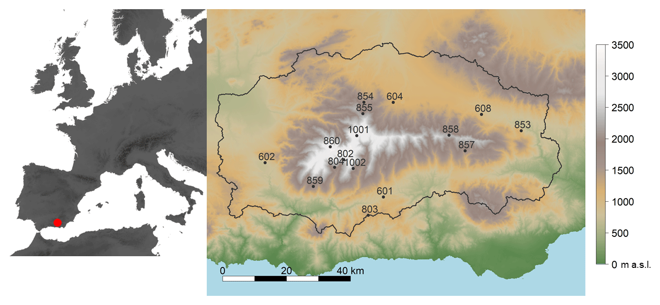
Figure 1Location of the study site in southern Spain (left). Digital elevation model (DEM) and weather stations in Sierra Nevada (SN) (right). The numbers correspond to the station codes.
The Sierra Nevada mountain range (SN) is located 35 km north of the Mediterranean Sea (Fig. 1) and constitutes a mountainous area of the Natura 2000 network. Elevations rise up from 262 to 3479 m a.s.l. in a 4583.72 km2 area that runs parallel to the sea. High altitudinal gradients are representative of the area, with variation in elevation of about 3400 m in less than 40 km of horizontal distance and a mountain climate in the summits surrounded by Mediterranean climate in the lower areas. Thus, the interaction of such conditions creates a strong heterogeneity in terms of soil types, landforms, and vegetation species that determine a complex hydrological response in the area and many endemic species (Heywood, 1995; Blanca et al., 1998; Anderson et al., 2011). The rainfall regime is highly variable, even in consecutive years, with annual cumulative values in the period (1960–2000) that range between 200 mm in dry years to 1000 mm in wet years, with an average value of 510 mm (Pérez-Palazón et al., 2015). The temperature regime is also heterogeneous, with values of 26, 12.5, and 0.4 ∘C for maximum, mean, and minimum daily temperature in the same period.
The snow presence becomes relevant from November above 2000 m a.s.l. and extends up to spring with conditions that make the activity of a major ski resort in the area possible. However, in some winters, mild episodes can be found in January and February that melt most of the snow much earlier than the mean end of the snow season in the area (Herrero et al., 2009; Herrero and Polo, 2012; Pimentel et al., 2013). Because of its singular characteristics and fragile environment, Sierra Nevada receives international recognition as a biosphere reserve (1986), a national park (1999), an important bird area (2003), a special area of conservation (2012) and one of the international global change observatories in mountain areas. These environmental protection figures together with the different and numerous members involved in the management of such a unique area have determined the strong effort in data collection in the last years to advance the knowledge of the different aspects that determine the dynamics of this natural system. Moreover, global warming impacts threaten the environmental values of this system but also the associated ecosystem services and social and economic activities due to the estimated shift of the snowfall regime (Pérez-Palazón et al., 2018).
3.1 Input data
A digital elevation model (DEM) with 30 m spatial resolution and 1 m vertical precision was used in this study (Fig. 1). The DEM was provided by the Andalusian regional administration, and it was generated by digital stereo correlation of aerial photographs of the Spanish National Plan for Aerial Orthophotography. The DEM is used to calculate the slope, aspect, sky view factor, and terrain configuration maps that are used in the modeling process (Dozier and Frew, 1990).
Table 1Information of the weather stations included in this study: elevation, z (m a.s.l.); code; data length, as initial and final dates of the time series; number of initially available daily records, No (days); number of available daily records after the quality check, N (days); rate of days for cloudy, NCI<0.3 (%), partially cloudy, (%), and clear-sky conditions, NCI>0.6 (%); and maximum, Rgo_max (MJ m−2 d−1), mean, Rgo_mean (MJ m−2 d−1), and minimum, Rgo_min (MJ m−2 d−1), daily global radiation observed values. The selected descriptors for sky conditions and global radiation correspond to registered data after quality check.
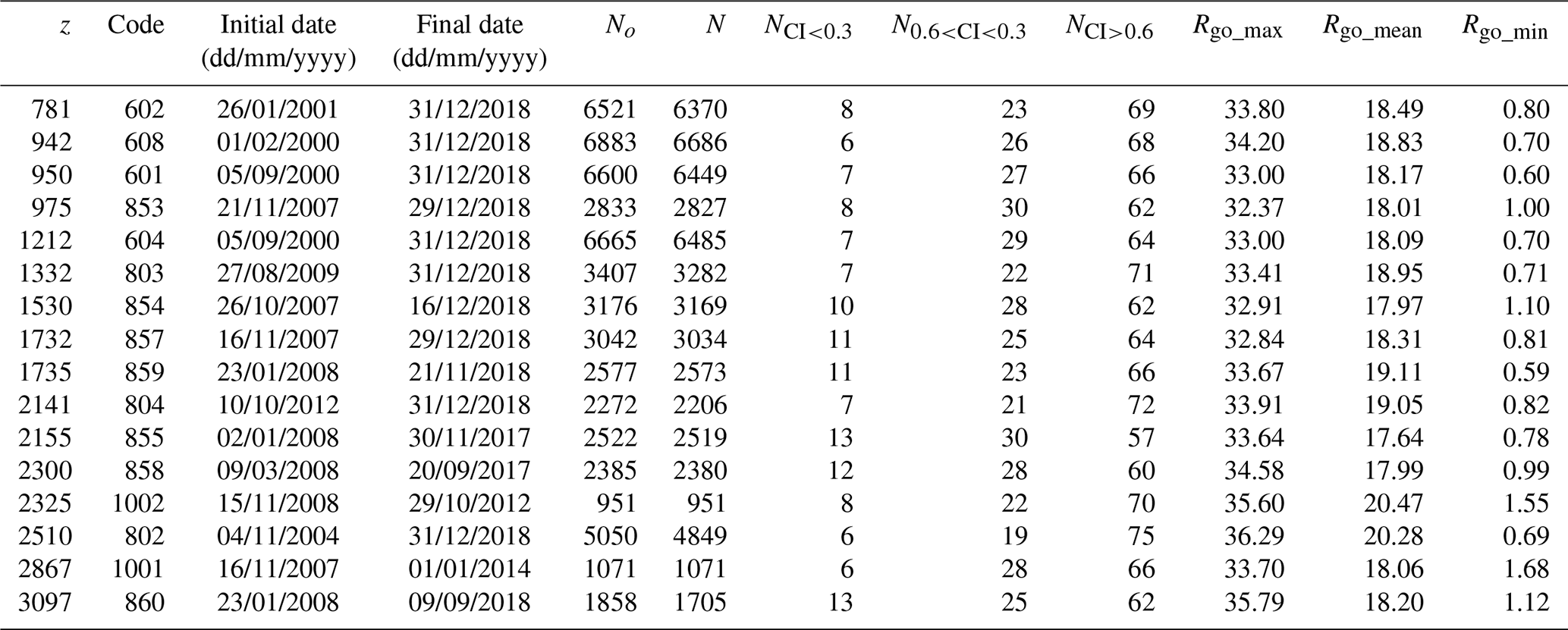
Meteorological input data are the longest available in situ daily global radiation (Rgo) of 16 weather stations over the area (Fig. 1 and Table 1). The extent of the records in all weather stations (No in Table 1) was considered long enough to carry out the evaluation process dating from February 2000 for the oldest station (608 in Table 1). Twelve out of the 16 weather stations are located above 1500 m a.s.l. and 7 of them above 2000 m a.s.l. (Fig. 1). The stations belong to four different organizations: the Department of Agriculture, Fisheries and Environment of the Andalusian Government (601–608 in Table 1), the Water and Environment Agency (1001 and 1002 in Table 1), the National Parks Organization (853–860 in Table 1), and the Guadalfeo Monitoring Network (802–804 in Table 1) described in Polo et al. (2019). Pyranometers used to collect the data were of different natures but all of them with a characteristic range of around 0.35–1.1 µm: Skye SP1110 (stations 601, 602, 604, and 608), Kipp & Zonen SP-Lite pyranometer (station 802), Hukseflux LP02 (station 803), Hukseflux NR01 (stations 1001, 1002, and 804), and Kipp & Zonen CNR1 net radiometer (stations 853, 854, 855, 857, 858, 859, and 860).
In order to generate the complete global radiation data series for the whole time span (1 February 2000–31 December 2018), we first apply a quality control check to the recorded data at the weather stations.
3.2 Data quality control
Numerous studies on quality control of measured solar radiation data can be found in the literature (Geiger et al., 2002; Younes et al., 2005; Moradi, 2009; Journée and Bertrand, 2011). Compared to other meteorological variables, solar radiation measurement is more prone to errors (Moradi, 2009). Younes et al. (2005) state two main sources of errors related to in situ measurement of solar radiation: those related to equipment and uncertainty and operational errors. Thus, prior to any computation two basic screenings were applied to recorded daily global radiation data to discard suspicious records associated with equipment and operational errors (Younes et al., 2005).
-
Observed daily global radiation (Rgo) must be between the daily extraterrestrial radiation (Rext) and a minimum 3 % of Rext (Geiger et al., 2002; Moradi, 2009).
-
Observed daily global radiation (Rgo) must be lower than the clear daily global radiation (Rgcs) observed under a highly transparent clear sky (Wu et al., 2007). Rgcs values were calculated with the model developed by Ineichen and Perez (2002) and the parameterization of Kasten and Young (1989) for the air mass. More detail regarding the equation as well as its parameters can be found in Aguilar et al. (2010).
The excluded values from these tests did not reach 1 % of the data at any weather station.
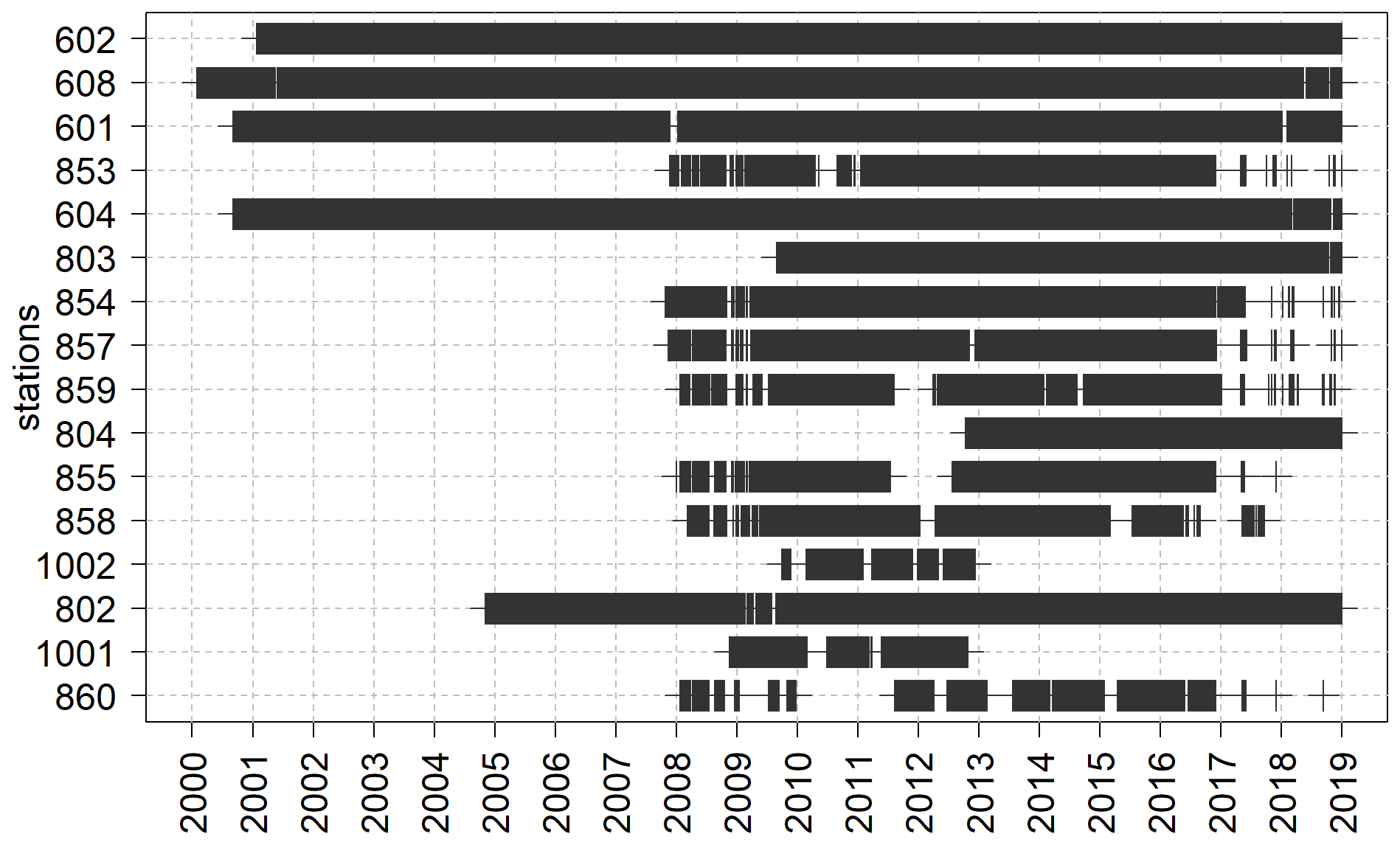
Figure 2Data availability in the analyzed period (1 February 2000–31 December 2018) for each weather station. Stations are sorted by increasing altitude from the top to the bottom row.
A third quality control screening was applied following Younes et al. (2005) to detect erroneous data due to operational errors related with particularities of weather stations in high altitudes (e.g., shadows, impacts of snow, mechanical failures, etc.). They suggest a semi-automatic procedure that allows the creation of an expectancy envelope in the clearness index (CI) diffuse-to-global-irradiance ratio (k) domain to reject data too obviously erroneous. The CI data range is divided into bands of equal width, within which the mean and standard deviation of the k values, μk and σk, are calculated. The top and bottom boundary shapes are identified by fitting two polynomials through the points μk±bσk limited between 0 and 1 to respect the physical range of the CI. In this study b values between 2 and 3 were applied to limit both the rejection of good data and the acceptance of erroneous data to small percentages.
The CI was calculated with the observed data at each weather station. However, no measurements of daily diffuse radiation, Rd, were available. Thus, the model proposed by Aguilar et al. (2010) was applied to generate daily diffuse radiation (Rdp) at each weather station without considering the observed global data at such station. Obviously, this assumption depends on the validity of the model as well as on the quality of Rgo datasets at the remaining weather stations. However, under the common lack of diffuse solar radiation measurements like the present one, modeling them can be an alternative (e.g., Yang et al., 2020) to reject erroneous Rg observations. This approach was proposed once the model had already been validated in a previous study (Aguilar et al., 2010) but keeping in mind the intrinsic limitations and assumptions previously stated.
After this quality test, the percentage of excluded values did not reach 10 % at any weather station, with a mean value close to 2 % when the whole set of stations was considered. Table 1 shows selected descriptors of the datasets at each station in this study after all the quality check process and Fig. 2 shows the chronogram of the final input data availability per station (N in Table 1) used in this study.
3.3 Generation of global radiation maps
The GIS-based solar radiation model proposed by Aguilar et al. (2010) that was previously implemented and validated in a small subwatershed located in the southwest of Sierra Nevada (Fig. 1) was extended to the whole area in this study. For validation purposes, data registered at weather stations are considered to represent the average values of the 30 m cell of the DEM on which they are located (Batllés et al., 2008; Martínez-Durbán et al., 2009).
The main equations and flowchart of the model are shown in Appendix A. The complete explanation of the algorithms as well as the justification of the assumptions of the model can be found in detail in Aguilar et al. (2010).
The model was developed to be run using limited data but considering the agents that constitute the main sources of the spatial and temporal variability of solar radiation. Results generated by the model include hourly maps of diffuse, beam, and reflected solar radiation values with minimum input data requirements as only topographic data, albedo estimations, and measured daily global radiation records (Rgo) at least at one weather station are required. As for the daily global radiation registers, even when they are missing, their estimation from other more readily available meteorological data could always be a choice from the literature (Hargreaves and Samani, 1982; Bristow and Campbell, 1984; Allen, 1997; Bechini et al., 2000; Winslow et al., 2001; Donatelli et al., 2003, 2006; Yang and Koike, 2005; Diodato and Bellocchi, 2007; Wu et al., 2007; Ruiz-Arias et al., 2011; J. Liu et al., 2012; El Ouderni et al., 2013; Mullen et al., 2013).
The generation of global radiation maps with the model applied (Aguilar et al., 2010) requires a proper characterization of the spatiotemporal patterns of albedo in the study site. A total of 240 cloud-free Landsat images available for the study period from Landsat 5 TM (49 images), Landsat 7 ETM+ (141 images), and Landsat 8 OLI (50 images) with a 30 m spatial resolution were used. Figure 3 shows the specific dates and sensors of the 240 images analyzed in this study. All images were first properly corrected, and their reflectivity values were computed (Pimentel et al., 2014). Albedo was then derived for each image following the same procedure applied in Aguilar et al. (2010), which is based on the methodology described by Brest and Goward (1987), and linearly interpolated on a daily timescale for the whole study period.
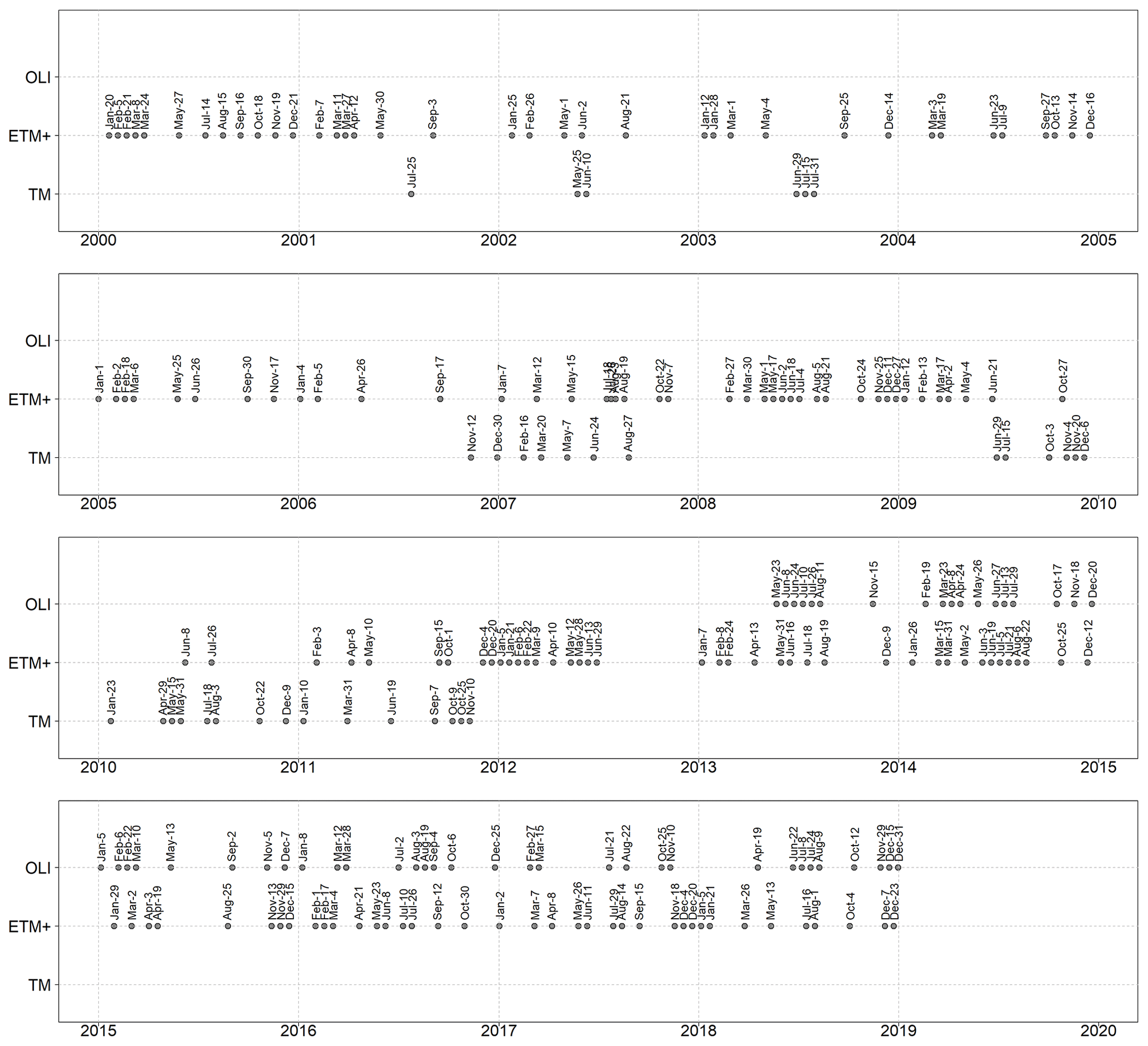
Figure 3Dates and sensors of each Landsat image analyzed in the study period (1 February 2000–31 December 2018).
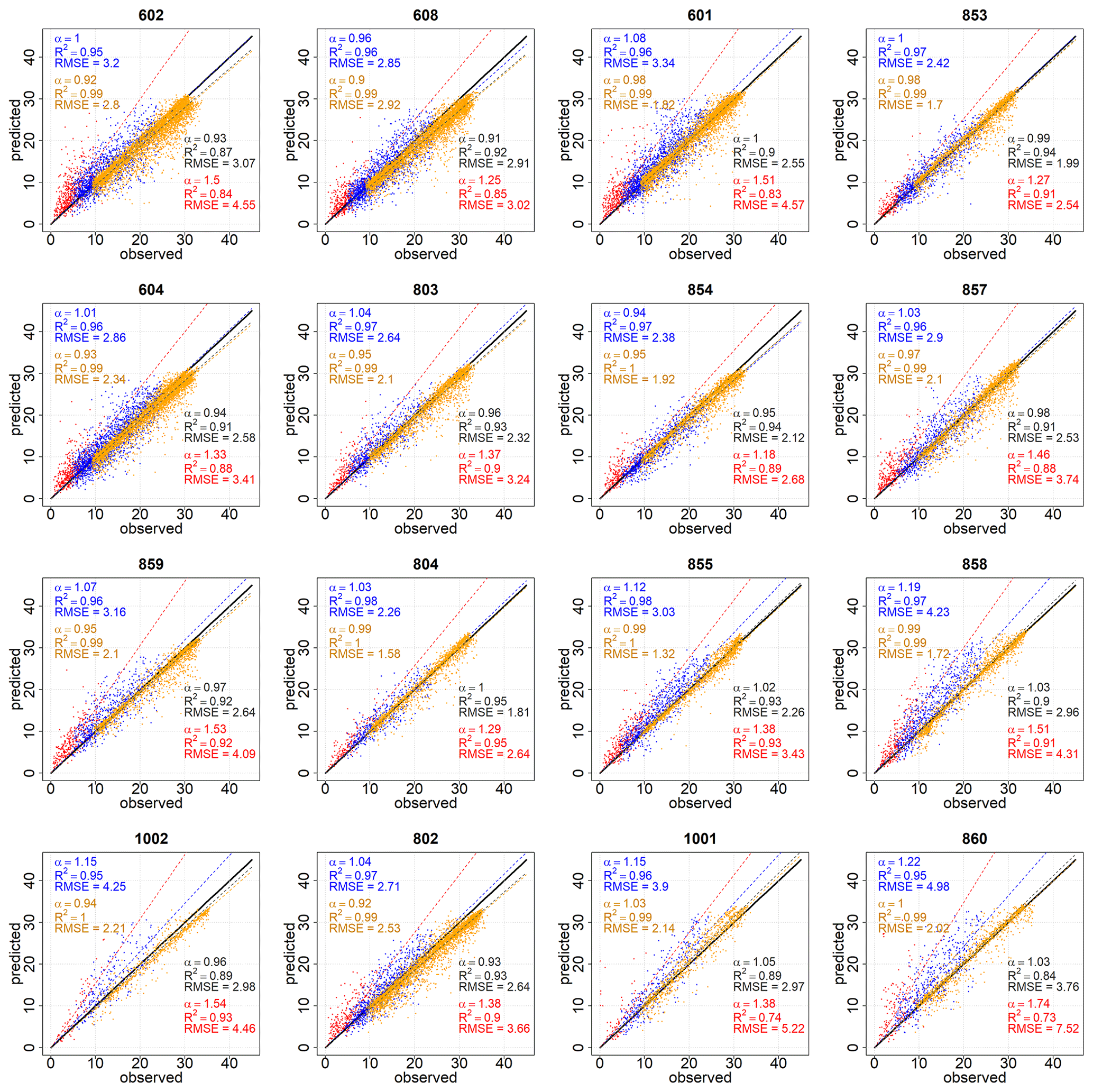
Figure 4Cross-validation analysis. Linear fits of daily predicted vs. observed Rg (MJ m−2 d−1) at each of the selected stations for the global data (black) and cloudy (CI < 0.3 – red), partly cloudy (0.3 < CI < 0.6 – blue), and clear-sky (CI > 0.6 – orange) days. Stations are sorted by increasing altitude from left to right and from the top to the bottom row.
3.4 Cross validation at weather stations
Once daily global radiation estimates were generated by the model a cross validation was applied at each weather station on the daily scale. This was carried out on a leave-one-out process; i.e., data from a weather station were removed from the input dataset to the model, and predicted values (Rgp) at that weather station were then compared to observed data (Rgo).
Different indicators were computed to quantitatively evaluate the performance of the model (Muneer et al., 2007):
-
The root mean square error (RMSE) (Eq. 1), where Rgp and Rgo are the predicted and observed daily global radiation (MJ m−2 d−1), respectively, and N is the number of observed daily data. It measures the difference between values predicted by the model and those which were observed.
-
The deviation from the 1:1 line of observed vs. predicted daily solar radiation values. Linear fits forced through the origin were obtained (Eq. 2), and the slopes (α in Eq. 2) are desired to be equal to 1. The coefficient of determination, R2, as the ratio of the explained variation to the total variation, was also computed.
The RMSE values and linear fits were obtained for the whole dataset at each weather station and also for different cloudiness levels to consider different atmospheric states that may condition the performance of the model according to previous studies (Batllés et al., 2008; Martínez-Durbán et al., 2009; Ruiz-Arias et al., 2009). Based on the cloudiness, three types of weather conditions were analyzed: cloudy days (CI < 0.3), partly cloudy days (0.3≤ CI < 0.6), and clear-sky days or cloudless days (CI ≥ 0.6).
The cross-validation analysis was also carried out with deseasonalized daily data to remove the expected intra-annual course of global radiation data. The deseasonalization of the daily series was carried out applying a stable seasonal filter (Brockwell and Davis, 2002) as already done in a previous study with other hydrometeorological datasets (Aguilar et al., 2017). In addition, as the reliability of solar radiation estimates is conditioned by the availability of recorded data, the cross-validation analysis for the whole study period was also computed with limited data. Thus, global radiation estimated was generated with only the four stations (601, 602, 604 and 608 in Fig. 1) with the longest records (Fig. 2) as inputs to the model. Results are shown in Appendix B.
Finally, to contrast the modeling scheme applied, another well-known GIS-based solar radiation model, Solar Analyst (SA) (Fu and Rich, 2000b), was also applied in the study site. Error values in the approximation to observed data and linear fits obtained in SN are shown in Appendix C.
The cross-validation assessment is summarized in Fig. 4. With the global datasets (in black in Fig. 4), a very close approximation of the model estimates to recorded data was obtained (mean α value of 0.98 and mean R2 values of 0.91). RMSE values varied for the different stations and ranged from 1.81 (station 804) to 3.76 (station 860) with a mean value of 2.63 MJ m−2 d−1.
When the analysis was carried out in terms of the cloudiness level, a general overestimation by the model (e.g., a mean α value of 1.41) was always seen on cloudy days (CI ≤ 0.3). In contrast, on clear-sky days (CI > 0.6) slopes were very close to 1 with a mean α value of 0.96. An intermediate behavior was found on partly cloudy days (0.3 < CI ≤ 0.6) when the model slightly underpredicted (e.g., stations 854 and 608) or overpredicted depending on the weather station. As for RMSE values, the lowest values were always found for clear-sky days, when the cloud influence is minimal and the attenuation is mostly explained by changes in the atmospheric transmittance, followed by partly cloudy days with mean values of 2.07 and 3.07 MJ m−2 d−1, respectively. The highest RMSE values were always found on cloudy days with mean values of 3.70 MJ m−2 d−1. The high proportion of clear-sky days (65 %) and the low RMSE values on these days (2.07 MJ m−2 d−1) revealed the general good agreement of the model estimates with observed data. This is especially important in semiarid environments, where energy-limited hydrological processes (e.g., soil moisture depletion, evaporation, or snowmelt) are more relevant on clear-sky days, and they must be carefully computed in water and energy balance modeling, irrigation scheduling, etc. (Chen et al., 1999; Mamassis et al., 2012).
There is no clear pattern in the errors obtained with the elevation of the stations. The goodness of the model estimates was more affected by the interaction of the different characteristics of the weather station (e.g., slope, aspect, surrounding terrain configuration, orographic effects in the vertical development of clouds, etc.) than by the height of the station itself.
With the deseasonalized time series (Fig. B1), differences were reduced among the different cloudiness levels. The most remarkable change was a significant improvement in the estimates of cloudy days in every station when the range of RMSE values shifted from 2.54–7.52 (in red in Fig. 4) to 1.72–5.16 MJ m−2 d−1 (in red in Fig. B1). Also, the range of the slopes significantly narrowed from 1.18–1.74 (red α values in Fig. 4) to 0.92–1.09 (red α values in Fig. B1). Thus, the comparison with deseasonalized data showed a higher accuracy of the model than the one obtained with the original datasets (Fig. 4).
The comparison with limited input datasets shown in Fig. B2 confirmed the lower reliability of global radiation estimates in the first 5 years when datasets recorded at only four stations (601, 602, 604 and 608 in Fig. 1) were available in SN. Here, higher-elevation stations are subjected to a slightly greater overestimation of solar radiation (1.34–2.04 in red in Fig. B2), especially during cloudy conditions when the RMSE values increased to 3.62–8.45 MJ m−2 d−1 (in red in Fig. B2).
The application of Solar Analyst (Table C1) revealed in general worse approximations to observed data than those shown in Fig. 4, with mean R2 values of 0.66 and RMSE values ranging from 3.59 (station 853) to 5.11 (station 859) with the global datasets.
The errors obtained in Fig. 4 were within the order of magnitude of those found in previous studies in other mountainous areas (Yang et al., 2006; 2010; Zhang et al., 2020) and slightly improved those previously obtained on a small subarea (10 × 5 km2) in the northeastern side of SN. Here, Tovar-Pescador et al. (2006) analyzed the application of SA in clear-sky days with 168 daily global radiation values in the dataset from 14 weather stations located between 1091 and 1659 m a.s.l. They obtained R2 values of 0.75, similar to the value here obtained with SA estimates in the whole SN area (0.77 in Table B1) but lower than the R2 equal to 0.99 obtained with the model (in orange in Fig. 3). Then, Batllés et al. (2008) in another application of SA in the same area with a 2-year daily dataset obtained the best performances for clear-sky days. RMSE values obtained in clear-sky days in the present study, of 11.1 % (2.07 MJ m−2 d−1), were the same as those obtained by Batllés et al. (2008) for clear-sky days (11 %). Later, Ruiz-Arias et al. (2009) evaluated the application of four different GIS-based solar radiation models with 523 daily global radiation values in the dataset at the same study site. RMSE values for the global dataset ranged between 1.99 and 7.28 MJ m−2 d−1 depending on the model.
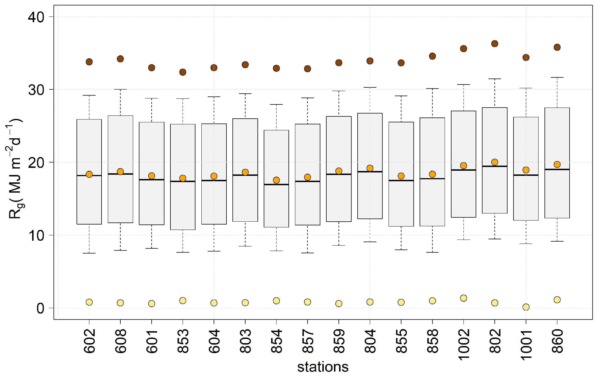
Figure 5Statistical distribution of daily Rg (MJ m−2 d−1) time series at each of the selected stations over the study area. The box shows 50 % of the data, delimited by Q1 (lower) and Q3 (upper), the solid line represents the median, and whiskers show 10th and 90th percentiles. Brown, orange, and yellow dots represent daily maximum, mean, and minimum time series values. Stations are sorted by increasing altitude from left to right.
The order of magnitude of the errors (Fig. 4) and its comparison with those obtained with more computationally and data-demanding GIS-based models in previous studies led us to conclude that the model is the best choice to generate global radiation data series in SN.
Therefore, once the model was validated in the study site, daily Rg maps were generated and aggregated at the monthly and annual scales.
Daily, monthly, and annual Rg datasets in SN are analyzed in this section at two spatial scales. First, the results at the weather station scale are presented. Thus, possible relationships between altitude and/or location of the weather station with the different Rg statistics and how this relation changes with the temporal scale of analysis can be assessed. Then, the Rg maps that can be downloaded as specified in Sect. 5 are analyzed.
4.1 Daily time series of global radiation in Sierra Nevada
Figure 5 shows the statistical distribution of the daily Rg at each weather station ordered by increasing altitude and illustrates several questions. First, there is a very similar interquartile range among stations. Second, there are greater variations in the maximum daily Rg among the different stations with a mean value of 34.0 MJ m−2 d−1. Third, even though a slight increase with altitude can be shown in the high extreme statistics of the daily Rg values (e.g., in the maximum or in the 90th percentile), there is not a clear trend. Therefore, other factors such as orientation, proximity to the sea, or the terrain configuration in the surrounding terrain as suggested by Batllés et al. (2008) constitute relevant features in the study site.
Figure 6 shows an example of the spatial distribution in three representative days of cloudy, partially cloudy, and clear-sky conditions. Here the spatial distribution is clearly influenced by the topography of SN, especially in the clear-sky day.
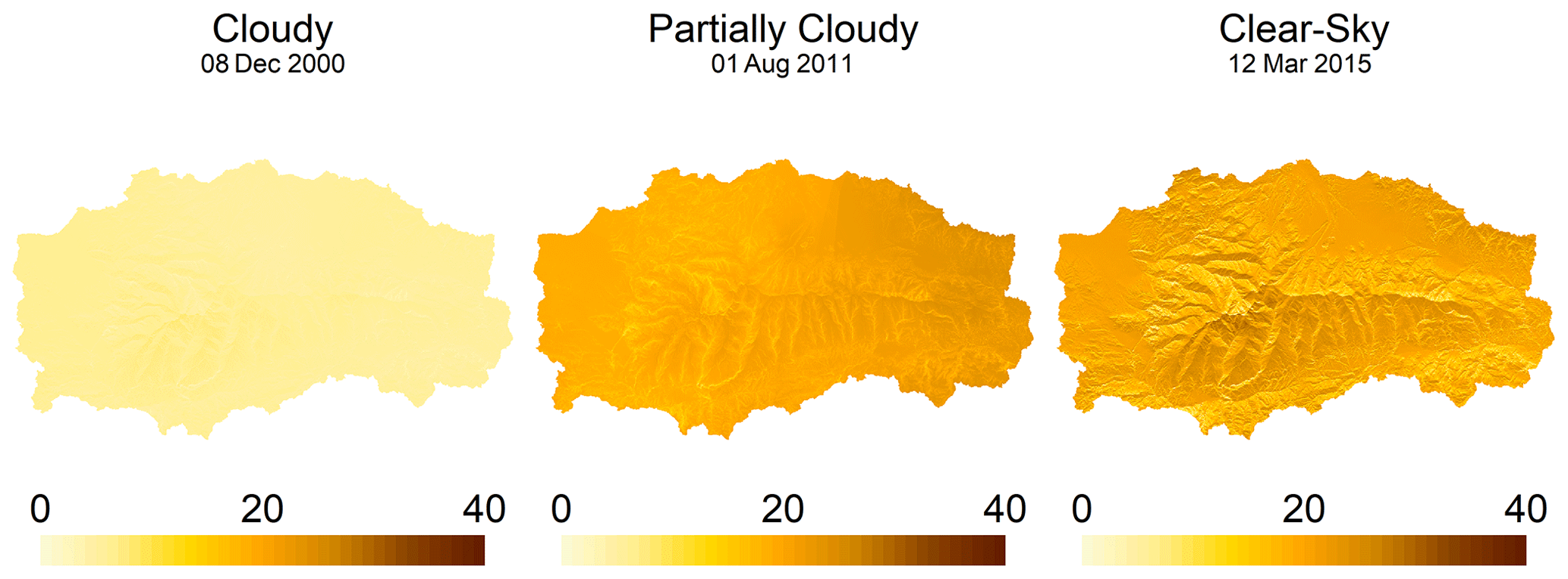
Figure 6Daily Rg (MJ m−2 d−1) in SN for three selected days that represent the three levels of cloudiness considered in this study: cloudy, partially cloudy, and clear sky.

Figure 7Statistical distribution of monthly Rg (MJ m−2 per month) time series at each of the selected stations over the study area. The box shows 50 % of the data, delimited by Q1 (lower) and Q3 (upper); the solid line represents the median; and whiskers show the 10th and 90th percentiles. Brown, orange, and yellow dots represent monthly maximum, mean, and minimum time series values. Stations are sorted by increasing altitude from left to right and from the top to the bottom row.
4.2 Monthly time series of global radiation in Sierra Nevada
The statistical distribution of monthly Rg per weather station (Fig. 7) shows that in every station (i) July and December constitute the months with the highest and the lowest values of Rg, respectively; (ii) there is a quite linear increase in the monthly Rg values from January to July and a sudden drop in August with a slightly convex evolution till December; and (iii) the interquartile range is significantly higher in the spring and fall than in the summer and winter months.
The increase in the high extreme statistics of radiation with the altitude of the weather station becomes more apparent at the monthly scale (Fig. 7) than at the daily scale (Fig. 5) previously analyzed. Thus, maximum values of around 1000 MJ m−2 per month are reached in July in the highest stations (e.g., 1002, 802, 1001, and 860 in Fig. 7), whereas this value decreases to around 910 MJ m−2 per month in the four lowest stations except for station 608.
Monthly Rg maps show significant spatial differences of up to 200 MJ m−2 per month in both the mean monthly values (Fig. 8) that clearly follow the terrain configuration, with summits and valleys receiving high and low solar radiation values, respectively. For example, the area in the north of SN that is highly shadowed by the highest peaks in the Iberian Peninsula (Mulhacen and Veleta with 3482 and 3396 m a.s.l., respectively) is easily visible, with the lowest relative levels of insolation received within SN especially in the summer months (June, July, and August in Fig. 8).
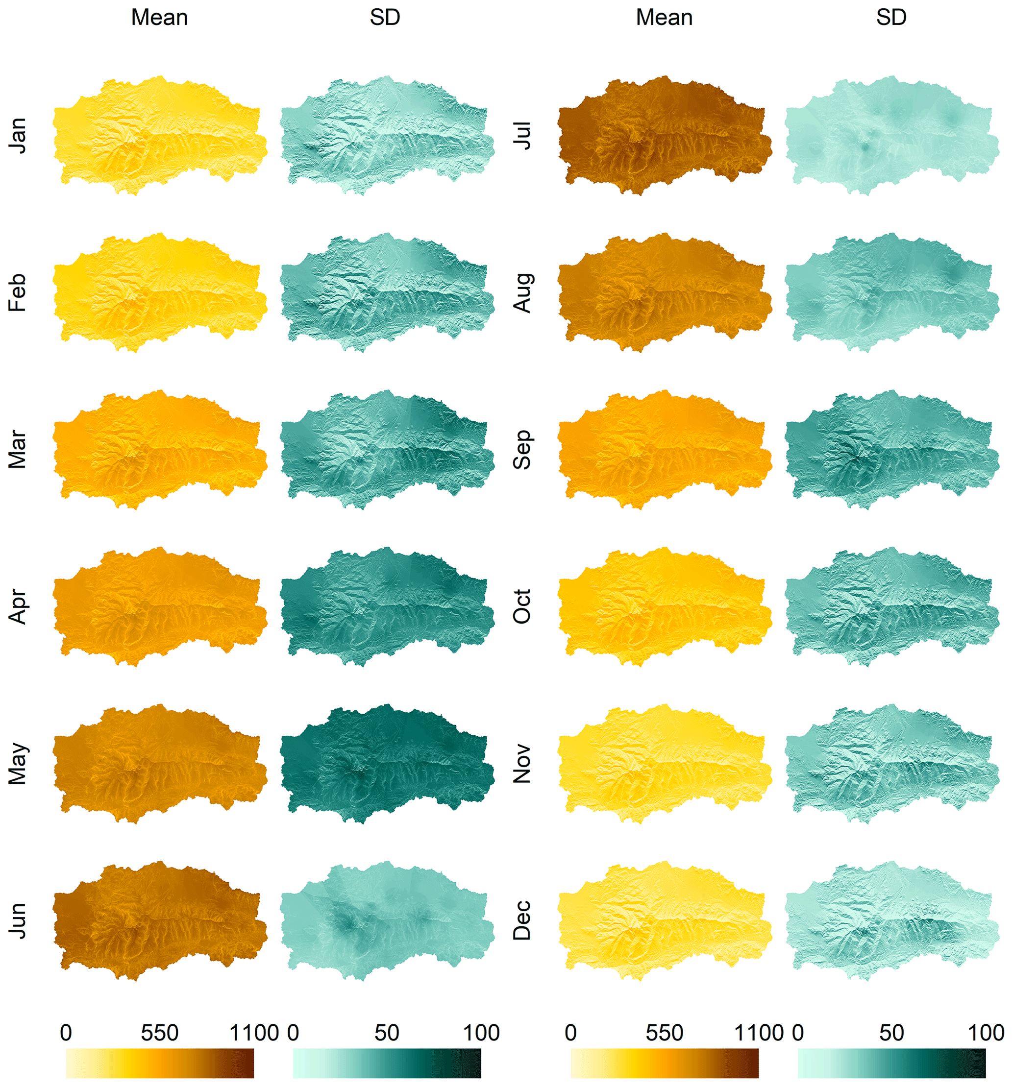
Figure 8Monthly average and standard deviation of Rg (MJ m−2 per month) in the study period (2000–2018) in SN.
Both maps of the monthly mean and standard deviation of Rg (Fig. 8) and the statistical distribution of the monthly Rg in the study site (Fig. 9) show the same behavior as the one obtained at the weather stations regarding (i) July and December as the months with the highest and lowest values of Rg received in SN and (ii) the highest scatter in the monthly Rg values in the spring and fall months.
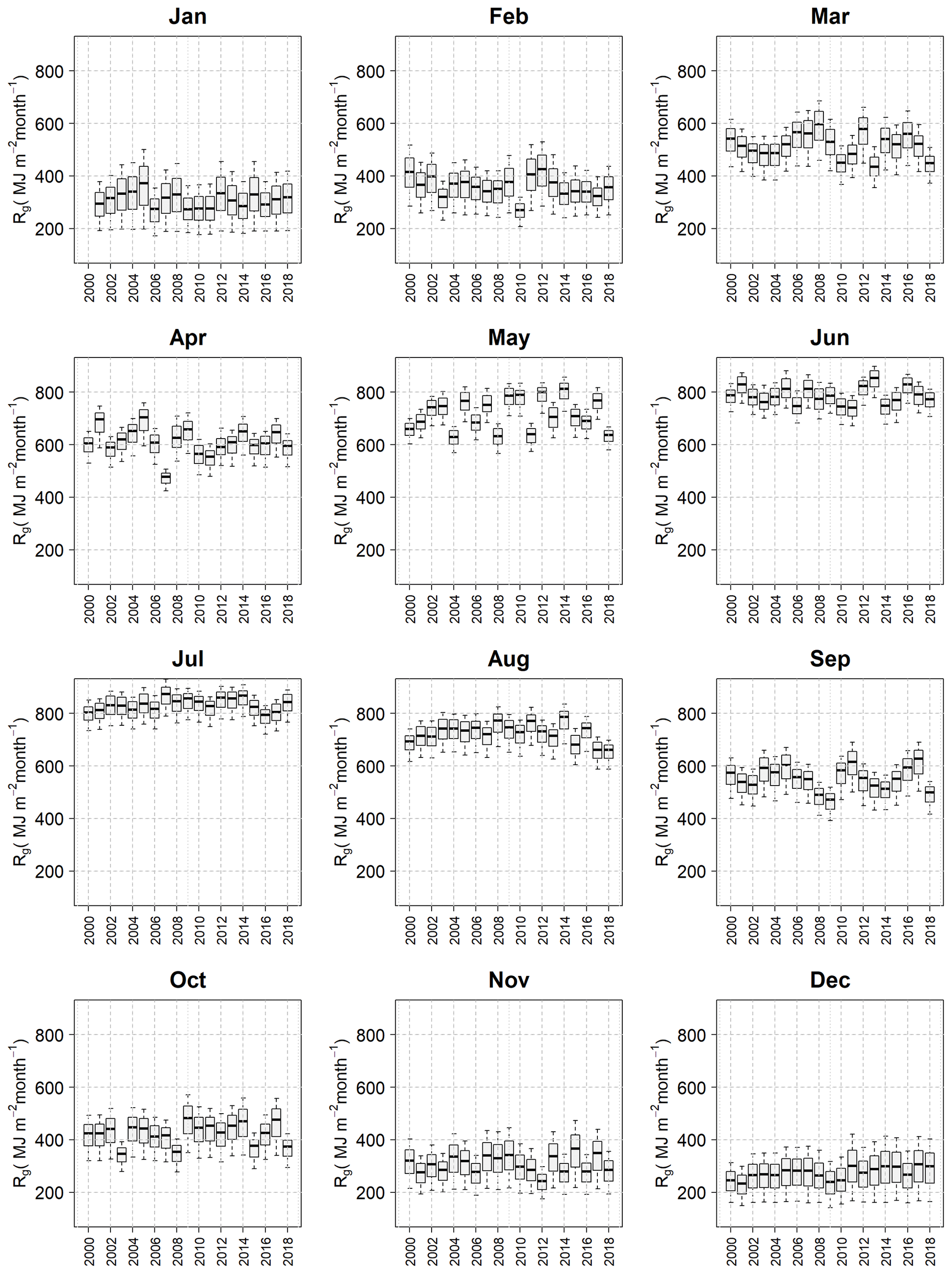
Figure 9Statistical distribution of the monthly Rg (MJ m−2 per month) values throughout the study area. Whisker boxes represent the 10th, 25th, 50th, 75th, and 90th percentiles of each monthly map per year.
For the study period (2000–2018), there is a great heterogeneity in the statistical distribution of the monthly Rg in the study site (Fig. 9), especially in the incoming radiation along the months of the wet season (October–May). In this way, in the most insolated years in the study period (2005 and 2012), significantly higher monthly radiation values were found in certain months of the springtime (March and May 2012 and April 2005). In those months, the higher-than-usual rate of clear-sky over cloudy days finally determines the annual differences in the incoming global radiation in SN.
When considering the temporal evolution of the distribution of Rg within the monthly maps in SN (Fig. 10), certain interannual differences can be observed along the study period, such as the existence of certain months in spring with unexpected low monthly radiation values (e.g., 2001, 2004, 2007 and 2008) or two relative maximum monthly Rg values (e.g., 2009, 2010, and 2014). Moreover, Fig. 10 shows a higher scatter in the monthly maximum (June–August) and minimum (November–January) Rg values in SN than when the analysis is carried out at each weather station (Fig. 7).
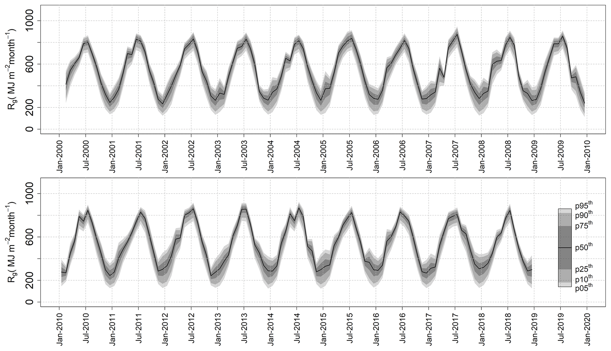
Figure 10Evolution of the statistical distribution of monthly Rg (MJ m−2 per month) in the study period (2001–2018) throughout the study area. Grayscale colors represent the following percentiles: 5th, 10th, 25th, 50th, 75th, 90th, and 95th.
4.3 Annual times series of global radiation in Sierra Nevada
Unlike at the daily scale (Fig. 5), a great variability among the different weather stations in terms of the global radiation received at the annual temporal scale is found (Fig. 11). Thus, we find minimum annual Rg values from 5920 MJ m−2 yr−1 in station 854 to around 6750 MJ m−2 yr−1 in station 1002. This difference is even bigger in the maximum annual Rg values from 6700 to 7720 MJ m−2 yr−1 in stations 854 and 802, respectively, and is also shown in the interquartile range.
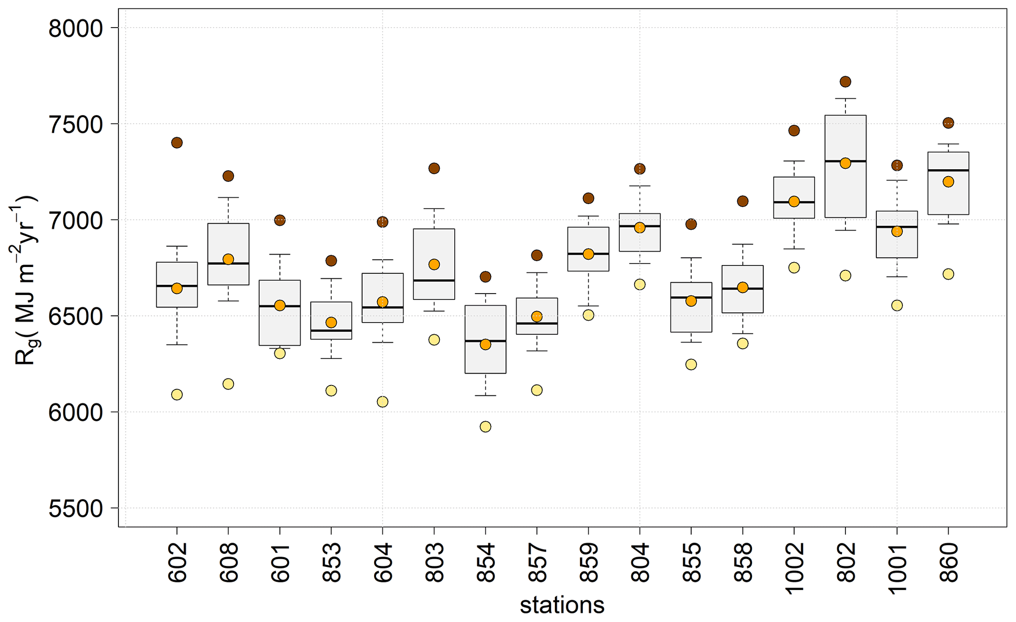
Figure 11Statistical distribution of annual Rg (MJ m−2 yr−1) time series at each of the selected stations over the study area. The box shows 50 % of the data, delimited by Q1 (lower) and Q3 (upper); the solid line represents the median; and whiskers show 10th and 90th percentiles. Brown, orange, and yellow dots represent annual maximum, mean, and minimum time series value. Stations are sorted by increasing altitude from left to right.
When analyzing the influence of altitude, the weather stations above 1500 m a.s.l (854, 857, 859, 804, 855, 858, 1002, 802, 1001, and 860 in Fig. 11) show their altitudinal gradient in all the statistics of the annual Rg values considered.
Annual Rg maps (Fig. 12) show the same spatial differences that follow the terrain configuration as those observed in the monthly time series (Fig. 8). For example, the area in the north of SN that is highly shadowed as previously mentioned corresponds to the area with the mean minimum annual values received in the study period, 4063 MJ m−2 yr−1, that only represents 63 % of the mean annual accumulated values in SN (6316 MJ m−2 yr−1).
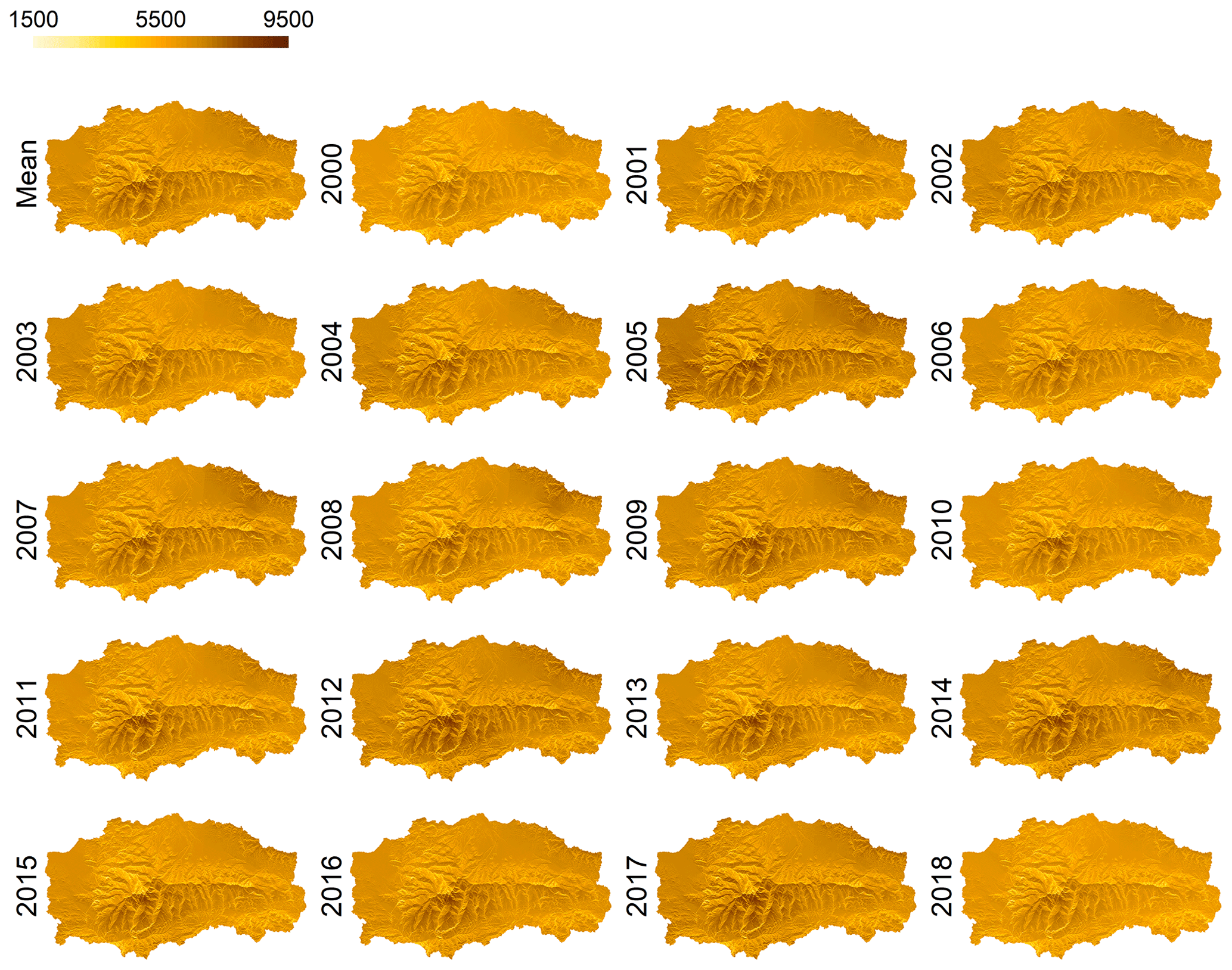
Significant interannual differences can be easily shown with differences in the mean annual Rg value in the study area of up to 800 MJ m−2 yr−1 between 2005 and 2018. Such years with particularly high and low annual incoming radiation also presented higher (6800 MJ m−2 yr−1) and lower median annual Rg values (6200 MJ m−2 yr−1), respectively, than the annual median for the whole study period in SN (6456 MJ m−2 yr−1) (Fig. 13). These results agree with the annual irradiation map obtained by Batllés et al. (2008) in the northeastern part of SN. They reported maximum and minimum annual values of 7516 and 2342 MJ m−2 yr−1 on the summits and in deep valleys, respectively, and thus concluded that irradiation levels were more related to topographic characteristics than to altitude.
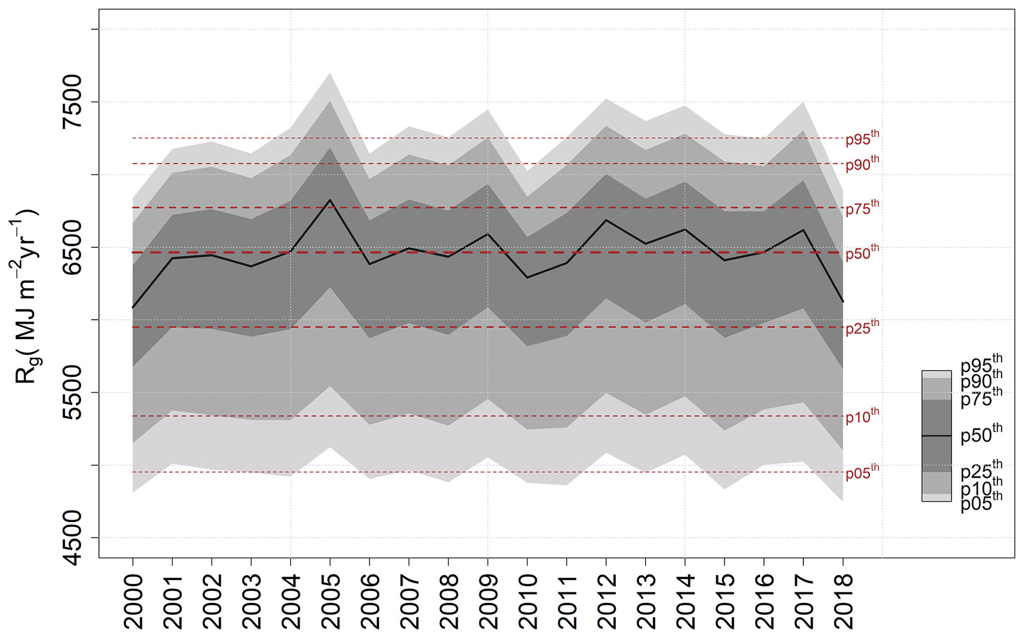
Figure 13Evolution of the statistical distribution of annual Rg (MJ m−2 yr−1) in the study period (2001–2018) throughout the study area. Dashed lines represent the mean values of the percentiles analyzed.
The daily, monthly, and annual global radiation maps derived in this study can be accessed and downloaded in .ncdf format from https://doi.org/10.1594/PANGAEA.921012 (Aguilar et al., 2021). In addition, a .txt file containing the availability (code 1) or gaps (code 0) in the daily Rg observations at each weather station has been added as a Supplement to this paper. Hourly datasets were also computed in this study, but due to their large storing capacity requirements they have not been included in the data repository specified above. Thus, hourly maps can be provided for certain dates upon request to the authors. However, a validation of these hourly datasets like the one applied in the daily estimates at the weather stations has not been specifically carried out in this study. Therefore, in case hourly maps are requested to the authors, these data should be taken with caution as the only available validation in SN was carried out at one weather station (802 in Fig. 1) and for a shorter period (2004–2010) in Aguilar et al. (2010).
This study presents 19 years (2000–2018) of daily, monthly, and annual global radiation maps of high spatial resolution (30 m) in a high-mountain Mediterranean site. In these areas the common lack of weather stations in high altitudes makes it difficult to accurately assess solar radiation spatial patterns.
A GIS-based modeling scheme based on measurements or estimations of incoming daily global radiation was applied and validated in the 16 weather stations available at this unique study site. Mean RMSE values ranged from 1.81 to 3.76 MJ m−2 d−1, depending on the weather station. The best estimations were always obtained on clear-sky days, when mean RMSE values decreased to 2.07 MJ m−2 d−1. The largest errors were obtained on cloudy days, which constitute on average 10 % of the daily datasets, and, therefore, future research should be conducted in order to improve the estimations in these situations, keeping the minimum input data requirement (daily global radiation data) advantage of the model. However, the high proportion (65 %) of clear-sky days, and the low RMSE values on those days, allow one to conclude that there is a good agreement between the model estimates and observed data in the study site.
Spatial differences of around 2000 MJ m−2 yr−1 were found within each year analyzed. In addition, significant differences were easily shown between the years in mean incoming values of up to 800 MJ m−2 yr−1. Those differences were mostly due to the variability in the incoming radiation at the wet season (October–May), with higher rates of clear-sky days in the most insolated years (e.g., 2005).
Thus, we can affirm that the modeling scheme here applied is an efficient option in semiarid mountainous areas, where daily global radiation datasets constitute the only source of solar radiation data.
Time series of these surface global radiation datasets can be used to analyze interannual and seasonal variation characteristics of the global radiation received in SN with high spatial detail (30 m). The availability of long global radiation datasets allows us to capture the annual variability within each cycle of the sun activity, as reported in the literature (Scaffetta and Wilson, 2013), and thus estimate its contribution to the annual variability of other climate variables in these semiarid mountainous areas.
Dense and properly maintained weather station networks in mountainous areas are rarely available. Thus, these datasets can also be used as cross-validation reference data for other global radiation distributed datasets generated in SN with different spatiotemporal interpolation techniques.
These results can also assess the order of magnitude of different sources of spatial variability (altitude/slope/aspect gradients) as well as the seasonal range of variation at different timescales and their annual variability. This estimation may provide a first estimate of the order of magnitude of uncertainty of average calculations or spatial interpolation from a scarce number of weather stations in Mediterranean and semiarid mountain areas.
The correct assessment of the solar radiation regime is crucial to correctly determine the temporal evolution of energy-limited hydrological processes such as the snow layer dynamics, soil moisture depletion, and evapotranspiration (Tomas-Burguera et al., 2019). Thus, as a key input parameter for the water and energy balance, these high-spatial-resolution solar radiation time series are useful not only for research on the snow domain and water planning in SN in the application of hydrological modeling, but also in many other applications – for example, for estimations of evapotranspiration for irrigation scheduling in the agricultural sector, for ecological and biodiversity-related studies, in the design and location of stand-alone solar energy facilities, and for outdoor recreational activities in the area that strongly rely on the hydrometeorological conditions of SN. Finally, this work contributes to feed research related to some key questions in hydrology, such as UPH 16 and UPH 5 identified by Blöschl et al. (2019).
The sequence followed by the model is summarized in Fig. A1. Computations are classified at the point scale of weather stations (Point) and the distributed scale of grids of the digital elevation model (DEM) (Distributed). The complete explanation of the algorithms and assumptions of the model can be found in detail in Aguilar et al. (2010).
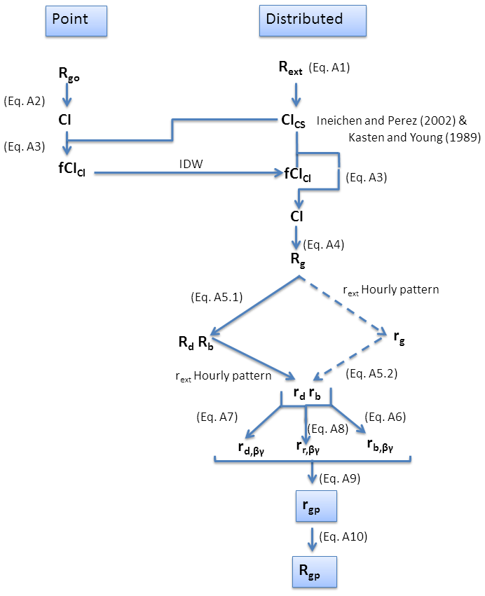
Firstly, daily extraterrestrial radiation (Rext in MJ m−2 d−1) is computed by integrating the extraterrestrial radiation incident upon a horizontal surface relative to the sun's beams from sunrise to sunset (Eq. A1).
where ISC is the solar constant (1367 W m−2), θz is the zenith angle, and Eo is the eccentricity factor. These variables were computed following the equations in Dozier et al. (1981).
Then, the daily clearness index (CI), as the ratio of observed daily global radiation (Rgo in MJ m−2 d−1) to the daily extraterrestrial radiation, is computed at each weather station (Eq. A2).
CI is expressed in terms of two factors, CICS and fCIcl. The first term represents the influence of atmosphere under clear-sky conditions over solar radiation, while the second term includes the cloudiness effects that decrease the final incoming solar radiation (Eq. A3). The approximation of Ineichen and Pérez (2002) is used to compute the global radiation under clear-sky conditions, Rgcs, and thus distributed hourly Rgcs values are obtained from the sun elevation angle, the height of the cell, the Linke turbidity factor (TL), and the atmospheric mass obtained following the parameterization of Kasten and Young (1989). Thus, hourly CICS values can be computed cell by cell, and then the mean daily distributed values are generated. Once daily CI and CICS values are known, fCIcl is obtained at each weather station from Eq. (A3) and spatially interpolated following the inverse distance weighted (IDW) method. From daily CICS and fCIcl maps, daily interpolated CI and Rg values can be obtained at the cell scale from Eqs. (A3) and (A4).
Topographic effects need to be evaluated for the different sun positions during the day, and thus hourly values of the different components need to be derived. Two different procedures are currently available in the model. The first one proposed in Aguilar et al. (2010) applies Jacovides et al. (1996) (Eq. A5a) to produce the daily diffuse (Rd in MJ m−2 d−1) and daily beam values (Rb in MJ m−2 d−1). The model finally computes hourly beam and diffuse values on horizontal surfaces (rb and rd, both in MJ m−2 h−1), from the daily amounts and following the temporal pattern of extraterrestrial hourly radiation during the day.
The second approach uses the temporal pattern of extraterrestrial hourly radiation, rext, to generate hourly global values, Rg, according to previous studies (Chen et al., 1999; Ruiz-Arias et al., 2011). Then, the hourly regressive model developed by Ruiz-Arias et al. (2010) is applied to estimate the hourly diffuse values (Eq. A5b) from the hourly CI, CIh, as the ratio of Rg to rext. This model was implemented as it has been validated over Europe and the USA using ground data from different sites, including some Spanish stations (Ruiz-Arias et al., 2010). Hourly beam values (rb) are thus obtained on a cell basis as the difference between global and diffuse hourly radiation distributed values.
First applications at the study site have shown negligible differences between both partitioning schemes. The differences with daily recorded data were insignificant in the second decimal place of error values. Thus, the results presented in this study were obtained with the original scheme of Aguilar et al. (2010) (Eq. A5a) while the authors continue working on the improvement on the partitioning scheme of the model.
Then, the topographic correction is carried out, and, depending on the component, different procedures are applied.
Hourly beam radiation on a surface of slope β and orientation γ (rb,βγ in MJ m−2 h−1) is calculated according to Eq. (A6) in terms of rb, θz, and a new corrected zenith angle for the sloping surface, θ (Iqbal, 1983). Then, the model checks the shading effects. Self-shading will occur if the angle between the normal to the surface and the solar vector is greater than 90∘. Finally, shading by nearby terrain takes place when the illumination angle is greater than the horizon angle in the same direction. The model previously obtained the horizons following the algorithms of Dozier et al. (1981) and Dozier and Frew (1990) by comparing the slopes between cells in the eight directions.
Hourly diffuse radiation on a surface of slope β and orientation γ (rd,βγ in MJ m−2 h−1) is calculated according to Eq. (A7) in terms of rd and SVF, the sky view factor that modifies the incoming radiation incident on a flat surface to consider possibly obstruction effects on a sloping surface (Dubayah, 1992). Dozier and Frew (1990) obtained an analytical expression for the estimation of the SVF in terms of the different horizons in each direction considered assuming an isotropic sky.
Finally, hourly reflected radiation on a surface of slope β and orientation γ (rr,βγ in MJ m−2 h−1) and albedo ρ is calculated according to Dozier and Frew (1990) as expressed in Eq. (A8).
Hourly global distributed radiation (rgp in MJ m−2 h−1) is obtained by addition of the three hourly components at each cell according to Eq. (A9).
Finally, daily global distributed radiation (Rgp in MJ m−2 d−1) is obtained as the summation of hourly global distributed radiation values (Eq. A10).
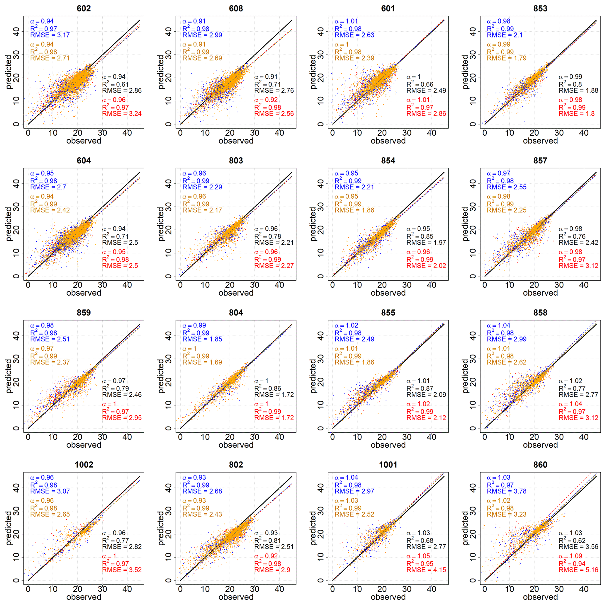
Figure B1Linear fits of daily deseasonalized predicted vs. observed Rg (MJ m−2 d−1) at each one of the selected stations for the global data (black) and cloudy (CI < 0.3 – red), partly cloudy (0.3 < CI < 0.6 – blue), and clear-sky (CI > 0.6 – orange) days. Stations are sorted by increasing altitude from left to right and from the top to the bottom row.
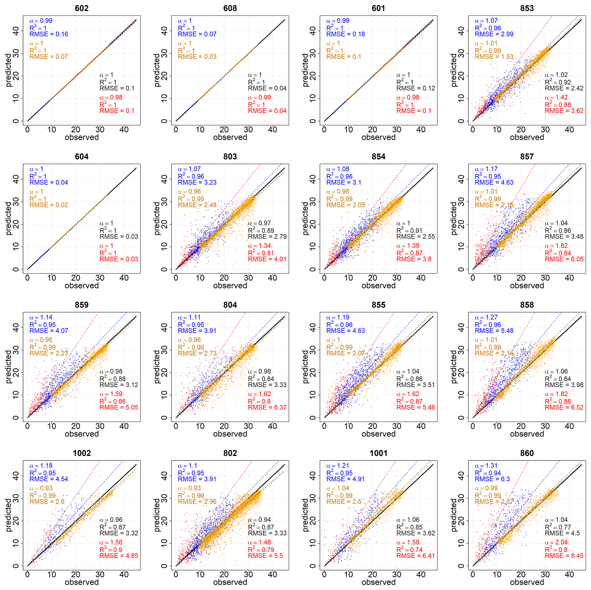
Figure B2Linear fits of daily predicted with limited input data vs. observed Rg (MJ m−2 d−1) at each one of the selected stations for the global data (black) and cloudy (CI < 0.3 – red), partly cloudy (0.3 < CI < 0.6 – blue), and clear-sky (CI > 0.6 – orange) days. Stations are sorted by increasing altitude from left to right and from the top to the bottom row.
Solar Analyst (SA) is one of the most used GIS-based solar radiation models. It calculates the insolation across a landscape or for specific locations, based on the methods developed by Fu and Rich (2000a, 2000b, 2002). The total amount of radiation is given as global radiation and depends on the latitude of the site, topography, shadow cast, and atmospheric attenuation. Global radiation is computed in SA as the sum of direct and diffuse radiation. The equations and modeling scheme can be found in detail in Fu and Rich (2000b).
Daily global radiation time series were generated in the study site with the Points Solar Radiation tool of SA at each weather station. Then a cross validation on a leave-one-out process was applied. The main inputs to the model, the diffuse fraction, k, and the atmospheric transmittivity, τ, were estimated in the study site from observed global radiation data following Batllés et al. (2008).
Table C1Model performance with Solar Analyst: slope (α) and r2 of the linear fit between daily predicted vs. observed Rg and RMSE (MJ m−2 d−1).
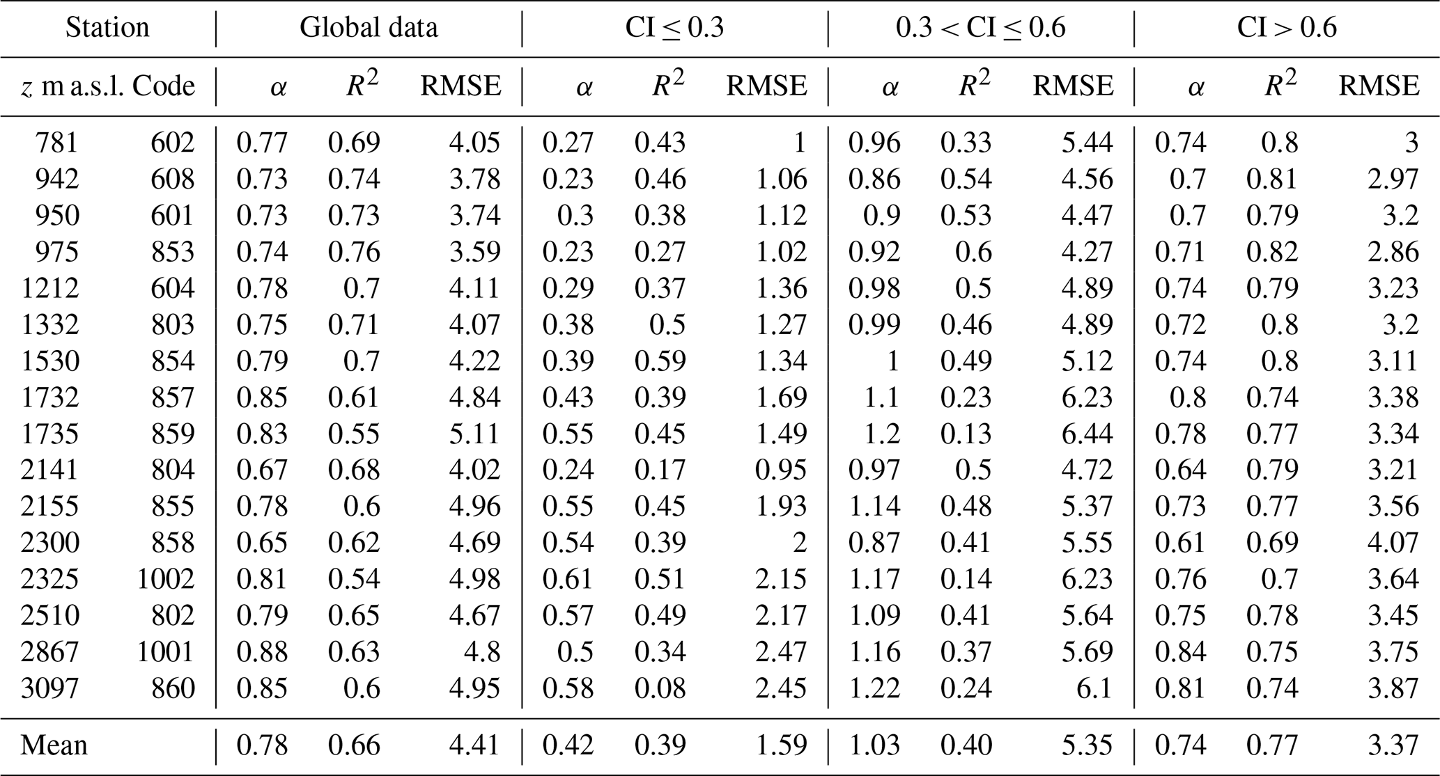
SA underestimated observed daily values with a mean α value of 0.78 in the global datasets (Table C1). In terms of the cloudiness level, a general underestimation by SA was always seen on cloudy (CI ≤ 0.3) and clear-sky days (CI > 0.6) with slopes of the fits significantly lower than 1 (mean α values of 0.42 and 0.74 respectively). In contrast, a slight overestimation with a mean α value of 1.03 was found on partly cloudy days (0.3 < CI ≤ 0.6). As for RMSE values, the lowest mean values were always found for cloudy days (1.59 MJ m−2 d−1), which are also lower than those obtained in Fig. 4 (3.70 MJ m−2 d−1). However, despite the lower RMSE values the deviation from the 1:1 linear fit in cloudy days with SA estimates was significant (mean α value of 0.42 and R2 value of 0.39 in Table C1). The highest RMSE values with SA estimates were always found on partly cloudy days with a mean value of 5.35 MJ m−2 d−1 followed by clear-sky days with a mean RMSE value of 3.37 MJ m−2 d−1, both considerably higher than those obtained in Sect. 3.4 (3.07 and 2.07 MJ m−2 d−1 respectively).
| Symbols | |
| CI: | daily clearness index |
| CICS: | daily clearness index in a cloudless atmosphere |
| CIh: | hourly clearness index |
| Eo: | eccentricity factor |
| fCIcl: | cloudiness effects factor |
| ISC: | solar constant |
| k: | diffuse-to-global-irradiance ratio |
| N CI < 0.3: | rate of days for cloudy conditions |
| N 0.3 < CI < 0.6: | rate of days for partially cloudy conditions |
| N CI > 0.6: | rate of days for clear-sky conditions |
| No: | number of initially available daily records in the study period |
| N: | number of available daily records after the quality check |
| Q1: | quartile 1 |
| Q3: | quartile 3 |
| Rb: | daily beam radiation |
| Rbp: | daily beam radiation predicted by the model |
| Rd: | daily diffuse radiation |
| Rdp: | daily diffuse radiation predicted by the model |
| Rext: | daily extraterrestrial radiation |
| Rg: | global radiation |
| Rgcs: | global radiation under clear-sky conditions |
| Rgo_max: | maximum daily global radiation observed value |
| Rgo_mean: | mean daily global radiation observed value |
| Rgo_min: | minimum daily global radiation observed value |
| Rgp: | daily global radiation predicted by the model |
| rb: | hourly beam radiation on horizontal surfaces |
| rb,βγ: | hourly beam radiation on a surface of slope β and orientation γ |
| rd: | hourly diffuse radiation on horizontal surfaces |
| rd,βγ: | hourly diffuse radiation on a surface of slope β and orientation γ |
| rext: | hourly extraterrestrial radiation |
| rr,βγ: | hourly reflected radiation on a surface of slope β and orientation γ |
| Rg: | hourly global radiation on horizontal surfaces |
| rgp: | hourly global radiation predicted by the model |
| R2: | coefficient of determination |
| TL: | Linke turbidity factor |
| z: | elevation |
| Abbreviations | |
| DEM: | digital elevation model |
| IDW: | inverse distance weighted |
| RMSE: | root mean square error |
| SA: | Solar Analyst |
| SN: | Sierra Nevada mountain range |
| SVF: | sky view factor |
| UPH: | unsolved problems in hydrology |
| Greek symbols | |
| α: | slope of the fit between Rgp and Rgo |
| β: | slope |
| γ: | orientation |
| μk: | mean of the diffuse-to-global-irradiance ratio |
| ρ: | albedo |
| σk: | standard deviation of the diffuse-to-global-irradiance ratio |
| θ: | corrected zenith angle for the sloping surface |
| θz: | zenith angle |
The supplement related to this article is available online at: https://doi.org/10.5194/essd-13-1335-2021-supplement.
CA, in collaboration with MJP, conceived the research. CA processed the data, applied the quality control to the raw global radiation data, modeled global radiation datasets, and developed the cross-validation algorithms. RP processed satellite data, generated albedo maps for the study period, and prepared the final figures and the available datasets generated in the study. CA prepared the manuscript with contributions of MJP and RP; all authors discussed and revised the final text.
The authors declare that they have no conflict of interest.
This study was supported and partially funded by the Spanish Ministry of Science and Innovation (research project RTI2018-099043-B-I00, “Operability in hydrological management under snow torrentiality/drought conditions in high mountain in semiarid watersheds”) and by the Spanish Ministry of Economy and Competitiveness (research project CGL 2014-58508R, “Global monitoring system for snow areas in Mediterranean regions: trends analysis and implications for water resource management in Sierra Nevada”; research project CGL 2011-25632, “Snow dynamics in Mediterranean regions and its modelling at different scales. Implication for water management”). Moreover, the present work was partially developed within the framework of the Panta Rhei Research Initiative of the International Association of Hydrological Sciences (IAHS) (working groups Water and energy fluxes in a changing environment and Mountain Hydrology). Rafael Pimentel acknowledges funding by the Modality 5.2 of the Programa Propio-2018 of the University of Cordoba and the Juan de la Cierva Incorporación program of the Ministry of Science and Innovation (IJC2018-038093-I).
The continuous support of the Natural and National Park of the Sierra Nevada has also been determinant for the development of this line of research since 2002. Finally, tremendous appreciation is extended to all the weather station networks that maintain and make accessible datasets to scientific research. Rafael Pimentel and María J. Polo are members of DAUCO, Unit of Excellence ref. CEX2019-000968-M, with financial support from the Spanish Ministry of Science and Innovation, the Spanish State Research Agency, through the Severo Ochoa and María de Maeztu Program for Centers and Units of Excellence in R&D.
This paper was edited by David Carlson and reviewed by two anonymous referees.
Aguilar, C., Herrero, J., and Polo, M. J.: Topographic effects on solar radiation distribution in mountainous watersheds and their influence on reference evapotranspiration estimates at watershed scale, Hydrol. Earth Syst. Sci., 14, 2479–2494, https://doi.org/10.5194/hess-14-2479-2010, 2010.
Aguilar, C., Montanari, A., and Polo, M.-J.: Real-time updating of the flood frequency distribution through data assimilation, Hydrol. Earth Syst. Sci., 21, 3687–3700, https://doi.org/10.5194/hess-21-3687-2017, 2017.
Aguilar, C., Pimentel, R., and Polo, M. J.: Time series of distributed global radiation data in Sierra Nevada (Spain) at different scales from historical weather stations, PANGAEA, https://doi.org/10.1594/PANGAEA.921012, 2021.
Allen, R. G.: Self-calibrating method for estimating solar radiation from airtemperature, J. Hydrol. Eng., 2, 56–67, https://doi.org/10.1061/(ASCE)1084-0699(1997)2:2(56), 1997.
Anderson, R. S., Jiménez-Moreno, G., Carrión, J. S., and Pérez-Martínez, C.: Postglacial history of alpine vegetation, fire, and climate from Laguna de Río Seco, Sierra Nevada, southern Spain, Quaternary Sci. Rev., 30, 1615–1629, https://doi.org/10.1016/j.quascirev.2011.03.005, 2011.
Batllés, J., Bosch, J.L., Tovar-Pescador, J., Martínez-Durbán, M., Ortega, R., and Miralles, I.: Determination of atmospheric parameters to estimate global radiation in areas of complex topography: Generation of global irradiation map, Energy Convers. Manage., 49, 336–345, https://doi.org/10.1016/j.enconman.2007.06.012, 2008.
Bechini, L., Ducco, G., Donatelli, M., and Stein, A.: Modelling, interpolation and stochastic simulation in space and time of global solar radiation, Agric. Ecosyst. Environ., 81, 29–42, https://doi.org/10.1016/S0167-8809(00)00170-5, 2000.
Blanca, G., Cueto, M., Martínez-Lirola, M. J., and Molero-Mesa, J.: Threatened vascular flora of Sierra Nevada (Southern Spain), Biol. Conserv., 85, 269–285, https://doi.org/10.1016/S0006-3207(97)00169-9, 1998.
Blöschl, G., Bierkens, M. F. P., Chambel, A., Cudennec, C., Destouni, G., Fiori, A., Kirchner, J. W., McDonnell, J. J., Savenije, H. H. G., Sivapalan, M., Stumpp, C., Toth, E., Volpi, E., Carr, G., Lupton, C., Salinas, J., Széles, B., Viglione, A., Aksoy, H., Allen, S. T., Amin, A., Andréassian, V., Arheimer, B., Aryal, S., Baker, V., Bardsley, E., Barendrecht, M. H., Bartosova, A., Batelaan, O., Berghuijs, W. R., Beven, K., Blume, T., Bogaard, T., Borges de Amorim, P., Böttcher, M. E., Boulet, G., Breinl, K., Brilly, M., Brocca, L., Buytaert, W., Castellarin, A., Castelletti, A., Chen, X., Chen, Y., Chen, Y., Chifflard, P., Claps, P., Clark, M., Collins, A., Croke, B., Dathe, A., David, P. C., de Barros, F. P. J., de Rooij, G., di Baldassarre, G., Driscoll, J. M., Düthmann, D., Dwivedi, R., Eris, E., Farmer, W. H., Feiccabrino, J., Ferguson, G., Ferrari, E., Ferraris, S., Fersch, B., Finger, D., Foglia, L., Fowler, K., Gartsman, B., Gascoin, S., Gaume, E., Gelfan, A., Geris, J., Gharari, S., Gleeson, T., Glendell, M., Gonzalez Bevacqua, A., González‐Dugo, M. P., Grimaldi, S., Gupta, A. B., Guse, B., Han, D., Hannah, D., Harpold, A., Haun, S., Heal, K., Helfricht, K., Herrnegger, M., Hipsey, M., Hlaváčiková, H., Hohmann, C., Holko, L., Hopkinson, C., Hrachowitz, M., Illangasekare, T. H., Inam, A., Innocente, C., Istanbulluoglu, E., Jarihani, B., Kalantari, Z., Kalvans, A., Khanal, S., Khatami, S., Kiesel, J., Kirkby, M., Knoben, W., Kochanek, K., Kohnova, S., Kolechkina, A., Krause, S., Kreamer, D., Kreibich, H., Kunstmann, H., Lange, H., Liberato, M. L. R., Lindquist, E., Link, T., Liu, J., Loucks, D. P., Luce, C., Mahé, G., Makarieva, O., Malard, J., Mashtayeva, S., Maskey, S., Mas‐Pla, J., Mavrova‐Guirguinova, M., Mazzoleni, M., Mernild, S., Misstear, B. D., Montanari, A., Müller‐Thomy, H., Nabizadeh, A., Nardi, F., Neal, C., Nesterova, N., Nurtaev, B., Odongo, V., Panda, S., Pande, S., Pang, Z., Papacharalampous, G., Perrin, C., Pfister, L., Pimentel, R., Polo, M. J., Post, D., Prieto Sierra, C., Ramos, M. H., Renner, M., Reynolds, J. E., Ridolfi, E., Rigon, R., Riva, M., Robertson, D., Rosso, R., Roy, T., Sá, J. H. M., Salvadori, G., Sandells, M., Schaefli, B., Schumann, A., Scolobig, A., Seibert, J., Servat, E., Shafiei, M., Sharma, A., Sidibe, M., Sidle, R. C., Skaugen, T., Smith, H., Spiessl, S. M., Stein, L., Steinsland, I., Strasser, U., Su, B., Szolgay, J., Tarboton, D., Tauro, F., Thirel, G., Tian, F., Tong, R., Tussupova, K., Tyralis, H., Uijlenhoet, R., van Beek, R., van der Ent, R. J., van der Ploeg, M., van Loon, A. F., van Meerveld, I., van Nooijen, R., van Oel, P. R., Vidal, J. P., von Freyberg, J., Vorogushyn, S., Wachniew, P., Wade, A., Ward, P., Westerberg, I., White, C., Wood, E. F., Woods, R., Xu, Z., Yilmaz, K. K. and Zhang, Y.: Twenty-three unsolved problems in hydrology (UPH) – a community perspective, Hydrol. Sci. J., 64, 1141–1158, https://doi.org/10.1080/02626667.2019.1620507, 2019.
Bonet-García, F. J., Pérez-Luque, A. J., Moreno-Llorca, R. A., Pérez-Pérez, R., Puerta-Piñero, C., and Zamora, R.: Protected areas as elicitors of human well-being in a developed region: a new synthetic (socioeconomic) approach, Biol. Conserv., 187, 221–229, https://doi.org/10.1016/j.biocon.2015.04.027, 2015.
Bosch, J. L., López, G., and Batlles, F. J.: Daily solar irradiation estimation over a mountainous area using artificial neural networks, Renew. Energy, 33, 1622–1628, https://doi.org/10.1016/j.renene.2007.09.012, 2008.
Brest, C. L. and Goward, S. N.: Deriving surface albedo measurements from narrow band satellite data, Int. J. Remote Sens., 8, 351–367, https://doi.org/10.1080/01431168708948646, 1987.
Bristow, K. L. and Campbell, G. S.: On the relationship between incoming solar radiation and daily maximum and minimum temperature, Agr. Forest Meteorol., 31, 159–166, https://doi.org/10.1016/0168-1923(84)90017-0, 1984.
Brockwell, P. J. and Davis, R. A.: Introduction to Time Series and Forecasting, vol. 1, Springer texts in statistics, Springer, Cham, https://doi.org/10.1007/978-3-319-29854-2_5, 2002.
Cañadas, E. M., Fenu, G., Peñas, J., Lorite, J., Mattana, E., and Bacchetta, G.: Hotspots within hotspots: 445 Endemic plant richness, environmental drivers, and implications for conservation, Biol. Conserv., 170, 282–291, https://doi.org/10.1016/j.biocon.2013.12.007, 2014.
Chen, J. M., Liu, J., Cihlar, J., and Goulden, M. L.: Daily canopy photosynthesis model through temporal and spatial scaling for remote sensing applications, Ecol. Modell., 124, 99–119, https://doi.org/10.1016/S0304-3800(99)00156-8, 1999.
Chen, X., Su, Z., Ma, Y., Yang, K., and Wang, B.: Estimation of surface energy fluxes under complex terrain of Mt. Qomolangma over the Tibetan Plateau, Hydrol. Earth Syst. Sci., 17, 1607–1618, https://doi.org/10.5194/hess-17-1607-2013, 2013.
Diodato, N. and Bellocchi, G.: Modelling solar radiation over complex terrains using monthly climatological data, Agr. Forest Meteorol. 144, 111–126, https://doi.org/10.1016/j.agrformet.2007.02.001, 2007.
Donatelli, M., Bellocchi, G., and Fontana, F.: RadEst3.00: software to estimate daily radiation data from commonly available meteorological variables, Eur. J. Agron., 18, 363–367, https://doi.org/10.1016/S1161-0301(02)00130-2, 2003.
Donatelli, M., Carlini, L., and Bellocchi. G.: A software component for estimating solar radiation, Environ. Modell. Softw., 21, 411–416, https://doi.org/10.1016/j.envsoft.2005.04.002, 2006.
Dozier, J. and Frew, J.: Rapid calculation of terrain parameters for radiation modeling from digital elevation data, IEEE T. Geosci. Remote, 28, 963–969, https://doi.org/10.1109/36.58986, 1990.
Dozier, J., Bruno, J., and Downey, P.: A faster solution to the horizon problem, Comp. Geosci., 7, 145–151, https://doi.org/10.1016/0098-3004(81)90026-1, 1981.
Dubayah, R. C.: Estimating net solar radiation using Landsat Thematic Mapper and digital elevation data, Water Resour. Res., 28, 2469–2484, https://doi.org/10.1029/92WR00772, 1992.
Dubayah, R. C.: Modeling a solar radiation topo climatology for the Rio Grande river watershed, J. Veg. Sci. 5, 627–640, https://doi.org/10.2307/3235879, 1994.
Dubayah, R. and Rich, P. M.: Topographic solar radiation models for GIS, Int. J. Geogr. Inf. Syst., 9, 405–413, https://doi.org/10.1080/02693799508902046, 1995.
Dubayah, R. C. and van Katwijk, V.: The topographic distribution of annualincoming solar radiation in the Rio Grande river basin, Geophys. Res. Lett., 19, 2231–2234, https://doi.org/10.1029/92GL02284, 1992.
El Ouderni, A. R., Maatallah, T., El Alimi, S., and Ben Nassrallah, S.: Experimental assessment of the solar energy potential in the gulf of Tunis, Tunisia, Renew. Sustain. Energy Rev., 20, 155–168, https://doi.org/10.1016/j.rser.2012.11.016, 2013.
Fu, P. and Rich, P. M.: A geometric solar radiation model and its applications in agriculture and forestry, Proceedings of the Second International Conference on Geospatial Information in Agriculture and Forestry, Lake Buena Vista, 10–12 January 2000, I-357-364, 2000a.
Fu, P. and Rich, P. M.: The Solar Analyst 1.0 Manual, Helios Environmental Modeling Institute (HEMI), USA, 2000b.
Fu, P. and Rich, P. M.: A Geometric Solar Radiation Model with Applications in Agriculture and Forestry, Comput. Electr. Agric., 37, 25–35, https://doi.org/10.1016/S0168-1699(02)00115-1, 2002.
Geiger, M., Diabate, L., Menard, L., and Wald, L.: A web service for controlling the quality of measurements of global solar irradiation, Sol. Energy, 73, 474–480, https://doi.org/10.1016/S0038-092X(02)00121-4, 2002.
Goldberg, V. and Häntzschel, J.: Application of a radiation model for small-scale complex terrain in a GIS environment, Meteorol. Z., 11, 119–128, https://doi.org/10.1127/0941-2948/2002/0011-0119, 2002.
Hargreaves, G. H. and Samani, Z. A.: Estimating potential evapotranspiration, J. Irrig. Drain. Engin., 108, 223–230, 1982.
Herrero, J. and Polo, M. J.: Parameterization of atmospheric longwave emissivity in a mountainous site for all sky conditions, Hydrol. Earth Syst. Sci., 16, 3139–3147, https://doi.org/10.5194/hess-16-3139-2012, 2012.
Herrero, J. and Polo, M. J.: Evaposublimation from the snow in the Mediterranean mountains of Sierra Nevada (Spain), The Cryosphere, 10, 2981–2998, https://doi.org/10.5194/tc-10-2981-2016, 2016.
Herrero, J., Polo, M. J., Moñino, A., and Losada, M. A.: An energy balance snowmelt model in a Mediterranean site, J. Hydrol., 371, 98–107, https://doi.org/10.1016/j.jhydrol.2009.03.021, 2009.
Hewitt, G. M.: Mediterranean Peninsulas: the evolution of hotspots, in: Biodiversity hotspots: distribution and protection of conservation priority area, edited by: Zachos, F. E. and Habel, J. C., Springer, Berlin, 123–147, 2011.
Heywood, V. H.: The Mediterranean flora in the context of world diversity, Ecol. Mediterranea, 21, 11–18, 1995.
Ineichen, P. and Pérez, R.: A new airmass independent formulation for the Linke Turbidity coefficient, Sol. Energy, 73, 151–157, https://doi.org/10.1016/S0038-092X(02)00045-2, 2002.
Iqbal, M.: An introduction to solar radiation, Academic Press, Ontario, 1983.
Jacovides, C. P., Hadjioannou, L., Pashiardis, S., and Stefanou, L.: On the diffuse fraction of daily and monthly global radiation for the island of Cyprus, Sol. Energy, 56, 565–572, https://doi.org/10.1016/0038-092X(96)81162-5, 1996.
Journée, M. and Bertrand, C.: Quality control of solar radiation data within the RMIB solar measurements network, Sol. Energy, 85, 72–86, https://doi.org/10.1016/j.solener.2010.10.021, 2011.
Kasten, F. and Young, A. T.: Revised optical air mass tables and approximation formula, Appl. Opt., 28, 4735–4738, https://doi.org/10.1364/AO.28.004735, 1989.
Liu, J. D., Liu, J. M., Linderholm, H. W., Chen, D. L., Yu, Q., Wu, D. R., and Haginoya, S.: Observation and calculation of the solar radiation on the Tibetan Plateau, Energ. Convers. Manag., 57, 23–32, https://doi.org/10.1016/j.enconman.2011.12.007, 2012.
Liu, M., Bárdossy, A., Li, J., and Jiang, Y.: GIS-based modelling of topography-induced solar radiation variability in complex terrain for data sparse region, Int. J. Geogr. Inf. Sci., 26, 1281–1308, https://doi.org/10.1080/13658816.2011.641969, 2012.
Liu, Y., Zhang, P., Nie, L., Xu, J., Lu, X., and Li, S.: Exploration of the Snow Ablation Process in the Semiarid Region in China by Combining Site-Based Measurements and the Utah Energy Balance Model-A Case Study of the Manas River Basin, Water-Sui., 11, 1058, https://doi.org/10.3390/w11051058, 2019.
MacDonell, S., Kinnard, C., Mölg, T., Nicholson, L., and Abermann, J.: Meteorological drivers of ablation processes on a cold glacier in the semi-arid Andes of Chile, The Cryosphere, 7, 1513–1526, https://doi.org/10.5194/tc-7-1513-2013, 2013.
Mamassis, N., Efstratiadis, A., and Apostolidou, I. G.: Topography-adjusted solar radiation indices and their importance in hydrology, Hydrol. Sci. J., 57, 756–775, https://doi.org/10.1080/02626667.2012.670703, 2012.
Martínez-Durbán, M., Zarzalejo, L. F., Bosch, J. L., Rosiek, S., Polo, J., and Batlles, F. J.: Estimation of global daily irradiation in complex topography zones using digital elevation models and meteosat images: Comparison of the results, Energ. Convers. Manage. 50, 2233–2238, https://doi.org/10.1016/j.enconman.2009.05.009, 2009.
Moradi, I.: Quality control of global solar radiation using sunshine duration hours, Energy, 34, 1–6, https://doi.org/10.1016/j.energy.2008.09.006, 2009.
Mullen, R., Marshall, L., and McGlynn, B.: A Beta Regression Model for Improved Solar Radiation Predictions, J. Appl. Meteor. Climatol., 52, 1923–1938, https://doi.org/10.1175/JAMC-D-12-038.1, 2013.
Muneer, T., Younes, S., and Munawwar, S.: Discourses on solar radiation, Renew. Sust. Energy Rev., 11, 551–602, https://doi.org/10.1016/j.rser.2005.05.006, 2007.
Myers, N., Mittermeier, R. A., Mittermeier, C. G., da Fonseca, G. A. B., and Kent, J.: Biodiversity hotspots for conservation priorities, Nature, 403, 853–858, https://doi.org/10.1038/35002501, 2000.
O'Farrell, P. J., Reyers, B., Le Maitre, D. C., Milton, S. J., Egoh, B., Maherry, A., Colvin, C., Atkinson, D., De Lange, W., Blignaut, J. N., and Cowling, R. M.: Multi-functional landscapes in semi arid environments: implications for biodiversity and ecosystem services, Landscape Ecol., 25, 1231–1246, https://doi.org/10.1007/s10980-010-9495-9, 2010.
Oliphant, A. J., Spronken-Smith, R. A., Sturman, A. P., and Owens, I. F.: Spatial Variability of Surface Radiation Fluxes in Mountainous Terrain, J. Appl. Meteorol., 42, 113–128, https://doi.org/10.1175/1520-0450(2003)042<0113:SVOSRF>2.0.CO;2, 2003.
Pauli, H., Gottfried, M., Dullinger, S., Abdaladze, O., Akhalkatsi, M., Benito Alonso, J. L., Coldea, G., Dick, J., Erschbamer, B., Fernández Calzado, R., Ghosn, D., Holten, J. I., Kanka, R., Kazakis, G., Kollár, J., Larsson, P., Moiseev, P., Moiseev, D., Molau, U., Molero Mesa, J., Nagy, L., Pelino, G., Puşcaş, M., Rossi, G., Stanisci, A., Syverhuset, A.O., Theurillat, J. P., Tomaselli, M., Unterluggauer, P., Villar, L., Vittoz, P., and Grabherr, G.: Recent plant diversity changes on Europe's mountain summits, Science, 336, 353–355, https://doi.org/10.1126/science.1219033, 2012.
Pérez-Palazón, M. J., Pimentel, R., Herrero, J., Aguilar, C., Perales, J. M., and Polo, M. J.: Extreme values of snow-related variables in Mediterranean regions: trends and long-term forecasting in Sierra Nevada (Spain), Proc. IAHS, 369, 157–162, https://doi.org/10.5194/piahs-369-157-2015, 2015.
Pérez-Palazón, M. J., Pimentel, R., and Polo, M. J.: Climate Trends Impact on the Snowfall Regime in Mediterranean Mountain Areas: Future Scenario Assessment in Sierra Nevada (Spain), Water-Sui., 10, 720, https://doi.org/10.3390/w10060720, 2018.
Pimentel, R., Herrero, J., and Polo, M.J.: Estimating snow albedo patterns in a Mediterranean site from Landsat TM and ETM+ images, Proceedings of the SPIE, Remote Sensing for Agriculture, Ecosystems, and Hydrology XV, Dresden, Germany, 23–26 September 2013, 88870L, https://doi.org/10.1117/12.2029064.
Pimentel, R., Herrero, J., and Polo, M.J.: Graphic user interface to preprocess Landsat TM, ETM+ and OLI images for hydrological applications, Proceedings of the HIC 2014, 11th International Conference on Hydroinformatics, New York, 17–21 August 2014, Abstract ID 310, 2014.
Polo, M. J., Herrero, J., Pimentel, R., and Pérez-Palazón, M. J.: The Guadalfeo Monitoring Network (Sierra Nevada, Spain): 14 years of measurements to understand the complexity of snow dynamics in semiarid regions, Earth Syst. Sci. Data, 11, 393–407, https://doi.org/10.5194/essd-11-393-2019, 2019.
Ruiz-Arias, J. A., Tovar-Pescador, J., Pozo-Vázquez, D., and Alsamamra, H.: A comparative analysis of DEM-based models to estimate the solar radiation in mountainous terrain, Int. J. Geogr. Inf. Sci., 23, 1049–1076, https://doi.org/10.1080/13658810802022806, 2009.
Ruiz-Arias, J. A., Alsamamra, H., Tovar-Pescador, J., and Pozo-Vázquez, D.: Proposal of a regressive model for the hourly diffuse solar radiation under all sky conditions, Energ. Convers. Manage., 51, 881–893, https://doi.org/10.1016/j.enconman.2009.11.024, 2010.
Ruiz-Arias, J. A., Pozo-Vázquez, D., Santos-Alamillos, F. J., Lara-Fanego, V., and Tovar-Pescador, J. A.: Topographic geostatistical approach for mapping monthly mean values of daily global solar radiation: A case study in southern Spain, Agr. Forest Meteorol., 151, 1812–1822, https://doi.org/10.1016/j.agrformet.2011.07.021, 2011.
Scaffetta, N. and Willson, R.C.: Multiscale comparative spectral analysis of satellite total solar irradiance measurements from 2003 to 2013 reveals a planetary modulation of solar activity and its nonlinear dependence on the 11 yr solar cycle, Pattern Recogn. Phys., 1, 123–133, https://doi.org/10.5194/prp-1-123-2013, 2013.
Sheng, J., Wilson, J. P., and Lee, S.: Comparison of land surface temperature (LST) modeled with a spatially-distributed solar radiation model (SRAD) and remote sensing data, Environ. Modell. Softw., 24, 436–443, https://doi.org/10.1016/j.envsoft.2008.09.003, 2009.
Šùri, M. and Hofierka, J.: A new GIS-based solar radiation model and its application to photovoltaic assessments, Trans. GIS, 8, 175–190, https://doi.org/10.1111/j.1467-9671.2004.00174.x, 2004.
Tang, W., Yang, K., Qin, J., Li, X., and Niu, X.: A 16-year dataset (2000–2015) of high-resolution (3 h, 10 km) global surface solar radiation, Earth Syst. Sci. Data, 11, 1905–1915, https://doi.org/10.5194/essd-11-1905-2019, 2019.
Tomas-Burguera, M., Vicente-Serrano, S. M., Beguería, S., Reig, F., and Latorre, B.: Reference crop evapotranspiration database in Spain (1961–2014), Earth Syst. Sci. Data, 11, 1917–1930, https://doi.org/10.5194/essd-11-1917-2019, 2019.
Tovar, J., Olmo, F. J., and Alados-Arboledas, L.: Local scale variability of solar radiation in a mountainous region, J. App. Meteorol., 34, 2316–2322, https://doi.org/10.1175/1520-0450(1995)034<2316:LSVOSR>2.0.CO;2, 1995.
Tovar-Pescador, J., Pozo-Vázquez, D., Ruiz-Arias, J. A., Batllés, J., López, G., and Bosch, J. L.: On the use of the digital elevation model to estimate the solar radiation in areas of complex terrain, Meteorol. Appl., 13, 279–287, https://doi.org/10.1017/S1350482706002258, 2006.
Wilson, J. P. and Gallant, J. C.: Secondary topographic attributes, in: Terrain Analysis: Principles and Applications, edited by: Wilson, J. P. and Gallant, J. C., John Wiley & Sons, New York, 51–85, 2000.
Winslow, J. C., Hunt, E. R., and Piper, S. C.: A globally applicable model of daily solar irradiance estimated from air temperature and precipitation data, Ecol. Model., 143, 227–243, https://doi.org/10.1016/S0304-3800(01)00341-6, 2001.
Wu, G. F., Liu, Y. L., and Wang, T. J.: Methods and strategy for modeling daily global solar radiation with measured meteorological data-A case study in Nanchang station, China, Energ. Convers. Manage., 48, 2447–2452, https://doi.org/10.1016/j.enconman.2007.04.011, 2007.
Yang, K. and Koike, T.: A general model to estimate hourly and daily solar radiation for hydrological studies., Water Resour. Res., 41, W10403, https://doi.org/10.1029/2005WR003976, 2005.
Yang, K., Koike, T., and Ye, B.: Improving estimation of hourly, daily, and monthly solar radiation by importing global data sets, Agr. Forest Meteorol., 137, 43–55, https://doi.org/10.1016/j.agrformet.2006.02.001, 2006.
Yang. K., He, J., Tang, W. J., and Qin, J., and Cheng, C. C. K.: On downward shortwave and longwave radiations over high altitude regions: Observation and modeling in the Tibetan Plateau, Agr. Forest Meteorol., 150, 38–46, https://doi.org/10.1016/j.agrformet.2009.08.004, 2010.
Yang, L., Cao, Q., Yu, Y., and Liu, Y.: Comparison of daily diffuse radiation models in regions of China without solar radiation measurement, Energy, 191, 116571, https://doi.org/10.1016/j.energy.2019.116571, 2020.
Younes, S., Claywell, R., and Muneer, T.: Quality control of solar radiation data: present status and proposed new approaches, Energy, 30, 1533–1549, https://doi.org/10.1016/j.energy.2004.04.031, 2005.
Zhang, M., Wang, B., Liu, D. L., Liu, J., Zhang, H., Feng, P., Kong, D., Cleverly, J., Yang, X., and Yu, Q.: Incorporating dynamic factors for improving a GIS-based solar radiation model, Trans. GIS, 24, 423–441, https://doi.org/10.1111/tgis.12607, 2020.
Zhang, S., Li, X., She, J., and Peng, X.: Assimilating remote sensing data into GIS-based all sky solar radiation modeling for mountain terrain, Remote Sens. Environ., 231, 11239, https://doi.org/10.1016/j.rse.2019.111239, 2019.
- Abstract
- Introduction
- Study site
- Data
- Results
- Data availability
- Final remarks
- Appendix A: Solar radiation equations
- Appendix B: Cross validation with deseasonalized data series and limited input data
- Appendix C: Comparison with Solar Analyst estimates
- Appendix D: Nomenclature
- Author contributions
- Competing interests
- Acknowledgements
- Review statement
- References
- Supplement